
Mapping Aboveground Biomass using Texture Indices from Aerial Photos in a Temperate Forest of Northeastern China


Abstract
:
1. Introduction
2. Materials
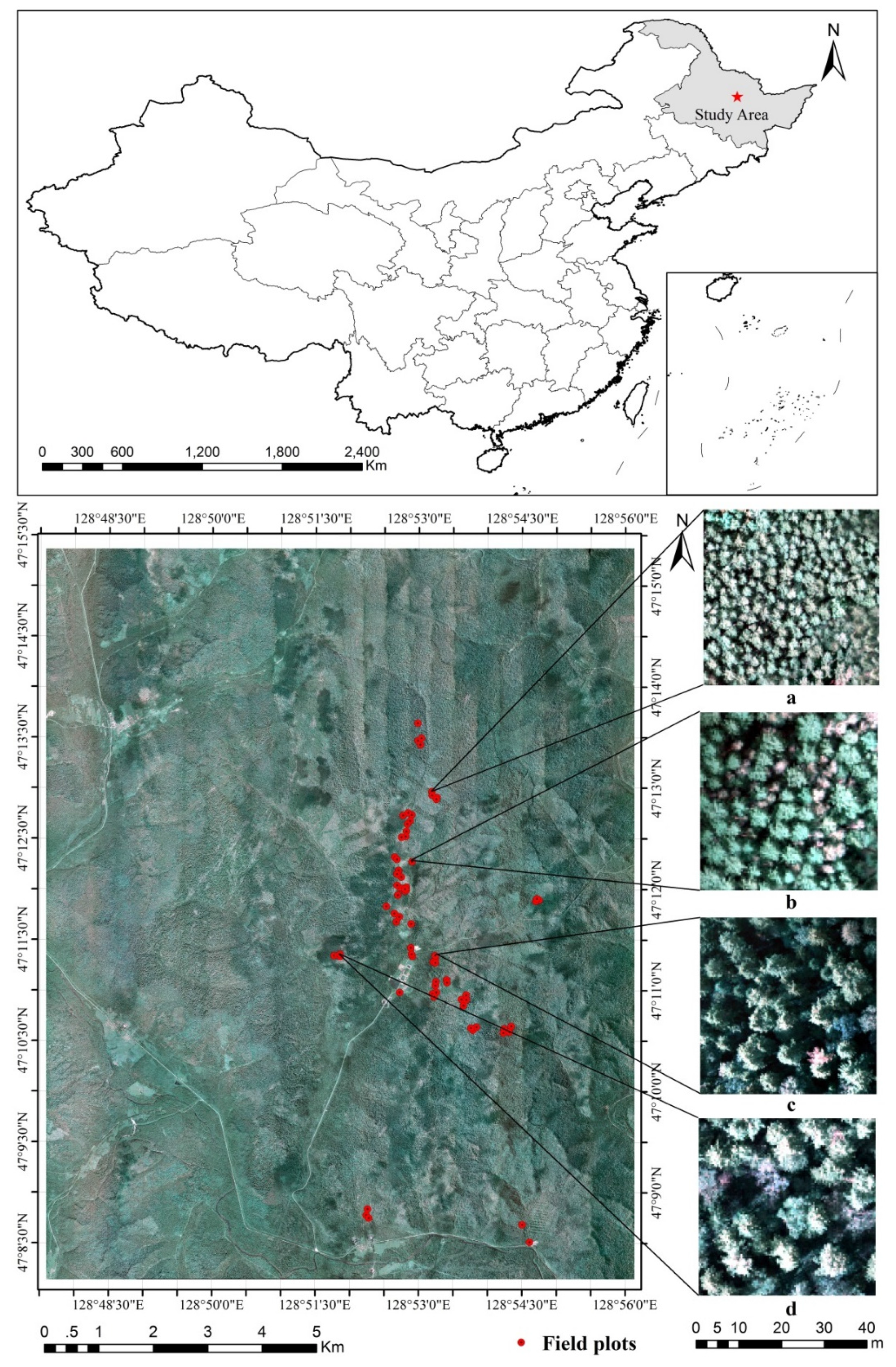
2.1. Study Area
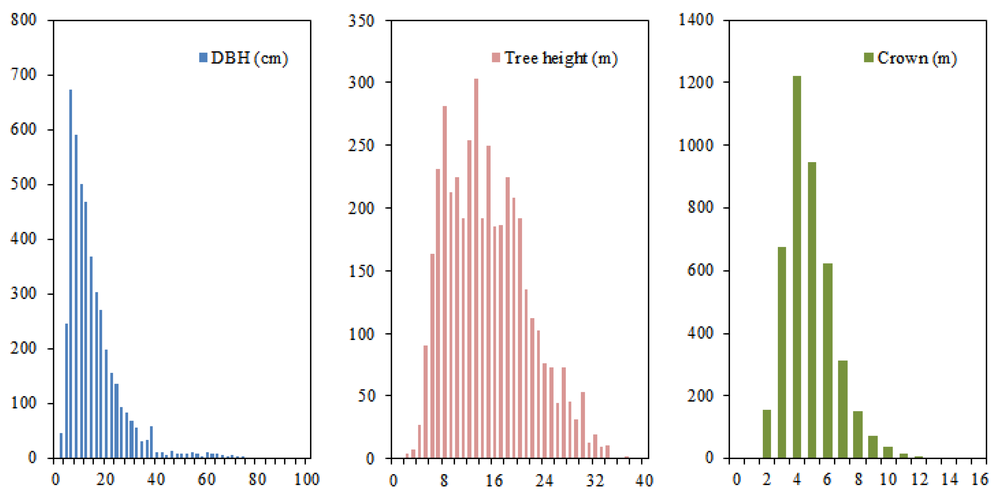
2.2. Field Data
2.3. Remote Sensing Data
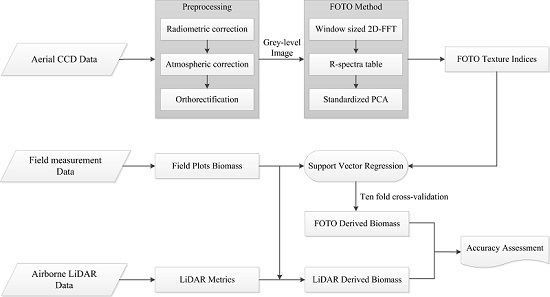
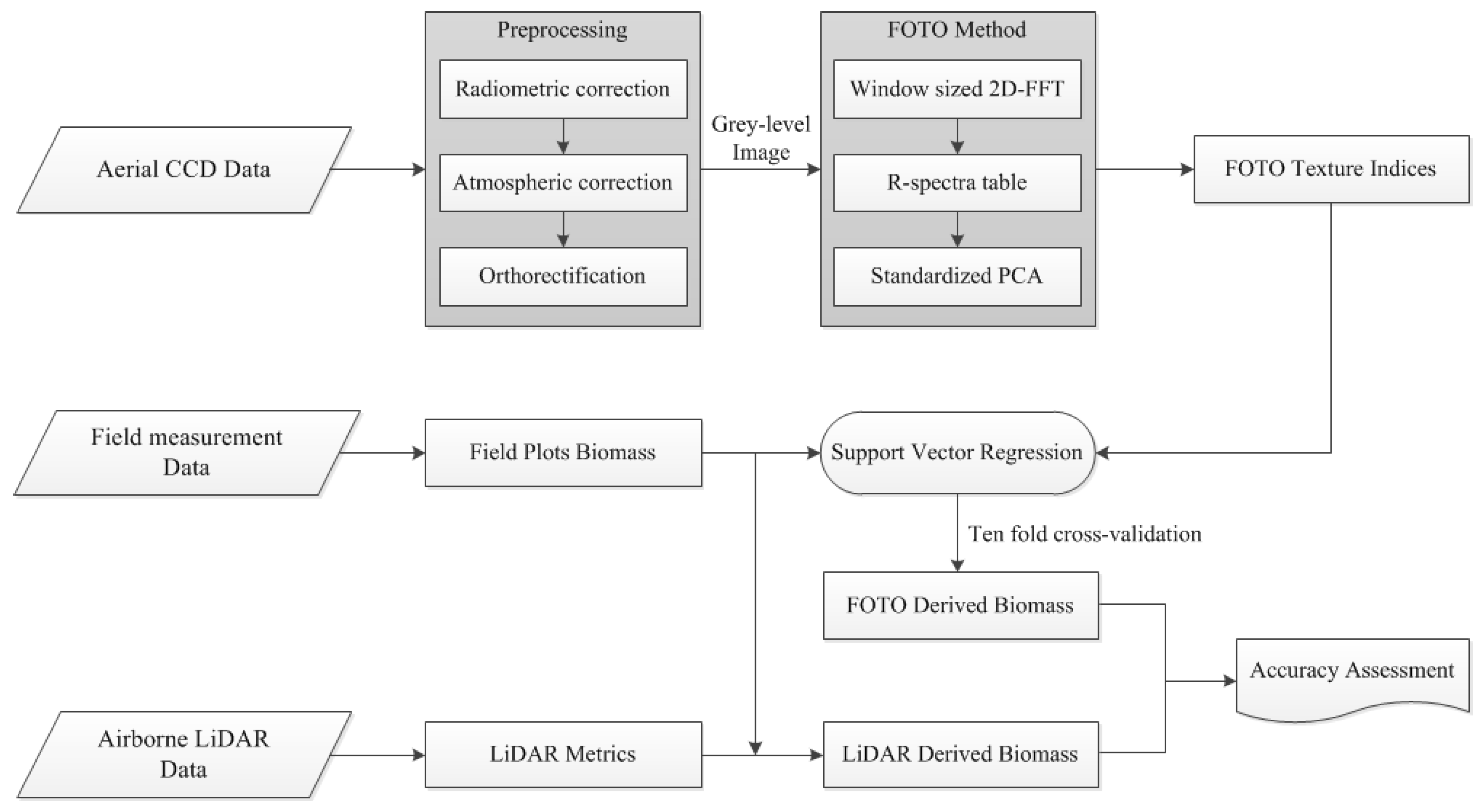
3. Methodology
3.1. FOTO Method
3.2. SVR and Validation
- The linear kernel:
- The polynomial kernel:
- The radial basis function (RBF) kernel:
- The sigmoid kernel:
4. Results and Discussion
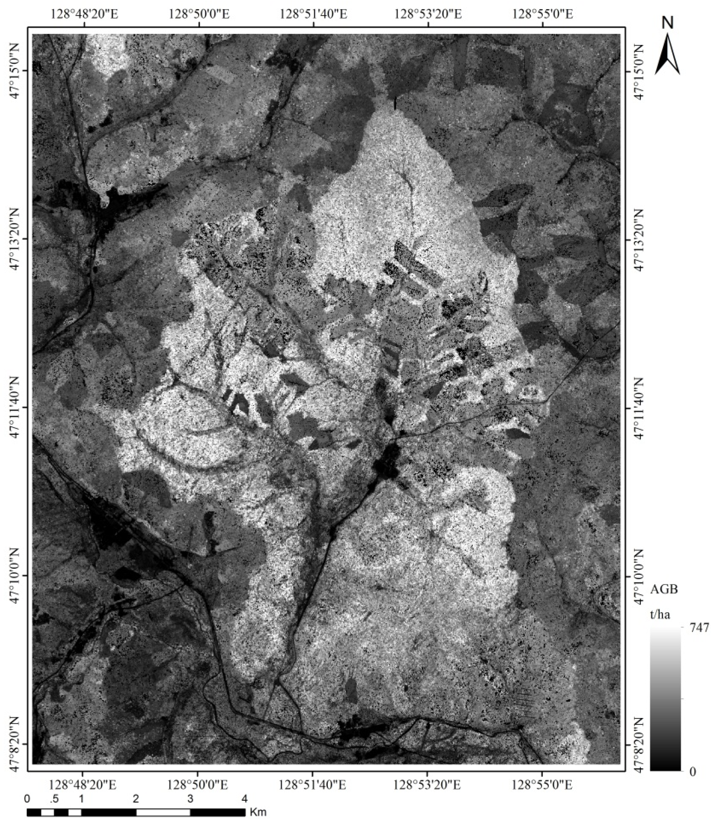
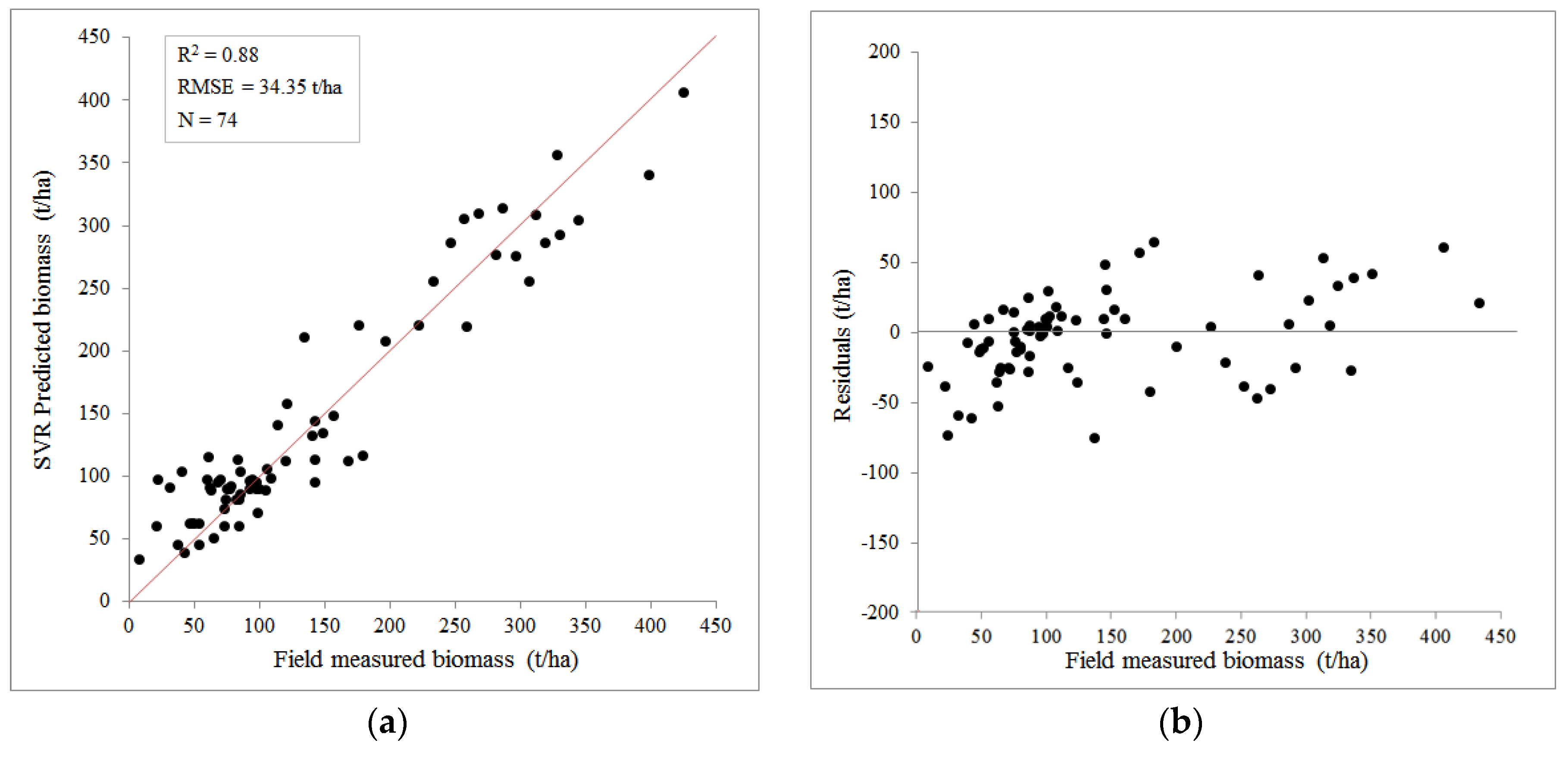
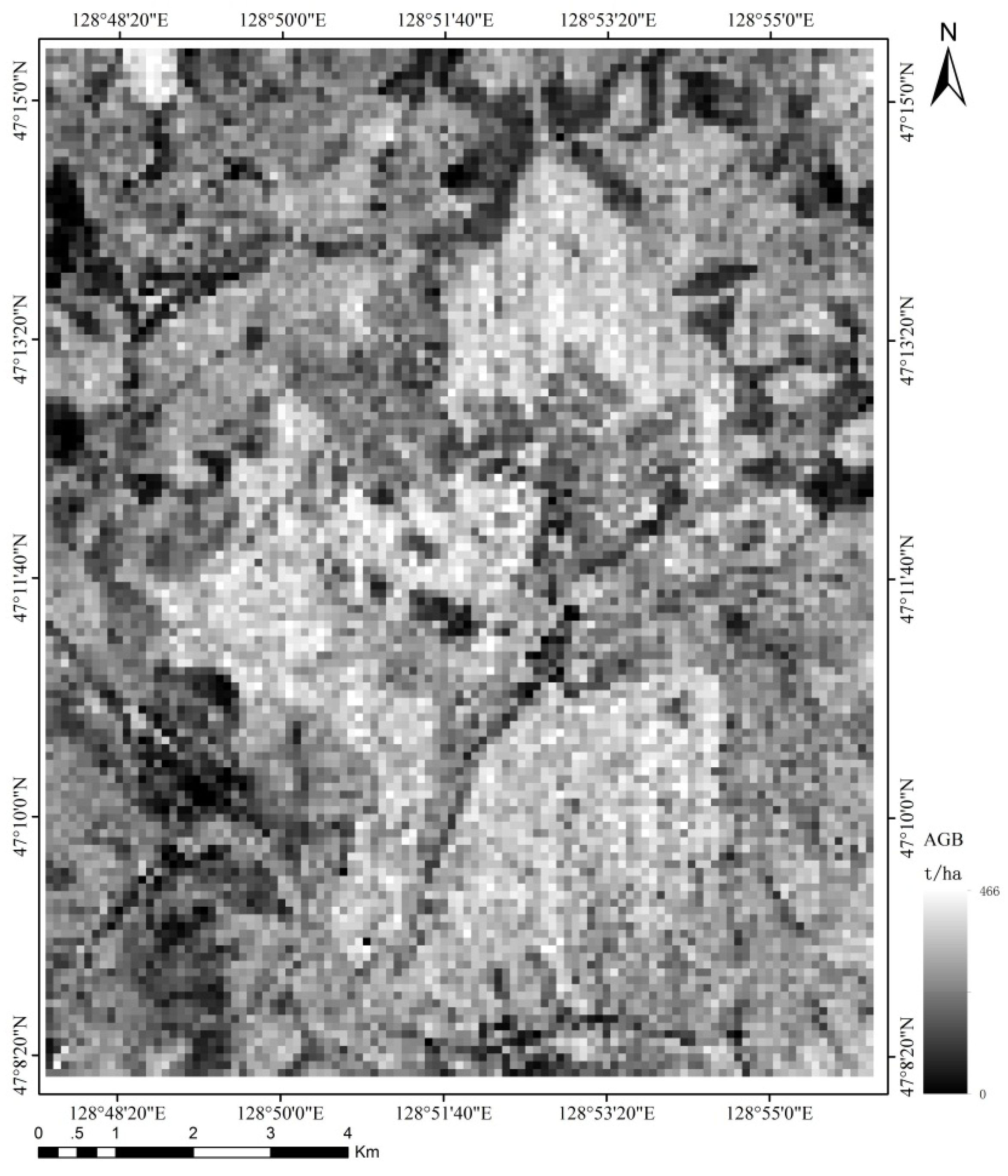
4.1. Forest AGB Estimation Using FOTO Texture Indices
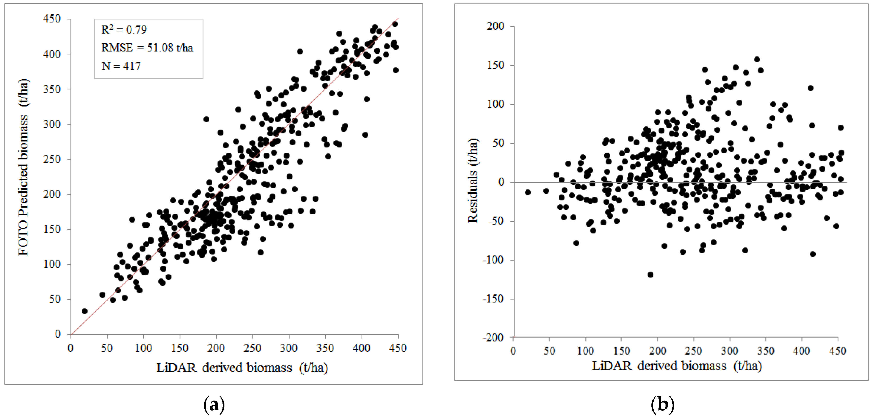
4.2. Intercomparison of FOTO Estimated Forest AGB Using a LiDAR-Derived AGB
4.3. Discussion
5. Conclusions
Acknowledgments
Author Contributions
Conflicts of Interest
References
- United Nations Framework Convention on Climate Change. Kyoto Protocol Reference Manual on Accounting of Emissions Assigned Amount. Available online: http://unfccc.int/ (accessed on 15 March 2015).
- Houghton, R.A. Aboveground forest biomass and the global carbon balance. Glob. Chang. Biol. 2005, 11, 945–958. [Google Scholar] [CrossRef]
- Brown, S.; Gaston, G. African Greenhouse Gas Emission Inventories and Mitigation Options: Forestry, Land-Use Change, and Agriculture; Springer: Berlin, Germany, 1995. [Google Scholar]
- Brown, S. Measuring carbon in forests: Current status and future challenges. Environ. Pollut. 2002, 116, 363–372. [Google Scholar] [CrossRef]
- Zheng, D.; Rademacher, J.; Chen, J.; Crow, T.; Bresee, M.; Lemoine, J.; Ryu, S. Estimating aboveground biomass using Landsat 7 ETM+ data across a managed landscape in northern Wisconsin, USA. Remote Sens. Environ. 2004, 93, 402–411. [Google Scholar] [CrossRef]
- Lu, D.S. The potential and challenge of remote sensing-based biomass estimation. Int. J. Remote Sens. 2007, 27, 1297–1328. [Google Scholar] [CrossRef]
- Lu, D.; Batistella, M. Exploring TM image texture and its relationships with biomass estimation in Rondônia, Brazilian Amazon. Acta Amazon. 2005, 35, 249–257. [Google Scholar] [CrossRef]
- Couteron, P.; Pelissier, R.; Nicolini, E.; Dominique, P. Predicting tropical forest stand structure parameters from Fourier transform of very high-resolution remotely sensed canopy images. J. Appl. Ecol. 2005, 42, 1121–1128. [Google Scholar] [CrossRef]
- Barbier, N.; Couteron, P.; Proisy, C.; Malhi, Y. The variation of apparent crown size and canopy heterogeneity across lowland Amazonian forests. Glob. Ecol. Biogeogr. 2010, 19, 72–84. [Google Scholar] [CrossRef]
- Maack, J.; Kattenborn, T.; Ewald, F.F.; Enssle, F.; Hernández, P.J.; Corvalán, V.P.; Koch, B. Modeling forest biomass using Very-High-Resolution data—Combining textural, spectral and photogrammetric predictors derived from spaceborne stereo images. Eur. J. Remote Sens. 2015, 48, 245–261. [Google Scholar] [CrossRef]
- Cedric, V.; Vepakomma, U.; Morel, J.; Bader, J.L.; Rajashekar, G.; Jha, C.S.; Ferêt, J.; Proisy, C.; Pélissier, R.; Dadhwal, V.K. Aboveground-Biomass Estimation of a Complex Tropical Forest in India Using Lidar. Remote Sens. 2015, 7, 10607–10625. [Google Scholar]
- Bastin, J.; Barbier, N.; Couteron, P.; Adams, B.; Shapiro, A.; Bogaert, J.; de Cannière, C. Aboveground biomass mapping of African forest mosaics using canopy texture analysis: Towards a regional approach. Ecol. Appl. 2014, 24, 1984–2001. [Google Scholar] [CrossRef]
- Singh, M.; Evans, D.; Friess, D.A.; Tan, B.S.; Chan, S.N. Mapping Above-Ground Biomass in a Tropical Forest in Cambodia Using Canopy Textures Derived from Google Earth. Remote Sens. 2015, 7, 5057–5076. [Google Scholar] [CrossRef]
- Proisy, C.; Couteron, P.; Fromard, F. Predicting and mapping mangrove biomass from canopy grain analysis using Fourier-based textural ordination of IKONOS images. Remote Sens. Environ. 2007, 109, 379–392. [Google Scholar] [CrossRef]
- Proisy, C.; Couteron, P.; Pelissier, R.; Engel, J. Monitoring canopy grain of tropical forest using Fourier-based textural ordination (FOTO) of very high resolution images. In Proceedings of the IEEE International Geoscience and Remote Sensing Symposium, IGARSS, Barcelona, Spain, 23–28 July 2007; pp. 4324–4326.
- Proisy, C.; Barbier, N.; Guéroult, M.; Pélissier, R.; Gastelluetchegorry, J.P.; Grau, E.; Couteron, P. Biomass prediction in tropical forests: The canopy grain approach. In Remote Sensing of Biomass: Principles and Applications; Intech: Rijeka, Croatia, 2011; pp. 1–18. [Google Scholar]
- Singh, M. Forest Structure and Biomass in a Mixed Forest-Oil Palm Landscape in Borneo. Master’s Thesis, University of Oxford, Oxford, UK, 2012. [Google Scholar]
- Singh, M.; Malhi, Y.; Bhagwat, S. Biomass estimation of mixed forest landscape using a Fourier transform texture-based approach on very high-resolution optical satellite imagery. Int. J. Remote Sens. 2014, 35, 3331–3349. [Google Scholar] [CrossRef]
- Ploton, P.; Pélissier, R.; Proisy, C.; Flavenot, T.; Barbier, N.; Rai, S.N.; Couteron, P. Assessing aboveground tropical forest biomass using Google Earth canopy images. Ecol. Appl. 2012, 22, 993–1003. [Google Scholar] [CrossRef] [PubMed]
- Lefsky, M.A.; Harding, D.; Cohen, W.B.; Parker, G.; Shugart, H.H. Surface Lidar remote sensing of basal area and biomass in deciduous forests of eastern Maryland, USA. Remote Sens. Environ. 1999, 67, 83–98. [Google Scholar] [CrossRef]
- Englhart, S.; Keuck, V.; Siegert, F. Modeling Aboveground Biomass in Tropical Forests Using Multi-Frequency SAR Data—A Comparison of Methods. IEEE J. Sel. Top. Appl. Earth Obs. Remote Sens. 2012, 5, 298–306. [Google Scholar] [CrossRef]
- Mora, B.; Wulder, M.A.; Hobart, G.W.; White, J.C.; Bater, C.W.; Gougeon, F.A.; Varhola, A.; Coops, N.C. Forest inventory stand height estimates from very high spatial resolution satellite imagery calibrated with LiDAR plots. Int. J. Remote Sens. 2013, 34, 4406–4424. [Google Scholar] [CrossRef]
- GOFC-GOLD. A Sourcebook of Methods and Procedures for Monitoring and Reporting Anthropogenic Greenhouse Gas Emissions and Removals Associated with Deforestation, Gains and Losses of Carbon Stocks in Forests Remaining Forests, and Forestation; GOFC-GOLD Report Version COP19-2; GOFC-GOLD Land Cover Project Office, Wageningen University: Wageningen, The Netherlands, 2013. [Google Scholar]
- Zhang, J.; Huang, S.; Hogg, E.H.; Lieffers, V.; Qin, Y.; He, F. Estimating spatial variation in alberta forest biomass from a combination of forest inventory and remote sensing data. Biogeosciences 2013, 10, 19005–19044. [Google Scholar] [CrossRef]
- García-Gutiérrez, J.; Martínez-Álvarez, F.; Troncoso, A.; Riquelme, J.C. A comparison of machine learning regression techniques for lidar-derived estimation of forest variables. Neurocomputing 2015, 167, 24–31. [Google Scholar] [CrossRef]
- Liu, L.; Pang, Y.; Fan, W.; Li, Z.; Zhang, D.; Li, M. Fused airborne LiDAR and hyperspectral data for tree species identification in a natural temperate forest. J. Remote Sens. 2013, 17, 679–695. [Google Scholar]
- Liu, J.; Liu, B.; Zhang, P. Scientific value and advantages of LiangShui nature conservation area. J. Wildl. 1993, 1, 4–5. (In Chinese) [Google Scholar]
- Pang, Y.; Li, Z.Y. Inversion of biomass components of the temperate forest using airborne Lidar technology in Xiaoxing’an Mountains, Northeastern of China. Chin. J. Plant Ecol. 2012, 36, 1095–1105. [Google Scholar] [CrossRef]
- Wang, C. Biomass allometric equations for 10 co-occurring tree species in Chinese temperate forests. For. Ecol. Manag. 2006, 222, 9–16. [Google Scholar] [CrossRef]
- Nilsson, M. Estimation of tree heights and stand volume using an airborne lidar system. Remote Sens. Environ. 1996, 56, 1–7. [Google Scholar] [CrossRef]
- Næsset, E.; Gobakken, T. Estimation of above- and below-ground biomass across regions of the boreal forest zone using airborne laser. Remote Sens. Environ. 2008, 112, 3079–3090. [Google Scholar] [CrossRef]
- Zhao, K.; Popescu, S.; Meng, X.; Pang, Y.; Agca, M. Characterizing forest canopy structure with lidar composite metrics and machine learning. Remote Sens. Environ. 2011, 115, 1978–1996. [Google Scholar] [CrossRef]
- Magnussen, S.; Boudewyn, P. Derivations of stand heights from airborne laser scanner data with canopy-based quantile estimators. Can. J. For. Res. 1998, 28, 1016–1031. [Google Scholar] [CrossRef]
- Robert, A. Simulation of the effect of topography and tree falls on stand dynamics and stand structure of tropical forests. Ecol. Model. 2003, 167, 287–303. [Google Scholar] [CrossRef]
- Harrison, J.M.; Lo, C.P. PC-based two-dimensional discrete Fourier transform programs for terrain analysis. Comput. Geosci. 1996, 22, 419–424. [Google Scholar] [CrossRef]
- Couteron, P. Quantifying change in patterned semi-arid vegetation by Fourier analysis of digitized aerial photographs. Int. J. Remote Sens. 2002, 23, 3407–3425. [Google Scholar] [CrossRef]
- Jachowski, N.R.A.; Michelle, S.Y.Q.; Daniel, A.F.; Decha, D.; Edward, L.W.; Alan, D.Z. Mangrove biomass estimation in Southwest Thailand using machine learning. Appl. Geogr. 2013, 45, 311–321. [Google Scholar] [CrossRef]
- Neumann, M.; Saatchi, S.S.; Ulander, L.M.H.; Fransson, J.E.S. Assessing Performance of L- and P-Band Polarimetric Interferometric SAR Data in Estimating Boreal Forest Above-Ground Biomass. IEEE Trans. Geosci. Remote Sens. 2012, 50, 714–726. [Google Scholar] [CrossRef]
- Zeng, Z.; Hsieh, W.W.; Shabbar, A.; Burrows, W.R. Seasonal prediction of winter extreme precipitation over Canada by support vector regression. Hydrol. Earth Syst. Sci. 2011, 15, 65–74. [Google Scholar] [CrossRef]
- Lin, X. A Simple Introduction to LIBSVM. Available online: http://www.csie.ntu.edu.tw/~cjlin/libsvm (accessed on 31 October 2015).
- Chang, C.C.; Lin, C.J. LIBSVM: A Library for Support Vector Machines. ACM Trans. Intell. Syst. Technol. 2006, 2, 389–396. [Google Scholar] [CrossRef]
- Smola, A.J.; Schölkopf, B. A tutorial on support vector regression. Stat. Comput. 2004, 14, 199–222. [Google Scholar] [CrossRef]
- Varma, S.; Simon, R. Bias in error estimation when using cross-validation for model selection. BMC Bioinform. 2006, 7. [Google Scholar] [CrossRef] [PubMed]
- Arlot, S.; Celisse, A. A survey of cross-validation procedures for model selection. Stat. Surv. 2009, 4, 40–79. [Google Scholar] [CrossRef]
- Eckert, S. Improved Forest Biomass and Carbon Estimations Using Texture Measures from WorldView-2 Satellite Data. Remote Sens. 2012, 4, 810–829. [Google Scholar] [CrossRef]
- Sarker, L.R.; Nichol, J.E. Improved forest biomass estimates using ALOS AVNIR-2 texture indices. Remote Sens. Environ. 2011, 115, 968–977. [Google Scholar] [CrossRef]


| Variables | Mean | Standard Deviation | Min | Median | Max | Skewness | Kurtosis |
|---|---|---|---|---|---|---|---|
| DBH (cm) | 16.33 | 11.33 | 2.10 | 13.31 | 98.70 | 2.47 | 8.47 |
| Tree height (m) | 14.72 | 6.48 | 1.80 | 14.04 | 38.90 | 0.55 | −0.21 |
| Crown diameter(m) | 4.36 | 1.64 | 0.15 | 4.12 | 15.80 | 1.04 | 1.97 |
| DigiCAM-H/22 | |||
| Sensor size | 5440 × 4080 | Pixel size | 9 μm |
| Sensor dimensions | 36.72 mm × 48.96 mm | Focal length | 50 mm |
| Riegl LMS-Q560 (Full Waveform Digitization) | |||
| Wavelength | 1550 nm | Point density | 2 points/m2 |
| Pulse firing rate | 100 kHz | Scan angle range | ±30° |
| Pulse length | 3.5 ns | Surface point accuracy (horizontal/vertical), excluding GPS errors | 0.1 m/0.03 m |
| Sampling interval | 1 ns | ||
© 2016 by the authors; licensee MDPI, Basel, Switzerland. This article is an open access article distributed under the terms and conditions of the Creative Commons by Attribution (CC-BY) license (http://creativecommons.org/licenses/by/4.0/).
Share and Cite
Meng, S.; Pang, Y.; Zhang, Z.; Jia, W.; Li, Z. Mapping Aboveground Biomass using Texture Indices from Aerial Photos in a Temperate Forest of Northeastern China. Remote Sens. 2016, 8, 230. https://doi.org/10.3390/rs8030230
Meng S, Pang Y, Zhang Z, Jia W, Li Z. Mapping Aboveground Biomass using Texture Indices from Aerial Photos in a Temperate Forest of Northeastern China. Remote Sensing. 2016; 8(3):230. https://doi.org/10.3390/rs8030230
Chicago/Turabian StyleMeng, Shili, Yong Pang, Zhongjun Zhang, Wen Jia, and Zengyuan Li. 2016. "Mapping Aboveground Biomass using Texture Indices from Aerial Photos in a Temperate Forest of Northeastern China" Remote Sensing 8, no. 3: 230. https://doi.org/10.3390/rs8030230
APA StyleMeng, S., Pang, Y., Zhang, Z., Jia, W., & Li, Z. (2016). Mapping Aboveground Biomass using Texture Indices from Aerial Photos in a Temperate Forest of Northeastern China. Remote Sensing, 8(3), 230. https://doi.org/10.3390/rs8030230