Fuzzy Classification for Shoreline Change Monitoring in a Part of the Northern Coastal Area of Java, Indonesia

Abstract

This study presents an unsupervised fuzzy c-means classification (FCM) to observe the shoreline positions. We combined crisp and fuzzy methods for change detection. We addressed two perspectives of uncertainty: (1) uncertainty that is inherent to shoreline positions as observed from remote sensing images due to its continuous variation over time; and (2) the uncertainty of the change results propagating from object extraction and implementation of shoreline change detection method. Unsupervised FCM achieved the highest kappa (κ) value when threshold (t) was set at 0.5. The highest κ values were 0.96 for the 1994 image. For images in 2013, 2014 and 2015, the κ values were 0.95. Further, images in 2003, 2002 and 2000 obtained 0.93, 0.90 and 0.86, respectively. Gradual and abrupt changes were observed, as well as a measure of change uncertainty for the observed objects at the pixel level. These could be associated with inundations from 1994 to 2015 at the northern coastal area of Java, Indonesia. The largest coastal inundations in terms of area occurred between 1994 and 2000, when 739 ha changed from non-water and shoreline to water and in 2003–2013 for 200 ha. Changes from water and shoreline to non-water occurred between 2000 and 2002 (186 ha) and in 2013–2014 (65 ha). Urban development in flood-prone areas resulted in an increase of flood hazards including inundation and erosion leading to the changes of shoreline position. The proposed methods provided an effective way to present shoreline as a line and as a margin with fuzzy boundary and its associated change uncertainty. Shoreline mapping and monitoring is crucial to understand the spatial distribution of coastal inundation including its trend.

1. Introduction

Shoreline location and its change in position are critical for understanding coastal structures [1], safe navigation [2,3], sustainable coastal resource management [4], and for flood protection and other risk management [5,6]. Furthermore, shoreline mapping and monitoring can help to understand the spatial distribution of coastal inundation including its trend over time.

In the literature, shoreline is defined as an intersection of coastal land and water surface indicating water edge movements as the tides rise and fall [7,8,9]. Even though shoreline position can be defined as the waterline at various stages of the tides, e.g., high tide, mid tide, and low tide, the shoreline is largely associated with the sea level [10]. Ideally, the shoreline is the physical interface of land and water with its position changing through time (Doland et al. (1980) in Boak and Turner [8]). Its change results from long-term, cyclic and random variation. Long-term variation includes variation due to sediment storing or due to the relative sea level rise. Cyclic variation is a combination of seasonality and tide, whereas waves, storms and floods cause random variation of a local character.

To properly extract trends from shoreline positions has been a subject of considerable interest. Due to the dynamic nature of the shoreline, shoreline indicators were used as a proxy to represent the “true” shoreline position. Boak and Turner [8] and Gens [11] distinguished: (1) a feature that can be distinguished in a coastal imagery; for example, the high water line (HWL) [12,13]; (2) the intersection of a tidal datum with a coastal profile, such as the mean high water (MHW); and (3) proxy shoreline features extracted from digital images at the coast, e.g., water and non-water pixels following a binary classification [14,15].

Ground surveys and photogrammetry have been used widely to detect shoreline position [3]. Both methods are relatively expensive and time consuming, hence data derived from remote sensing platforms are widely used nowadays [8]. Wang [16] and Dewan and Yamaguchi [17] applied the optimal threshold values to separate water and non-water by giving different cut-off values for each dataset of Landsat TM images. Senthilnatha, et al. [18] used a genetic algorithm and particle swarm optimization to distinguish the water from the non-water region, based on time-series analysis of images. Martinis, et al. [19] applied spectral indices EVI (Enhanced Vegetation Index), LSWI (Land Surface Water Index) and DVEL (Difference Value between EVI and LSWI) to detect water on MODIS data. Ouma and Tateishi [20] and Ghosh, et al. [15] generated a water index to produce a binary class of water and non-water, then manually digitized the result to produce a shoreline map. Other methods such as post-classification comparison [21], binary slicing [22], masking operation and visual interpretation [23,24] have been implemented to derive shoreline change maps.

Many studies on shoreline mapping used hard classifications, whereas few studies exist for fuzzy classification of shorelines [25,26]. A hard classification assigns a single label to a pixel, thus allocating each pixel to the class to which it has its highest membership. This could be misleading, because a shoreline is by definition the physical interface of coastal land and water surface with its position changing through time. There is a transition zone between water and land, and hence the boundary is imprecise. In addition, manual digitizing methods are time consuming, costly and labour intensive as they are associated with the large amount of image data required for shoreline mapping and monitoring. Because of these limitations, this study explores fuzzy classification in deriving proxy shoreline features from digital images. Moreover, to map the dynamic shoreline positions and to extract their changes requires the handling of uncertainty. Most studies regarding shoreline change detection explored uncertainty modelling with a focus on aerial imagery [27,28] and a statistical uncertainty analysis [29,30]. Our study focuses on: (1) inherent uncertainty due to continuous variation of a shoreline over time; and (2) uncertainty as it propagates from extraction and implementation of the shoreline change detection method.

To deal with these uncertainties, fuzzy c-means (FCM) classification developed by Bezdek, et al. [31] was applied. Unsupervised FCM for two classes (water and non-water) is expected to support a rapid mapping of shoreline changes and give an accurate shoreline position by allowing multiple memberships for a pixel. The current study extends that approach by including tide condition. Thus, a change detection method was implemented to distinguish abrupt and gradual changes at the object level and provide the change uncertainty at the pixel level.

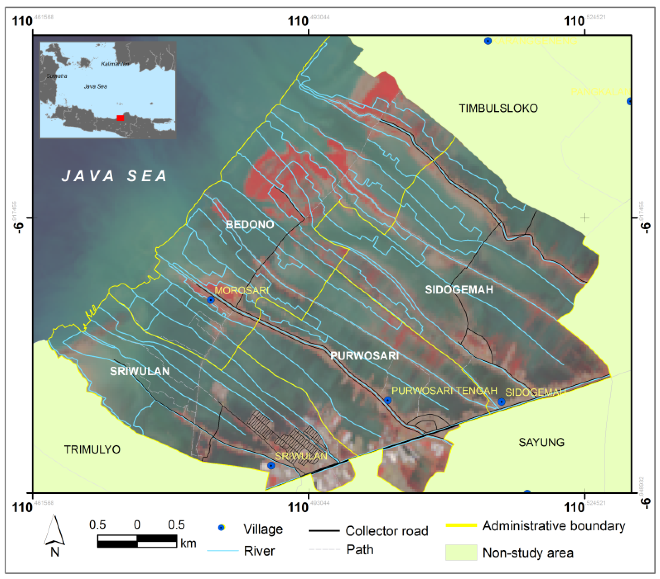
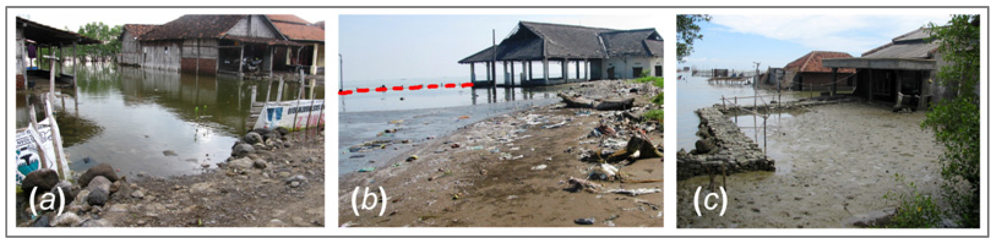
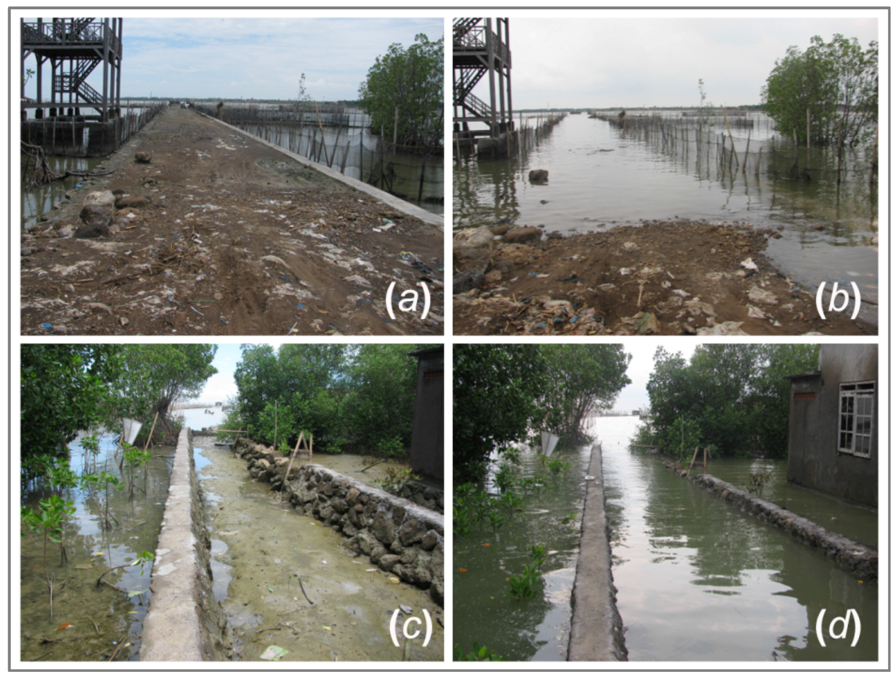
The objective of this study was to develop a fuzzy method that is useful for detecting shoreline changes from multi-temporal images by taking the gradual transition between water and land and the tides into account. The method, based on fuzzy classification and change uncertainty, will be described by means of possibility and necessity measures. The method is applied to an area in Java, where the northern coastal area of Sayung sub-district experienced a severe change of shoreline position.

2. Methodology

2.1. Study Area

This study was carried out in a part of the Sayung sub-district in the northern coastal area of Central Java Province extending 5 km from east to west (Figure 1). The area has faced a severe impact of coastal inundation which has led to a significant change of shoreline position over the past two decades (Figure 2). The average tidal range in this location is 60 cm with the highest tidal ranges occurring in December and June during the rainy and dry seasons, and the lowest tidal ranges in March and September during the transitional seasons.

The area is characterized by a flat topography ranging between 0 and 5 m above mean sea level (AMSL). As a lowland coastal area, it is dominated by alluvial clay and sand sedimentation with more than 10 rivers running across the area and carrying sediments from the upstream areas [32,33]. The poor drainage system leads to a regular occurrence of floods during the rainy season. Meanwhile, the areas adjacent to the sea are prone to the impact of tidal flood which occurs daily in line with the tides [34,35]. In this study area, four villages are located amidst extensive fishponds and rice fields. Settlements are found along the riverbanks or adjacent to the shorelines. Since the 1990s, the productive rice fields became inundated and were converted into fishponds, or merely abandoned as swamp areas [32].

An extensive change of shoreline has been occurring for more than 20 years (Figure 3) caused by natural processes, e.g., coastal inundation, erosion, and sedimentation and by the development of man-made structures, e.g., beach reclamation and extended seaport. Moreover, the coastal inundation accelerating these changes has increased recently in terms of frequency and duration as a result of many factors. These include at the short term: extreme winds, heavy rains, and at the long term: land subsidence, sea level rise, mangrove conversion, groundwater extraction, construction load, and the increase of impervious surface [34,36,37,38]. Many efforts have been made by the Demak local government to overcome the erosion of 80 km² of land [39] and curb the coastal inundation which leads to the dramatic changes of the shoreline. Efforts include embankment, elevated road, breakwater, and mangrove planting.

2.2. Satellite Images and Data Pre-Processing

Landsat images from three different sensors were used to monitor the shoreline change between 1994 and 2015. Landsat has a 16-day revisit time, and passes Indonesia at approximately 02.00–03.00 GMT. Six spectral bands of Landsat TM and ETM and seven spectral bands of Landsat OLI/TIRS were used. Spectral bands of Landsat TM and ETM applied in this research cover the blue (0.45–0.515 µm), green (0.525–0.605 µm), red (0.63–0.69 µm), near infrared (0.75–0.90 µm), shortwave infrared 1 (1.55–1.75 µm) and shortwave infrared 2 (2.09–2.35 µm) parts of the electromagnetic spectrum. In addition, the spectral bands of Landsat OLI/TIRS included in FCM consisted of coastal and aerosol (0.43–0.45 µm), blue (0.45–0.51 µm), green (0.53–0.59 µm), red (0.64–0.67 µm), near infrared (0.85–0.88 µm), shortwave infrared 1 (1.57–1.65 µm) and shortwave infrared 2 (2.11–2.29 µm).

Table 1. Landsat images from three different sensors (Thematic Mapper, Enhanced Thematic Mapper, Operational Land Imager/Thermal Infrared Sensor) supplemented by astronomical tide level, and reference data. All images were captured in the low tides.

Acquisition Date	Acquisition Time (GMT)	Sensor	Astronomical Tide Level (m)	Reference Data
11 November 1994	02:02	TM	−0.321	Topographic map, 1994 (published on 2000)
5 December 2000	02:41	ETM	−0.215	QuickBird image acquired on 3 May 2003
11 December 2002	02:36	ETM	−0.364	QuickBird image acquired on 3 May 2003
2 April 2003	02:36	ETM	−0.118	QuickBird image acquired on 3 May 2003
27 August 2013	02:50	OLI/TIRS	−0.054	Pleiades image acquired on 27 February 2013
8 April 2014	02:48	OLI/TIRS	−0.025	Image via Google Earth acquired on 1 July 2014
26 March 2015	02:47	OLI/TIRS	−0.109	Field measurement (2015)

shows the images used in this study supplemented by tidal data. Tidal data in accordance with the time of acquisition of the images was collected from the Indonesia Geospatial Information Agency.

Pre-processing consisted of histogram minimum adjustment to reduce the effect of atmospheric path radiance [40,41], followed by geo-referencing using >100 ground control points (GCP) that were carefully selected on both Landsat and ortho-rectified WorldView-2 images from road intersections, building corners, wall boundaries, river and other prominent features, and re-sampling to a 30 m pixel size using the nearest neighbour resampling method and third order polynomial transform algorithm. The root mean square error (RMSE) was less than 0.1 pixels.

2.3. Fuzzy C-Means (FCM) Classification and Parameter Estimation

The FCM iterative clustering method developed by Bezdek, et al. [31] was performed on the images to discriminate the land and water classes. FCM separates data clusters with fuzzy means and fuzzy boundaries allowing for partial membership. Let $Y=\left\{y_1,y_2,\dots ,y_N\right\}$ be a sample of the N pixels on an image, with $y_kϵR^n$ where n is the number of bands in an image, i.e., n = 6 or n = 7 for Landsat images used here. Let c denote the number of subsets (clusters or partitions) with $2\le c\le N$. In this research, we have c = 2 for the classes water and non-water, respectively, since we considered the boundary between these two classes as the shoreline position. FCM minimizes the following objective function $J_m$ [31]:

$$J_m={\displaystyle \sum }_{k=1}^N{\displaystyle \sum }_{i=1}^c{\left({\mu }_{\text{ik}}\right)}^m{\left|\right|y_k-v_i\left|\right|}^2,1\le m\le \infty$$

(1)

where ${\mu }_{ik}$ is the membership value of $k^{th}$ pixel to class i, m is the fuzzy weight controlling the level of fuzziness, and $v_i=\left(v_{i1},v_{i2},.\mathrm{..},v_{in}\right)$ is the mean vector for class i. The membership value ${\mu }_{ik}$ for class i and pixel k satisfies the following constraints:

$$0\le {\mu }_{ik}\le 1i\in \left\{1,\dots .,c\right\},k\in \left\{1,\dots ,N\right\}$$

(2)

$${\displaystyle \sum }_{k=1}^N{\mu }_{ik}>0,i\in \left\{1,\dots ,c\right\}$$

(3)

$${\displaystyle \sum }_{i=1}^c{\mu }_{ik}=1,k\in \left\{1,\dots .,N\right\}$$

(4)

There should be at least one class for which the membership value ${\mu }_{ik}$ of the $k^{th}$ pixel larger than 0. Meanwhile, the sum of all memberships ${\mu }_{ik}$ in a pixel should be equal to 1. The membership values of the classification corresponding to the pixel value Y follow the trapezoidal membership function in Figure 4 and Equation (5):

$$\mu \left(y,a,b,c,d\right)=\{\begin{array}{c}0,y<a,\\ \frac{y-a}{b-a},a\le y\le b\\ 1,b<y<c\\ \frac{d-y}{d-c},c\le y\le d\\ 0,y>b\end{array}$$

(5)

If m equals 1, clusters that minimize the objective function are hard clusters and FCM is a hard classifier. An increase of m tends to an increase in fuzziness. Bezdek, et al. [31] further explained that no evidence distinguishes an optimal m, but for most data, $1.5\le m\le 3.0$ give good results. In addition, Foody [42] stated that in most studies, m = 2.0 produces an accurate fuzzy classification. In this work, the values m = 1.5, 1.6, 1.7, 1.8, 1.9, 2.0, 2.5, and 3.0 were used to test the influence of m on the classification results.

FCM was finalized by labelling one of the two membership images resulting from each (unsupervised) FCM as the water membership image. To do so, we used the combination of near infrared (NIR) and shortwave infrared (SWIR) of Landsat bands. Infrared bands exhibit a strong contrast between water and land features, because water absorbs these wavelengths while they are reflected by land [43]. In the visible part of the spectrum, the differences between land and water are less outspoken, especially if the water contains some sediment. Therefore, the water label was given to the class which has the lowest value of the sum of the cluster means in the infrared bands, defined as:

$$FC{M}_{water}=MIN\left[{\left(v{i}_{c1}\right)}_{IR},{\left(v{i}_{c2}\right)}_{IR}\right]$$

(6)

where $v{i}_{c1}$ is the sum of mean vector for the first class in the infrared bands IR, and $v{i}_{c2}$ is the sum of mean vector for the second class in the infrared bands IR.

Table 2. Mean vector of two subsets in the infrared bands of 2015 Landsat image. The labelling of c1 or c2 as water was determined by assessing the sum of the mean vector cluster.

Subset	Mean Vector of the Cluste		r in the Infrared Bands ($vi)$	Total (Band5 + Band6 + Band7)
	Band5	Band6	Band7
c1	2085.711	925.3242	591.7152	3602.75
c2	8824.05	7427.402	5240.535	21,491.99

shows an example of cluster means of each subset in the infrared bands. The labelling of c1 or c2 as water was decided by using Equation (6). In this example, the water label was given to c1 as it has the lowest value of the sum of the cluster means in the infrared bands.

2.4. Deriving Water Class Images

Water membership images, resulting from the FCM classification, show the membership of pixels to the water class. Thresholding was applied to transform the water membership image into several hard classifications. The class $C$ in water class images was defined as:

$$C=\{\begin{array}{c}1if{\mu }_{ik}\ge t\\ 0otherwise\end{array}$$

(7)

where 1 is water class, 0 is non-water class, and t is threshold value. The possible ranges of the threshold values are between 0 and 1. In this study, we set the value of t between 0.1 and 0.9 to observe the influence of t on the results of classification. The results of thresholding were binary images called water class images.

2.5. Accuracy Assessment

Reference data are described in Table 1. For the 2015 image, reference data were derived from fieldwork conducted at the end of March 2015. In this case, 150 points from fieldwork data were selected based on the same tide condition. Furthermore, an image made available via Google Earth 2014 captured during the high tide, a 2013 Pleiades image during low tide, and a 2003 QuickBird image captured during the rising tide were interpreted visually to generate 150 reference points. Further, because of limited availability of high-resolution images and maps, the 2003 QuickBird image was used as well for accuracy assessment of images in 2000 and 2002. Finally, the topographic map published in 2000 and generated from aerial photographs of 1994 was manually digitized on-screen to produce water and non-water classes. For this map, 150 points were randomly selected, and were used as reference data against the classification result of the 1994 image. To evaluate how well the remotely sensed classifications agree with the reference data, error matrices were generated. A kappa (κ) coefficient was computed for each error matrix [43].

2.6. Shoreline Generation

Two methods were followed to identify the shoreline. The first method determined shoreline as a single line, as has been widely considered in the previous studies, whereas the second method assumed shoreline as a margin, which reflects the possible locations of shoreline influenced by the membership to the water class in a pixel.

2.6.1. Shoreline as a Single Line

First, the shoreline was derived by generating water class image and set t = 0.5. Two sub-areas were identified, namely water and non-water. Shoreline was located at the boundary of the two sub-areas and obtained by converting the water class image to line features in GIS. For this research, a sub-area was defined as a set of contiguous cells with the same value.

2.6.2. Shoreline as a Margin

Secondly, we considered the shoreline as an area (margin). The shoreline margin was generated by creating a crisp sub-area determined by t = 0.3 and t = 0.7 as the lower and upper thresholds obtained in the parameter estimation. Afterwards, each water class image was converted into polygon feature in GIS. Thus, three sub-areas were identified, namely water if ${\mathsf{\mu }}_{ik}\ge 0.7$, non-water if ${\mathsf{\mu }}_{ik}<0.3$ and shoreline margin if $0.3\le {\mathsf{\mu }}_{ik}<0.7$. Over time, the changes of shoreline position are due to the exchanges between the shoreline margin and water or non-water sub-area.

2.7. Uncertainty Estimation

Considering the imprecise position of the shoreline in remote sensing images and the uncertainty propagated through the change detection method, shoreline margin, water and non-water sub-areas were associated with values reflecting the uncertainty of pixels belonging to any of these classes. Water membership values were used for this purpose. The certainty of pixel k to belong to any class was assessed using possibility and necessity measures [44,45,46,47]. If C is a subset of a universe of discourse U and $x\in C$, then ${\mathsf{\pi }}_x\left(u\right)$ is the degree of possibility that x takes value u. The value of ${\mathsf{\pi }}_x\left(u\right)$ is evaluated by the degree of membership ${\mathsf{\mu }}_C\left(u\right)$. This can be written as:

$${\pi }_x\left(u\right)={\mathsf{\mu }}_C\left(u\right),\forall u\in U$$

(8)

The value of $x\in C$ is then estimated by assessing possibility measure:

$${\Pi }_C=\underset{u\in C}{\sup }{\pi }_x\left(u\right)$$

(9)

The possibility measure ${\Pi }_C$ corresponds to the element of C that has the highest possibility degree according to ${\mathsf{\pi }}_x$. Further, to inform that the event will be realized, the certainty of C is defined as the impossibility of the complement:

$$N_C=1-{\Pi }_{\overline{C}}$$

(10)

$$N_{\overline{C}}=1-{\Pi }_C$$

(11)

The N pixels in Y are therefore indicated as C if ${\Pi }_C>{\Pi }_{\overline{C}}\text{\hspace{0.17em}and\hspace{0.17em}}{N}_C>N_{\overline{C}}$. Further, the uncertainty of C is defined as:

$$U_C=1-N_C$$

(12)

2.8. Shoreline Change Detection

To detect the changes in the positions of the shoreline, shoreline margin, water and non-water areas, results for two dates $T_1$ and $T_2$ had to be superimposed in GIS. In order to have a detailed “from-to” change trajectory information, the post-classification comparison approach was used [48]. Topological relation between two sub-areas can be characterized by considering the nine-intersection model of interiors and exteriors [49,50]. Based on this method, a sub-area identified at time $T_1$ is denoted as $R_{T1}$, with the boundary $B(R_{T1})$, interior $I\left(R_{T1}\right)$, and exterior $E\left(R_{T1}\right)$. It intersects with another sub-area identified in time $T_2$ and denoted as $R_{T2}$, with the boundary $B(R_{T2})$, interior $I\left(R_{T2}\right)$, and exterior $E\left(R_{T2}\right)$. These intersections define the nine-intersection matrix as:

$$M=\left(\begin{array}{ccc}B(R_{T1}){{\displaystyle \cap }}^{\text{}}B(R_{T2})& B(R_{T1}){{\displaystyle \cap }}^{\text{}}I(R_{T2})& B(R_{T1}){{\displaystyle \cap }}^{\text{}}E(R_{T2})\\ I(R_{T1}){{\displaystyle \cap }}^{\text{}}B(R_{T2})& I(R_{T1}){{\displaystyle \cap }}^{\text{}}I(R_{T2})& I(R_{T1}){{\displaystyle \cap }}^{\text{}}E(R_{T2})\\ E(R_{T1}){{\displaystyle \cap }}^{\text{}}B(R_{T2})& E(R_{T1}){{\displaystyle \cap }}^{\text{}}I(R_{T2})& E(R_{T1}){{\displaystyle \cap }}^{\text{}}E(R_{T2})\end{array}\right)$$

(13)

with intersections being either empty $(\varnothing )$ or non-empty $\left(\neg \varnothing \right)$. Figure 5 shows eight topological relationships of two sub-areas for each intersection value in the matrix M including disjoint, meet, overlap, contains, inside, covers, covered by, and equal [49].

Following the aforementioned methods in the shoreline generation, the changes of shoreline and its change uncertainty can be presented as follows:

2.8.1. Shoreline as a Single Line

In the first method, the changes of this single shoreline may have occurred as a consequence of changes between water and non-water sub-areas. We determined the changes of these sub-areas at times $T_1$ and $T_2$ and analyzed the uncertainty of the changes at pixel level. Water class images from two dates $T_1$ and $T_2$ were superimposed, and abrupt and gradual changes were identified. An abrupt change is defined when a sub-area emerges at $T_2$ without a corresponding sub-area at $T_1$. Also, a sub-area present at $T_1$ without a corresponding sub-area at $T_2$ indicates an abrupt change. A gradual change specifies an increase or decrease of sub-areas that were both present at $T_1$ and $T_2$. The process occurs in small stages over a period rather than suddenly. The overlay analysis between images at different epochs permitted the identification of changes categorized as: water to non-water, and non-water to water. Considering the topological relationship as given in Figure 5, disjoint and meet were found where a sub-area emerges or disappears. Meanwhile, any of the other six relationships account for gradual changes.

2.8.2. Shoreline as a Margin

The second method measured the changes of the shoreline margin at different epochs. Change uncertainty was presented at the pixel level. Water class images from times $T_1$ and $T_2$ were superimposed in a GIS. We distinguished again abrupt and gradual change. In this method, the overlay analysis between water class images at different epochs, however, permitted more changes to be identified categorized as: (1) shoreline to non-water; (2) water to shoreline; (3) water to non-water; (4) non-water to shoreline; (5) shoreline to water; and (6) non-water to water. The changes of a sub-area where sedimentation has taken place resulted in changes of shoreline to non-water, water to shoreline, and water to non-water. These types of changes were considered positive changes to non-water sub-area (+). Coastal inundation led to the changes of non-water to shoreline, shoreline to water, and non-water to water. These types of changes were considered negative changes to non-water sub-area (−). These changes were identified either as abrupt or gradual changes, using the same criteria on corresponding objects as in the previous section.

2.9. Change Uncertainty and Change Area Estimation

Shoreline changes and the related sub-areas were associated with change uncertainty values. Change uncertainty was derived based upon the uncertainty of pixels belonging to the specified sub-areas in $T_1$ and $T_2$ [51]:

$$C{U}_{T_1,T_2}=MIN\left[U_c\left(R_{T1}\right),U_c\left(R_{T2}\right)\right]$$

(14)

where $U_c\left(R_{T1}\right)$ is the uncertainty of pixel k belonging to sub-area $R_{T1}$ at $T_1$, and $U_c\left(R_{T2}\right)$ is the uncertainty of pixel k belonging to sub-area $R_{T2}$ at $T_2.$ Based upon the results of the change uncertainty estimation, the changed area of a specific change category, e.g., water to non-water, or shoreline to water was defined as:

$$A\left(Ch\right)=P_k\left(Ch\right)\times A\left(k\right)$$

(15)

where $P_k\left(Ch\right)$ is number of pixels belonging to the area of a specific change category, $A\left(k\right)$ is area of pixel k equal to $30\times 30$ (m²).

2.9.1. Change Area of Shoreline as a Single Line

Figure 6 illustrates the procedure to estimate the net change between $T_1$ and $T_2$ defined as:

$$C{H}_{T_1,T_2}=P_k\left(C{h}_A\right)-P_k\left(C{h}_B\right)$$

(16)

where A and B represent the area described in Figure 6, and $P_k\left(C{h}_A\right)$ and $P_k\left(C{h}_B\right)$ are the number of pixels belonging to the change area A and B, respectively.

The negative sign (−) shows that the change in B categorized as the change from non-water to water has produced a negative change to the non-water area. Meanwhile, the positive sign (+) represents the change in A categorized as the change from water to non-water which has caused a positive change to the non-water area.

2.9.2. Change Area of the Shoreline as a Margin

Figure 7 illustrates the procedure to estimate the total changed area in the second approach. The net changed area was determined as:

$$C{H}_{T_1,T_2}=P_k\left(C{h}_A\right)+P_k\left(C{h}_B\right)+P_k\left(C{h}_C\right)-P_k\left(C{h}_D\right)-P_k\left(C{h}_E\right)-P_k\left(C{h}_F\right)$$

(17)

where A, B, C, D, E, and F represent the area described in Figure 7, and $P_k\left(C{h}_A\right),P_k\left(C{h}_B\right),P_k\left(C{h}_C\right),P_k\left(C{h}_D\right),P_k\left(C{h}_E\right)$ and $P_k\left(C{h}_F\right)$ are the number of pixels belonging to changed areas A,…,F, respectively.

The positive sign (+) indicates that the changes in A, B and C have caused a positive change to the shoreline margin and non-water areas. On the other hand, the negative sign (−) shows that the changes in D, E, and F have induced a negative change to the shoreline margin and non-water areas.

3. Results

3.1. Parameter Estimation

Figure 8 provides the results of the κ value for parameter estimation of the fuzzy weight (m) conducted on seven images with t values ranging from 0.1 to 0.9. From the results, we found that the highest κ value was obtained for t = 0.5. The variation in fuzzy weight had little influence on the classification results when the t was set at 0.5. High κ values were obtained for t values between 0.3 and 0.7, and m values between 1.5 and 3.0. Best results in terms of κ values were obtained for m = 1.7. Furthermore, we selected t values of 0.3, 0.5, and 0.7 as the lower, the middle, and the upper t respectively, as the optimal t values to handle the uncertainty of the water class.

3.2. FCM Classification, Thresholding and Accuracy Assessment

Table 3. The accuracy of unsupervised FCM classification applied at selected parameter m = 1.7 and t = 0.3, 0.5 and 0.7. For all images, t = 0.5 obtained the highest kappa (κ) values, t = 0.7 produced slightly lower κ values, and t = 0.3 resulted in the lowest κ values.

Classified Images	κ Coefficient for Selected t Values
	0.3	0.5	0.7
1994	0.95	0.96	0.96
2000	0.81	0.86	0.81
2002	0.85	0.90	0.85
2003	0.87	0.93	0.89
2013	0.86	0.95	0.90
2014	0.83	0.95	0.90
2015	0.90	0.95	0.92

presents the κ values of FCM implemented with m = 1.7 and t = 0.3, 0.5, and 0.7, respectively. Unsupervised FCM achieved the highest κ value when t = 0.5. The value of κ was slightly lower for t = 0.7, and the lowest κ for t = 0.3. When comparing images, the lower κ values were observed for the images of 2000 and 2002. Such lower accuracies could be due to the use of QuickBird image 2003 as reference data. The acquisition time of the 2003 QuickBird and Landsat images (2000 and 2002) differs more than a year. Therefore, changes of some locations due to village development, seasonal and tide condition could affect the selection of an appropriate sample point.

Figure 9 shows FCM results for m = 1.7 presenting the membership to the water class ranging from 0 to 1, together with classified images for t = 0.5. Areas with a high membership to the water class include marine areas; e.g., Figure 9b grid cell A2, fishponds; e.g., Figure 9n grid cell D3, and water-covered agricultural areas; e.g., Figure 9j grid cell E5. Muddy areas are located on the border of water and non-water; e.g., Figure 9k grid cell A4. Further, the shrinking of non-water areas over two decades could also be distinguished. This can be seen by the change of the shape of the non-water class from wide strips to the thin elongated shapes over the series of images in Figure 9a–n; e.g., grid cells C3. On the other hand, non-water sub-areas emerged in several locations, such as when mangroves were planted; e.g., see Figure 9i grid cells C2, and in reclamation areas; e.g., see Figure 9a,c grid cells A5.

3.3. Shoreline and Uncertainty Estimation

3.3.1. The Results of Shoreline as a Single Line

Figure 10a presents the shoreline positions derived for t = 0.5. This t value was selected because it yielded the best κ result when applying the threshold to derive the water class images from membership images. Shoreline was thus assessed through the uncertainty value of water and non-water sub-areas (see Figure 10b). The uncertainty values represent the uncertainty that the pixel belongs to water, determined following Equation (12). A dark blue colour indicates a higher uncertainty that the pixels to belong to the water class, whereas a light blue colour denotes pixels having a lower uncertainty to be classified as water. Generally, pixels which are closer to shoreline have a higher uncertainty of belonging to the water class; e.g., see Figure 10d grid cells C2 and D2.

3.3.2. The Results of Shoreline as a Margin

Figure 11 presents the second method, an illustration of the shoreline margin generated by setting t = 0.3 and t = 0.7. Shoreline margin are represented by blue polygons and their width is determined by the shoreline condition. A wider margin shows the more gradual transition from water to non-water occurring for instance in a low-lying muddy area, or near a swamp area; see Figure 11c grid cells C3 and D3. Meanwhile, a narrow margin reflects a more abrupt transition, as for example at a steep coast or at a shoreline with embankment or shoreline protection; see Figure 11c grid cells B2, and B3. Shoreline margin was assessed through different levels of uncertainty (see Figure 11d–g). The uncertainty values represent the uncertainty that a pixel belongs to the water class estimated following Equation (12). A dark blue colour indicates a higher uncertainty of pixels to belong to the water class, whereas a light blue colour denotes pixels having lower uncertainty. Generally, pixels which are closer to water have a higher membership to the water class. Consequently, these pixels may have a higher certainty to be classified as water.

3.4. Shoreline Change Detection Results and Change Uncertainty

3.4.1. The Results of Change for Shoreline as a Single Line

The results of the first method in shoreline change detection are presented in Figure 12. We distinguished two types of change, i.e., water to non-water (red colour), and non-water to water (blue colour).

The maps in Figure 13 demonstrate shorelines with their associated change uncertainties derived from Equation (14). Two categories of change uncertainty were identified: (1) change uncertainty to water (shades of blue); and (2) change uncertainty to non-water (shades of red). For both colours, darker shades indicate a higher change uncertainty than lighter shades.

Table 4. Changed area (in number of pixels) between water and non-water at different change uncertainty levels (see yellow rectangle site in Figure 13a). The number of pixels increases with the increase of change uncertainty values. Obvious changes were observed by a change uncertainty value ≤0.1.

Change Area	$CU$ Level
	0.1	0.2	0.3	0.4	0.5
Water to non-water	+9	+12	+15	+20	+27
Non-water to water	−190	−219	−235	−241	−250

Note: + gain of non-water, − loss of non-water.

summarizes the changes in a number of pixels between water and non-water at different levels of uncertainty for site in the yellow rectangle in Figure 13a. Number of pixels increase with the increase of change uncertainty values.

The trend of shoreline changes was thus assessed in the period 1994–2015 (Figure 14 and

Table 5. Changed area (in ha) between water and non-water at t = 0.5 and CU ≤ 0.1 during the period 1994–2015. Inundation has been distinguished during four periods (1994–2000, 2002–2003, 2003–2013 and 2014–2015), while change to non-water has been identified for two periods (2000–2002 and 2013–2014).

Change Area	1994–2000	2000–2002	2002–2003	2003–2013	2013–2014	2014–2015
Water to non-water	+20.0	+197.5	+23.2	+51.4	+64.5	+21.7
Non-water to water	−670.1	−32.0	−210.1	−182.8	−20.3	−26.8
Net change	−650.2	+165.5	−186.8	−131.4	+44.3	−5.1

Note: + gain of non-water, − loss of non-water.

). The changes in water and non-water sub-areas have been observed by comparing values for two consecutive years. The results for changed areas are reported in Table 5. Table 5 shows that in the period 1994–2000 in which the largest inundation occurred, non-water areas were inundated on one side (−670.1 ha), while a small change to non-water can be found on the other side (e.g., +20.0 ha). The net change was inundation (−650.2 ha), as shown in Figure 14a, e.g., grid cells C3, and D3. Another large change to water (−186.8 ha) was identified from 2002 to 2003 (see Figure 13c; e.g., grid cells C3, and D3). Whereas extensive change to non-water (+165.5 ha) occurred over the period 2000–2002 (Figure 14b; e.g., grid cells C3 and D3).

3.4.2. The Results of Change for Shoreline as a Margin

Figure 15 provides change maps of the shoreline margin and related sub-areas in the period 1994–2015, in which we identified six changes. A wider change area from non-water to water (blue colour) can be seen in e.g., Figure 15a grid cells C3 and D3. On the other hand, narrow change areas from shoreline to water are present in e.g., Figure 15f grid cells C2. Between 2000 and 2002, large areas changed from water and shoreline to non-water, e.g., Figure 15b grid cells C2, C3 and D3. Some of those areas changed again to water between 2002 and 2003. Those changes could be due to a different growing phase of crops since this location has an extensive agricultural area such as paddy field [32]. Meanwhile, some areas changed from water and shoreline to non-water in the period 2003–2013 (see Figure 15c grid cell B2) which was caused by a successful mangrove planting program in Bedono village.

Change uncertainty of shoreline margin, water and non-water are presented in Figure 16. Meanwhile, Table 5 shows the changes in the number of pixels between shoreline margin, water and non-water at different levels of uncertainty for the yellow rectangle site in Figure 16a. The number of pixels in the change area decreases with a decrease in the level of uncertainty. Obvious changes from shoreline margin to water due to inundation were 88 pixels (see

Table 6. Changed area (in the number of pixels) between shoreline margin, water and non-water at different uncertainty levels (see yellow rectangle site in Figure 16a). Obvious changes were observed for a level of uncertainty ≤0.1.

Change Area	$CU$ Level
	0.1	0.2	0.3	0.4	0.5
Shoreline to non-water	+1	+2	+3	+6	+10
Water to shoreline	+17	+14	+12	+21	+23
Non-water to shoreline	−11	−20	−21	−26	−34
Shoreline to water	−88	−94	−101	−101	−103
Non-water to water	−149	−175	−189	−189	−190
Water to non-water	+6	+8	+10	+11	+11

Note: + gain of non-water, − loss of non-water.

column 1 and Figure 16a). Obvious changes from shoreline margin to non-water due to reclamation or deposition were indicated for one pixel (see Table 6 column 1 and Figure 16a).

The changes of shoreline margin, water and non-water sub-area were analyzed over the period 1994–2015. Figure 17 and

Table 7. Changed area (in ha) at CU ≤ 0.1 in the period 1994–2015. The largest change from non-water to water due to coastal inundation occurred in the period 1994–2000, and the largest change from water to non-water due to different planting periods in an agricultural area occurred in the period 2000–2002.

Change Area	1994–2000	2000–2002	2002–2003	2003–2013	2013–2014	2014–2015
Shoreline to non- water	+0.3	+2.4	+3.4	+4.1	+5.6	+10.4
Water to shoreline	+8.3	+94.9	+48.5	+36.8	+63.7	+32.8
Water to non- water	+5.5	+167.7	+8.6	+38.5	+39.9	+11.0
Non-water to shoreline	−3.0	−4.1	−6.2	−7.3	−7.5	−3.1
Shoreline to water	−115.1	−61.5	−105.4	−135.9	−27.1	−41.3
Non-water to water	−635.3	−13.1	−178.3	−136.0	−10.0	−9.7
Net change	−739.4	+186.3	−229.3	−199.7	+64.6	+0.1

Note: + gain of non-water, − loss of non-water.

present the results of shoreline change analysis at the uncertainty level $\le 0.1$. Table 7 shows that the largest coastal inundations in terms of area occurred between 1994 and 2000, when 739.4 ha changed from non-water and shoreline to water (see Figure 17a, e.g., grid cells C3, and D3), and in 2003–2013 for 199.7 ha (see Figure 17d, e.g., grid cells B3 and C3). Between 2000 and 2002, 186.3 ha changed from water and shoreline to non-water (see Figure 17b, e.g., grid cells C3 and D3), and another 64.6 ha in 2013–2014 (Figure 17e, e.g., grid cell C1). In general, we can conclude that there was a considerable change of shoreline margin and its associated sub-areas over these two decades.

4. Discussion

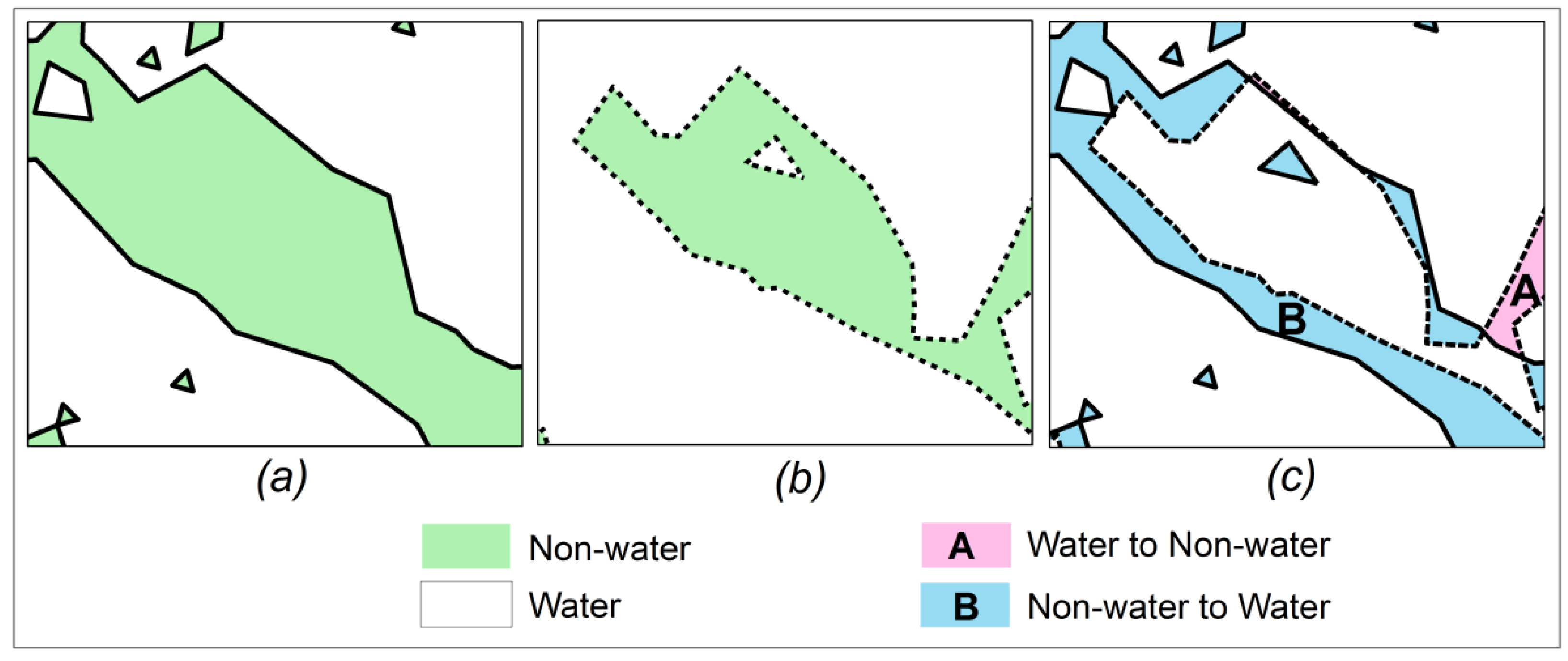
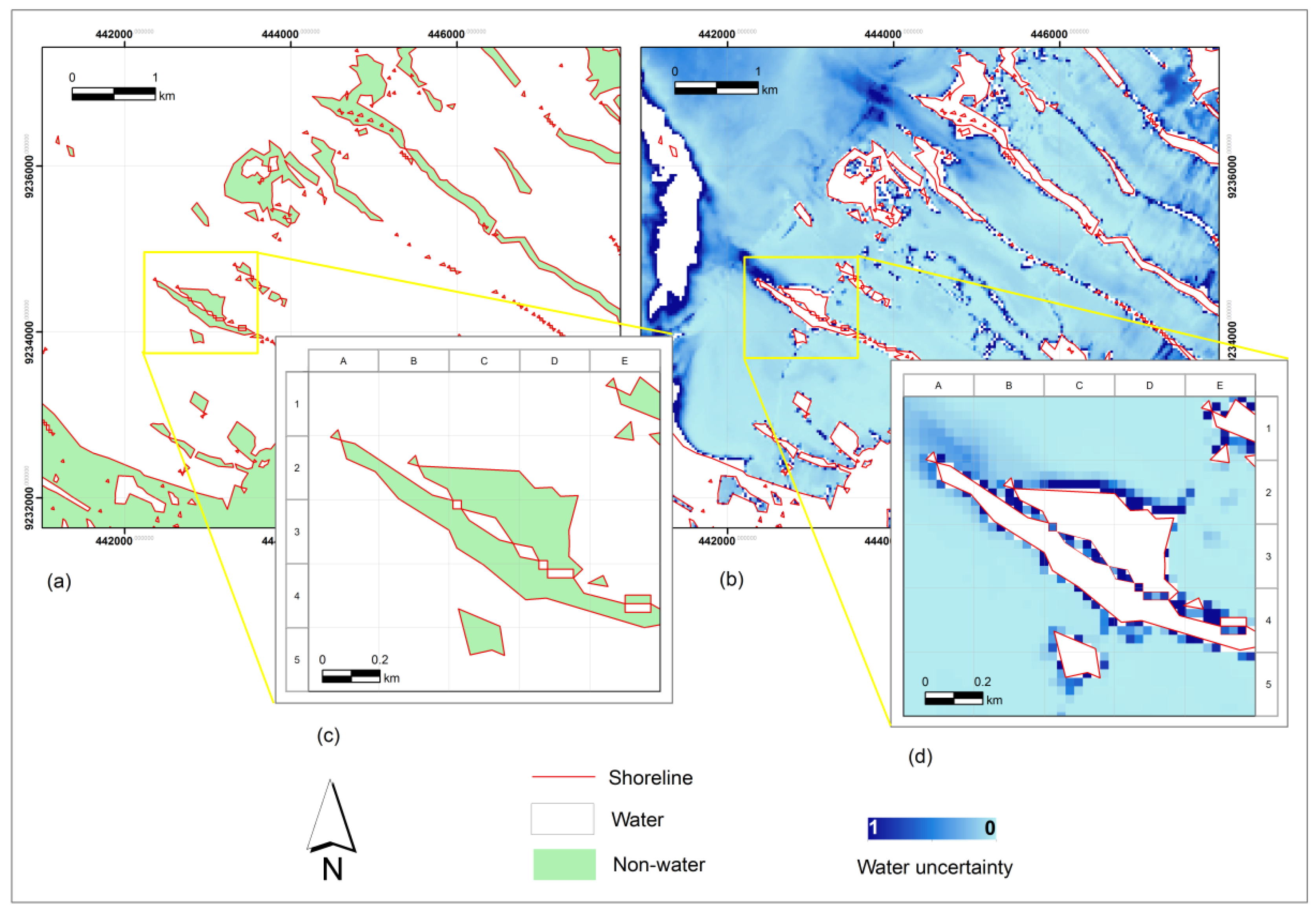
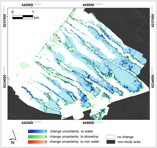
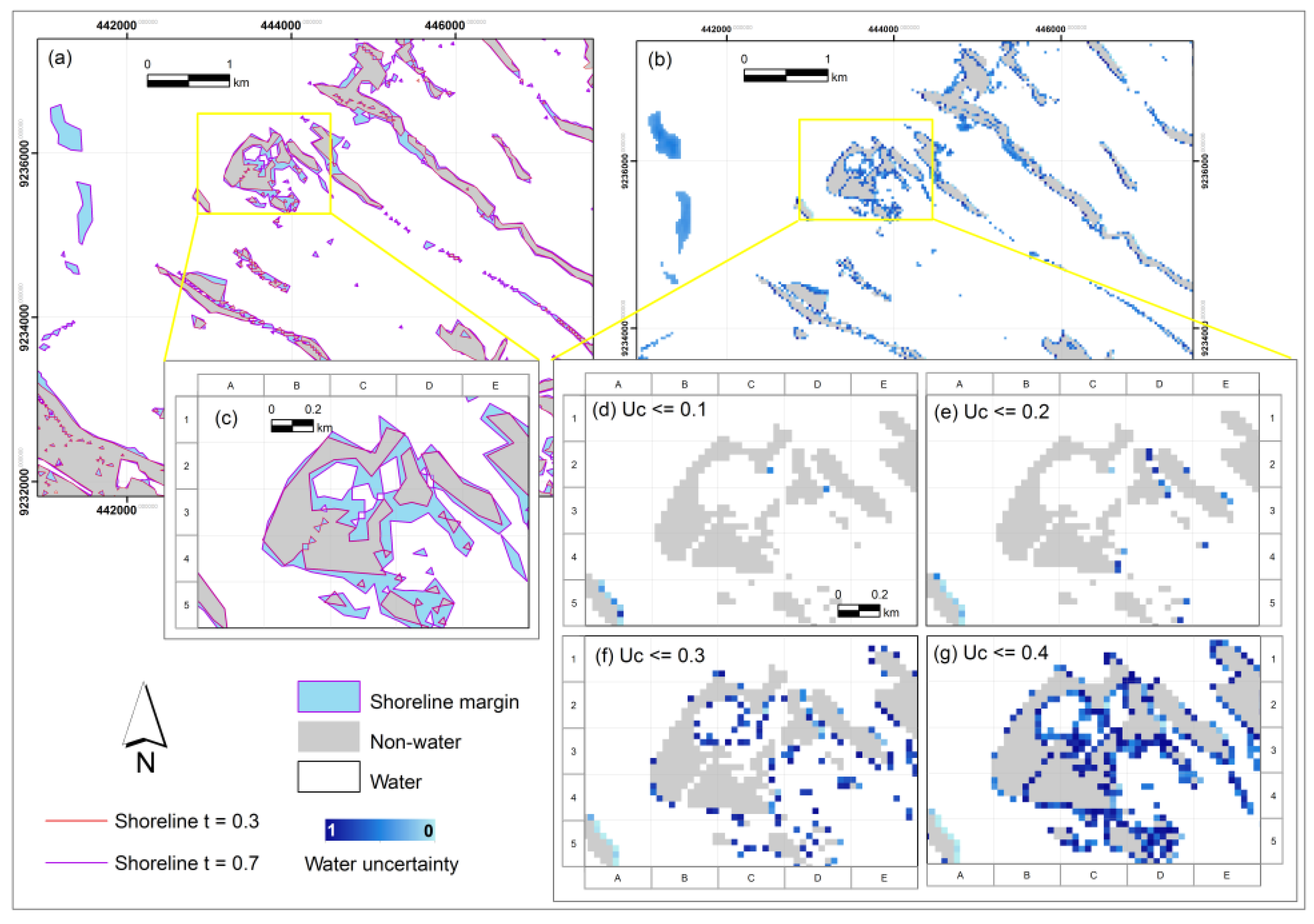
In this paper, we have demonstrated two change detection methods for shoreline considering its complex and fuzzy nature including its uncertainty. Both methods were successful in identifying abrupt and gradual changes of shoreline at an object level and in estimating the spatial distribution of uncertainty at the pixel level. 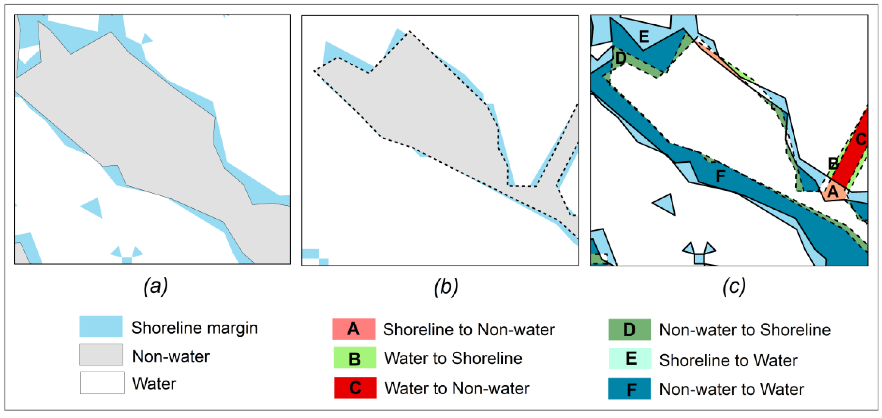The first method derived the shoreline by applying a threshold t = 0.5 on the water membership images. Shoreline was then considered as a single line; its position was influenced by the spatial extent of its associated sub-areas. The uncertainty in the shoreline position could be assessed by means of the uncertainty of its associated sub-areas. The second method derived shoreline margin as an area in which water moves to and fro as tides rise and fall. This margin was presented as a crisp object with a boundary determined by t values resulting from parameter estimation. Comparing these showed that the second method allowed us to assess the spatial extent of the shoreline and measure its change in uncertainty at different levels. 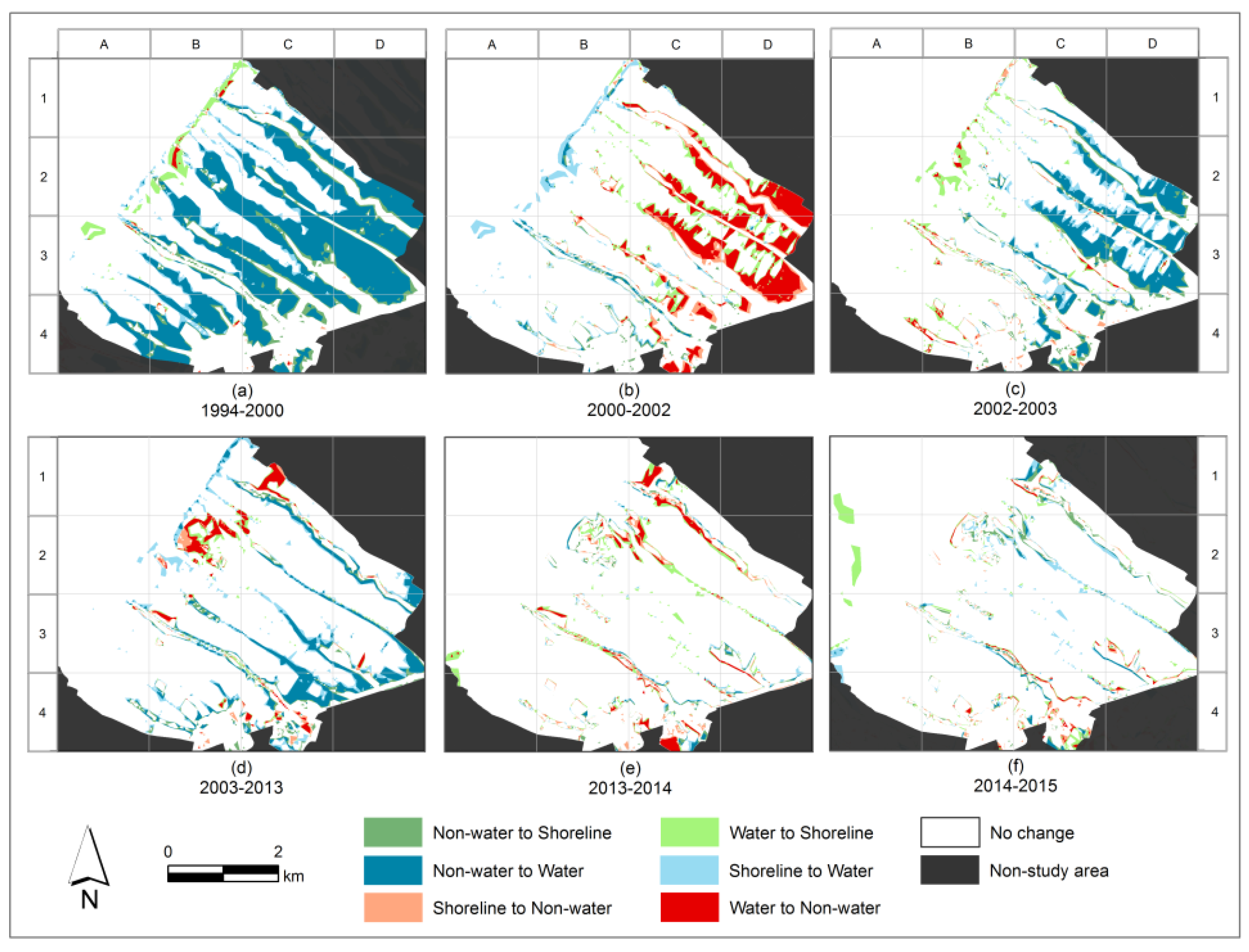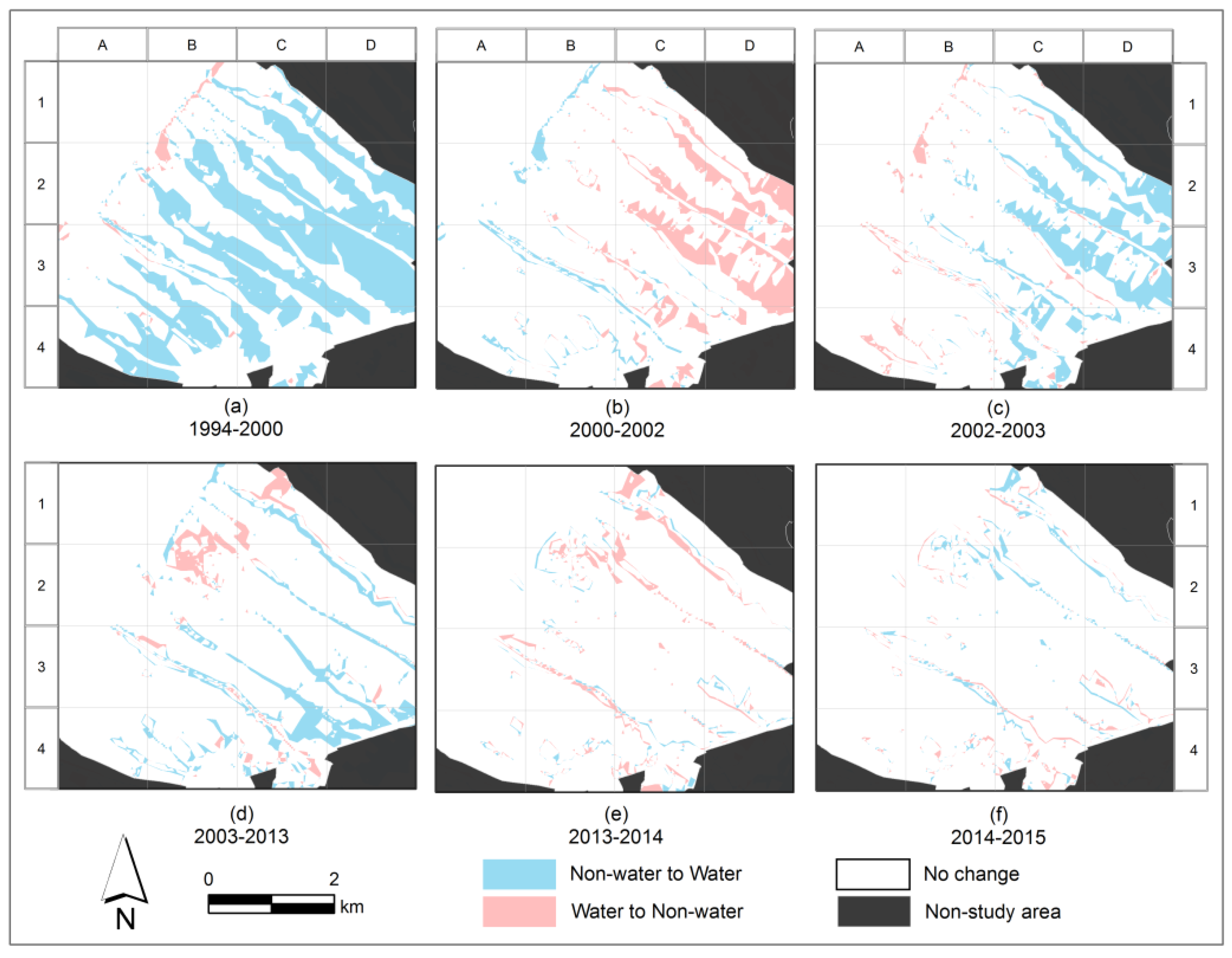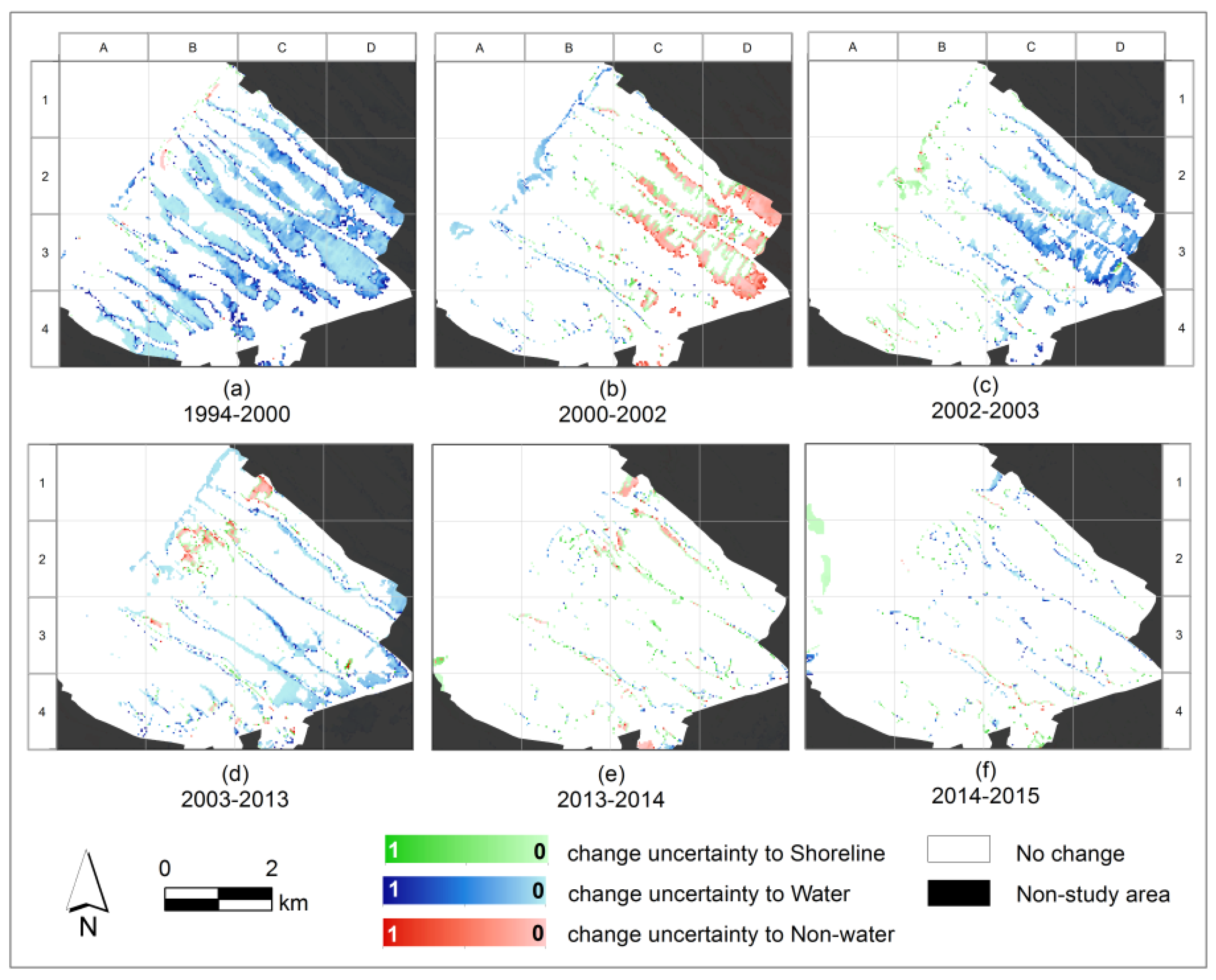This method provided more insight into the spatial distribution of changes and their uncertainty and more spatial detail of the process of change from non-water via shoreline margin to water and vice versa. In estimating the net change category, both methods gave similar results. 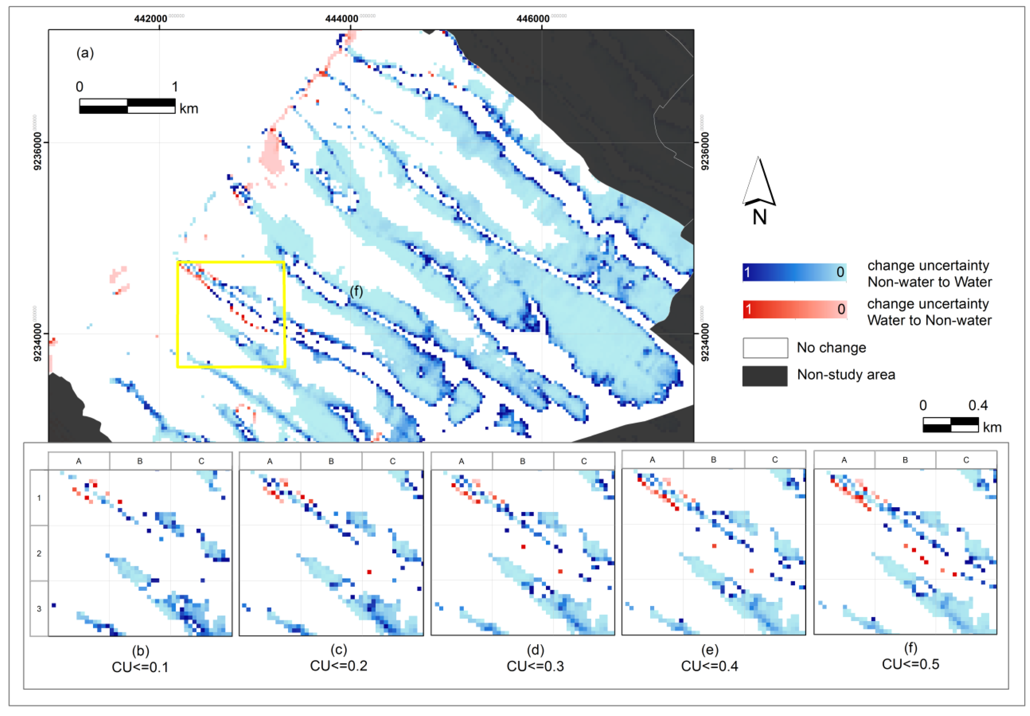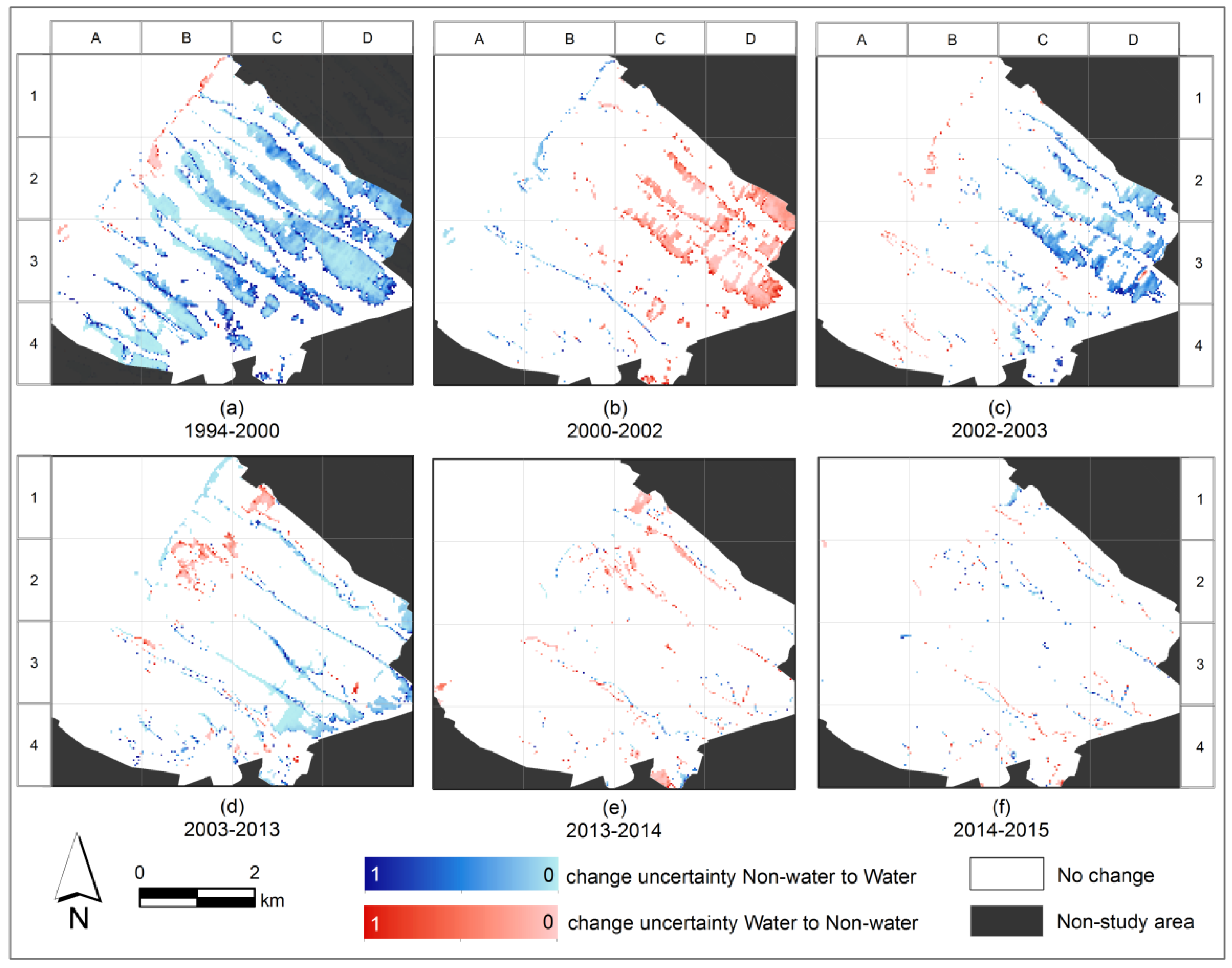Net changes identified by the second method covered a larger area both for negative changes (1994–2000, 2002–2003 and 2003–2013) as well as for positive changes (2000–2002 and 2013–2014), with the exception of 2014–2015 (see Table 5 and Table 7). The different results were mainly due to differences in threshold values when generating the shoreline. Shoreline and its changes have been presented as crisp sub-areas. The changed areas were thus associated with the distribution of change uncertainty.

In deriving shorelines as a fuzzy object, we used FCM to calculate the membership. Membership values obtained by applying FCM were used to deal with uncertain information on the position of objects, such as the location of fuzzy shorelines. In this research, we implemented FCM for two classes, since shoreline is the set of locations where water and non-water have physical interactions. In addition, the difference between water and non-water provided the largest spectral differences in images, as was confirmed in [52]. For similar situations, a suitable number of clusters need to be specified either by users based on their a priori knowledge or estimated from the images. In the literature, several methods exist to measure the cluster validity index for finding a suitable number of clusters, as for example exponential cluster validity index, non-fuzziness index, fuzziness performance index, and entropy measure [53,54,55,56].

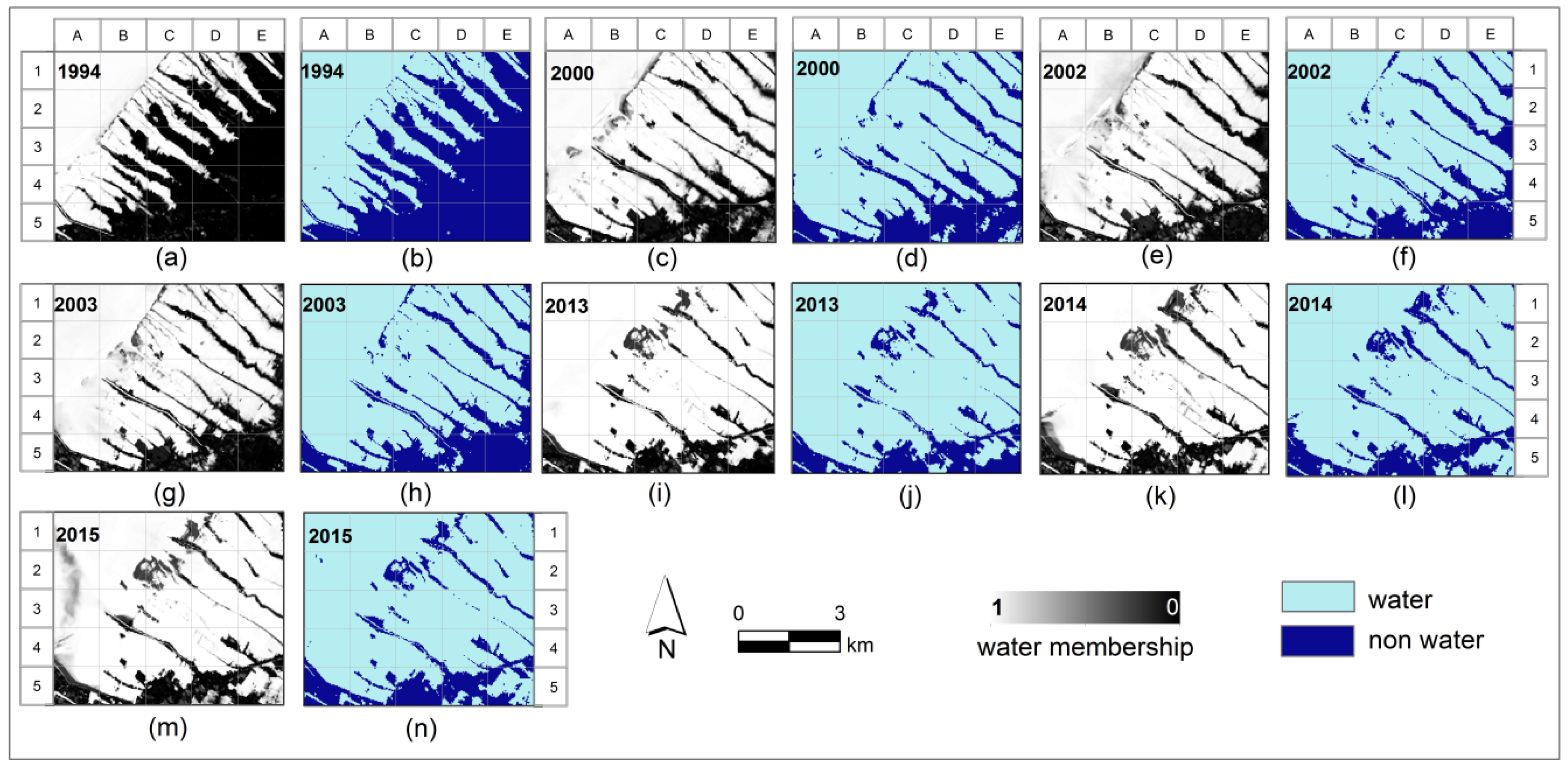
Reference data were collected in the field in 2015. In this research, images were selected based on the same low tide condition, and therefore, reference points were also selected under similar low tide conditions. Due to limited availability of high resolution images, however, the 2003 QuickBird image was used for accuracy assessment of images in 2000, 2002 and 2003, even though it was collected during rising tide. Differences in tides between images and these reference data have led to a low accuracy of classified images for 2000, 2002 and 2003, as compared to 2013 and 2015. Moreover, because of limited availability of Landsat images and severe cloud cover problems in the study area, other criteria such as availability of images with the same seasonal condition have not been applied yet. For images captured during rainy seasons, the rain increased the wetness of soil surfaces, which led to a false impression of more flooded conditions in the classified images, and increased the uncertainty in the shoreline position. Landsat images captured in 2000 and 2002 were recorded during the rainy seasons, while the 2003 QuickBird image, used as reference data, was captured during the dry season. Therefore, differences in seasons and tides could have contributed to the misclassification of water and non-water leading to lower classification accuracy. Considering the larger availability of new satellite images in the future, we recommend to select images recorded under similar, preferably dry, seasonal conditions to reduce the uncertainty due to seasonal influence.

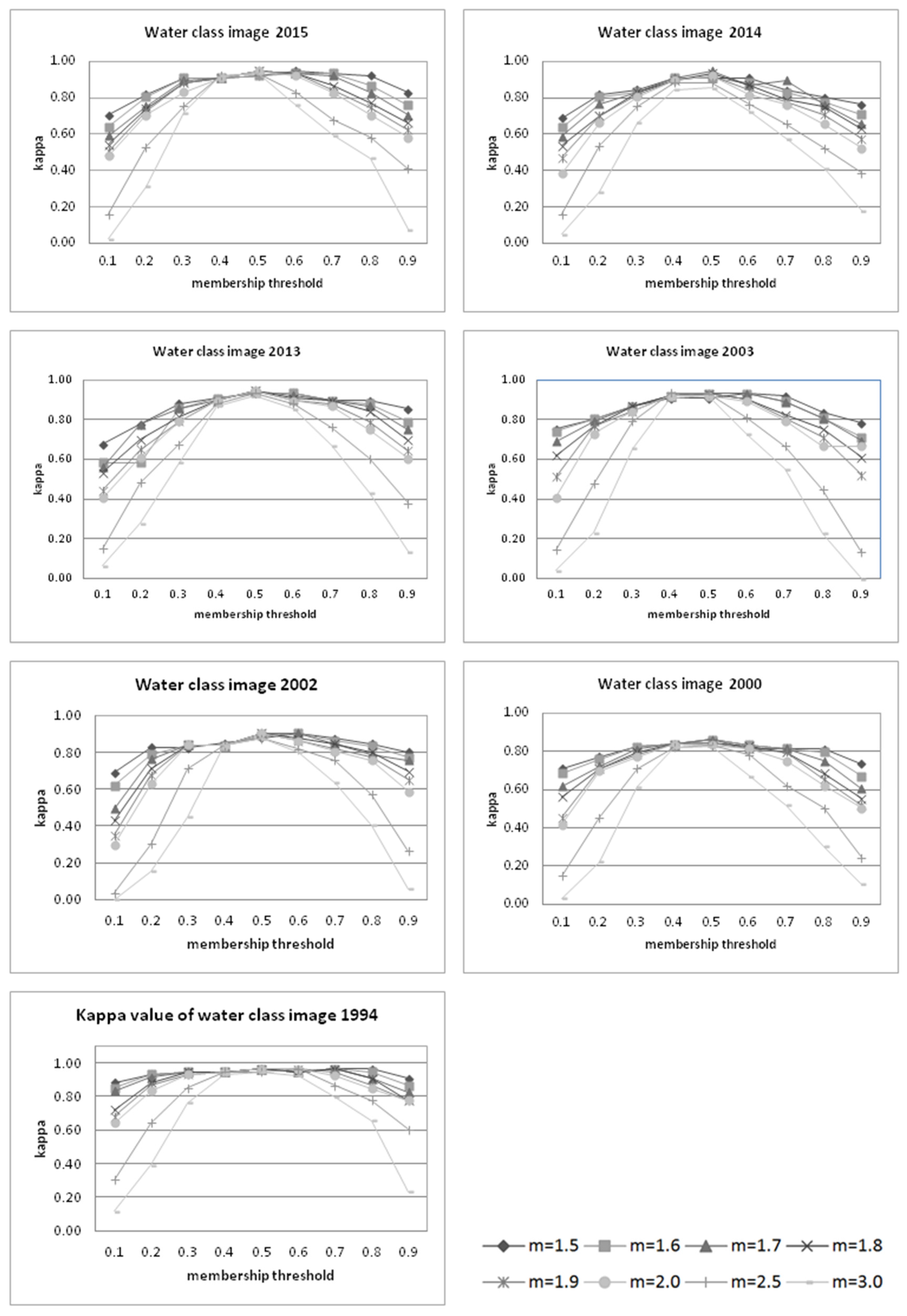
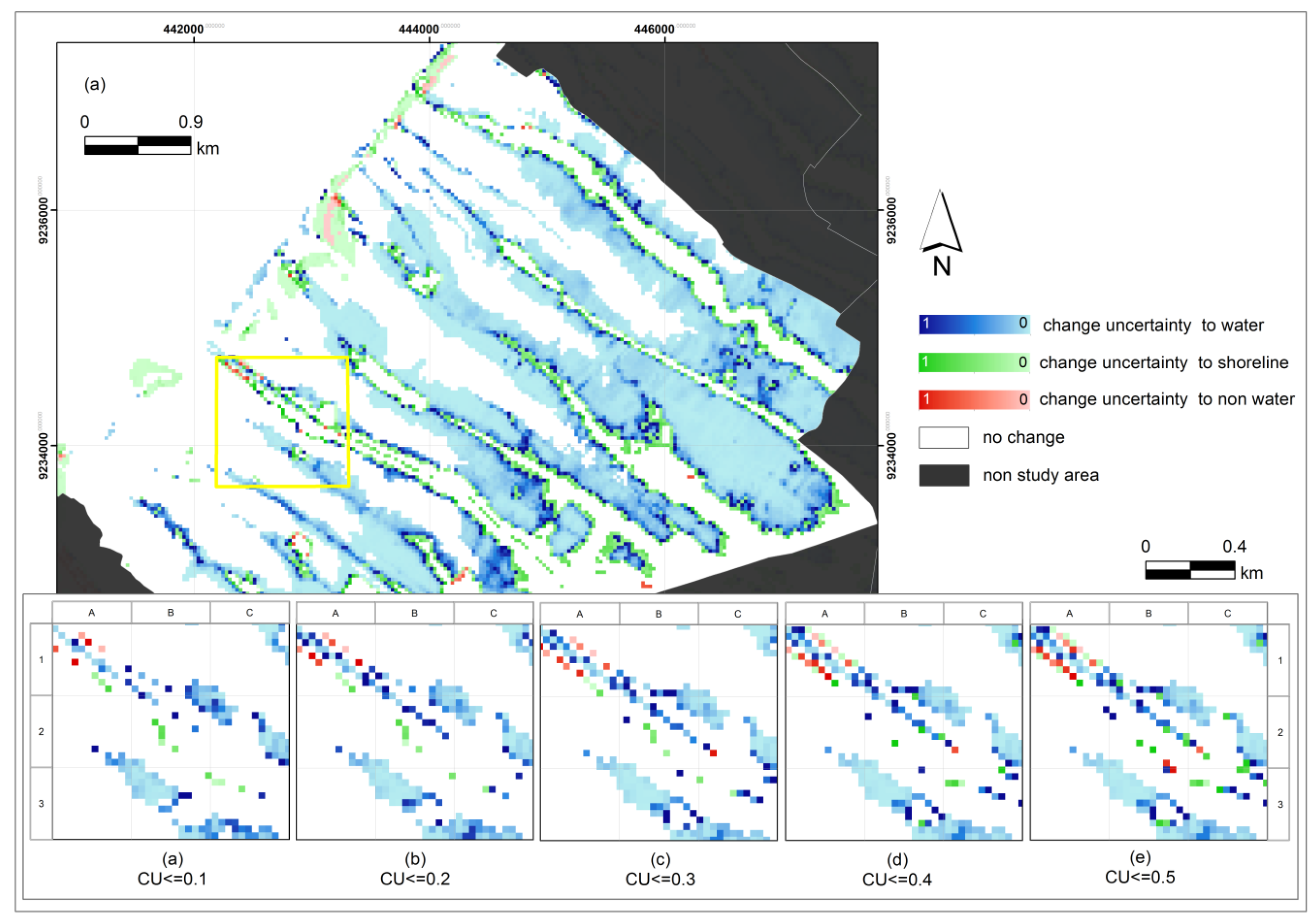
The shoreline change detection methods developed and applied in this research involved the generation of a shoreline and its uncertainty using selected m and t values, and produced a hard classification by means of thresholding. A variation in m values had little influence on the results of the classification. An important reason was the small changes in membership values obtained when m values were set between 1.5 and 3.0. Within that range, the change in membership value was generally less than 0.1. However, t variation strongly influenced the results. Small variations in t causing large variation in area indicate the presence of gradual boundaries, as for example in a muddy area. Meanwhile, sharp or sudden boundaries caused little change in area with varying t, such as at a steep coast or at the shoreline with embankment.

The change uncertainty value expresses how sure we are that a change really occurred. Therefore, the uncertainty addressed in this research corresponds to the existential uncertainty of the identified changes. A complete model of uncertainty, however, should also include an extensional uncertainty which considers the spatial extent of the change [57]. This would involve modelling shoreline as a fuzzy object as proposed by Cheng [51]. In fact, the membership and t values of the water class in this work may be used to represent shoreline as a conditional boundary since spatial extents of water (and non-water) depend on the choice of t value. In this case, points where $\mu =1$ are the interior of fuzzy sub-areas (cores), whereas points with $0<\mu <1$ would belong to transition zones and points with $\mu =0$ belong to non-water objects.

Analysis of shoreline changes in the study area in Sayung sub-district revealed an extensive change of shoreline with the largest change between 1994 and 2000. Land subsidence was indicated as one of the causes of this permanent submergence. Chaussard, et al. [58] mentioned that the rate of the land subsidence in this location reaches approximately 6.0 cm·year⁻¹. Subsidence was accelerated by an extreme ground water extraction for industrial purposes and as the consequence of a rapid population growth, classified as an anthropogenic subsidence. Putranto and Rüde [59] cited the Directorate of Environmental Geology and Mining Regions of Indonesia, stating the number of registered deep wells in Semarang Demak in the early 1900s was only 16. The number of deep wells increased significantly up to 1194 in 2002. Besides, land subsidence was also triggered by a natural compaction of clayey sediment and settlement loading [38,58,60]. Furthermore, the threat of flooding comes from sea level rise as well. As mentioned by Sofian [61], the rise of sea level in Indonesia is approximately 0.2–1.0 cm·year⁻¹ with an average of 0.6 cm·year⁻¹.

Different planting periods in agricultural areas could be a major cause of the changes from water and shoreline to non-water in the period 2000–2002 followed by a large reverse change in the period 2002–2003 (see Table 5 and Table 7). In addition, we identified coastal land reclamation activities to install an industrial area and a settlement in Sriwulan village. After the period 2003–2013, more agricultural areas were converted into fishponds as a result of expanding saltwater infiltration. On the other hand, some changes from water to non-water occurred as a result of a successful mangrove planting program which started in 2003.

The study area was located in a river delta formed from deposits carried by many rivers discharging into the Java Sea. The remarkable coastal inundation and erosion, which Sayung sub-district has faced for more than two decades, was probably also due to a change in sediment-carrying capacity of the longshore current [62,63]. This longshore current, generated by waves, exceeded the quantity of sediment supplied to the beach. Further, land use change in upstream areas resulted in an increase of erosion and water discharge in particular during rainy seasons, yielding more sediment to the downstream area. In fact, not all of this sediment could be discharged into the sea; some was deposited along the river bottom, irrigation canals, estuaries and other water bodies in its path. This led not only to the narrowing and to silting up of the canals and rivers, but also to the reduction of sediment supply to the littoral zone inducing coastal erosion. Moreover, massive coastal reclamation in a neighbouring area such as Terboyo industrial complex extended seaward after 1994, and Tanjung Emas Harbour first developed in 1985 could have changed currents and material transport along the coast in the study area as well. To prove that there were some influences of harbour development and beach reclamation to the severe inundation impact, however, is beyond the scope of this study.

5. Conclusions

This research presents two methods to identify shoreline positions: as a line and as a margin, including a measure of change uncertainty at different epochs. Both methods used FCM classification to determine partial membership of water and non-water. While shoreline changes can be detected by both methods, the shoreline as a margin provides a more detailed estimation of change area than the shoreline as a line. Moreover, by having shoreline as a margin, we can assess its spatial extent and measure its change uncertainty at different levels. Abrupt and gradual changes of shoreline were identified at an object level and the spatial distribution of uncertainty estimated at a pixel level.

Some challenges for the improvement of the method consist of: (1) including an extensional uncertainty and represent shoreline as a conditional boundary; (2) including seasonal condition in the selection of images; and (3) integrating the results with a digital elevation model. In addition, the integration with other datasets such as land use and land cover pattern, hydrological data and other information associated with the study area is important as well to have a better understanding of processes which influence the shoreline change.

Both methods have been successfully implemented in a coastal area in the Sayung sub-district in Java using a series of Landsat images. The change area estimation and its change uncertainty may support local government and other stakeholders in monitoring shoreline changes. Integrating the results with the distribution of elements at risk such as settlements and other important facilities can help to analyze which location needs to be prioritized in disaster response. For example, priority could be given to a change area from shoreline to water which has low change uncertainty value as it was obvious that shoreline has changed due to inundation or erosion. Priority could also be given, however, to the area with higher change uncertainty, for example if the location is a densely populated area. Continuous monitoring of shoreline changes in order to understand risks and to anticipate the potential impacts is highly important.

References

1. Vaidya, A.M.; Kori, S.K.; Kudale, M.D. Shoreline response to coastal structures. Aquat. Procedia 2015, 4, 333–340. [Google Scholar] [CrossRef]
2. Ali, T.A. Analysis of shoreline-changes based on the geometric representation of the shorelines in the GIS database. J. Geogr. Geospat. Inf. Sci. 2010, 1, 1–16. [Google Scholar]
3. Li, R.; Ma, R.; Di, K. Digital tide-coordinated shoreline. Mar. Geod. 2002, 25, 27–36. [Google Scholar] [CrossRef]
4. Klemas, V. Beach profiling and LiDAR bathymetry: An overview with case studies. J. Coast. Res. 2011, 27, 1019–1028. [Google Scholar] [CrossRef]
5. Dolan, R.; Fenster, M.S.; Holme, S.J. Temporal analysis of shoreline recession and accretion. J. Coast. Res. 1991, 31, 1819–1836. [Google Scholar]
6. Dean, R.G.; Dalrymple, R.A. Coastal Processes: With Engineering Applications; Cambridge University Press: Cambridge, UK, 2002; p. 473. [Google Scholar]
7. Bird, E.C.F. Coastline Changes: A Global Review; John Wiley and Sons: Hoboken, NJ, USA, 1985; p. 219. [Google Scholar]
8. Boak, E.H.; Turner, I.L. Shoreline definition and detection: A review. J. Coast. Res. 2005, 21, 688–703. [Google Scholar] [CrossRef]
9. Davidson-Arnott, R. An Introduction to Coastal Processes and Geomorphology; Cambridge University Press: Cambridge, UK, 2010; p. 442. [Google Scholar]
10. Oertel, G.F. Coasts, coastlines, shores, and shorelines. In Encyclopedia of Coastal Science; Schwartz, M.L., Ed.; Springer: Berlin, Germany; Heidelberg, Germany, 2005; pp. 323–327. [Google Scholar]
11. Gens, R. Remote sensing of coastlines detection, extraction and monitoring. Int. J. Remote Sens. 2010, 31, 1819–1836. [Google Scholar] [CrossRef]
12. Leatherman, S.P.; Eskandary, L.S. Evaluation of coastal erosion hazards along Delaware’s Atlantic coast. J. Coast. Res. 1999, SI, 43–49. [Google Scholar]
13. Gorman, L.; Morang, A.; Larson, R. Monitoring the coastal environment; part IV: Mapping, shoreline changes, and bathymetric analysis. J. Coast. Res. 1998, 14, 61–92. [Google Scholar]
14. Chen, W.W.; Chang, H.K. Estimation of shoreline position and change from satellite images considering tidal variation. Estuar. Coast. Shelf Sci. 2009, 84, 54–60. [Google Scholar] [CrossRef]
15. Ghosh, M.K.; Kumar, L.; Roy, C. Monitoring the coastline change of Hatiya Island in Bangladesh using remote sensing techniques. ISPRS J. Photogramm. 2015, 101, 137–144. [Google Scholar] [CrossRef]
16. Wang, Y. Using Landsat 7 TM data acquired days after a flood event to delineate the maximum flood extent on a coastal floodplain. Int. J. Remote Sens. 2004, 25, 959–974. [Google Scholar] [CrossRef]
17. Dewan, A.M.; Yamaguchi, Y. Effect of land cover changes on flooding: Example from greater Dhaka of Bangladesh. Int. J. Geoinform. 2008, 4, 11–19. [Google Scholar]
18. Senthilnatha, J.; Shenoy, H.V.; Omkar, S.N.; Mani, V. Spectral-spatial MODIS image analysis using swarm intelligence algorithms and region based segmentation for flood assessment. In Proceedings of the 7th International Conference on Bio-Inspired Computing: Theories and Applications; Bansal, J.C., Singh, P.K., Deep, K., Pant, M., Nagar, A.K., Eds.; Springer: Berlin, Germany; Heidelberg, Germany, 2012. [Google Scholar]
19. Martinis, S.; Twele, A.; Strobl, C.; Kersten, J.; Stein, E. A multi-scale flood monitoring system based on fully automatic MODIS and TerraSAR-X processing chains. Remote Sens. 2013, 5, 5598–5619. [Google Scholar] [CrossRef]
20. Ouma, Y.O.; Tateishi, R. A water index for rapid mapping of shoreline changes of five East African Rift Valley Lakes: An empirical analysis using Landsat TM and ETM+ Data. Int. J. Remote Sens. 2007, 27, 3153–3181. [Google Scholar] [CrossRef]
21. Tamassoki, E.; Amiri, H.; Soleymani, Z. Monitoring of shoreline changes using remote sensing (case study: coastal city of Bandar Abbas). In Proceedings of the 7th IGRSM International Remote Sensing & GIS Conference and Exhibition, Kuala Lumpur, Malaysia, 21–22 April 2014; IOP Publishing: Kuching, Malaysia, 2014; Volume 20. [Google Scholar]
22. Li, X.; Damen, M.C.J. Coastline change detection with satellite remote sensing for environmental management of the Pearl River Estuary, China. J. Mar. Syst. 2010, 82, S54–S61. [Google Scholar] [CrossRef]
23. Ford, M. Shoreline changes interpreted from multi-temporal aerial photographs and high resolution satellite images: Wotje Atoll, Marshall Islands. Remote Sens. Environ. 2013, 135, 130–140. [Google Scholar] [CrossRef]
24. Marfai, M.A.; Almohammad, H.; Dey, S.; Susanto, B.; King, L. Coastal dynamic and shoreline mapping: multi-sources spatial data analysis in Semarang Indonesia. Environ. Monit. Assess. 2008, 142, 297–308. [Google Scholar] [CrossRef] [PubMed]
25. Muslim, A.M.; Foody, G.M.; Atkinson, P.M. Localized soft classification for super-resolution mapping of the shoreline. Int. J. Remote Sens. 2006, 27, 2271–2285. [Google Scholar] [CrossRef]
26. Taha, L.G.E.D.; Elbeih, S.F. Investigation of fusion of SAR and Landsat data for shoreline super resolution mapping: The Northeastern Mediterranean sea coast in Egypt. Appl. Geomat. 2010, 2, 177–186. [Google Scholar] [CrossRef]
27. Yao, F.; Parrish, C.E.; Pe’eri, S.; Calder, B.R.; Rzhanov, Y. Modeling uncertainty in photogrammetry-derived national shoreline. Mar. Geod. 2015, 38, 128–145. [Google Scholar] [CrossRef]
28. Río, L.D.; Gracia, F.J. Error determination in the photogrammetric assessment of shoreline changes. Nat. Hazards 2013, 65, 2385–2397. [Google Scholar]
29. Genz, A.S.; Fletcher, C.H.; Dunn, R.A.; Frazer, L.N.; Rooney, J.J. The predictive accuracy of shoreline change rate methods and alongshore beach variation on Maui, Hawaii. J. Coast. Res. 2007, 23, 87–105. [Google Scholar] [CrossRef]
30. Maiti, S.; Bhattacharya, A.K. Shoreline change analysis and its application to prediction: A remote sensing and statistics based approach. Mar. Geol. 2009, 257, 11–23. [Google Scholar] [CrossRef]
31. Bezdek, J.C.; Ehrlich, R.; Full, W. FCM: The fuzzy c-means clustering algorithm. Comput. Geosci. 1984, 10, 191–203. [Google Scholar] [CrossRef]
32. Hartini, S. Flood Risk Modelling on Agricultural Area in the North Coastal Area of Central Java. Ph.D. Dissertation, Gadjah Mada University, Yogyakarta, Indonesia, 2015. [Google Scholar]
33. Marfai, M.A. Preliminary assessment of coastal erosion and local community adaptation in Sayung coastal area, Central Java—Indonesia. Quaest. Geogr. 2012, 31, 47–55. [Google Scholar]
34. Harwitasari, D.; van Ast, J.A. Climate change adaptation in practice: People’s responses to tidal flooding in Semarang, Indonesia. J. Flood Risk Manag. 2011, 4, 216–233. [Google Scholar] [CrossRef]
35. Marfai, M.A.; King, L.; Sartohadi, J.; Sudrajat, S.; Budiani, S.R.; Yulianto, F. The impact of tidal flooding on a coastal community in Semarang, Indonesia. Environmentalist 2008, 28, 237–248. [Google Scholar] [CrossRef]
36. Sarbidi. Rob influence on coastal settlements (case study: Semarang city). In Proceedings of the Losses in Buildings and Areas Due Sea-level Rise on Coastal Cities in Indonesia, Bandung, Indonesia, 19–20 March 2001; Research Center for Settlements, Ministry of Public Works: Bandung, Indonesia, 2001. [Google Scholar]
37. Kurniawan, L. Tidal flood assessment in Semarang (case: Dadapsari). Alami. 2003, 8, 54–59. Available online: http://ejurnal.bppt.go.id/index.php/alami/article/view/1041 (accessed on 8 June 2015). [Google Scholar]
38. Marfai, M.A.; King, L. Tidal inundation mapping under enhanced land subsidence in Semarang, Central Java Indonesia. Nat. Hazards 2008, 44, 93–109. [Google Scholar] [CrossRef]
39. Winterwerp, H.; van Wesenbeeck, B.; van Dalfsen, J.; Tonneijck, F.; Astra, A.; Verschure, S.; van Eijk, P. A Sustainable Solution for Massive Coastal Erosion in Central Java; Discussion Paper; Deltares–Wetland International: Wageningen, The Netherlands, 2014; p. 45. Available online: http://www.wetlands.org/LinkClick.aspx?fileticket=rv2jbvHx%2bHw%3d&tabid=56 (accessed on 13 July 2015).
40. Hadjimitsis, D.G.; Papadavid, G.; Agapiou, A.; Themistocleous, K.; Hadjimitsis, M.G.; Retalis, A.; Michaelides, S.; Chrysoulakis, N.; Toulios, L.; Clayton, C.R.I. Atmospheric correction for satellite remotely sensed data intended for agricultural applications: Impact on vegetation indices. Nat. Hazards Earth Syst. Sci. 2010, 10, 89–95. [Google Scholar] [CrossRef]
41. Mather, P.M. Computer Processing of Remotely-Sensed Images: An Introduction, 3rd ed.; John Wiley & Sons: Chicester, UK, 2004; p. 352. [Google Scholar]
42. Foody, G. Approaches for the production and evaluation of fuzzy land cover classifications from remotely-sensed data. Int. J. Remote Sens. 1996, 17, 1317–1340. [Google Scholar] [CrossRef]
43. Richards, J.A. Remote Sensing Digital Image Analysis, 5th ed.; Springer: Berlin/Heidelberg, Germany, 2013. [Google Scholar]
44. Li, M.; Stein, A.; Bijker, W.; Zhan, Q. Region-based urban road extraction from VHR satellite images using binary partition tree. Int. J. Appl. Earth Observ. Geoinf. 2015, 44, 217–225. [Google Scholar]
45. Sebari, I.; He, D.C. Automatic fuzzy object-based analysis of VHSR images for urban objects extraction. ISPRS J. Photogramm. 2013, 79, 171–184. [Google Scholar]
46. Dubois, D.; Esteva, F.; Godo, L.; Prade, H. Fuzzy-set based logics—An history-oriented presentation of their main developments. In Handbook of the History of Logic; Gabbay, D.M., Woods, J., Eds.; Elsevier: Amsterdam, The Netherlands, 2007; Volume 8, pp. 325–449. [Google Scholar]
47. Zadeh, L.A. PRUF a meaning representation language for natural languages. Int. J. Mach. Stud. 1978, 10, 395–460. [Google Scholar]
48. Lu, D.; Li, G.; Moran, E. Current situation and needs of change detection techniques. Int. J. Image Data Fusion 2014, 5, 13–38. [Google Scholar] [CrossRef]
49. Egenhofer, M.J.; Al-Taha, K.K. Reasoning about gradual changes of topological relationships. In Theories and Methods of Spatio-Temporal Reasoning in Geographic Space; Frank, A.U., Campari, I., Formentini, U., Eds.; Springer: Berlin/Heidelberg, Germany, 1992. [Google Scholar]
50. Ardila, J.P.; Bijker, W.; Tolpekin, V.A.; Stein, A. Quantification of crown changes and change uncertainty of trees in an urban environment. ISPRS J. Photogramm. 2012, 74, 41–55. [Google Scholar]
51. Cheng, T. A Process-Oriented Data Model for Fuzzy Spatial Objects. Ph.D. Dissertation, ITC-Wageningen University, Wageningen, The Netherlands, 1999. [Google Scholar]
52. Bijker, W.; Hamm, N.A.; Ijumulana, J.; Wole, M.K. Monitoring a fuzzy object: The case of Lake Naivasha. In Proceedings of the 6th International Workshop on the Analysis of Multi-temporal Remote Sensing Images (Multi-Temp), Trento, Italy, 12–14 July 2011.
53. Zarandi, M.H.F.; Faraji, M.R.; Karbasian, M. An exponential cluster validity index for fuzzy clustering with crisp and fuzzy data. Sci. Iran. Trans. E Ind. Eng. 2010, 17, 95–110. [Google Scholar]
54. Tso, B.; Mather, P. Classification Methods for Remotely Sensed Data; CRC Press: Boca Raton, FL, USA, 2009; p. 347. [Google Scholar]
55. Fisher, P.F.; Pathirana, S. The evaluation of fuzzy membership of land cover classes in the suburban zone. Remote Sens. Environ. 1990, 34, 121–132. [Google Scholar] [CrossRef]
56. Roubens, M. Fuzzy clustering algorithms and their cluster validity. Eur. J. Oper. Res. 1982, 10, 294–301. [Google Scholar] [CrossRef]
57. Molenaar, M.; Cheng, T. Fuzzy spatial objects and their dynamics. ISPRS J. Photogramm. 2000, 55, 164–175. [Google Scholar] [CrossRef]
58. Chaussard, E.; Amelung, F.; Abidin, H.; Hong, S.H. Sinking cities in Indonesia: ALOS PALSAR detects rapid subsidence due to groundwater and gas extraction. Remote Sens. Environ. 2013, 128, 150–161. [Google Scholar] [CrossRef]
59. Putranto, T.T.; Rüde, T.R. Groundwater Problem in Semarang Demak Urban Area, Java/Indonesia. Available online: http://geostat-course.org/node/857 (accessed on 18 July 2015).
60. Lubis, A.M.; Sato, T.; Tomiyama, N.; Isezaki, N.; Yamanokuchi, T. Ground subsidence in Semarang-Indonesia investigated by ALOS–PALSAR satellite SAR interferometry. J. Asian Earth Sci. 2011, 40, 1079–1088. [Google Scholar] [CrossRef]
61. Sofian, I. Scientific Basis: Analysis and Projection of Sea Level Rise and Extreme Event; National Development Planning Agency: Bappenas, Indonesia, 2010; p. 70. [Google Scholar]
62. Office of the Mayor of Semarang City. The Master Plan of Drainage System of Semarang; Office of the Mayor of Semarang City: City of Semarang, Indonesia, 2014; Volume 7, p. 45. [Google Scholar]
63. Astra, A.S.; Sabarini, E.K.; Harjo, A.M.; Maulana, M.B. Mangrove-based and community-based coastal protection in Timbulsloko village, Demak. In Wetland Conservation Magazine; Wetlands International Indonesia: Bogor, Indonesia, 2014; pp. 4–5. [Google Scholar]
Figure 1. The study area in Sayung sub-district, Central Java Province covering four coastal villages. The RGB 532 of Landsat image 2015 is displayed as the background. A severe coastal inundation was reported leading to a large shoreline change.
Remotesensing 08 00190 g001
Figure 2. Some examples of the impact of coastal inundation: (a) daily floods at the house yard; (b) an abandoned fish landing facility (the red dashed line shows the previous shoreline), (c) permanent inundation of several houses.
Remotesensing 08 00190 g002
Figure 3. (ad) The comparison of normal (a,c) and flooded (b,d) situations due to coastal inundation at two locations at Sayung sub-district. Over a longer period, this cyclic flood leads to a permanent inundation.
Remotesensing 08 00190 g003
Figure 4. Trapezoidal membership function. Area between b and c is a core zone which has a membership value equal to 1 to the water class. Area a-b and c-d are transition zones or boundaries which have value between 0 and 1 to the water class, while the pixels with 0 memberships do not belong to the water class.
Remotesensing 08 00190 g004
Figure 5. (ah) Topological relationships between two sub-areas. Green polygons represent sub-area R T 1 and blue polygons represent sub-area R T 2 .
Remotesensing 08 00190 g005
Figure 6. (a) Shoreline at time T 1 ; (b) Shoreline at time T 2 ; (c) Shoreline change estimation considering two categories of changed areas, namely: (A) water to non-water, and (B) non-water to water. Solid lines represent shoreline at T 1 whereas dashed lines refer to shoreline at T 2 .
Remotesensing 08 00190 g006
Figure 7. (a) Shoreline margin at time T 1 ; (b) Shoreline margin at time T 2 ; (c) Shoreline change estimation considering six changed areas, namely: (A) shoreline to non-water, (B) water to shoreline, (C) water to non-water, (D) non-water to shoreline, (E) shoreline to water, and (F) non-water to water. Solid lines represent shoreline margins at T 1 whereas dashed lines refer to shoreline margins at T 2 .
Remotesensing 08 00190 g007
Figure 8. The accuracy assessment results of water class images, generated by applying FCM classification followed by thresholding on the water membership image. The highest kappa (κ) values were obtained from t = 0.5 for all images, and t = 0.3 and 0.7 gave a nearly constant κ value.
Remotesensing 08 00190 g008
Figure 9. (an) FCM results show the membership of water class (a,c,e,g,i,k,m), and classified images of water class by setting t = 0.5 (b,d,f,h,j,l,n). The shrinking of non-water sub-areas over two decades can be identified by the change of the shape of the non-water class from wide strips to the thin elongated shapes over the series of images (see (an); e.g., grid cells C3). Whereas non-water sub-areas emerged when mangroves were planted (see (i) grid cells C2), and in coastal reclamation areas (see (a,c) grid cells A5).
Remotesensing 08 00190 g009
Figure 10. (ad) The illustration of shoreline as a line; (a) Shorelines (in red colour) created by setting t = 0.5; (b) the uncertainty of pixels classified as water at the uncertainty level ≤0.5. Generally, pixels closer to the shoreline have a higher uncertainty value (see (d) grid cells C2 and D2).
Remotesensing 08 00190 g010
Figure 11. The illustration of shoreline as a margin; (a) Shoreline margin (blue polygons) generated by giving t = 0.3 and 0.7 ; (b) the uncertainty of shoreline margin from Equation (12); (c) zooming in sub-areas in yellow rectangle based on Figure 11a. Shoreline margin was assessed through different levels of uncertainty ( U C ): (d) ≤0.1; (e) ≤0.2; (f) ≤0.3; and (g) ≤0.4.
Remotesensing 08 00190 g011
Figure 12. (af) Shoreline change analysis at t = 0.5. Two changes were identified, namely non-water to water and water to non-water. Large areas changed from non-water to water such as due to inundation and erosion which were indicated between 1994 and 2000 (a). Whereas large areas changed from water to non-water and were distinguished between 2000 and 2002 (b).
Remotesensing 08 00190 g012
Figure 13. (a) Shoreline change uncertainty at t = 0.5; (bf) Change uncertainty is highlighted at different levels for the period 1994–2000 for the yellow rectangle site. The number of red pixels indicates that the change uncertainty from water to non-water increase with the increase of uncertainty values, as also can be seen for the blue pixels.
Remotesensing 08 00190 g013
Figure 14. (af) Shoreline change uncertainty at t = 0.5 and CU ≤ 0.1 for the period 1994–2015. The extensive inundation has been indicated from 1994 to 2000 (a) and the largest change to non-water occurred in the period 2000–2002 (b).
Remotesensing 08 00190 g014
Figure 15. (af) The changes of shoreline margin, water and non-water. Six changes were identified including abrupt and gradual changes. An extensive inundation has been indicated from 1994 to 2000 (a), while the large change to non-water occurred in the period 2000–2002 (b).
Remotesensing 08 00190 g015
Figure 16. (a) Shoreline change uncertainty for the period 1994–2000; (bf) Change uncertainty was measured at different levels for yellow rectangle site. A number of pixels (red, green, and blue) increase with the increase in the level of uncertainty. Changes from non-water to shoreline and from water to shoreline were grouped under one label and are presented in shades of green, while changes from shoreline and water to non-water are presented in shades of red. Changes from non-water and shoreline to water are represented as shades of blue.
Remotesensing 08 00190 g016
Figure 17. (af) Change uncertainty of shoreline margins and their associated sub-areas at CU level ≤ 0.1 in the period 1994–2015. (a) The largest coastal inundation occurred in the period 1994–2000. It was dominated by light blue pixels indicated low change uncertainty values to water; (b) The largest increase in non-water occurred in the period 2000–2002 represented by light red pixels indicated low change uncertainty to non-water.
Remotesensing 08 00190 g017