Study of the Effect of Temporal Sampling Frequency on DSCOVR Observations Using the GEOS-5 Nature Run Results (Part I): Earth’s Radiation Budget

Abstract

Satellites always sample the Earth-atmosphere system in a finite temporal resolution. This study investigates the effect of sampling frequency on the satellite-derived Earth radiation budget, with the Deep Space Climate Observatory (DSCOVR) as an example. The output from NASA’s Goddard Earth Observing System Version 5 (GEOS-5) Nature Run is used as the truth. The Nature Run is a high spatial and temporal resolution atmospheric simulation spanning a two-year period. The effect of temporal resolution on potential DSCOVR observations is assessed by sampling the full Nature Run data with 1-h to 24-h frequencies. The uncertainty associated with a given sampling frequency is measured by computing means over daily, monthly, seasonal and annual intervals and determining the spread across different possible starting points. The skill with which a particular sampling frequency captures the structure of the full time series is measured using correlations and normalized errors. Results show that higher sampling frequency gives more information and less uncertainty in the derived radiation budget. A sampling frequency coarser than every 4 h results in significant error. Correlations between true and sampled time series also decrease more rapidly for a sampling frequency less than 4 h.

1. Introduction

Satellite remote sensing remains the only feasible way of observing the Earth on a global scale. Geophysical parameters retrieved from satellite observations have been playing a critical role in studying the Earth-atmosphere system. The Deep Space Climate Observatory (DSCOVR) is particularly well suited for providing such observations. Orbiting around the Sun-Earth L1 Lagrange point, a location where gravitational and centrifugal forces are in balance for an orbital period equal to Earth’s, the DSCOVR satellite always stays near the Sun-Earth line. In this position, which lies around 1.5 million km away from the Earth, DSCOVR can view the entire daytime hemisphere continuously. DSCOVR is equipped with two Earth-observing instruments: the National Institute of Standards and Technology Advanced Radiometer (NISTAR) and the Earth Polychromatic Imaging Camera (EPIC) [1]. NISTAR views the Earth as one pixel and provides broadband radiation information about the Earth and its atmosphere. EPIC images the Earth with 10 spectral channels ranging from the ultraviolet to the near infrared with it 2048 by 2048 CCD array. Combined information from the two instruments will be used to derive the Earth’s radiation budget, as well as ozone, cloud, aerosol and vegetation properties.

DSCOVR, like any other satellite, can only provide observations with a finite temporal resolution. As a result, the information derived from these observations is a subsample of the true system. In general, subsampling will affect the accuracy of the retrieved results [2,3]. For this study, the focus is on clouds and radiation budget. The specific questions to be addressed include: how does subsampling affect the mean, and how close is the sampled time series to the truth? This paper presents the analysis of the temporal sampling effect on Earth’s radiation budget; analysis with cloud cover will be presented in Part 2.

To truly study the effect of temporal sampling frequency, a truth dataset with an infinitesimal sampling rate would be required in order to capture the constantly changing scene underneath the spacecraft, yet this is not practical. Instead, the output from a global atmospheric model is used. This provides the best substitute for a continuous dataset. NASA produces operational weather forecasts using the Goddard Earth Observing System Version 5 (GEOS-5). Recently, a very high spatial and temporal resolution version of GEOS-5 was run in a free-running climate-like simulation. In this so-called Nature Run mode, a convection resolving horizontal resolution was used with a model time step of a few minutes; the total integration time is just over two years. Much effort has gone into validating the Nature Run [4], and it has been shown to have very realistic atmospheric structures and radiation budget. Having such a fine resolution and consistency over a long period of time makes the Nature Run data well suited for analyzing sampling frequency. A general circulation model as a proxy for real data has been used in this context before, e.g., [5].

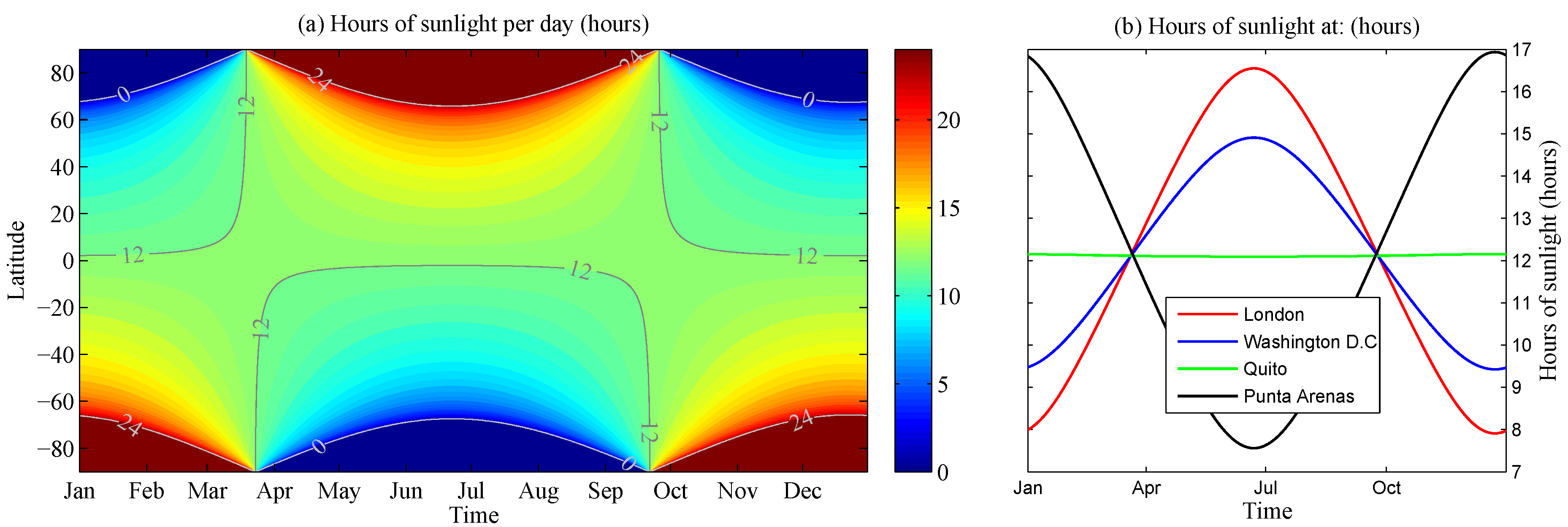
The Nature Run provides the outgoing radiation from Earth in terms of shortwave and longwave radiation. Since DSCOVR constantly views the entire sunlit side of the Earth, all of the calculations and investigations performed in this study are on the daytime half of the Earth. The total outgoing radiation on the sunlit side of the Earth is a function of the amount of incoming radiation, which depends on the location on Earth and the time of year. Figure 1a shows the number of hours of sunlight for all latitudes, calculated with a method described in [6]. Figure 1b shows the number of hours of sunlight per day throughout the year for four cities. The day length is the time duration for which these locations will be visible from the perspective of DSCOVR; hence, for a given sampling rate, the day length determines the number of images that DSCOVR can take over a given region.

Figure 1. (a) Contour plot showing the number of hours of sunlight per day for all latitudes throughout the year; (b) hours of sunlight throughout the year for four cities.

Figure 1. (a) Contour plot showing the number of hours of sunlight per day for all latitudes throughout the year; (b) hours of sunlight throughout the year for four cities.

Studies have shown that over the past decade, the Earth’s energy imbalance has ranged between about 0.5 and 1 Wm${}^{-2}$ [7,8,9]. This level of accuracy is not available from direct satellite measurement at the current time. However, instruments, such as Clouds and the Earth’s Radiant Energy System (CERES), provide reliable enough observations to determine the changes in the net radiation [10,11]. Observations from DSCOVR will also play an important role in tracking energy imbalance. A goal of this work is to analyze whether a particular sampling frequency of the outgoing radiation of the sunlit side of the Earth will provide an accurate measure over shorter, as well as longer time scales.

The analysis can also be used to optimize the observation rate so that an efficient sampling frequency can be chosen without introducing unnecessary error. Analysis of the time series is an important component of satellite product design, as the need for efficiency is balanced with the need for accurate observations and products. Fortunately, DSCOVR has a wide field of view, and the interest is only on the area that it observes. Often, products rely on multiple sensors viewing smaller areas from different satellites with different orbits and sampling rates. This can make the process rather complicated and the errors more significant. For the CERES mission, for example, interpolation techniques have been developed to optimize the sampling of the atmosphere [12]. Some other examples of the complexity involved with optimizing the time stepping are in [13,14]. In the former, a fit function is designed to generate accurate daily means of tropical ice, water and cloudiness. In the latter, a method is presented for estimating the sampling errors in monthly means of the cloud fraction as measured by SEVERI (Spinning-Enhanced Visible and Infrared Imager).

It should be noted that this study only investigates the effect of sampling rate. Other factors, such as instrument calibration, retrieval algorithms, etc., which can also impact the quality of the satellite retrievals, are not considered.

Even though the questions addressed in this study concern the effect of subsampling on DSCOVR-derived information, the results are helpful to satellite remote sensing in general. The remainder of the paper is organized as follows: Section 2 provides a description of the Nature Run dataset and a discussion of the methodology used to analyze the time series. Section 3 shows all of the results for different sampling frequencies and discusses the implications for the instrument. Section 4 provides some concluding remarks.

2. Data and Methodology

In this section, the Nature Run dataset is discussed, and the methodology for analyzing the subsampled time series is introduced.

2.1. The Nature Run

The Nature Run integration begins in May 2005 and runs for just over two years to June 2007. For the purposes of this study, the period from 1 June 2005 to 1 June 2007 is used. The horizontal resolution of the model is approximately 7 km, and 72 model levels up to 0.01 hPa are used. The time step is 5 min, and radiation fluxes are recomputed every 30 min.

The Nature Run was initialized from a realistic atmospheric state and is constrained by realistic boundary conditions throughout the integration. However, since the model runs freely, it diverges from the true atmospheric state within a few days. Nevertheless, validation of the model output has shown the Nature Run to maintain a very realistic atmospheric state throughout the integration [4]. For example, it has tropical storms of an appropriate strength and frequency, approximately correct overall cloud cover and a correctly-varying overall radiation budget.

Figure 2 contrasts the outgoing top-of-atmosphere radiation produced by the Nature Run with that produced by an operational version of GEOS-5. The time shown is 25 September 2006 at 1200 UTC, around 15 months into the Nature Run integration. At this time of the year and day, the Sun is approximately located above the Equator and the Greenwich Meridian. The figure shows the perspective from the L1 Lagrange point. The operational quantities are taken from the beginning of an operational forecast and, so, are effectively the outgoing radiation produced from the data assimilation system. This makes for a field very close to reality, since around 5 million observations are assimilated at each cycle. A comparison between the operational version of GEOS-5 and CERES observations for the top of atmosphere radiation budgets has demonstrated the realism of the system, e.g., [15,16].

Figure 2. Outgoing shortwave radiation for (a) the operational run and (b) the Nature Run; outgoing longwave radiation for (c) the operational run and (d) the Nature Run; outgoing total radiation for (e) the operational run and (f) the Nature Run; all panels are valid at 1200 UTC on 25 September 2006 and from the perspective of the L1 Lagrange point at this time.

Figure 2. Outgoing shortwave radiation for (a) the operational run and (b) the Nature Run; outgoing longwave radiation for (c) the operational run and (d) the Nature Run; outgoing total radiation for (e) the operational run and (f) the Nature Run; all panels are valid at 1200 UTC on 25 September 2006 and from the perspective of the L1 Lagrange point at this time.

It is clear from Figure 2 that the Nature Run produces very realistic looking fields. Although different from reality, the areas of the largest outgoing radiation are located in qualitatively the same locations, and the scale of the structures is similar.

Figure 2a,b shows the outgoing shortwave radiation. Areas of the largest outgoing shortwave radiation are where clouds are located and sunlight is being reflected back into space. This is evident in the tropics, where there are cumulus towers, and in the Southern Hemisphere, where extra-tropical storms propagate around the southern oceans. The relatively high reflectivity of the Saharan and Arabian deserts is evident. A smaller amount of shortwave radiation is reflected by the oceans, due to the low surface albedo. In Figure 2c,d, which shows the outgoing longwave radiation, it is evident that the dominant source is the oceans and the desert. This is due to the higher temperature associated with these regions. In general, clouds reflect more solar radiation than the surface, due to the higher albedo. In contrast, they emit less longwave radiation because of their usually cooler temperatures. Horizontal gradients of outgoing longwave radiation are typically smaller than they are for outgoing shortwave radiation. The range of values for longwave vary by approximately 200 Wm${}^{-2}$, compared to around 850 Wm${}^{-2}$ for shortwave. Albedo can vary significantly at relatively short horizontal scales, resulting in larger differences in outgoing shortwave radiation across small distances.

The focus of this study is on capturing temporal variations of the Earth’s radiation budget over the sunlit hemisphere. It would be useful to compare the temporal variations of this measure in the Nature Run with those from observations. This can be problematic, since a specific location can have quite sparse temporal resolution, and gap filling typically involves error introducing interpolation [12]. Instead of comparing to observations directly, the Nature Run temporal evolution is again compared to the GEOS-5 operational system. Outgoing radiation is given every 30 min, and forecasts are a maximum of 6 h, the interval at which data assimilation is performed.

Figure 3 compares the time series of outgoing shortwave and longwave radiation from the Nature Run and the operational system for the month of September 2006. Each data point in the time series in the figure is calculated by spatially averaging the outgoing radiation across the sunlit side of Earth. Data are output on a latitude-longitude grid, so a cosine of latitude area weighting is applied in the spatial averaging. A particular grid point is considered sunlit when the incoming sunlight covers more than half of the grid area. The figure demonstrates that the typical diurnal cycle is captured well by the Nature Run. For outgoing longwave radiation, the amplitude and frequency is very similar to reality, even though the atmospheric state is different. For outgoing shortwave radiation, the structure of the time series has larger differences, due to the dependency on clouds and specific weather, which will be different in the Nature Run. The average outgoing shortwave radiation in the Nature Run for this period is slightly higher due to slightly more cloud cover. Despite the differences, however, it is clear that the kinds of scales seen for the realistic system are seen in the Nature Run and that they behave similarly.

Figure 3. Comparison of longwave and shortwave outgoing radiation for the Nature Run and operational GEOS-5. The time series shows the month of September 2006.

Figure 3. Comparison of longwave and shortwave outgoing radiation for the Nature Run and operational GEOS-5. The time series shows the month of September 2006.

For the Nature Run to be useful for simulating DSCOVR observations requires it to have realistic spatial and temporal scales in the outgoing radiation fields. The comparison with the operational system, which is very close to reality, shows this to be the case for the scales captured by that system.

Figure 4 shows the time series of outgoing longwave and shortwave radiation across the entire Nature Run period. Similar to Figure 2, Figure 4 demonstrates that the shortwave radiation has larger variation compared to the longwave. When averaged over the sunlit half of the Earth, longwave radiation is larger than its shortwave counterpart. Slight peaks occur in outgoing longwave in the late Northern Hemisphere summer, due to the greater land mass of the Northern Hemisphere being orientated slightly more towards the Sun. The outgoing shortwave radiation has a much larger amplitude in both the annual and daily cycles. The peak of the annual cycle occurs in the Southern Hemisphere summer. This is due to the relatively large and highly reflective surface of Antarctica coming into view of the Sun, as well as cloud tops of the Southern Hemisphere storm track. The greater daily variations in the outgoing shortwave radiation are in part due to the contrast between land and ocean. Generally, when the sunlit side of the Earth is the Pacific Ocean, outgoing shortwave radiation will be less than when a large landmass dominates the sunlit side.

Figure 4. Time series of outgoing longwave and shortwave radiation produced by the GEOS-5 Nature Run. The time series covers a two-year period from 1 June 2005 to 1 June 2007.

Figure 4. Time series of outgoing longwave and shortwave radiation produced by the GEOS-5 Nature Run. The time series covers a two-year period from 1 June 2005 to 1 June 2007.

2.2. Methodology

The original Nature Run time series provides a suitable substitute of the truth, and a subsampling of the time series with a specific frequency mimics the observations of DSCOVR, or some other satellite. Here, observations from DSCOVR are simulated by taking the outgoing radiation on the sunlit side of the Earth, as shown in Figure 4.

The Nature Run outputs the radiation fields every 30 min; let t be the original truth time series of the outgoing radiation (shortwave, longwave or total) from the sunlit side of the Earth, then:

$$t=\left\{t_1,t_2,\dots \right\}$$

(1)

where subscripts denote output times.

For a particular sampling frequency, a subsample can be constructed by choosing a specific starting point. There are $2n$ potential starting points, where n is sampling frequency in hours; hence, $2n$ time series can be constructed for a sampling frequency of every n hours. Let $r_{n,j}$ be the subsample time series corresponding to the j-th starting point, where $j=1,\dots ,2n$, then:

$$r_{n,j}=\left\{r_{n,j,1},r_{n,j,2},\dots \right\}$$

(2)

To further clarify how the subsampled time series are constructed, Figure 5a shows examples with the total outgoing radiation time series, for the time period 20 June 2006 at 0000 UTC to 23 June 2006 at 0000 UTC. The different curves show the original Nature Run time series and subsamples obtained for this period with different sampling frequencies, but the same starting point. The effect of the subsampling can be clearly seen from Figure 5a. As the sampling frequency becomes coarser and coarser, more and more details of the original time series are lost. To quantify the effect of the subsampling, a suite of of metrics is adopted. These metrics, which are described in detail in the following sections, include the uncertainties in the mean, the absolute error in the subsamples, the correlation between the subsamples and the original time series and normalized errors.

The original Nature Run time series in Figure 5a also serves to demonstrate how the outgoing radiation can vary on daily time scales. At this time of year, there is generally a sudden increase in outgoing radiation with a peak at around 0600 to 0900 UTC. After the peak occurs, outgoing radiation tails off to a daily low at around 0000 UTC. The lowest values generally coincide with the Sun being over the Pacific Ocean. The sudden increase is then due to the large land masses of Asia coming into view. The peak values occur when mostly land is in view of the Sun, and the tail-off occurs as the Atlantic Ocean comes into view. Smaller local maximums occur due to the North American continent. Differences from day to day result from different weather patterns and cloud locations.

Figure 5. (a) Nature Run time series of total outgoing radiation for a three-day period in June 2006. Colored curves show single realizations from the various sampling intervals for the same period; (b) The daily means for just 20 June 2006 for all of the realizations from the various sampling intervals.

Figure 5. (a) Nature Run time series of total outgoing radiation for a three-day period in June 2006. Colored curves show single realizations from the various sampling intervals for the same period; (b) The daily means for just 20 June 2006 for all of the realizations from the various sampling intervals.

2.2.1. Uncertainties in the Mean

The daily, monthly, seasonal and annual means of outgoing radiation are critical parameters in climate studies. As mentioned above, for each given subsampling frequency, multiple time series can be constructed. Different subsamples will give different means; the variability of these means can be used as the metric to show the uncertainty in subsampling. Figure 5b gives an example of this metric. Here, the daily means $\overline{r_{n,j}}$, for every sampling frequency and starting point, are plotted against sample frequency. The interval for which means are calculated is 20 June 2006 at 0000 UTC to 21 June 2006 at 0000 UTC. When the sampling frequency is between 1 and 4 h, the daily mean spread is quite small. When the sampling frequency is 24 h only, one location is effectively sampled each day, and the spread is large.

To generalize for a specific interval, be it a day, a month, a season or a year, the uncertainty of the mean can be measured with the standard deviation of the difference between full and subsampled time series over all possible subsamples. Let $\overline{r_{n,j}}$ be the interval mean for the j-th subsample and $\overline{t}$ be the mean of the original time series (“the truth”). Note $\overline{r_{n,j}}$ and $\overline{t}$ are also time series, but with each point in the series being for each interval. The standard deviation of the difference between full and subsampled time series interval means can be calculated as,

$${\sigma }_{r,n}=\sqrt{\frac{1}{2n}{\displaystyle \sum _{j=1}^{2n}}{\overline{r_{n,j}}}^2-{\left(\frac{1}{2n}{\displaystyle \sum _{j=1}^{2n}}\overline{r_{n,j}}\right)}^2}$$

(3)

Note that $\overline{r_{n,j}}$ is a subsample of t, so when averaged over different starting points j, it is just an average of the entire truth time series. Therefore, Equation (3) reduces to,

$${\sigma }_{r,n}=\sqrt{\frac{1}{2n}{\displaystyle \sum _{j=1}^{2n}}{\overline{r_{n,j}}}^2-{\overline{t}}^2}$$

(4)

The average standard deviation of the difference between full and subsampled time series over the entire Nature Run time period provides a measure of the overall uncertainty:

$$\overline{{\sigma }_{r,n}}=\frac{1}{m}\sum _{k=1}^m{\left[{\sigma }_{r,n}\right]}_k$$

(5)

where m is the number of possible intervals. For the Nature Run period, there are 720 days, 24 months, 8 seasons or 2 years, so $m=720$ if considering daily means.

2.2.2. Absolute Error in the Mean

Instead of computing the daily, monthly, seasonal and annual means, the error compared to the true mean for that interval can be used. For a given sampling frequency of every n hours, the absolute error time series can be written as:

$${\delta }_{r,n}=\frac{1}{2n}\sum _{j=1}^{2n}\left|\overline{r_{n,j}}-\overline{t}\right|$$

(6)

The average absolute error over the entire Nature Run for a given sampling frequency is,

$$\overline{{\delta }_{r,n}}=\frac{1}{m}\sum _{k=1}^m{\left[{\delta }_{r,n}\right]}_k$$

(7)

where m is the number of possible intervals. For example, $m=24$ if considering monthly means.

2.2.3. Correlation

One drawback of examining the data only with the interval mean is that it does little to compare the structure of the time series. It is likely that peaks and sudden changes in the time series are aliased, and the computation of the mean does not always provide a measure of this. Indeed, the error in the mean could be zero, even when large aliasing occurs.

A challenge with the comparison of the original and subsampled time series being made here is that the data are sampled at different rates, and the time series is generally not periodic. This prevents the use of techniques that could be useful, such as looking at Fourier coefficients and comparing a power spectrum. One way that the structure of the original and subsampled time series can be compared though is by measuring the correlation coefficient between them. Computing the correlation coefficient between two time series provides a quantitative sense of how similar the two series are. If a particular subsampled time series accurately represented the interval mean by chance, without having very similar overall structure, it would be revealed by a low correlation coefficient.

Since the sampling frequency is different, each subsampled time series is linearly interpolated back to the same sample locations as the original time series to facilitate computing correlation coefficients. The correlation coefficient:

$$R_{n,j}=\mathrm{corr}\left(p_{n,j},t\right)$$

(8)

where $p_{n,j}$ is the linearly-interpolated time series, is computed for each possible starting point. As above, a mean value is computed across all starting points within a particular frequency, denoted $\overline{R_n}$. In addition to that, the standard deviation of the correlation coefficients across all starting points is computed, ${\sigma }_{R,n}$.

2.2.4. Error Norms

Using the linearly-interpolated time series, it is also possible to compute normalized errors. The error is computed at all original sample points using three normalized measures,

$$l_1=\frac{1}{N}\sum _{i=1}^N\left|{ϵ}_i\right|,l_2={\left(\frac{1}{N}\sum _{i=1}^N{\left|{ϵ}_i\right|}^2\right)}^{\frac{1}{2}}\mathrm{and}{l}_{\infty }=max\left(|{ϵ}_i|\right)$$

(9)

where ϵ is the difference between the linearly-interpolated subsampled time series and the original Nature Run time series and N is the number of samples in the interval.

Like for the correlation coefficients, measuring the error in these ways provides insight into the amount of aliasing that occurs and how much error could be present at any given instant, on average. The $l_1$ measures the average difference between the subsampled time series and the truth at all locations; hence, the $l_1$ error can be large, even if the error in the mean is not.

3. Results

In this section, the time series of outgoing radiation produced by the Nature Run is subsampled and analyzed with the above metrics.

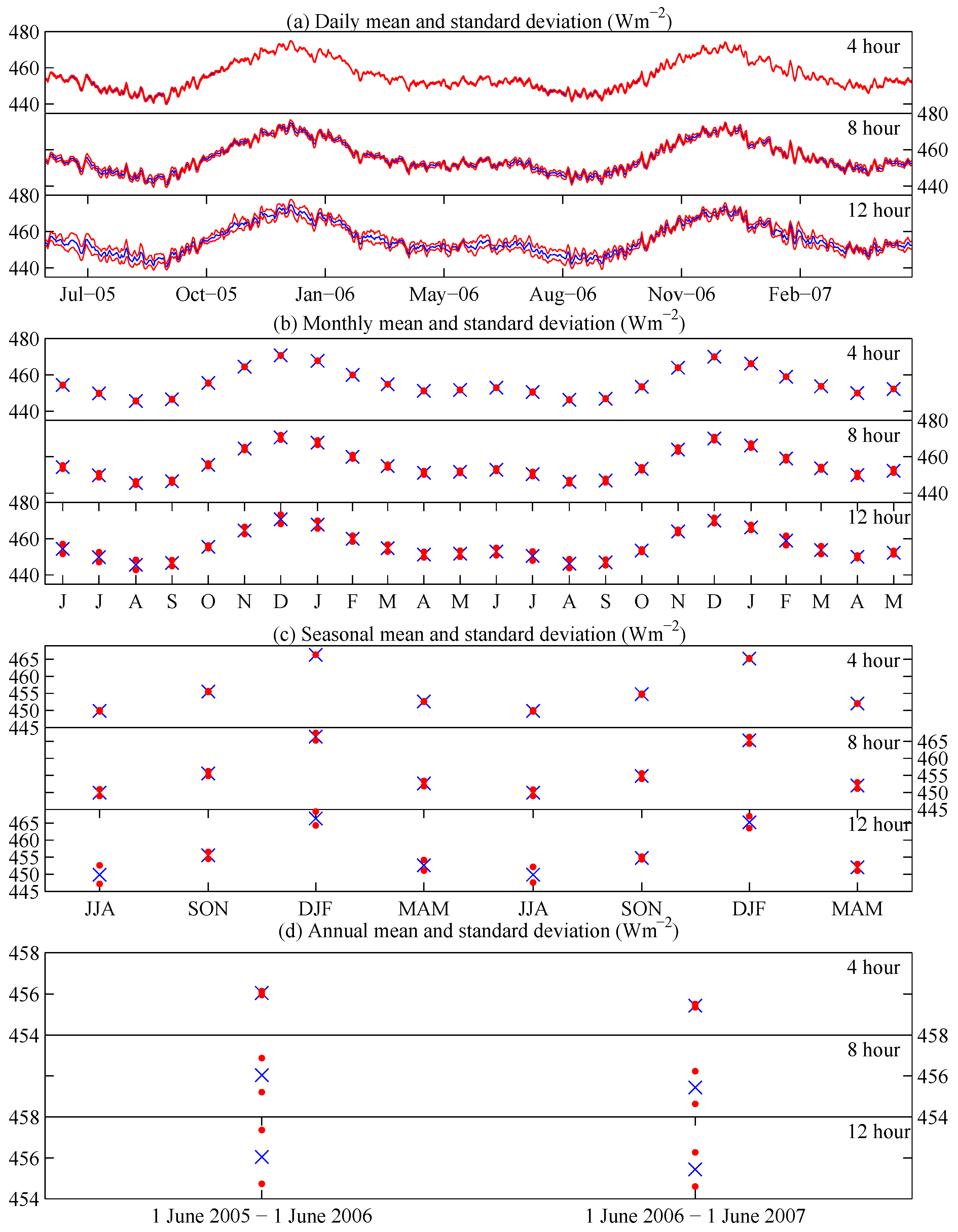
Figure 6a shows the daily mean $\overline{t}$ and mean plus and minus one standard deviation of the difference between full and subsampled time series $\overline{t}\pm {\sigma }_{r,n}$ for the 720 days of the Nature Run. The figure shows the results for the total outgoing radiation, i.e., the sum of the shortwave and longwave. The three panels show the results for the $n=$ 4-, 8- and 12-h sampling frequency; other sampling frequencies are omitted from these plots. Figure 6b shows the monthly mean and standard deviation of the difference between full and subsampled time series; Figure 6c shows the seasonal values; and Figure 6d shows the annual values. Note that vertical scaling is kept fixed within each of the three sub-panels, but is not fixed for the entire figure.

Figure 6. The blue curves/points show $\overline{t}$ for the (a) daily; (b) monthly; (c) seasonal and (d) annual intervals. The red curves/points show $\overline{t}\pm {\sigma }_{r,n}$. Within each panel, the three sub-panels show, from top to bottom, a 4-, 8- and 12-h sampling frequency. The vertical scale is fixed within each set of three panels.

Figure 6. The blue curves/points show $\overline{t}$ for the (a) daily; (b) monthly; (c) seasonal and (d) annual intervals. The red curves/points show $\overline{t}\pm {\sigma }_{r,n}$. Within each panel, the three sub-panels show, from top to bottom, a 4-, 8- and 12-h sampling frequency. The vertical scale is fixed within each set of three panels.

The results in Figure 6 show that when a 4-h sampling is used, the standard deviation of the difference between full and subsampled time series is relatively small compared to overall variations of the mean across all time scales. For the daily mean, the standard deviations do not exceed 1.19 Wm${}^{-2}$; given that daily means are of the order of 450 Wm${}^{-2}$ and vary by around 5 Wm${}^{-2}$ in a day, this would likely be a reasonable variation to encounter in observations. As expected, for 8- and 12-h sampling frequencies, the uncertainty increases. In the daily means, the spread is much more evident, and even for the long time scale annual mean, there is significantly more spread with an 8-h sampling frequency than with 4 h.

The interval means are largest in and around December, as seen in Figure 4. The spread for daily means appears fairly consistent throughout the year. From the monthly and seasonal means, it can be seen that the time of year with the least spread is around October and April. The standard deviation of the difference between full and subsampled time series on the monthly and seasonal means of this period is smallest and is similar for both occurrences of these periods in the Nature Run. The two annual means are similar, 456.04 Wm${}^{-2}$ and 455.43 Wm${}^{-2}$. The annual mean spread is around ten-times larger when the sampling frequency is halved from every 4 h to every 8 h.

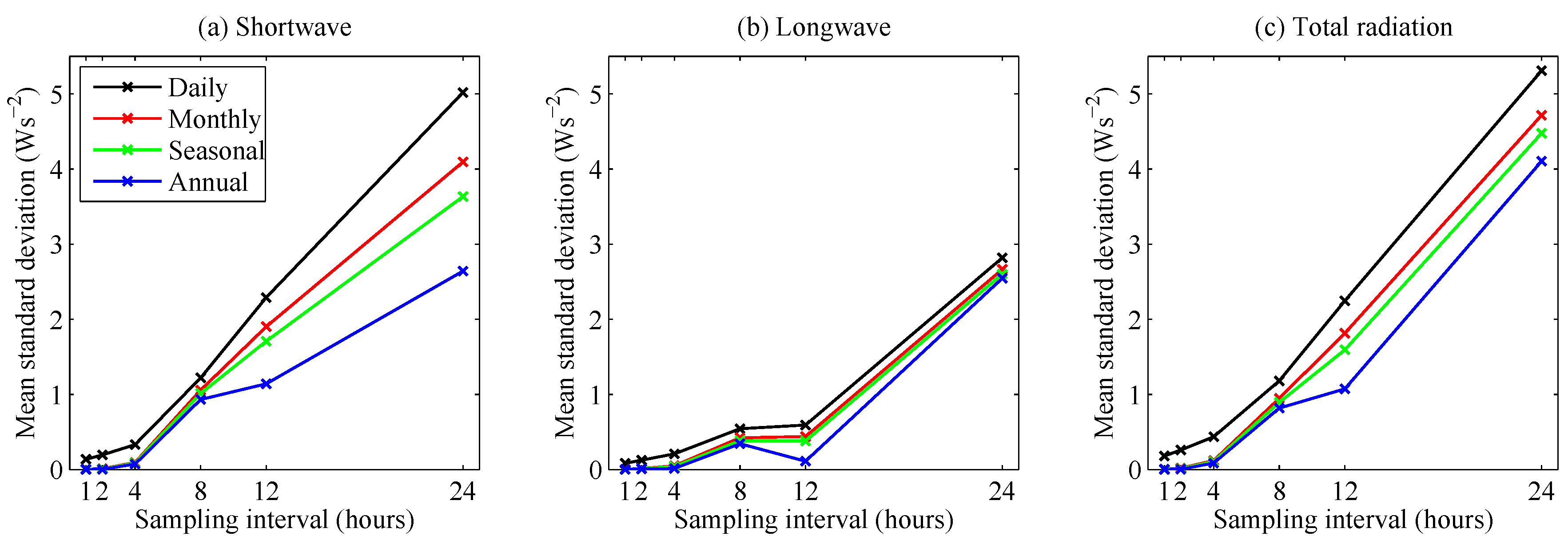
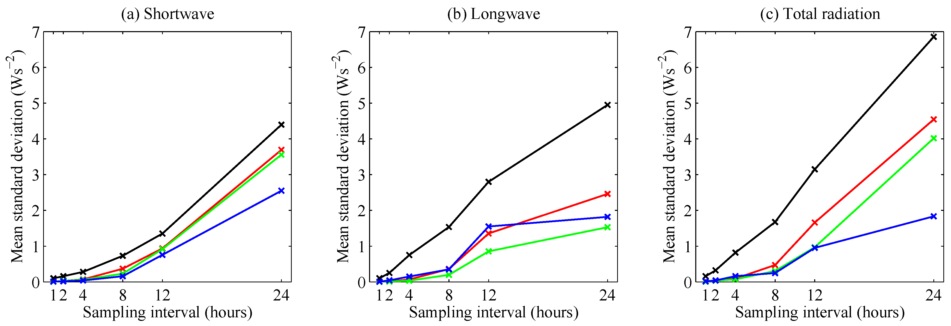
The findings are generalized by computing $\overline{{\sigma }_{r,n}}$ for shortwave, longwave and total radiation separately; these results are shown in Figure 7. Each curve shows the average standard deviation of the difference between full and subsampled time series, i.e., a data point in Figure 7 corresponds to the mean of the standard deviations represented by an entire red curve or set of red points in Figure 6. Note that more sample frequencies are shown in Figure 7 than in Figure 6. Standard deviations of the difference between full and subsampled time series are larger for shortwave radiation than for longwave radiation, due to the smaller spatial and temporal scales associated with shortwave radiation. The magnitudes of the standard deviations of the difference between full and subsampled time series for the total radiation are dominated by the shortwave. These results suggest a reduced frequency would likely be acceptable if only longwave radiation were of interest.

Figure 7. The mean of the standard deviations of the difference between full and subsampled time series $\overline{{\sigma }_{r,n}}$ for (a) shortwave; (b) longwave and (c) total radiation.

Figure 7. The mean of the standard deviations of the difference between full and subsampled time series $\overline{{\sigma }_{r,n}}$ for (a) shortwave; (b) longwave and (c) total radiation.

As anticipated, the uncertainty increases as the sample interval does. For a sampling interval of 1 h, the standard deviation of the difference between full and subsampled time series is negligible for all but the daily means. There are two general regimes when computing the daily mean, a sampling frequency of 4 h and above and below four hours. For example when decreasing the frequency from 1 h to 2 h or 2 h to 4 h, the standard deviation of the difference between full and subsampled time series increases by around 63% for shortwave radiation. Conversely, when decreasing frequency from 4 h to 8 h, the standard deviation of the difference between full and subsampled time series increases by 430% for shortwave radiation. Between 8 h and 12h and 24 h, a similar rate of increase in average standard deviation is seen. For longwave radiation, the increase in average standard deviation of the difference between full and subsampled time series is more gradual between 1 and 12 h and changes little between 8 and 12 h. Sampling the Earth every 12 h results in only one observation per day for any given location. It should be noted that the standard deviation of the annual mean for the 8-h subsample is comparable to the Earth’s energy imbalance [7,8,9]; hence, a sample frequency of every 8 h or coarser is not suitable for radiation budget studies.

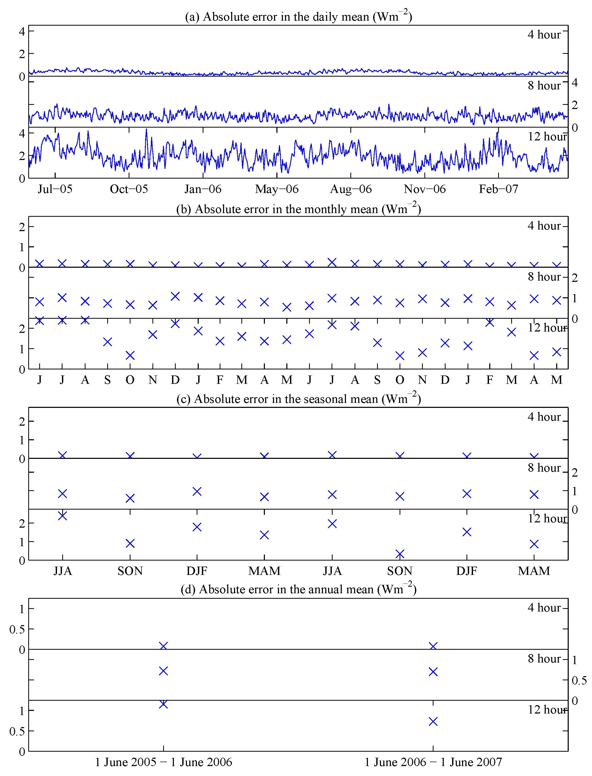
Figure 8. As for Figure 6, (a) daily; (b) monthly; (c) seasonal and (d) annual intervals, but showing just ${\delta }_{r,n}$.

Figure 8. As for Figure 6, (a) daily; (b) monthly; (c) seasonal and (d) annual intervals, but showing just ${\delta }_{r,n}$.

Figure 8, constructed like Figure 6, shows the absolute errors in the interval mean, ${\delta }_{r,n}$. When using a sampling frequency of 4 h, the absolute errors in the interval mean are relatively small, generally between 0.1 Wm${}^{-2}$ and 0.5 Wm${}^{-2}$ for the daily mean and even smaller for the monthly, seasonal and annual intervals. For the 8-h sampling frequency, the errors for the daily interval increase to between 1 Wm${}^{-2}$ and 2 Wm${}^{-2}$, and for the monthly, seasonal and annual intervals are around 1 Wm${}^{-2}$. When using the 12-h sampling frequency, absolute errors for the daily interval can be larger than 4 Wm${}^{-2}$. For monthly, seasonal and annual intervals, the errors range from 1 Wm${}^{-2}$ to 2 Wm${}^{-2}$, but have much more variation between periods than for 4- and 8-h frequencies. Examining the standard deviation of the difference between full and subsampled time series in Figure 6, it is difficult to determine if there are annual variations in spread. As is evident comparing sampling frequencies of 8 and 12 h in Panels (b), (c) and (d) between Figure 8 and Figure 6, the largest spread occurs when the absolute errors are also large. Therefore, looking at the absolute error helps reveal any annual cycles that occur in both errors and spread. For the absolute errors in the daily mean, there are slightly larger errors in the summer months when using a 4-h sample frequency. For the lower frequency sampling, no annual signal is evident for the daily interval. For absolute errors in the monthly mean, there is a slight summer increase for the 4-h sampling frequency. For 8 and 12 h, it is harder to determine if any significant cycle occurs, though errors do seem slightly smaller in the autumn months. For the seasonal and annual intervals, there are insufficient samples to determine any pattern.

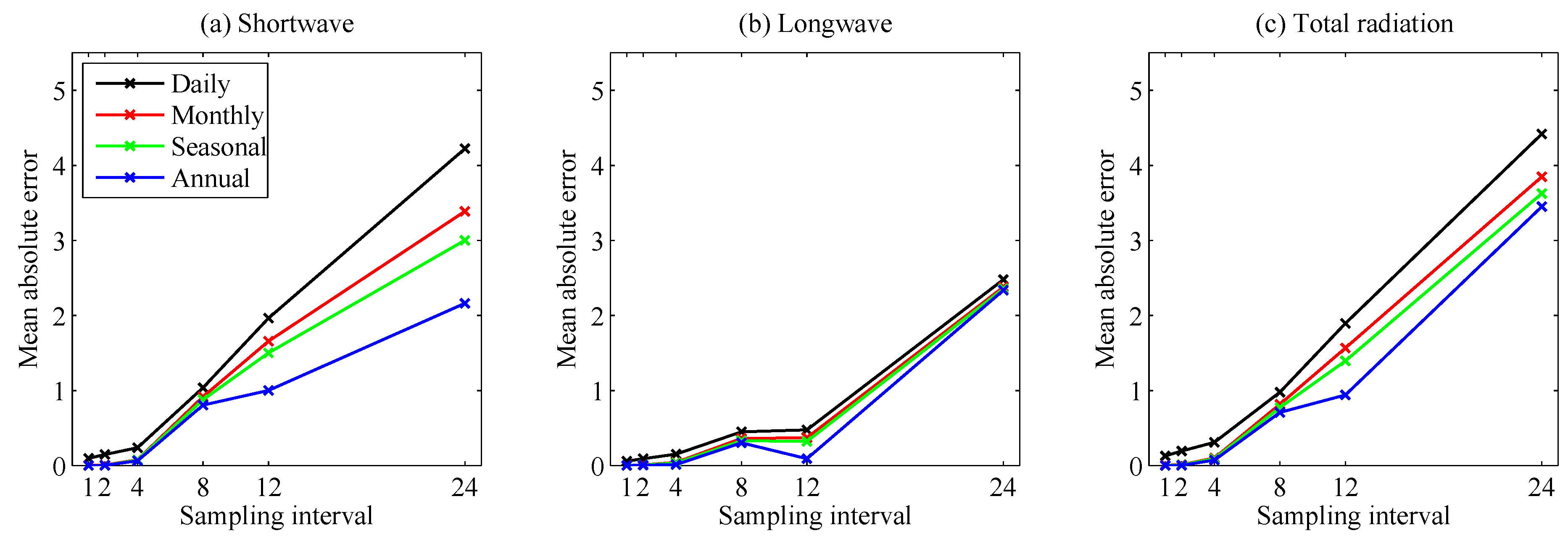
As above, the results are generalized by taking the average over all intervals to give $\overline{{\delta }_{r,n}}$, shown in Figure 9. By definition, the mean standard deviation of the difference between full and subsampled time series and the mean absolute error are correlated; hence, the results in Figure 9 have the same characteristics as were shown in Figure 7. However, since they are showing the properties of subsamples from different perspectives, both are provided. Again, the overall findings are that errors start to increase more rapidly once the sampling frequency is reduced below 4 h. The effect is more dramatic for the shortwave radiation, where spatial and temporal variations are larger than for longwave radiation.

Figure 9. As for Figure 7, (a) shortwave; (b) longwave and (c) total radiation, but showing $\overline{{\delta }_{r,n}}$.

Figure 9. As for Figure 7, (a) shortwave; (b) longwave and (c) total radiation, but showing $\overline{{\delta }_{r,n}}$.

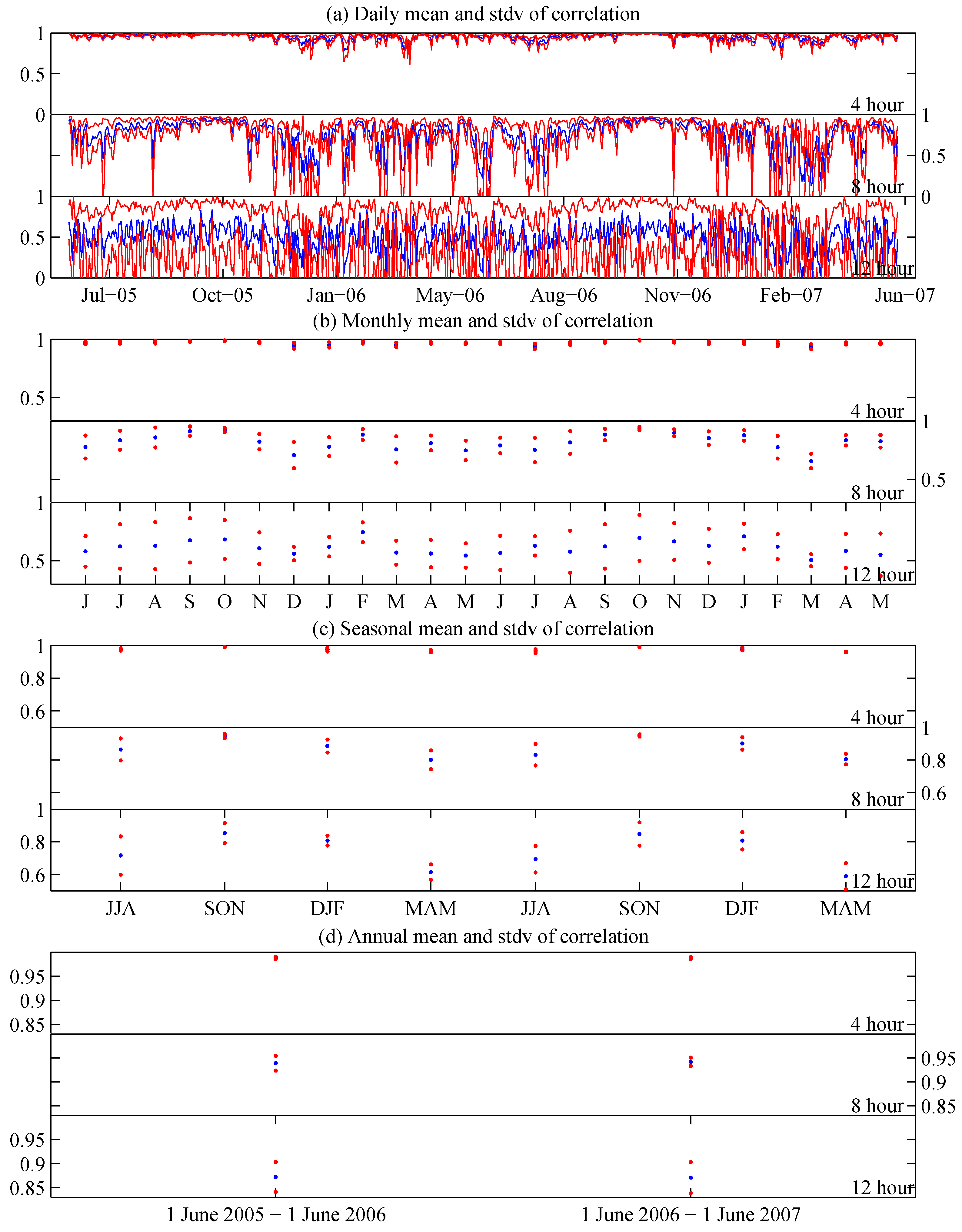
Figure 10 shows mean correlation $\overline{R_n}$ and correlation spread $\overline{R_n}\pm {\sigma }_{R,n}$ for the daily, monthly, seasonal and annual intervals. The data are displayed as in Figure 6 and Figure 8. For the 4-h sampling frequency, the correlations are generally close to one, and the standard deviations of the correlation coefficient are small for most of the intervals. Some decreases in mean correlations for this sampling frequency are seen in the Northern Hemisphere winter time. For 8- and 12-h sampling frequencies, the correlations get significantly smaller for the daily interval. For a 4-h sampling frequency, the monthly, seasonal and annual correlation coefficients are all close to one, and the standard deviations are small, showing that the structure of the time series is very similar for all starting points. For monthly intervals, the correlations remain high for the 8-h sampling frequency, but can reduce below 0.5 for the 12-h sample frequency. Seasonal and annual correlations are close to one, and the standard deviations of the correlation coefficients are small for all sample frequencies.

Table 1 shows the means and standard deviations of the $l_1$, $l_2$ and $l_{\infty }$ normalized errors for the daily interval. Values are computed by generating subsampled time series for each day and then interpolating those time series. Error norms are computed for every start point, and mean and standard deviation over all starting points for a given frequency are computed.

The $l_1$ and $l_2$ errors measure the differences between a subsample and the original truth time series; $l_{\infty }$ gives the maximum difference, focusing on where the aliasing is most significant. Examining the subsampled time series in this metric gives slightly different results than seen for the interval means. Here, the errors increase most rapidly for the highest frequency sampling rates, for example the standard deviation of $l_{\infty }$ with the 2-h frequency is around 60-times larger than with the 1-h frequency. Effectively, the measures demonstrate that errors at a specific time due to aliasing increase fairly consistently. Unlike in computing the means, there is not a more rapid increase in these metrics when below a certain sampling frequency.

Figure 10. As for Figure 6, (a) daily; (b) monthly; (c) seasonal and (d) annual intervals, but showing $\overline{R_n}$ and $\overline{R_n}\pm {\sigma }_{R,n}$.

Figure 10. As for Figure 6, (a) daily; (b) monthly; (c) seasonal and (d) annual intervals, but showing $\overline{R_n}$ and $\overline{R_n}\pm {\sigma }_{R,n}$.

Table 1. Means and standard deviations of the normalized errors for the daily interval.

	${\mathit{l}}_{\mathbf{1}}$ Error (Wm${}^{\mathbf{-}\mathbf{2}}$)		${\mathit{l}}_{\mathbf{2}}$ Error (Wm${}^{\mathbf{-}\mathbf{2}}$)		${\mathit{l}}_{\mathbf{\infty }}$ Error (Wm${}^{\mathbf{-}\mathbf{2}}$)
Sampling freq.	Mean	SD	Mean	SD	Mean	SD
1 h	0.1040	0.0029	0.1834	0.0024	0.5958	0.0010
2 h	0.3842	0.0123	0.5557	0.0164	1.5579	0.0594
4 h	1.0934	0.0965	1.4912	0.1358	3.7740	0.3610
8 h	2.4855	0.2277	3.2808	0.3161	7.4871	0.8056
12 h	3.6515	0.3420	4.7048	0.5102	9.9982	1.3570

Table 1. Means and standard deviations of the normalized errors for the daily interval.

	${\mathit{l}}_{\mathbf{1}}$ Error (Wm${}^{\mathbf{-}\mathbf{2}}$)		${\mathit{l}}_{\mathbf{2}}$ Error (Wm${}^{\mathbf{-}\mathbf{2}}$)		${\mathit{l}}_{\mathbf{\infty }}$ Error (Wm${}^{\mathbf{-}\mathbf{2}}$)
Sampling freq.	Mean	SD	Mean	SD	Mean	SD
1 h	0.1040	0.0029	0.1834	0.0024	0.5958	0.0010
2 h	0.3842	0.0123	0.5557	0.0164	1.5579	0.0594
4 h	1.0934	0.0965	1.4912	0.1358	3.7740	0.3610
8 h	2.4855	0.2277	3.2808	0.3161	7.4871	0.8056
12 h	3.6515	0.3420	4.7048	0.5102	9.9982	1.3570

Arctic Region

The results presented above are computed for the entire sunlit side of the Earth. Now, the area is reduced to only consider the Arctic, a region that has been experiencing an unprecedented change for the past few decades [17]. The radiation budget over the Arctic is one of the main factors that drives these changes [18]. DSCOVR presents a valuable opportunity to study polar regions, especially during the polar summer, when the region is orientated towards the Sun. This is an area with otherwise fairly sparse observation coverage. Indeed, a satellite located at the L2 Lagrange point has been proposed, so that the polar winter could be continuously observed, too, and satellite coverage of the entire Earth simultaneously could be achieved [19].

At some points during the year, the Arctic region (north of 66${}^{\circ }$N) will be orientated away from the Sun (polar night) and, so, not visible to DSCOVR. As such, the time series of outgoing radiation in this region, as seen from the L1 Lagrange point, is not continuous. In the statistical metrics used here, the days, months and seasons for which at least part of the interval is not sunlit are neglected. For the annual metrics, this is not possible, so instead, all of the times when a measurement is made are initially included.

Figure 11 shows the same metrics shown in Figure 7, but here for the Arctic region. The standard deviations of the difference between full and subsampled daily means are larger for the total radiation in the Arctic sunlit region than they are for the global sunlit region. However, the larger contribution now comes from the longwave radiation, rather than shortwave radiation. For Earth as a whole, the average weather, and therefore cloud cover, is quite constant, whereas when focusing on a small region like the Arctic, the average conditions can be more varied, giving rise to larger fluctuations in outgoing longwave radiation. Near the beginning and end of the polar night, there is significant daily variation in the outgoing total radiation. At this time, only a very small sliver is being observed, and weather or the type of land in view in that region can be highly varied over the course of a day.

Figure 11. As for Figure 7, (a) shortwave; (b) longwave and (c) total radiation, but for the Arctic region.

Figure 11. As for Figure 7, (a) shortwave; (b) longwave and (c) total radiation, but for the Arctic region.

It is interesting to note that when sampling at 4 h and examining longwave or total radiation, the average standard deviation of the difference between full and subsampled time series is actually larger than for the monthly and seasonal intervals. This is due to the method used in the data processing. Since monthly and seasonal means are only computed when at least some sunlight is present for the entire interval, the regions closest to where the polar night begins and ends are not included. However, the annual mean is computed using data right up to where Arctic polar night begins and ends, and so, the higher variation that is seen in longwave radiation at this time is included. When a few weeks of data for either side of the polar night are arbitrarily omitted from the annual mean calculation, the average standard deviation of the difference between full and subsampled time series is smaller than for monthly and seasonal means. This is also the case for the 8- and 12-h sampling frequency when examining longwave radiation. The characteristics of the absolute error in the interval mean for the Arctic region are very similar to those of the average standard deviations of the difference between full and subsampled time series (not shown), as seen globally.

4. Conclusions

A two-year time series of outgoing radiation, as produced by the high resolution Goddard Earth Observing System Version-5 (GEOS-5) Nature Run, has been analyzed. The objective of this work has been to assess the impact of temporal sampling frequency on DSCOVR-retrieved radiation budget. The findings of this study can thus also inform the optimization of the temporal sampling that will be used with observations. The Nature Run data were chosen for their high temporal and spatial resolution, because these offer a consistent model run over a long period and because they do not suffer from discrete re-initialization steps due to data assimilation.

Potential sampling frequencies ranging from 1 h to 24 h were examined in the study. Simulation of the observations was achieved by subsampling the full Nature Run time series of outgoing (top-of-atmosphere) radiation. Experiments were performed treating longwave and shortwave radiation separately and for total radiation.

The ability of different sampling rates to capture the time series of outgoing radiation was first analyzed in the context of daily, monthly, seasonal and annual means. For each sampling frequency, there are a number of possible starting points. Computing the interval mean for all of the possible starting points for a particular sampling frequency and then computing the standard deviation of those means gives an insight into the variability. Results show that higher sampling frequency definitely gives more information and less uncertainty. Sampling frequency coarser than every 4 h results in significant error.

The absolute error in the interval means were also compared, where interval means for each sampling frequency and starting point were compared directly to the true interval mean. This metric provides further insight into the behavior of a given sampling, particularly by revealing seasonal cycles. Averages of the standard deviation of the difference between full and subsampled time series, as well as absolute errors were taken over all possible intervals. Differences between longwave and shortwave radiation were compared in this setting; it was shown that errors and spread in sampling shortwave radiation grow more rapidly than for longwave radiation. This is due to the more variable nature of shortwave radiation over the intervals being examined.

In order to assess the similarity between the structure of the sampled time series and the full time series, correlation coefficients between the two were considered. The mean and standard deviations of the correlation coefficients with daily, monthly, seasonal and annual intervals across all starting points were computed. This provides a measure of how much the similarity between the two time series varies with different sampling rates. A sampling rate of around 4 h was shown to perform well for monthly, season and annual intervals. For the 4-h sampling rate, correlations of 0.9 or more are often seen for the daily interval, almost always for monthly intervals and always for seasonal and annual intervals.

In the final part of this work, the experiments were repeated, but only considering the Arctic region. Here, the variations were found to be larger, increasing the uncertainly for each sampling frequency. Around the time the Arctic polar night begins and ends, the uncertainty becomes particularly large. If this region, or the Antarctic region, were being examined in detail, it would likely be necessary to increase the sampling frequency. There is more uncertainty in sampling longwave radiation in the Arctic than shortwave radiation, unlike for the rest of the sunlit region of the Earth, where the opposite was found to be true.

We note that a higher DSCOVR sampling frequency is definitely helpful and sometimes a must for conducting some of the studies, such as atmosphere correction and vegetation indices retrieval. This paper only focuses on radiation budget. In Part 2 of this work, the cloud cover is examined. In order to produce the full outgoing radiation product from DSCOVR, it will be necessary to also formulate information about the spatial structure of the atmosphere. Analyzing the time series of cloud cover will further inform the temporal sampling required.