Article

Rank-Based Methods for Selection of Landscape Metrics for Land Cover Pattern Change Detection

1
Soil and Agronomy, School of Environmental and Rural Science, University of New England, Armidale, NSW 2351, Australia
2
Ecosystem Management, School of Environmental and Rural Science, University of New England, Armidale, NSW 2351, Australia
*
Author to whom correspondence should be addressed.
These authors contributed equally to this work.
Remote Sens. 2016, 8(2), 107; https://doi.org/10.3390/rs8020107
Submission received: 12 November 2015 / Revised: 10 January 2016 / Accepted: 20 January 2016 / Published: 1 February 2016

Abstract

:
Often landscape metrics are not thoroughly evaluated with respect to remote sensing data characteristics, such as their behavior in relation to variation in spatial and temporal resolution, number of land cover classes or dominant land cover categories. In such circumstances, it may be difficult to ascertain whether a change in a metric is due to landscape pattern change or due to the inherent variability in multi-temporal data. This study builds on this important consideration and proposes a rank-based metric selection process through computation of four difference-based indices (β, γ, ξ and θ) using a Max–Min/Max normalization approach. Land cover classification was carried out for two contrasting provinces, the Liverpool Range (LR) and Liverpool Plains (LP), of the Brigalow Belt South Bioregion (BBSB) of NSW, Australia. Landsat images, Multi Spectral Scanner (MSS) of 1972–1973 and TM of 1987–1988, 1993–1994, 1999–2000 and 2009–2010 were classified using object-based image analysis methods. A total of 30 landscape metrics were computed and their sensitivities towards variation in spatial and temporal resolutions, number of land cover classes and dominant land cover categories were evaluated by computing a score based on Max–Min/Max normalization. The landscape metrics selected on the basis of the proposed methods (Diversity index (MSIDI), Area weighted mean patch fractal dimension (SHAPE_AM), Mean core area (CORE_MN), Total edge (TE), No. of patches (NP), Contagion index (CONTAG), Mean nearest neighbor index (ENN_MN) and Mean patch fractal dimension (FRAC_MN)) were successful and effective in identifying changes over five different change periods. Major changes in land cover pattern after 1993 were observed, and though the trends were similar in both cases, the LP region became more fragmented than the LR. The proposed method was straightforward to apply, and can deal with multiple metrics when selection of an appropriate set can become difficult.

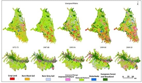
Graphical Abstract

1. Introduction

Numerous landscape metrics have been developed from cover class maps generated from remote sensing data to better understand the spatial arrangements between different cover classes, particularly forest fragments [1]. These spatial arrangements are expressed numerically in the form of landscape indices or pattern metrics offering great potential for understanding the links among ecological pattern, function, and processes, and monitoring of landscape pattern, transition, and change [2,3,4] or as variables for models supporting environmental assessment and planning efforts (e.g., [5,6,7,8,9]). However, improper landscape metric selection and conceptual flaws in landscape pattern analysis have sometimes been problematic [10]. For example, the statistical properties, limitations and behavior of metrics across a range of values and landscapes, and the sensitivity of metrics to changing landscape patterns are still not fully understood [11,12].
Pattern metrics can be computed using freeware such as FRAGSTAT [13], Patch Metrics [14] and others [15,16,17]. However, many metrics are highly correlated [18,19]. Efforts have been undertaken to identify a minimum set of pattern metrics that describe landscape pattern adequately. Multivariate data analysis using principal component analysis (PCA) and factor analysis (FA) are the most commonly used methods to simplify pattern metric data [5,17,20,21]. These methods identify a small number of components, which are interpreted in terms of their dominant characteristics and underlying causes [5]. Multivariate data analysis requires large data-sets and several landscape units to be statistically consistent (e.g., [16,22]). A few empirical landscape studies apply pattern analysis to only one landscape (e.g., [5]), but the validity of making statistical inferences from such an approach is seriously compromised [10]). Gustafson [23] overcame this by generating artificial landscapes (called neutral models), but the technique was difficult to relate to pattern metrics in real landscapes [10]. Therefore, the behavior of pattern metrics in real landscapes that change over time needs further investigation [24]). Irrespective of the landscape unit used, pattern metrics require rigorous validation in order to be interpreted and applied with confidence [20].

1.1. Selection of Pattern Metrics for Land Cover Change Identification

Although many pattern metrics have been used for various applications, there exists neither a standard definition of pattern metric nor a standardized process for their selection, which is suitable for particular applications [25]. In many cases, landscape metrics are not thoroughly evaluated with respect to remote sensing data characteristics, such as their behavior in relation to variation in spatial and temporal resolution, number of land cover classes, dominant land cover categories, measurement techniques and their inter-correlations, or spatial scale, and hence more research is required on these topics [26,27,28]. For instance, it is often uncertain whether the changes in the value of a metric are due to actual changes in landscape pattern or due to temporal variation in remote sensing data characteristics. Effective pattern metrics should only be sensitive to real spatial patterns and not to random sampling variation [27].
A review of the literature on the use of pattern metrics in various applications raised two unanswered questions. Firstly, are metrics independent of each other? Different pattern metrics should reveal different pattern information, so useful indices that are relatively independent of each other should be selected [29]. Secondly, should selection of metrics be based on statistical computations or their relevance to change? Statistical analysis alone cannot determine the relevance of a metric for landscape analysis. As similar metrics can differ in relative sensitivity to real land cover changes in space and time, those that are sensitive to the pattern of concern should be preferred [10,18,29,30].
Since the advent of remote sensing, satellites have been an important source of land cover data at various scales. To the extent that advancements in sensor viewing capability do not modify the spatial patterns evident in a landscape, pattern metrics should not be greatly affected by spatial resolution change, nor should they be sensitive to varying numbers of classes [5,29]. The only variation between land cover layers generated from sensors with different spatial resolution is the level of detail in the categorical data (i.e., the number of land cover types recognized). Numerous studies have examined how metric values change with data spatial resolution and aggregation (e.g., [31,32,33] or spatial extent of the study area [34,35]. More recently, Wu et al. [36,37] and Shen et al. [38] investigated scaling relations for metrics measured over a range of pixel sizes and extents, finding that some exhibited simple scaling functions whilst others had unpredictable behavior. In general, pattern metrics should fulfill the following criteria [27]: they should not be correlated with other pattern metrics, they should be capable of capturing changes in landscape pattern over space and time, be insensitive towards the spatial resolution of remote sensing data, and be insensitive towards the number of land cover classes used.
Despite general guidelines for the selection of pattern metrics for change analysis, the metrics that fulfill these criteria in a given situation are not clear. Nor is there a standardized test that can be used to assess the quality of a particular metric. Accordingly, this study ranked several commonly used pattern metrics with respect to their sensitivity to changes in spatial data characteristics, such as their behavior towards variation in spatial and temporal resolutions, number of land cover classes or dominant land cover categories. This study proposes a ranking-based procedure through computation of difference-based indices called Max–Min/Max normalization of metric data-sets. This procedure allows comparison of values measured in landscapes with different levels of land cover detail. The current study also seeks to determine the best set of landscape metrics for spatial land cover pattern monitoring.

2. Study Area

Two provinces, the Liverpool Range (LR) and Liverpool Plains (LP), of the Brigalow Belt South Bioregion (BBSB) of NSW, Australia, were used for this study (Figure 1). The climate varies from subhumid with no dry season and a hot summer in the south-east of the bioregion to dry subtropical in the north-west. The Liverpool Plains lies in the central east of the bioregion and is dominated by extensive black soil plains. The grasslands and open woodlands on the alluvial plains and foot-slopes have mainly been cleared for cropping [39]. The Liverpool Range province in the south-east of the bioregion encompasses the basalt plateau and slopes of the Liverpool Ranges. The higher rainfall of the plateau supports tall eucalypt forests that have been partly cleared and logged. The southern slopes have been extensively cleared and developed for pasture, but the northern slopes are mostly still forested [39]. The two provinces represent two landscapes with distinct spatial patterning: agriculture rich (LP) and poor (LR) and forest rich (LR) and poor (LP). The two contrasting landscapes were used to evaluate the sensitivity of landscape metrics towards remote sensing based land cover data characteristics (scale, spatial and temporal resolution, number of classes, extent, etc.) and to identify the gradient of change both spatially (by comparing them) and temporally (by mapping land cover in different years).
Figure 1. Location of the Liverpool Plains (LP) and Liverpool Range (LR) provinces in the Brigalow Belt South Bioregion, NSW, Australia.
Remotesensing 08 00107 g001

3. Methods

3.1. Land Cover Classification
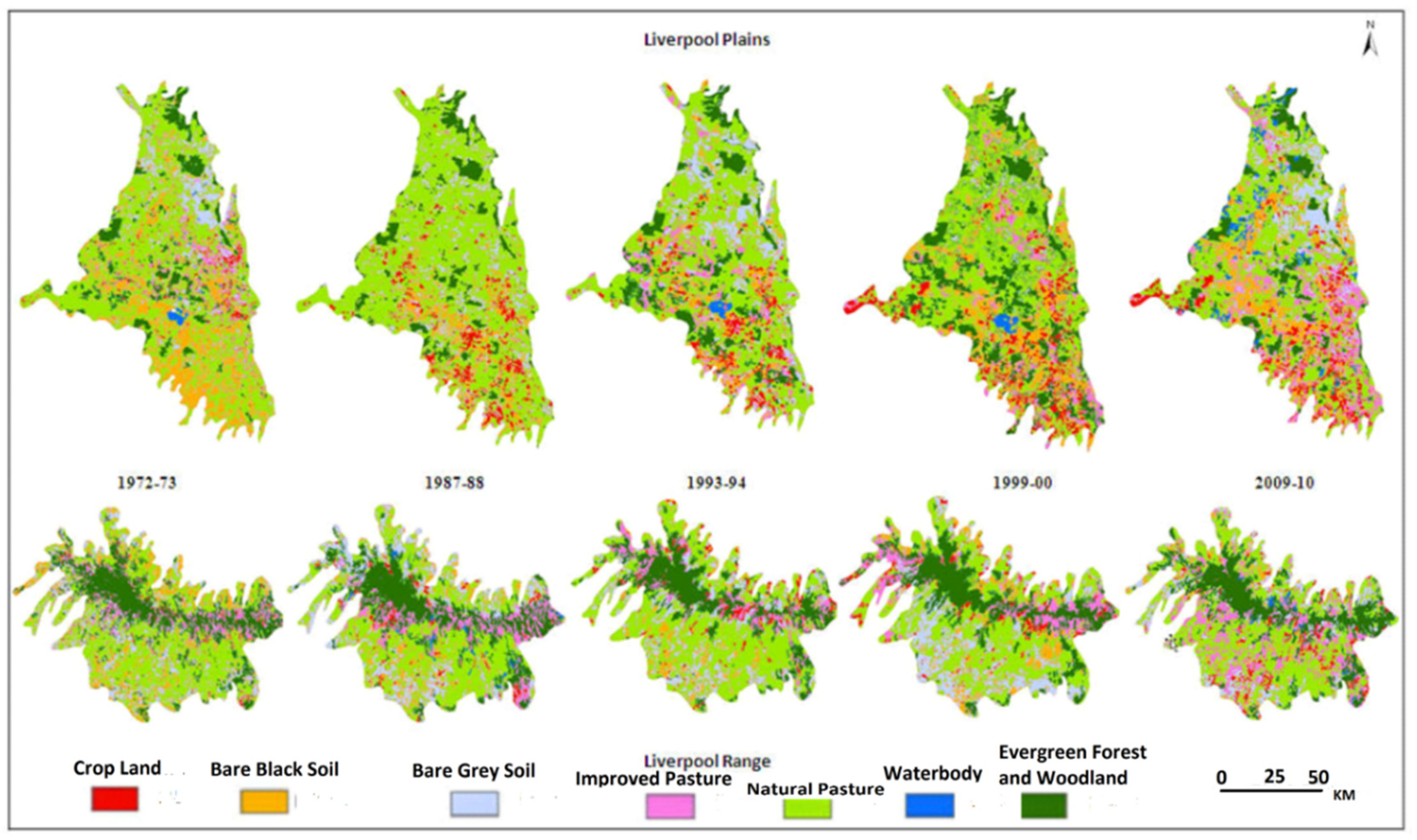
A Landsat Multi Spectral Scanner (MSS) scene of 1972–1973 and Thematic Mapper 5 (TM) scenes of 1987–1988, 1993–1994, 1999–2000 and 2009–2010 (mostly summer, December–February period) were selected. The images were referenced to Lambert’s Conformal Conic Projection. MSS 57-m pixels were resampled to 30-m pixel size in order to make them similar to TM pixels. TM bands 2, 3 and 4 were similar to corresponding MSS bands 4, 5 and 7 and hence the entire image processing was carried out on these selected bands. The images were segmented using eCognition software where pixels were merged into objects based on pixel spectral properties and defined scale parameters, set through a number of trials. Seven broad land cover classes, viz. Bare Black Soil (BBS), Bare Grey Soil (BGS), Cropland (CL), Native Pasture (NP), Improved Pasture (IP), Evergreen Forest and Woodland (EFWL) and Waterbody (WB), were identified. Fieldwork for training and validation sampling was conducted in November–December 2010 and in January 2011 using the Landsat image data, Google Earth high spatial resolution image prints and topographic maps as guides. Some 56–134 reference points were randomly selected for each class in the bioregion depending upon their extent and homogeneity. These points were confirmed during the GPS-based field survey conducted during the above-mentioned periods. Some 774 reference points were assessed and information regarding each point was noted throughout the study area in an effort to represent all identified land cover types and their variation across the region. Care was taken to note possible dynamic land cover types, such as agricultural classes that could have changed between image and field data acquisition dates. Sample point information collected in 2010–11 was used as the dependent sample for classification and accuracy evaluation for other change periods [40,41]. As no reference data were available for other change periods, the interpretation directly from the Landsat image was deemed to be too susceptible to error and user influence [40]. To use field reference data from 2010 to 2011 for accuracy evaluation in other change periods, additional processing was undertaken to include sites that had not changed during these periods. An image differencing technique was used to generate difference images for the above change periods with respect to the 2009 image using ±1 standard deviation (SD) as a threshold [42,43]. Unchanged pixels were usually clustered about the mean of the difference histogram distribution, while changed pixels were found in the tails. All 2010–2011 validation sites were assessed in comparison to the change images and sites that fell on areas greater than ±1 SD from the mean were discarded. The remaining sites were assumed to have not changed over time and were used as validation data for classifications.
After refinement, 707, 669, 596 and 530 sample points were left for the 1999, 1993, 1987 and 1972 images, respectively, for classification and accuracy evaluation. The nearest-neighbor method was applied with segmented object classification using refined sample sites randomly split into one third for training and two thirds for validation in each change period. Accuracy assessment, which is an integral part of any image classification process, was performed to estimate the accuracy of the land cover classifications using a method described by Congalton and co-authors [44,45,46]. Land cover classification accuracy from the 1972 MSS image was lower (overall accuracy, 76%; Kappa, 0.73) than that of the TM images in other years, for which a high overall accuracy (>86%) and Kappa (>0.85) were achieved. The classification outputs were used to generate land cover maps for both the LP and LR provinces. Figure 2 shows the LP and LR land cover maps in different years.
The landscape metrics were computed by means of a FRAGSTATS [13] (http://www.umass.edu/landeco/research/fragstats/documents/fragstats.help.4.2.pdf) interface with ARC/INFO (www.esri.com) software. Both landscape and class-level metrics were computed using land cover grids based on the eight-cell rule for patch neighbors, which takes into account both orthogonal and diagonal cells as neighbors [47] for the generation of patches. Thirty metrics were computed as discussed in Table 1.
Figure 2. Land cover classification in different years for the Liverpool Plains (LP) and Liverpool Range (LR) provinces (refer Section 3.1 for class descriptions).
Remotesensing 08 00107 g002
Table 1. List of landscape metrics used in this study [13]).
CodeNameTypeRank *CodeNameTypeRank *
NPNumber of patchesArea10NCANumber of core areasInterior25
CAClass area (ha)Area21TCATotal core area (ha)Interior19
LPILargest patch indexArea13CORE_MNMean core area per patch (ha)Interior1
AREA_MNMean patch size (ha)Area22CORE_SDPatch core area standard deviation (ha)Interior26
AREA_SDPatch size standard deviation (ha)Area15CORE_CVPatch core area coefficient of variation (%)Interior27
Area_CVPatch size coefficient of variation (%)Area23ENN_MNMean nearest neighbor distance (m)Isolation6
TETotal edge (m)Edge9PROX_MNMean proximity indexIsolation16
MPEMean patch edge (m)Edge24PRPatch richnessHeterogeneity5
PAR_AMMean perimeter/area ratioShape6SHDIShannon’s diversity indexHeterogeneity3
LSILandscape shape indexShape17SHEIShannon’s evenness indexHeterogeneity3
SHAPE_MNMean shape indexShape12MSIDIModified Simpson’s diversity indexHeterogeneity2
SHAPE_AWArea-weighted mean patch fractal dimensionShape8IJIInterspersion and juxtaposition index (%)Heterogeneity18
FRACFractal dimensionShape11AIAggregation index (%)Heterogeneity28
FRAC_MNMean patch fractal dimensionShape12CONTAGContagion indexDispersion7
FRAC_AWArea-weighted mean patch fractal dimensionShape8COHESIONPatch cohesion indexConnectivity14
* Described in Section 4.5.
The suitability of pattern metrics for land cover monitoring was evaluated by computing a score for each of the criteria in Section 1.1, based on a method called Max–Min/Max normalization. This provided a way to compare values that are measured using different scales for one or two landscapes. The methods for computing these scores are described in the following section.

3.2. Capability of Metrics to Capture Change in Landscape Pattern

For patch rich and poor landscapes, it has been hypothesized that effective metrics should distinguish between various land cover patterns by providing different values for the two landscapes. For example, the LP province is forest poor and the LR is forest rich, so the metrics should give different values for both landscapes. Similarly, different values can be expected from agriculture rich (LP) and poor (LR) areas. A β-score was calculated for each metric based on the formula given in Equation (1) [27,48].
β = M a x ( P R L P , P R L R ) M i n ( P R L P , P R L R ) M a x ( P R L P , P R L R )
where PRLP, PRLR are values of the pattern metrics in LP and LR, respectively, depending upon the class used. Similarly, it has also been assumed that, in case of land cover change over a given period, effective metrics should reflect change by returning a different value in different years. Based on this, a γ-score was computed for each metric for LP and LR to assess the ability of the metric to recognize temporal change, using Equation (2), related to the β-score [27,48].
γ = ( M a x ( T 1 , T 2 , T n ) M i n ( T 1 , T 2 , T n ) ) ( M a x ( T 1 , T 2 , T n ) )
where Max (T1, T2,…Tn) is the maximum value of a given metric for the n years. Metrics were computed in this study for the five change years (1972–1973, 1987–1988, 1993–1994, 1999–2000, and 2009–2010) for both LP and LR. Assuming that higher β and γ scores were more favorable in change identification, the metrics were ranked in descending order of both scores.

3.3. Sensitivity of Metrics to Spatial Resolution of Remote Sensing Data

Previous studies have shown that changing grain size has significant effects on the value of landscape metrics and that the magnitude and pattern of these responses varies among metrics and landscapes (e.g., [36,37,38]). In this study, the spatial resolution varied between 30 m and 60 m depending on whether images were TM or MSS. Resampling was carried out to make MSS pixels similar to TM pixels. In addition, raster data in GIS can be represented by an almost unlimited number of spatial resolutions. When using metrics that are sensitive to changes in measurement resolution, integrated investigations of landscape patterns that use multiple sensor data products may prove invalid [26]. The sensitivity of each metric to spatial resolution was assessed through the ξ-score, given in Equation (3) [48]. The original classification raster data were re-sampled to grids with 20, 30, 60 and 100-m pixel sizes.
ξ = ( M a x ( R 1 , R 2 , R n ) M i n ( R 1 , R 2 , R n ) ) M a x ( R 1 , R 2 , R n )
where R1, R2,…Rn are values of metrics with different pixel spatial resolutions (i.e., 20, 30, 60 and 100 m). The ξ-score was computed for each metric in each province and year.

3.4. Sensitivity of Metrics to Number of Classes

Several studies have indicated that the thematic resolution or the number of classes in a land cover map can affect different measures of landscape attribute and mapping accuracy (e.g., [49,50]). In the case of monitoring long-term land cover change in vegetated landscapes, the type and extent of different land cover types vary as classes change from one to another, mainly due to human-related activities. In such situations, it is necessary to assess the sensitivity of pattern metrics, used for change evaluation, to changing numbers of classes. The effect of these possible ontological changes was estimated by the θ-score [48]:
θ = ( M a x ( C L 1 , C L 2 , C L n ) M i n ( C L 1 , C L 2 , C L n ) ) M a x ( C L 1 , C L 2 , C L n )
where CL1, CL2,…CLn are the values of a given metric based on n land classes. In this study, metrics were computed for four different sets of land cover classes for both LP and LR in all years. The first set consisted of the original seven land cover classes (BBS, BGS, CL, IP, NP, EFWL and WB) as mentioned in Section 3.1. In the second set, land cover classes such as BBS, BGS, CL and IP were merged as agriculture land (AL) to make four land cover classes (AL, NP, EFWL and WB). The third set contained three land cover classes (AL, NV, WB) by merging NP and EFWL as natural vegetation (NV). The fourth and final set consisted of only two classes by merging all vegetation categories (CL, IP, NP, EFWL) into Vegetation (V) and BBS, BGS and WB into non-vegetation (NV) categories. Considering low ξ and θ-scores to be favorable for assessing change, the metrics were ranked in ascending order on these scores.

3.5. Statistical Analysis

A data matrix consisting of four scores, β and γ (ranked in descending order), and ξ and θ (ranked in ascending order) for each pattern metric and change period was analyzed using hierarchical cluster analysis (HCA) revealing natural groupings (or clusters) in the data. A correlation analysis was performed to exclude redundant metrics from further analysis as the number of available metrics was large (40) and many were presumed to be correlated [5,16]. Since the main issue here was not the redundancy of a metric itself but the duplication of change detected by these metrics, the absolute change in each metric value in different change periods (1972–1987, 1987–1993, 1993–1999 and 1999–2009) was analyzed using non-parametric Spearman correlations (ρ) at a 5% level of significance. In cases where two metrics were significantly correlated, one was discarded.
The selection of a subset of pattern metrics for change was undertaken based on criteria described in Section 1. Initially, each metric was ranked separately based on descending β and γ-scores and by ascending ξ and θ-scores, on the basis of their suitability for pattern change identification. In the next step, these ranks were summed for each metric and the sums were again ranked in ascending order. Metrics with a lower rank were assumed to be best in fulfilling the four criteria described in Section 1 and were kept for change analysis, while the metrics with a higher rank were discarded. Correlation analysis was carried out in the case of metrics with similar ranks and only one was retained for change analysis.

4. Results

In this section, results for landscape pattern metrics are presented for multiple time periods for the two distinct provinces, LR and LP, in the Brigalow Belt South Bioregion of NSW. Results for native vegetation are emphasized, as remnant vegetation plays an important role in defining landscape structure and fragmentation in the study region.

4.1. Cluster Analysis

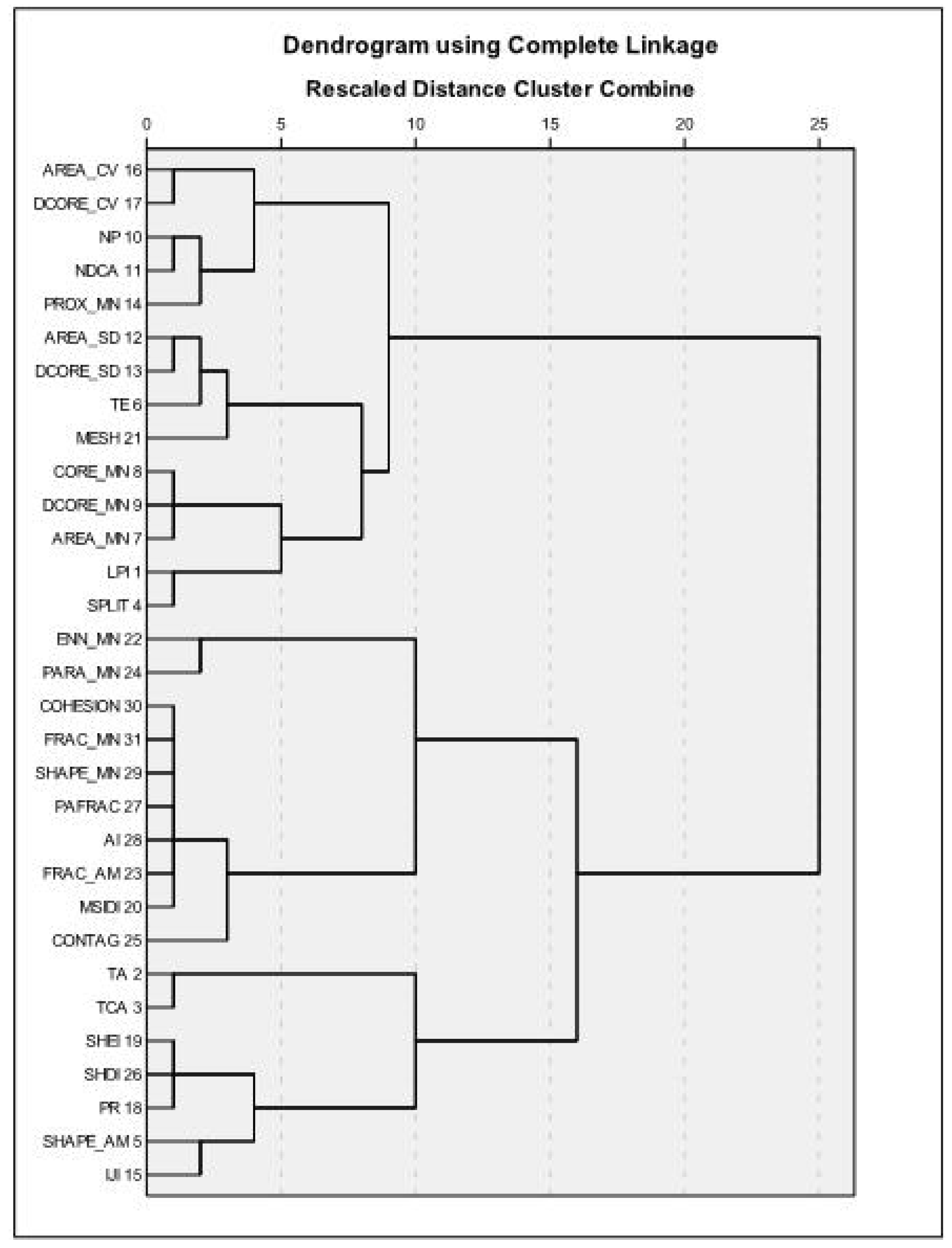
The result of the cluster analysis is shown in Figure 3. Five groups of metrics were resolved at a distance of five units between clusters. The first group contained mainly area, interior and isolation metrics while the second and third clusters consisted mainly of interior and edge metrics. The fourth cluster contained mainly shape metrics, while the fifth group consisted of spatial heterogeneity metrics.
Figure 3. Dendrogram of the hierarchal clustering of metrics.
Remotesensing 08 00107 g003

4.2. Analysis of β and γ-Scores of Metrics to Capture Landscape Pattern Change
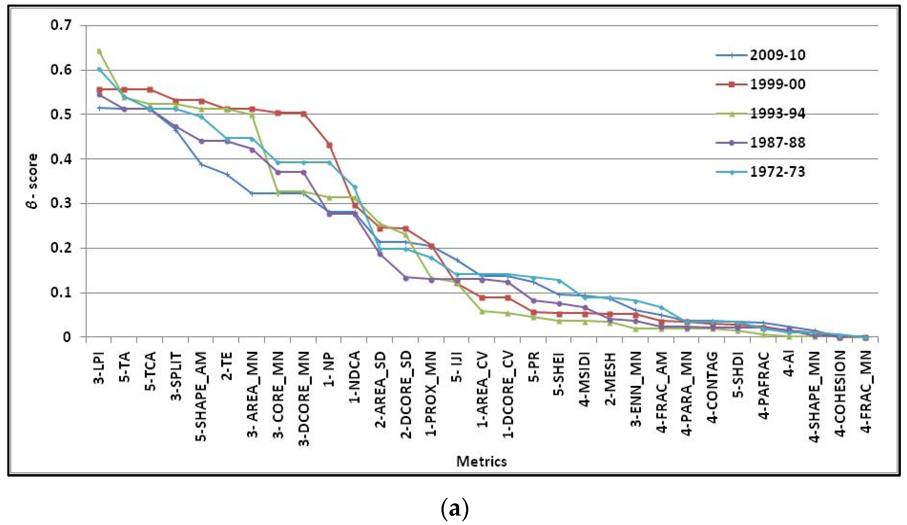
Figure 4a shows the ranked β-scores for each pattern metric based on comparison of values for the forest rich (LR) and poor (LP) provinces. A larger β-score implies greater capacity to identify a change in pattern. The rank order of β-scores was similar and the decrease in scores was more or less gradual for each year of imagery. Fourteen metrics (LPI, TA, SHAPE_AM, TE, AREA_MN, CORE_MN, DCORE_MN, NP, PROX_MN, AREA-CV, DCORE_CV, PR, SHEI, ENN_MN, MSIDI) showed consistently large differences between the two provinces in each change period. The remaining metrics had similarly low scores at each time, indicating a low capacity to discriminate different cover patterns.
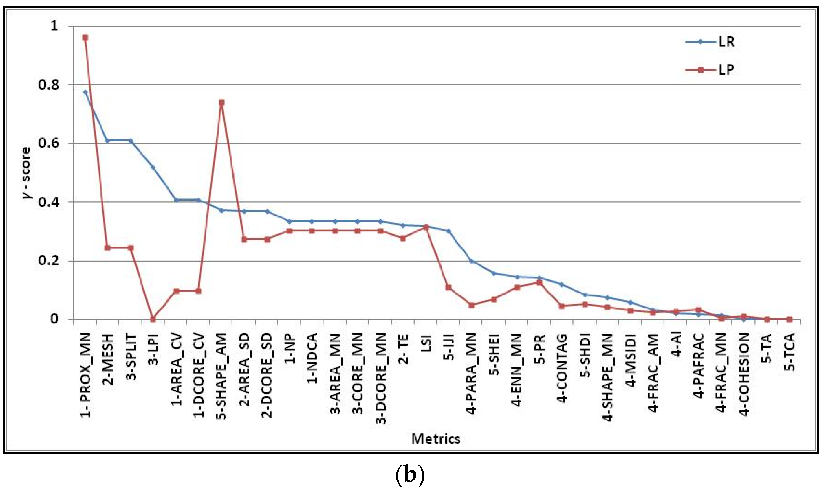
Figure 4. β-scores (a) and γ-scores (b), respectively, comparing the relative magnitude of each landscape metric in two contrasting provinces ranked in descending order for each of five change years (number before metric indicates cluster number, see Section 4.1). (See Table 1 for details of each metric).
Remotesensing 08 00107 g004aRemotesensing 08 00107 g004b
Most of the metrics that discriminated well between the two provinces belonged to clusters 2, 3 and 5, while the metrics in cluster 4 were characterized by low β-scores. However, the behavior of the metrics was not uniform in all change periods. That is, if a metric highlighted difference in values in the 1972–1987 period, the same metric did not necessarily highlight a difference in other change periods. A subset of selected metrics showed uniform differences in all change periods between the two landscapes (e.g., LPI, SHAPE_AM, AREA_MN, DCORE-SD, PR and SHEI) while the remaining metrics highlighted differences in only selected periods. For example, PROX-MIN showed a difference in 1972–1987 but not other periods. Similarly, TE did not highlight a difference in 1972–1987 and 1993–2000 but did so in other periods. The reason for such behavior can be attributed to the amount of change that occurred during different change periods, the amount of change being selectively captured by these metrics depending upon the quantity. A subset of selected metrics showing uniform differences in all change periods was selected based on β-scores.
Figure 4b shows the descending γ-scores computed for each pattern metric using values computed in each change year for both LP and LR. The γ-scores were ranked in descending order as larger values imply a higher capacity for change identification. Higher scores (γ ≥ 0.4) in LR were found for PROX_MN, MESH, SPLIT, LPI, AREA_CV, DCORE_CV and SHAPE_AM metrics. For LP, however, most of these metrics had lower scores, except for PROX_MN and SHAPE_AM, which were higher (γ ≥ 0.75) than their LR counterparts. For LP, these metrics were from all cluster groups except cluster 4, the metrics for which mostly fell in the right-hand part of the graph with much lower values. The remaining metrics showed a uniform decline in γ-value in the two landscapes. The metrics on the extreme right (mostly from cluster 4, except TA and TCA) showed no change in the two provinces over the entire change period (1972–2010).

4.3. Sensitivity of Metrics to Spatial Resolution of Remote Sensing Data
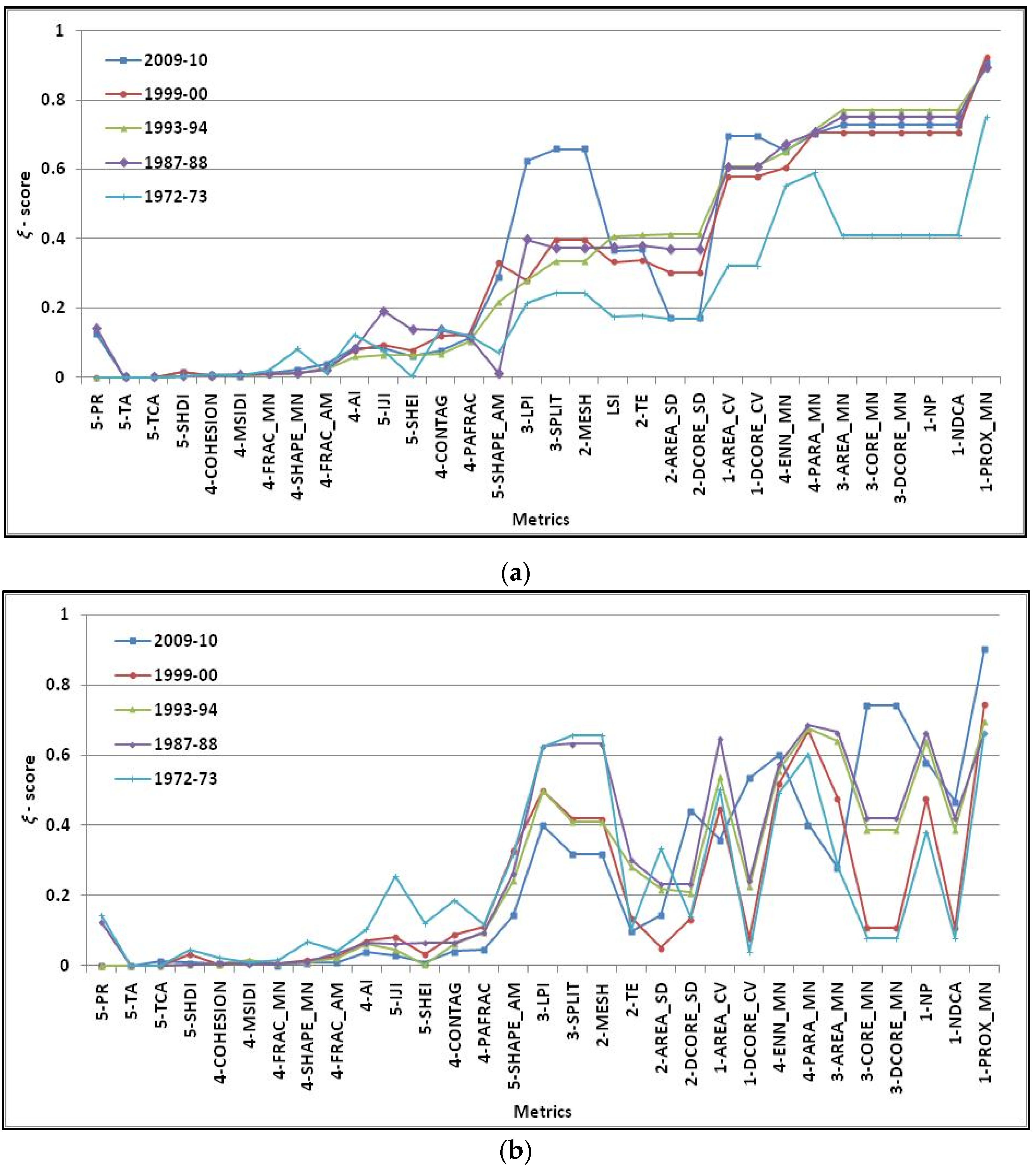
Pattern metric sensitivity towards change in spatial resolution varying from 20 to 100 m was assessed by ξ-scores for LR and LP provinces, respectively (Figure 5a,b). The values were ranked in ascending order and metrics with lower values were preferred considering their insensitivity to varying spatial resolution. In both cases, the metrics mostly from clusters 4 and 5, such as PR, TA, TCA, COHESION, SHDI, MSIDI, FRAC_MN, SHAPE_MN and FRAC_AM, were insensitive to pixel size. For metrics from clusters 2 and 3, intermediate values were found. Metrics such as AI, IJI, SHEI, CONTAG, PAFRAC, and SHAPE_AM varied by at least 20% in all years. Core area metrics, such as DCORE_SD, DCORE_CV, CORE_MN, and DCORE_MN were sensitive to spatial resolution, as were isolation measures, PROX_MN (cluster 1) and ENN_MN (cluster 4). The reasons for their sensitivity could be due to aggregation of smaller elongated patches lying between two or more larger patches as pixel size increases. In the case of LR, ξ-scores for metrics such as LPI, SPLIT, MESH, AREA_CV and DCORE_CV increased from 1972 to 2010, meaning that the sensitivity of these metrics to spatial resolution increased with time. Thus the low MSS spatial resolution data formed larger patch sizes by incorporating small size classes into one, compared to the TM data that formed a greater number of class patches. Thus as spatial resolution decreased from 20 to 100 m, class aggregation was more pronounced in the case of the TM data, leading to higher values. In other words, metrics from MSS classification were less spatially sensitive compared to those from TM data in the relatively homogeneous LR province. However, for the LP province (Figure 5b), these metrics showed the reverse trend, with sensitivities decreasing from 1972 to 2010. This was probably due to the heterogeneous nature of the LP province, where the MSS data formed smaller patch sizes (of fewer pixels) compared to TM images. Thus, with degrading pixel spatial resolution, the clumping of MSS pixels into neighboring classes became more pronounced (even with nearest neighborhood resampling techniques), making MSS data classifications spatially sensitive compared to those based on TM data.
Figure 5. (a,b) ξ-scores of landscape metrics ranked in ascending order for the Liverpool Range and Liverpool Plains, respectively. (number before metric indicates cluster number, see Section 4.1). (See Table 1 for details of each metric).
Remotesensing 08 00107 g005

4.4. Sensitivity of Metrics to Thematic Changes
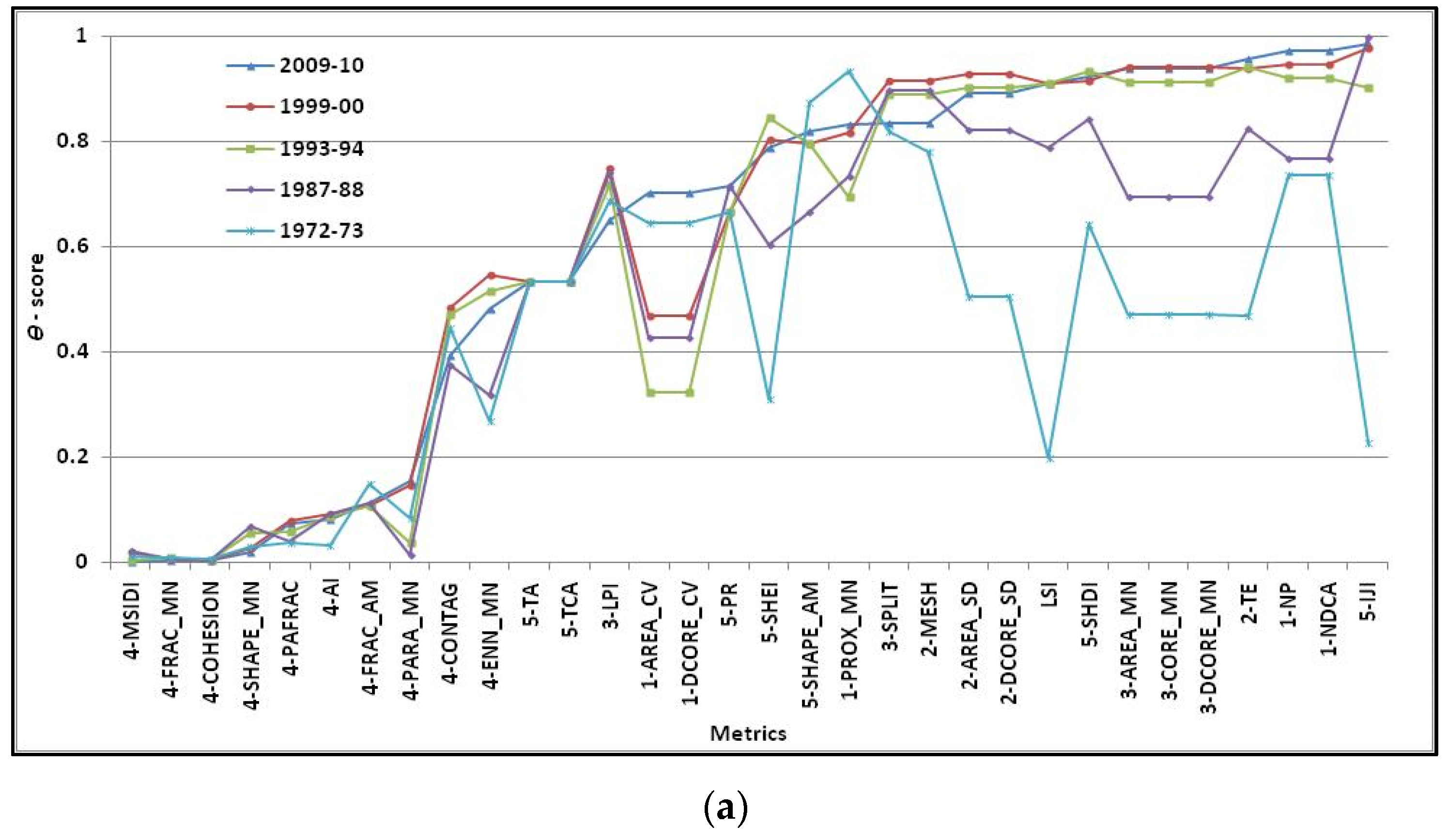
Thematic maps derived from remote sensing data have routinely been used to compute landscape metrics to quantify spatial pattern and temporal change in landscapes. It is imperative to understand what these metrics measure before appropriate interpretation of the results is possible. Although numerous studies in last two decades have reported the “behavior” of landscape metrics, very few studies have focused on the response of metrics to the changing thematic resolution of the mapped data (e.g., [10,51,52]). Changing the number of classes in categorical maps alters the spatial patterns, potentially resulting in different values for a given landscape metric. Li and Wu [10] illustrated how the level of classification detail could affect several landscape indices. Wu et al. [36], Wu [37] and Shen et al. [38] showed that the number of classes influenced scaling relations in landscape metrics. Li and Reynolds [51] found a relationship between number of patch types and contagion. Buyantuyev and Wu [50] showed that varying thematic resolution significantly affected landscape metric values and, in turn, the ability of these metrics to detect landscape change. The present study assumes that the sensitivity of a landscape metric to thematic resolution is proportional to the θ-score, computed as the difference between the maximum and minimum values generated with differing numbers of cover classes, relative to the maximum value (Equation (4)).
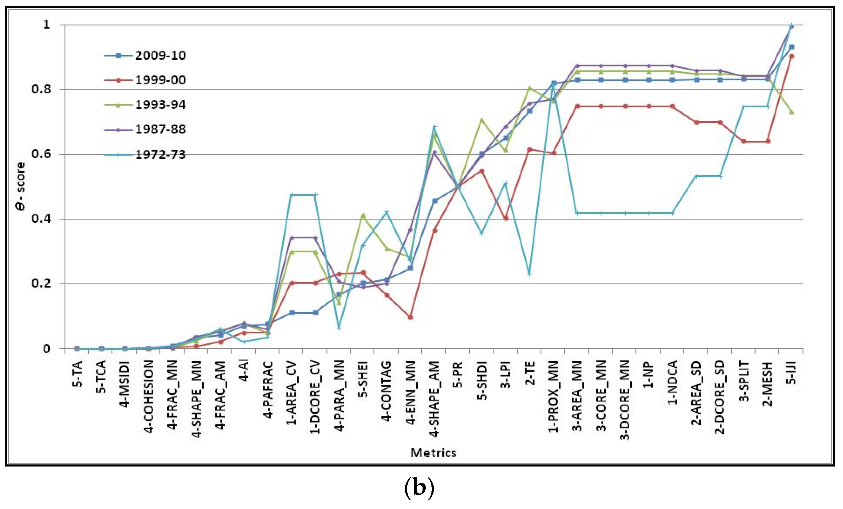
The sensitivity of pattern metrics to thematic resolution, computed as θ-scores in different years for LR and LP, are shown in Figure 6a,b, respectively. The values were ranked in ascending order and the lower values were considered insensitive to the number of classes. The hypothesis was based on the observations that decreasing the thematic resolution leads to a consistent decrease in the number of classes. For both LR and LP, metrics with lower θ-scores (<0.5) were in clusters 4 and 5, mainly consisted of shape (FRACT_MN, SHAPE_MN, PAFRAC, FRAC_AM, and PARA_MN) and heterogeneity metrics, such as AI and MSIDI, and registered least impact of thematic resolution. Buyantuyev and Wu [50] also found PAFD, MPSI, and MPFD to be insensitive towards thematic resolution. In general, the response patterns of most landscape metrics to changing thematic resolution seemed similar among different years.
Figure 6. (a,b) θ-score of landscape metrics for the Liverpool Range and Liverpool Plains, respectively, in different years (number before metric indicates cluster number, see Section 4.1). (See Table 1 for details of each metric).
Remotesensing 08 00107 g006aRemotesensing 08 00107 g006b
Higher values (i.e., higher sensitivity) observed in cluster 2 and 3 metrics, mostly related to area and interior categories, except for TA and TCA. Higher θ-scores were also found for ENN_MN, PROX_MN and IJI, indices describing the degree of isolation and interspersion of class patches. This can be explained by the fact that, when a larger number of patch types is chosen, the probability that two neighboring patches are of the same type decreases [27]. Patches of the same type are thus further apart, causing higher isolation. The sensitivity of metrics to thematic resolution increased from 1972 to 2010 in both LR and LP provinces in most cases.

4.5. Selection of Landscape Metrics

Table 1 shows the ranks for the different metrics. The low-ranked metrics were best in fulfilling the four criteria described in Section 1 and were kept for change analysis, while the metrics with higher ranks were discarded. Some 15 metrics were selected from different groups after this process, including the area distribution metrics, NP and AREA_MN, and the edge group metrics, TE and PAR_MN. In the group of shape indices, several metrics were acceptable, such as SHAPE_AW, FRACT_AW, FRACT_AW and LSI, while from the interior-edge metric group, CORE_MN and CORE_CV were suitable. Isolation was best expressed by ENN_MN. Finally, for studying heterogeneity, PR, SHDI, SHEI and MSIDI were selected. Since NP and MPS were correlated with each other, they contained redundant information. NP was preferred since this metric was only correlated with four other metrics, while AREA_MN was correlated with five. The shape indices were mutually correlated, as well. LSI was correlated with seven other metrics, PAR_MN with five and both SHAPE_MN and FRACT_AW with three. Since SHAPE_MN had the highest ranking, this was considered the best choice to describe shape complexity. Similarly among the heterogeneity measures, PR was correlated with six other metrics, SHEI with five and both SHDI and MSIDI with four. MSIDI, being the least correlated with others, was preferred to characterize landscape heterogeneity. The final group of eight metrics with least redundancy consisted of MSIDI, SHAPE_AM, CORE_MN, TE, NP, CONTAG, ENN_MN and FRAC_MN.

4.6. Change Analysis Using the Two Study Sites
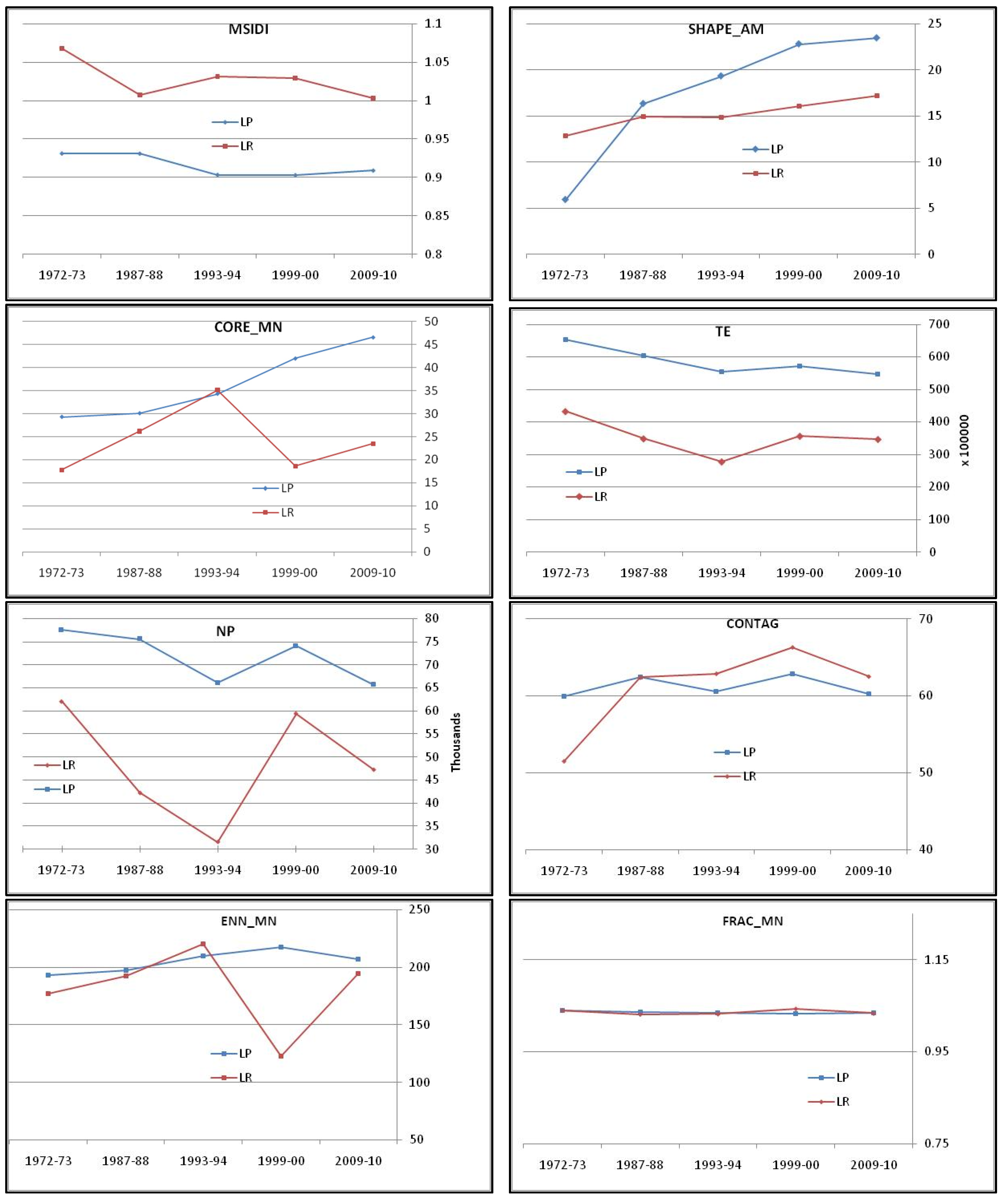
To compare change over time in each province, eight metrics were calculated for each change period, from 1972 to 2009 (Figure 7). In both provinces, NP decreased from 1972 to 1993, then increased between 1993 and 1999 and again decreased between 1999 and 2009. The increase in NP was more pronounced in LP. A similar pattern of change in TE was observed in the two landscapes. Landscape patches became more intact with less patch edge due to thickening of woodlands and maturation of planted trees over time. However, a rapid increase in NP and TE indicated greater fragmentation in both LP and LR during 1993–1999. The reasons for these increases were mostly due to clearing of native vegetation (woodlands and native pasture) in the two provinces. This fact is supported by Pressey et al. [53] and the 2000 New South Wales State of the Environment Report [54]: although much of the native vegetation in the bioregion had been cleared earlier in European settlement, 2.2% of the bioregion was cleared between 1997 and 2000 after the introduction of the Native Vegetation Conservation (NVC) Act 1997 (NSW), which provided an assessment and development consent process in relation to the clearing of native vegetation.
Figure 7. Changes in pattern metrics through time for the Liverpool Plains and the Liverpool Range. (See Table 1 for details of each metric).
Remotesensing 08 00107 g007
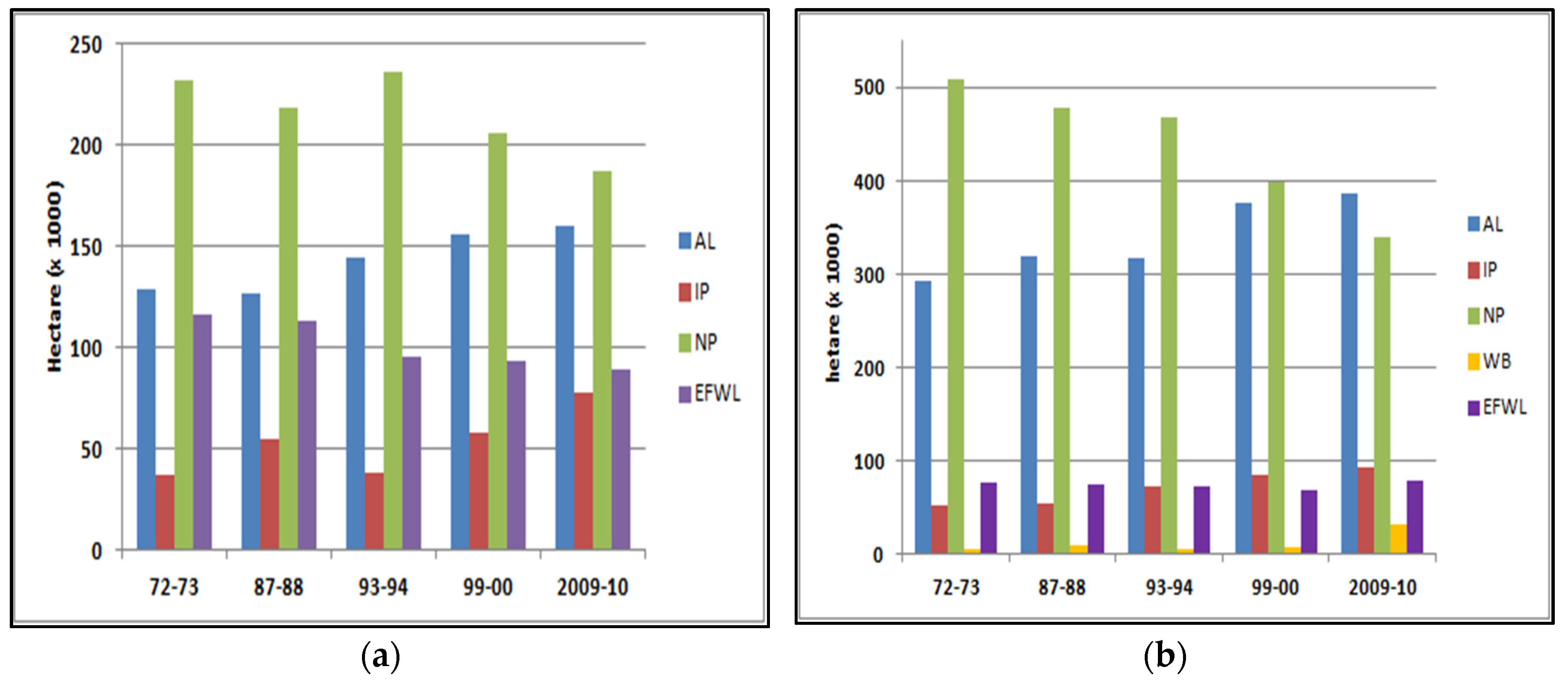
The largest amount of change was clearing (with retention of individual trees or clumps of trees), for the purposes of cropping and grazing in the period 1995–2000 [39]. Some 8.7% and 15.6% of the area of native vegetation was cleared in LP and LR, respectively, during this period. The land cover area statistics generated for the two provinces in different years are shown in Figure 8. Natural vegetation (NP and EFWL) cover declined in the two provinces over the study period, with the most marked decline after 1993. At the same time the area of agriculture-related activities increased. Although the number of patches and edges decreased between 1999 and 2009 (decreasing NP and TE values), the two landscapes appeared to be irregularly shaped as indicated by increasing SHAPE_AW values during this period. Increasing mean patch core area from 1973 to 1993 indicated only smaller patches were subject to fragmentation, but, after 1993, larger patches were also fragmented as shown by decreasing core area values. The CONTAG values showed a zig-zig increasing and decreasing trend from 1972 to 2010 and provided an effective summary of overall aggregation of the different land cover categories. Again, the highest values for the two landscapes were observed between 1993 and 1999 showing fragmentation of larger patches into smaller patches due to clearing of native vegetation as explained above. Between 1972 and 1993, a gradual increase in ENN_MN indicated that smaller patches were continuously cleared and became isolated in the two landscapes. The decline in ENN_MN in LR after 1993 indicated that smaller patches remained intact but were cleared after 1999, as the metric increased. However, in LP, the values increased after 1993, with a slight improvement only after 1999. Different class types did not intermix much over the entire period in either province as MSIDI was almost invariant. Overall, the comparison of metrics in the two provinces indicated major changes in land cover pattern after 1993, and though the trends were similar in both cases, remnant native vegetation in the LP province was more fragmented than in the LR province.
Figure 8. Land cover from 1972–1973 to 2009–2010 in the (a) Liverpool Range; and (b) Liverpool Plains provinces.
Remotesensing 08 00107 g008

5. Discussion

Understanding and evaluation of trends in land cover change, such as landscape fragmentation, can be best represented by spatial pattern metrics. However, the choice and interpretation of the most appropriate metrics to effectively represent landscape change is often challenging as all landscape metrics suffer from limitations that restrict their use and interpretation in different contexts [13]. Metrics can be selected based on multivariate data analysis techniques, but they are not useful in practical applications. There is a need for a simple straightforward approach to evaluate landscape metrics with respect to spatial data characteristics, such as metric behavior in relation to variation in spatial and temporal resolution, number of land cover classes or dominant land cover categories, measurement techniques and their inter-correlations, spatial scale, and so on, and for effective metric selection without needing to consider theoretical or advanced modeling issues. . Previous studies have considered some of these issues (e.g., [26,27,28]), but detailed analyses are required to fully explain the strengths and weaknesses of the multitude of different metrics in relation to data characteristics. Effective pattern metrics should only be sensitive to real spatial patterns and insensitive to random sampling variation [27].
Keeping the above facts in mind, this study applied a relatively simple and effective approach to select pattern metrics for land cover change detection. The selection process was carried out according to four criteria—each metric should be: (a) capable of capturing changes in landscape pattern in space and time; (b) insensitive to the spatial resolution of the remote sensing data; (c) insensitive to the number of land cover classes; and (d) minimally correlated with other metrics. This study hypothesized that an effective metric selection process based on the above criteria should distinguish between land cover patterns by providing different values for divergent spatial characteristics (e.g., differing spatial and temporal patterns, thematic resolutions, dominant land cover categories and extent) in two distinct landscapes. The hypothesis was tested through computation of four (β, γ, ξ and θ) relative difference-based indices using a Max–Min/Max normalization approach. This facilitated comparison of metrics measured on different scales in relation to one or two landscapes. Additionally, we wanted to know which metrics best answer the demands of spatial pattern monitoring. The choice of metric should be based on the particular questions being asked as a metric cannot satisfy all conditions simultaneously. The selected metrics fulfilled the criteria described in Section 3.1, particularly the capability of capturing changes in landscape pattern over space and time. For example, number of patches (NP) and Total Edge (TE) decreased over the change periods (except between 1993 and 1999), indicating a general trend towards consolidation of patches in the landscape due to thickening of woodlands and maturation of planted trees over time. However, a rapid increase in NP and TE values between 1993 and 1999 indicated greater loss of native vegetation or more fragmentation in both the LP and LR provinces. Even though NP and TE values decreased over 1999–2009 period, increasing SHAPE_AW values indicated the two landscapes became more irregularly shaped. Similarly, increasing mean patch core area from 1973 to 1993 indicated fragmentation of smaller patches, but after 1993, larger patches were also fragmented as shown by decreasing core area values. The CONTAG values showed a zig-zig increasing and decreasing trend describing overall aggregation of the different land cover categories. Increase in ENN_MN between 1972 and 1993 indicated continuous clearing of smaller patches, while decline in ENN_MN in LR after 1993 indicated that smaller patches remained intact but were cleared after 1999, as the metric increased. However, in LP, the values increased after 1993, with a slight improvement only after 1999. Intermixing between different class types did not occur much over the entire period in either province as MSIDI was almost invariant. Comparison of the metrics in the two provinces in the NSW case study indicated major changes in land cover pattern after 1993 in relation to clearance of remnant native vegetation and transformation for agriculture. Although the trend was similar in both cases, the Liverpool Plains province was more fragmented than the Liverpool Ranges.
The accuracy of the land cover data used in change detection analysis can have a large impact on the change outcome. Estimates of future land cover change may be biased and inaccurate if ether are errors in land cover classification. Therefore, understanding and quantifying uncertainties in observed land cover change and the possible impact of such errors over time are important in land cover change studies. Fang et al. [55] found that classification errors were a major source of uncertainty in model predictions. Assuming the errors in “before” and “after” maps are independent, the overall accuracy of a change map can be approximated by multiplying the individual overall accuracy of each map [46]. Thus, in the present case study, if the overall accuracy of the 1972 and 1987 map was 76% and 86%, respectively, the 1972–1987 change map is 62% accurate and the change maps for other periods are 74% accurate. It can therefore be assumed that misclassification errors in the resulting land cover change maps based on MSS (76%) and TM (86%) imagery and from the other TM images (with an overall accuracy >86%) would affect the change results. Therefore, to increase the reliability of change maps, misclassification errors in land use maps should be minimized. Carmel and Dean [56] developed an error model to calculate uncertainly propagation within classified spatio-temporal datasets. Congalton and Green [46] proposed a two-step change detection accuracy assessment process to assess the accuracy with which the change area between two time periods is mapped and the change captured. The task of quantifying these errors and developing an understanding of how they propagate over time is challenging; however, this information is important for change prediction modeling and merits further study. The change results here can be interpreted based on the respective accuracies of each change period, and the results improved with more accurate maps following the method suggested by Congalton and Green [46] in future studies.

6. Conclusions

The study evaluated landscape metrics with respect to remote sensing data characteristics, such as their behavior in relation to variation in spatial and temporal resolution, number of land cover classes or dominant land cover categories. The proposed rank-based metric selection process through computation of four difference-based indices (β, γ, ξ and θ) using a Max–Min/Max normalization ascertained that change in a metric was due to real landscape pattern change. The selected landscape metrics were successful and effective in detecting land cover pattern change in two contrasting landscapes.
The pattern of change agreed with results reported previously in the region based on other methods [39]. The metrics identified were capable of identifying changes over five different change periods in provinces with contrasting topography, woodland and forests, and agricultural land uses. The approach is straightforward, simple and effective for identifying the most suitable landscape metrics for pattern change analysis in landscape ecology. The methods can be used in any landscape under any conditions, and can potentially deal with hundreds of metrics when selection of an appropriate set of metrics by other means would be logistically difficult.

Author Contributions

Conceived and designed the experiments: Priyakant Sinha, Lalit Kumar. Performed the experiments: Priyakant Sinha. Analysed the data: Priyakant Sinha, Lalit Kumar, Nick Reid. Wrote the paper: Priyakant Sinha, Lalit Kumar, Nick Reid.

Conflicts of Interest

The authors declare no conflict of interest.

References

  1. Read, J.; Lam, N.S. Spatial methods for characterising land cover and detecting land-cover changes for the tropics. Int. J. Remote Sens. 2002, 23, 2457–2474. [Google Scholar] [CrossRef]
  2. McGarigal, K.; Romme, W.H.; Crist, M.; Roworth, E. Cumulative effects of roads and logging on landscape structure in the San Juan Mountains, Colorado (USA). Landsc. Ecol. 2001, 16, 327–349. [Google Scholar] [CrossRef]
  3. Leimgruber, P.; Mcshea, W.J.; Schnell, G.D. Effects of scale and logging on landscape structure in a forest mosaic. Environ. Monit. Assess. 2002, 74, 141–166. [Google Scholar] [CrossRef] [PubMed]
  4. Arnot, C.; Fisher, P.F.; Wadsworth, R.; Wellens, J. Landscape metrics with ecotones: Pattern under uncertainty. Landsc. Ecol. 2004, 19, 181–195. [Google Scholar] [CrossRef]
  5. Griffith, J.A.; Martinko, E.A.; Price, K.P. Landscape structure analysis of Kansas at three scales. Landsc. Urban Plan. 2000, 52, 45–61. [Google Scholar] [CrossRef]
  6. Fuller, D.O. Forest fragmentation in Loudoun County, Virginia, USA evaluated with multitemporal Landsat imagery. Landsc. Ecol. 2001, 16, 627–642. [Google Scholar] [CrossRef]
  7. Liu, A.J.; Cameron, G.N. Analysis of landscape patterns in coastal wetlands of Galveston Bay, Texas (USA). Landsc. Ecol. 2001, 16, 581–595. [Google Scholar] [CrossRef]
  8. Botequilha Leitão, A.; Ahern, J. Applying landscape ecological concepts and metrics in sustainable landscape planning. Landsc. Urban Plan. 2002, 59, 65–93. [Google Scholar] [CrossRef]
  9. Gergel, S.E. Spatial and non-spatial factors: When do they affect landscape indicators of watershed loading? Landsc. Ecol. 2005, 20, 177–189. [Google Scholar] [CrossRef]
  10. Li, H.; Wu, J. Use and misuse of landscape indices. Landsc. Ecol. 2004, 19, 389–399. [Google Scholar] [CrossRef]
  11. Turner, M.G.; Gardner, R.H.; O’Neill, R.V. Landscape Ecology in Theory and Practice; Springer-Verlag: New York, NY, USA, 2001. [Google Scholar]
  12. Lindenmayer, D.B.; Cunningham, R.B.; Donnelly, C.F.; Lesslie, R. On the use of landscape surrogates as ecological indicators in fragmented forests. For. Ecol. Manag. 2002, 159, 203–216. [Google Scholar] [CrossRef]
  13. McGarigal, K.; Marks, B.J. Spatial Pattern Analysis Program for Quantifying Landscape Structure; Gen. Tech. Rep. PNW-GTR-351; US Department of Agriculture, Forest Service, Pacific Northwest Research Station: Portland, OR, USA, 1995. [Google Scholar]
  14. Rempel, R.S.; Carr, A.; Elkie, P.C. Patch Analyst User’s Manual: A Tool for Quantifying Landscape Structure; Ontario Ministry of Natural Resources, Boreal Science, Northwest Science & Technology: Thunder Bay, ON, Canada, 1999.
  15. Crews-Meyer, K.A. Characterizing landscape dynamism using pane-pattern metrics. Photogramm. Eng. Remote Sens. 2002, 68, 1031–1040. [Google Scholar]
  16. Cumming, S.; Vervier, P. Statistical models of landscape pattern metrics, with applications to regional scale dynamic forest simulations. Landsc. Ecol. 2002, 17, 433–444. [Google Scholar] [CrossRef]
  17. Stanfield, B.J.; Bliss, J.C.; Spies, T.A. Land ownership and landscape structure: A spatial analysis of sixty-six Oregon (USA) Coast Range watersheds. Landsc. Ecol. 2002, 17, 685–697. [Google Scholar] [CrossRef]
  18. Riitters, K.H.; O’neill, R.; Hunsaker, C.; Wickham, J.D.; Yankee, D.; Timmins, S.; Jones, K.; Jackson, B. A factor analysis of landscape pattern and structure metrics. Landsc. Ecol. 1995, 10, 23–39. [Google Scholar] [CrossRef]
  19. Cain, D.H.; Riitters, K.; Orvis, K. A multi-scale analysis of landscape statistics. Landsc. Ecol. 1997, 12, 199–212. [Google Scholar] [CrossRef]
  20. McAlpine, C.A.; Eyre, T.J. Testing landscape metrics as indicators of habitat loss and fragmentation in continuous eucalypt forests (Queensland, Australia). Landsc. Ecol. 2002, 17, 711–728. [Google Scholar] [CrossRef]
  21. Honnay, O.; Piessens, K.; van Landuyt, W.; Hermy, M.; Gulinck, H. Satellite based land use and landscape complexity indices as predictors for regional plant species diversity. Landsc. Urban Plan. 2003, 63, 241–250. [Google Scholar] [CrossRef]
  22. Schmitz, M.; de Aranzabal, I.; Aguilera, P.; Rescia, A.; Pineda, F. Relationship between landscape typology and socioeconomic structure: Scenarios of change in Spanish cultural landscapes. Ecol. Model. 2003, 168, 343–356. [Google Scholar] [CrossRef]
  23. Gustafson, E.J. Quantifying landscape spatial pattern: What is the state of the art? Ecosystems 1998, 1, 143–156. [Google Scholar] [CrossRef]
  24. Griffith, J.; Stehman, S.; Sohl, T.; Loveland, T. Detecting trends in landscape pattern metrics over a 20-year period using a sampling-based monitoring programme. Int. J. Remote Sens. 2003, 24, 175–181. [Google Scholar] [CrossRef]
  25. Civco, D.L.; Hurd, J.D.; Wilson, E.H.; Arnold, C.L.; Prisloe, M.P. Quantifying and describing urbanizing landscapes in the Northeast United States. Photogramm. Eng. Remote Sens. 2002, 68, 1083–1090. [Google Scholar]
  26. Frohn, R.C. Remote Sensing for Landscape Ecology: New Metric Indicators for Monitoring, Modeling, and Assessment of Ecosystems; CRC Press: Boca Raton, FL, USA, 1997. [Google Scholar]
  27. DeClercq, E.M.; Vandemoortele, F.; DeWulf, R.R. A method for the selection of relevant pattern indices for monitoring of spatial forest cover pattern at a regional scale. Int. J. Appl. Earth Obs. Geoinf. 2006, 8, 113–125. [Google Scholar] [CrossRef]
  28. Lechner, A.M.; Langford, W.T.; Jones, S.D.; Bekessy, S.A. Are landscape ecologists addressing uncertainty in their remote sensing data? Landsc. Ecol. 2012, 27, 1249–1261. [Google Scholar] [CrossRef]
  29. O’Neill, R.; Krummel, J.; Gardner, R.; Sugihara, G.; Jackson, B.; DeAngelis, D.; Milne, B.; Turner, M.; Zygmunt, B.; Christensen, S.; et al. Indices of landscape pattern. Landsc. Ecol. 1988, 1, 153–162. [Google Scholar] [CrossRef]
  30. Bogaert, J. Response to Bissonette JA and Storch I. 2002: “Fragmentation: Is the message clear?”—Lack of agreement on fragmentation metrics blurs correspondence between fragmentation experiments and predicted effects. Conserv. Ecol. 2003, 7, r6. [Google Scholar]
  31. Wickham, J.D.; O’Neill, R.V.; Ritters, K.H.; Wade, T.G.; Jones, K.B. Sensitivity of selected landscape pattern metrics to land-cover misclassification and differences in land-cover composition. Photogramm. Eng. Remote Sens. 1997, 63, 397–402. [Google Scholar]
  32. Saura, S. Effects of minimum mapping unit on land cover data spatial configuration and composition. Int. J. Remote Sens. 2002, 23, 4853–4880. [Google Scholar] [CrossRef]
  33. Saura, S. Effects of remote sensor spatial resolution and data aggregation on selected fragmentation indices. Landsc. Ecol. 2004, 19, 197–209. [Google Scholar] [CrossRef]
  34. Turner, M.G.; O’Neill, R.V.; Gardner, R.H.; Milne, B.T. Effects of changing spatial scale on the analysis of landscape pattern. Landsc. Ecol. 1989, 3, 153–162. [Google Scholar] [CrossRef]
  35. Saura, S.; Martinez-Millan, J. Sensitivity of landscape pattern metrics to map spatial extent. Photogramm. Eng. Remote Sens. 2001, 67, 1027–1036. [Google Scholar]
  36. Wu, J.; Shen, W.; Sun, W.; Tueller, P.T. Empirical patterns of the effects of changing scale on landscape metrics. Landsc. Ecol. 2002, 17, 761–782. [Google Scholar] [CrossRef]
  37. Wu, J. Effects of changing scale on landscape pattern analysis: Scaling relations. Landsc. Ecol. 2004, 19, 125–138. [Google Scholar] [CrossRef]
  38. Shen, W.; Jenerette, G.D.; Wu, J.; Gardner, R.H. Evaluating empirical scaling relations of pattern metrics with simulated landscapes. Ecography 2004, 27, 459–469. [Google Scholar] [CrossRef]
  39. Bioregional Conservation Assessment Scoping Report (BCASR). Brigalow Belt South, NSW, Bioregional Conservation Assessment Scope Report, Western Regional Assessments Unit, NSW National Parks and Wildlife Service, Dabbo, NSW 2830, 2002. Available online: http//www.nsw.gov.au (accessed on 15 October 2014).
  40. Foody, G.M. Thematic map comparison: Evaluating the statistical significance of differences in classification accuracy. Photogramm. Eng. Remote Sens. 2004, 70, 627–634. [Google Scholar] [CrossRef]
  41. Foody, G.M. Harshness in image classification accuracy assessment. Int. J. Remote Sens. 2008, 29, 3137–3158. [Google Scholar] [CrossRef]
  42. Sinha, P.; Kumar, L. Independent two step thresholding of binary images in inter-annual land cover change/no-change identification. ISPRS J. Photogramm. Eng. Remote Sens. 2013, 81, 31–43. [Google Scholar] [CrossRef]
  43. Sinha, P.; Kumar, L. Binary images in seasonal land-cover change identification: A comparative study in parts of NSW, Australia. Int. J. Remote Sens. 2013, 34, 2162–2182. [Google Scholar] [CrossRef]
  44. Congalton, R.G.; Oderwald, R.G.; Mead, R.A. Assessing Landsat classification accuracy using discrete multivariate analysis statistical techniques. Photogramm. Eng. Remote Sens. 1983, 49, 1671–1678. [Google Scholar]
  45. Congalton, R.G. A review of assessing the accuracy of classifications of remotely sensed data. Remote Sens. Environ. 1991, 37, 35–46. [Google Scholar] [CrossRef]
  46. Congalton, R.G.; Green, K. Assessing the Accuracy of Remotely Sensed Data: Principle and Practices, Mapping Science Series; Lewis Publications; CRC Press: Boca Raton, FL, USA, 2009. [Google Scholar]
  47. Rocchini, D.; Perry, G.L.W.; Salerno, M.; Maccherini, S.; Chiarucci, A. Landscape change and the dynamics of open formations in a natural reserve. Landsc. Urban Plan. 2006, 77, 167–177. [Google Scholar] [CrossRef]
  48. Vanddemoortele, F. Analyse Van Bosversnippering in Vlaanderen: Evaluatie Van Landschapsindices. Master’s Thesis, Ghent University, Gent, Belgium, 2004. [Google Scholar]
  49. Neel, M.C.; McGarigal, K.; Cushman, S.A. Behavior of class-level landscape metrics across gradients of class aggregation and area. Landsc. Ecol. 2004, 19, 435–455. [Google Scholar] [CrossRef]
  50. Buyantuyev, A.; Wu, J. Effects of thematic resolution on landscape pattern analysis. Landsc. Ecol. 2007, 22, 7–13. [Google Scholar] [CrossRef]
  51. Li, H.; Reynolds, J.F. A new contagion index to quantify spatial patterns of landscapes. Landsc. Ecol. 1993, 8, 155–162. [Google Scholar] [CrossRef]
  52. Baldwin, D.J.B.; Weaver, K.; Schnekenburger, F.; Perera, A.H. Sensitivity of landscape pattern indices to input data characteristics on real landscapes: Implications for their use in natural disturbance emulation. Landsc. Ecol. 2004, 19, 255–271. [Google Scholar] [CrossRef]
  53. Pressey, R.; Hager, T.; Ryan, K.; Schwarz, J.; Wall, S.; Ferrier, S.; Creaser, P. Using abiotic data for conservation assessments over extensive regions: Quantitative methods applied across New South Wales, Australia. Biol. Conserv. 2000, 96, 55–82. [Google Scholar] [CrossRef]
  54. Environmental Protection Authority. NSW Environmental Protection Authority 2000, NSW State of the Environment Report 2000. Environmental Protection Authority, Sydney. Available online: http://www.epa.nsw.gov.au (accessed on 23 August 2014).
  55. Fang, S.; Wente, S.; Gertner, G.Z.; Wang, G.; Anderson, A. Uncertainty analysis of predicted disturbance from offroad vehicular traffic in complex landscapes at Fort Hood. Environ. Manag. 2002, 30, 199–208. [Google Scholar] [CrossRef] [PubMed]
  56. Carmel, Y.; Dean, D.J. Performance of a spatio-temporal error model for raster datasets under complex error patterns. Int. J. Remote Sens. 2004, 25, 5283–5296. [Google Scholar] [CrossRef]