Simple Summary
- -
- A novel algorithm delivering high resolution soil moisture maps is developed by merging active (SAR) and passive microwave.
- -
- MAPSM is based on the concept ofWater Change Capacity.
- -
- A case study using MAPSM is presented by using the RADARSAT-2 and SMOS retrieved soil moisture data products over Berambadi watershed, Karnataka, India.
- -
- The algorithm parameters show scalability from the spatial resolution of 20 m to 2000 m.
Abstract
Availability of soil moisture observations at a high spatial and temporal resolution is a prerequisite for various hydrological, agricultural and meteorological applications. In the current study, a novel algorithm for merging soil moisture from active microwave (SAR) and passive microwave is presented. The MAPSM algorithm—Merge Active and Passive microwave Soil Moisture—uses a spatio-temporal approach based on the concept of the Water Change Capacity (WCC) which represents the amplitude and direction of change in the soil moisture at the fine spatial resolution. The algorithm is applied and validated during a period of 3 years spanning from 2010 to 2013 over the Berambadi watershed which is located in a semi-arid tropical region in the Karnataka state of south India. Passive microwave products are provided from ESA Level 2 soil moisture products derived from Soil Moisture and Ocean Salinity (SMOS) satellite (3 days temporal resolution and 40 km nominal spatial resolution). Active microwave are based on soil moisture retrievals from 30 images of RADARSAT-2 data (24 days temporal resolution and 20 m spatial resolution). The results show that MAPSM is able to provide a good estimate of soil moisture at a spatial resolution of 500 m with an RMSE of 0.025 m/m and 0.069 m/m when comparing it to soil moisture from RADARSAT-2 and in-situ measurements, respectively. The use of Sentinel-1 and RISAT products in MAPSM algorithm is envisioned over other areas where high number of revisits is available. This will need an update of the algorithm to take into account the angle sampling and resolution of Sentinel-1 and RISAT data.
1. Introduction
A high spatial (sub-kilometric) and temporal (less than 7 days) resolution surface soil moisture product is required for various hydrological, agricultural and meteorological applications [1]. Several studies have demonstrated soil moisture estimation from space using passive microwave (e.g., [2,3,4,5]) and active microwave (scatterometer) (e.g., [4,6,7]) at a coarse (25–150 km) spatial resolution. On the other hand, active microwave SAR data have been successfully used to retrieve the soil moisture at a finer (less than 100 m) spatial resolution but with a coarse (approximately 3 weeks) temporal resolution [8,9,10,11]. These studies pointed out the degradation of the retrieval due to the impact of surface roughness and vegetation. Several studies suggested spatial downscaling of passive microwave soil moisture products using physical and statistical approaches (e.g., [12,13,14,15,16,17]) or by assimilating coarse scale soil moisture into a Land Data Assimilation System (LDAS) (e.g., [18]). However, few studies have demonstrated merging the active and passive microwave soil moisture [4,19] to improve the spatial and temporal availability at a moderate spatial resolution. The spatial downscaling using physical approaches are based on the assumption that the evaporative flux is controlled by the amount of water available in the top surface layer [12,15]. The spatial distribution of evaporative flux is computed using the visible/infrared satellite products available from the satellites such as MODIS and Landsat. These approaches were tested in arid and semi-arid environments and were successfully able to spatially downscale coarse scale soil moisture. However, in a humid environment, evaporative flux is controlled by the amount of available energy rather than the amount of available water. In addition, these approaches rely primary on visible/infrared remote sensing data and thus are not suited for regions with low visibility due to cloud cover.
Statistical approaches are used to downscale the soil moisture by linking the statistical distribution of the fine scale to the coarse scale soil moisture using the auxiliary information such as Land Surface Temperature (LST), Leaf Area Index (LAI), Land Cover (LC), Vegetation Water Content (VWC), Soil Texture (ST) and precipitation etc. [13,14,20]. As for the physically based approaches they mainly use visible/infrared data (LST, LAI, VWC) to express the spatial distribution and thus suffer from cloud cover. Further, these approaches suffer when surface characteristics are changing due to irrigation and crop rotation. LDAS approaches provide downscaled soil moisture by assimilating coarse resolution remote sensing data to fine scale land surface models (e.g., [18,21,22]). They can be considered as an optimal temporal interpolator for soil moisture observations but require extensive calibration of the land surface model and fine tuning of the assimilation system. In addition, they might propagate errors arising from forcing variables and model parameters into the downscaled soil moisture.
Since independently active microwave (SAR) and passive microwave fail to deliver soil moisture maps at the required spatio-temporal resolution and accuracy, it is of interest to combine both products to attain this objective. Approaches using simultaneous active and passive acquisitions [23,24,25] where proposed in the context of the Soil Moisture Active Passive (SMAP). The baseline algorithm [25] disaggregates the coarse scale radiometer brightness temperature using the fine resolution radar back-scatter. The near surface soil moisture is retrieved from the fine scale brightness temperature. These approaches are not delivering currently operational products due to the loss of the active component in SMAP. The reported approaches are different from the current study as here we use a spatio-temporal algorithm. Since the soil moisture from active microwave is not available for each passive microwave satellite overpass, there is need to temporally transform the spatial variability observed by the active microwave while merging active and passive soil moisture. In the current study this is attempted using a novel approach: Merge Active and Passive Microwave Soil Moisture (MAPSM).
The developed model is applied and validated by using SMOS (passive microwave) and RADARSAT-2 (active microwave) retrieved soil moisture over Berambadi watershed. It is located in the southern part of India in a semi-arid tropical region. SMOS satellite launched in November 2009 is an L-band passive microwave 2D interferometer mission from the European Space Agency (ESA) with the collaboration of the french space agency (CNES) and the Spanish centre for the development of industrial technology (CDTI). SMOS provides soil moisture at a temporal resolution of 3 days at the equator and at a nominal spatial resolution of 40 km [26]. Several validation studies provided insights into the reliability and robustness of the soil moisture estimates from SMOS [2,27,28,29] and over India [30]. RADAR SATellite-2 (RADARSAT-2) is an active microwave satellite mission operating in C-band, capable of retrieving surface soil moisture at a spatial resolution of less than 100 m and with a temporal resolution of 24 days [31]. Launched in December 2007, RADARSAT-2 provides a long term dataset for the validation studies. Since the MAPSM uses only microwave satellite data, it can be applied in all weather conditions. In the following parts of the paper a description of the study area and the used satellite datasets are provided. The MAPSM model is presented in Section 3 along with the validation strategy. Section 4 and Section 5 contain the results and discussion, respectively. Section 6 contains a summary of the conclusions of the study.
2. Study Area and Datasets
2.1. The Berambadi Watershed
The availability of extensive in-situ soil moisture and RADARSAT-2 (active microwave) data in the Berambadi watershed (Figure 1) makes it suitable for the validation of soil moisture retrieval algorithms. The watershed is located in the Chamrajnagar district of the Karnataka state in South India. An area of 625 km (25 km × 25 km) covered by the RADARSAT-2 images is selected for the current study. The study area is also part of the AMBHAS project (www.ambhas.com) and the environmental observatory BVET (http://bvet.obs-mip.fr/). The climate is semi-arid and classified as AWh (Equatorial, Desert/arid, Dry) according to the latest Köppen-Geiger world climate classification [32]. Elevation in the study area varies approximately from 700 m to 1300 m. Soil texture in the study area is comprised of Sandy Clay, Clay, Sandy Clay Loam, Clay Loam, Sandy Loam and Loamy Sand soil types (see Figure 1). The soil map was prepared by the Karnataka State Remote Sensing Application Centre (KSRSAC) at a scale of 1:50,000 based on the panchromatic and Linear Imaging Self Scanner (LISS) III, Indian Remote Sensing (IRS) satellite images [33]. The average rainfall provided by the Indian Meteorological Department over the period from 2010 to 2013 is approximately 800 mm.

Figure 1.
Soil map of the study area near Gundlupet city along with the position of the soil moisture (SM) monitoring plots, the center of the SMOS grid point and the boundary of the Berambadi watershed.
Figure 2 shows the spatial distribution of the nominal (bare soil and low vegetation) and forest land cover used in the SMOS Level 2 soil moisture retrieval algorithm [5]. The Western part of the study area is covered by the forests of the Bandipur National park. The remaining part is mainly agricultural land where crops such as sunflower, finger millet, maize, marigold, sorghum, lentils and groundnut etc. are grown [34,35]. There are mainly two cropping seasons in the study area: (i) Rabi (winter) from October-November to February–March; and (ii) Kharif (summer) from May–June to September–October.
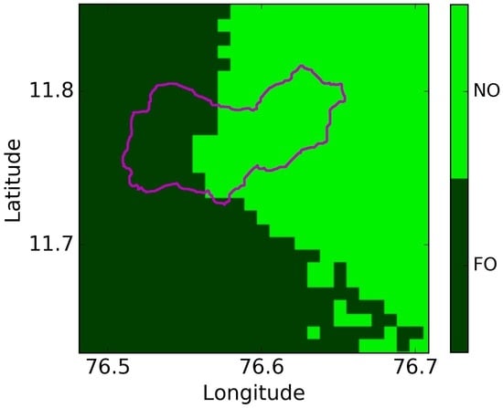
Figure 2.
Land-cover map for the study area as considered in the SMOS retrieval algorithm. “NO” is the nominal surface composed of bare soil and low vegetation and FO is for the forest land-cover.
2.2. Satellite Soil Moisture Datasets
For the active microwave, 30 RADARSAT-2 retrieved soil moisture maps were available over the study area based on the previous study from [30]. Details of the RADARSAT-2 maps are given in Table 1. They approximately cover the entire study area. Soil moisture was retrieved using the Cumulative Density Function (CDF) transformation at a spatial resolution of 20 m. The details of the CDF transformation along with the multi-scale validation of the retrieved soil moisture using measured soil moisture in 50 plots (1262 data) and SMOS soil moisture are given in [30]. Comparison of the retrieved soil moisture with the field data showed a Root Mean Squared Error (RMSE) ranging from 0.02 to 0.06 m/m for the majority of plots.

Table 1.
Details of the used RADARSAT-2 and SMOS soil moisture products. The up-scaled RADARSAT-2 SM is at a spatial resolution of 25 km.
SMOS (ESA Level 2 User Data Product v 551) soil moisture products for ascending and descending orbits are used for the passive microwave soil moisture data. The Discrete Global Grid (DGG) center lying inside the study area (ID number—3160498) is shown in the Figure 1. The soil moisture data are filtered for Radio Frequency Interferences (RFIs), data quality index (DQX) and Chi2 probability by excluding data associated with higher than the specified threshold of 10%, 0.05 m/m and 0.95 probability, respectively. This resulted in the exclusion of approximately 5% and 4% data due to the RFIs and DQX/Chi2, respectively. As presented in Table 1, 18 (10 for Descending and 8 for Ascending overpass) SMOS data were available concurrently with the RADARSAT-2 overpasses. Though the impact of RFI is sensibly different between ascending and descending overpasses, all data is used together to enhance the temporal availability. A good temporal behaviour between average RADARSAT-2 soil moisture and SMOS soil moisture was observed with an RMSE of approximately 0.06 m/m and Pearson’s correlation coefficient of approximately 0.9 [30].
3. Methodology
3.1. Merging Active and Passive Microwave Soil Moisture
This section contains the details of the Merging Active and Passive microwave Soil Moisture (MAPSM) algorithm. Figure 3 shows the spatial and temporal resolution of soil moisture products commonly available from active and passive microwave satellites. MAPSM attempts to combine the strength (high spatial resolution) of active microwave with the strength (high temporal resolution) of passive microwave to obtain a high spatio-temporal resolution soil moisture. Hereafter, the fine (active microwave) and coarse (passive microwave) data are represented respectively by an A and a P subscripts. The soil moisture at the fine scale at time t () can be expressed in terms of the most recent fine scale soil moisture (), the WCC at time t (), the fine scale spatial heterogeneity index (), the coarse scale soil moisture at time t () and the most recent coarse scale soil moisture () in the following manner:
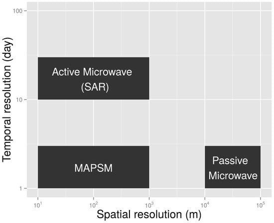
Figure 3.
Spatial and temporal resolution using a logarithmic scale for the active microwave (SAR), passive microwave (SMOS, SMAP) and MAPSM soil moisture products.
Here, the superscript i represents a RADARSAT-2 pixel within a SMOS pixel. The spatial variability is represented by two distinct components: () the time variant and () the time invariant. Note that the impact of the time interval between t and is analysed in the Results and discussion section. Equation (1) is applied independently to the each coarse scale (SMOS) grid point.
The time invariant describes the intrinsic surface heterogeneity. It takes into consideration the combined effect of three sources of spatial heterogeneity (soil texture, land cover and antenna footprint) present within a SMOS pixel and that can be computed as in [28]:
where, the overbar represents the average over space. is the mean antenna footprint, is the land cover value (1 for the nominal surfaces and 0 for the forest surfaces), is the clay fraction, which is used to account for soil texture variability. The mean antenna footprint for SMOS has a value of 1 in the center of SMOS pixel, and decreases with distance based on the antenna pattern. It has a value of around 0.5 at a distance of 20 km [5].
The time variant WCC combines two information that need to be identified: the direction (drying/wetting) and the magnitude of change. When the soil at coarse scale goes into wetting (or drying) state over time, it does not imply that all the fine scale pixels lying within will follow the same magnitude and direction of change. We propose to model the number of pixel following the opposite sign of change as a function of the magnitude of change at coarse scale by assuming a generalised logistic function in the following way:
where, is the fraction of pixel at fine scale undergoing wetting, is the fraction of pixel at fine scale undergoing drying, is the fraction of permanently wet pixel (e.g., perennial water bodies), is the fraction of permanently dry pixel (e.g., urban sealed surface), and k is a calibration coefficient that represents the heterogeneity of temporal change at fine scale. Theoretically, parameter k could vary between 0 to ∞. This impact of k on is shown in Figure 4 for three values (0, 70, 1000) of parameter k. The value of k equal to 0 means that irrespective of the magnitude and direction of change in the coarse scale soil moisture , a constant number of pixels undergo drying and wetting state. A very large value of k means that all the pixels will endure drying when soil is drying at coarse scale and vice versa. A value of k between 0–∞ ensures that even when no change in the coarse scale soil moisture is observed heterogeneity of the change at fine scale can be modeled.
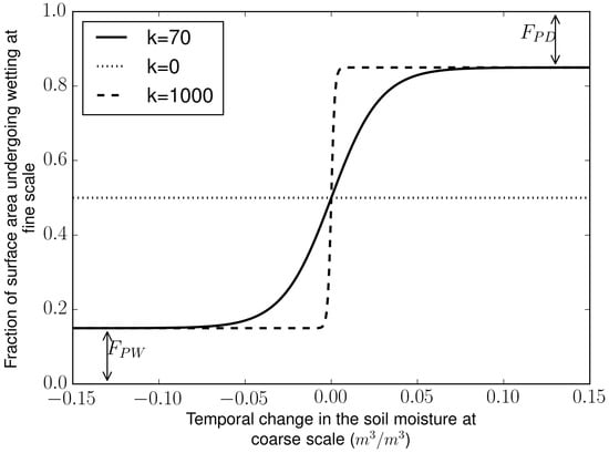
Figure 4.
Conceptual relationship between the fraction of surface undergoing wetting at fine scale () and the temporal change in the coarse scale soil moisture () for three different k values (0, 70, 1000).
The group of pixels that will undergo wetting is identified using the value of and the CDF of the relative soil moisture () defined in:
where, and are the minimum and maximum observed soil moisture for a pixel i. A schematic of the identification process of pixels undergoing wetting is shown in Figure 5. First, the CDF of the relative soil moisture (RSM) is computed. Then, a threshold of the relative soil moisture for the pixels undergoing drying/wetting () is computed by the following equation,
where, is the inverse CDF transformation of relative soil moisture. The pixels having a relative soil moisture less than will then undergo wetting and rest of the pixels will undergo drying.
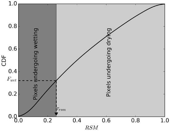
Figure 5.
Computation process of the threshold of the relative soil moisture () to identify pixels undergoing wetting based on the CDF of relative soil moisture and .
Two constraints for WCC are needed and can be written as follows:
- Mean of the over space is equal to one
- is 0 when the soil moisture is equal to the threshold of the relative soil moisture for the pixels undergoing drying/wetting ()
A linear model is proposed to model the as a function of
This equation can be solved for these two unknowns by using the two constraints mentioned in the Equations (7) and (8). The resulting solution is:
where, overbar represents the mean over space. Note that even though the relationship between and is assumed to be linear, the overall model is non-linear due to .
A schematic showing the behaviour of with respect to the is shown in Figure 6. Two scenarios are depicted: (i) assuming that soil is undergoing drying at the coarse scale; and (ii) the soil is undergoing wetting at the coarse scale. A threshold () of 0.7 and 0.3 was assume for the wetting and drying state respectively. The behaviour of one dry (assuming ) and one wet pixel (assuming ) is also shown in the figure. It can be seen that for both the drying and wetting state, the shows a value of 0 when is equal to the . Further, the pixels show different magnitude of change for drying and wetting events, e.g., a relatively wet pixel () show the magnitude of equal to 1.0 for wetting and 3.0 for drying. This is consistent with the fact that the equilibrium soil moisture at a given suction is greater in desorption (drying) than in absorption (wetting). Therefore, a pixel having higher water content in soil will have more capacity to loose water under a drying event and will have a less capacity to gain water under a wetting event. Similarly, a relatively dry pixels shows a higher capacity to gain water under a wetting event and lesser capacity to loose water under a drying event. The fact that the change of soil moisture depends not only on the previous state but also on its direction chows similarities with the phenomena of hysteresis observed in unsaturated soil [36], even though the process itself is not modelled in MAPSM.
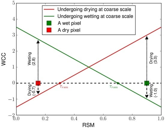
Figure 6.
Conceptual relationship showing the behaviour of with respect to the for a dry and a wet pixel.
Note that prior to merging the active and passive microwave soil moisture, they need to be compared and corrected for bias [19]. The quantile matching approach has been used in the literature to correct the bias [19,37]. It has been applied in the current study to adjust the SMOS soil moisture against the RADARSAT-2 soil moisture.
Figure 7 shows the schematic of the MAPSM algorithm. The step of the MAPSM model can be summarized as follows:
- correct the bias in SMOS soil moisture using the up-scaled RADARSAT-2 soil moisture,
- compute the bias corrected change in soil moisture at coarse scale ,
- calibrate the parameter k using the entire data,
- compute and from Equations (3) and (4) respectively,
- compute from Equation (6),
- compute from the Equation (10) for each RADARSAT-2 pixel and time t, and
- compute from the Equation (1) for each RADARSAT-2 pixel and time t.
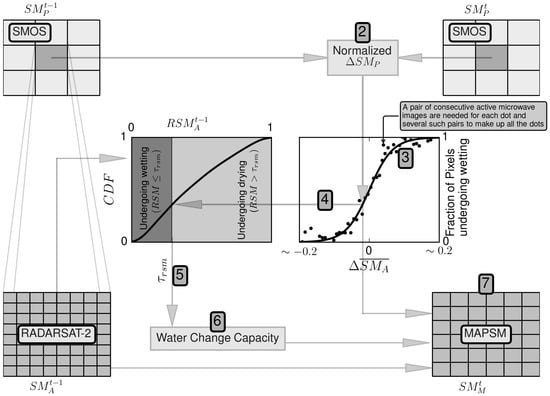
Figure 7.
Schematic of the MAPSM algorithm. Subscript A and P are for active and passive microwave, respectively. Numerals represent the step described in the text.
Steps 1–3 are required only once for a SMOS pixel, while the remaining steps need to be performed iteratively for each time step t.
3.2. Design of the Experiments
Four soil moisture disaggregation experiments are performed to evaluate the impact of the mismatch between soil moisture obtained from active and passive sensors at the coarse scale (P) spatial resolution. The description of these experiments is given Table 2. The arithmetic mean of the fine scale soil moisture () is assumed to be representative of the coarse scale soil moisture () in the experiments denoted by an “F” as first letter (experiments No. 1 and 2 in the table). And, first letter is denoted by “C” when the actual coarse scale soil moisture is used (experiments No. 3 and 4 in the table). Two scenarios of estimation of are considered:
- equal to one. In this case the change in the coarse scale soil moisture is equally redistributed across the fine scale pixels (F-Linear and C-Linear).
- computed using the calibrated k parameter (F-Cal and C-Cal). The k is calibrated using the time series of soil moisture from active microwave at fine scale.
Table 2.
Description of the soil moisture disaggregation experiments.
3.3. Validation Strategy
Validation strategy for the MAPSM model is shown in Figure 8. MAPSM is applied when data from both RADARSAT-2 and SMOS are available, but without using the . Then, the model is tested by comparing the computed with the RADARSAT-2 retrieved soil moisture () at the same date. Performance of the model output is assessed in terms of correlation coefficient and RMSE.
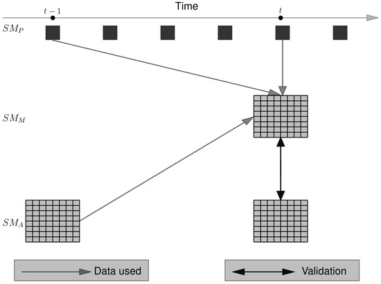
Figure 8.
Validation strategy for the MAPSM model. Subscript A, P and M stands for the active microwave, passive microwave and MAPSM respectively.
4. Results
4.1. Bias Correction at Coarse Scale
The comparison of soil moisture at coarse scale from the two sensors showed a negligible bias, however there was a significant difference in the range i.e., soil moisture is varying from approximately 0.10 to 0.21 m/m for RADARSAT-2 while it is varying from 0.01 to 0.3 m/m for SMOS. This difference in range is corrected using the quantile matching. A total of 18 soil moisture data are available concurrently from SMOS and RADARSAT-2 data (see Table 1). Twelve data are used for the calibration and the remaining six are used for the validation. The comparison for the calibration and validation period is shown in the Figure 9. The RMSE was 0.021 m/m and 0.018 m/m for the calibration and validation period, respectively, which is much lower when compared to the uncorrected values of approximately 0.06 m/m. After correction, the RMSE was quite low given the fact that SMOS and RADARSAT-2 apperate at different frequencies and technologies (passive L-Band and active C-Band).
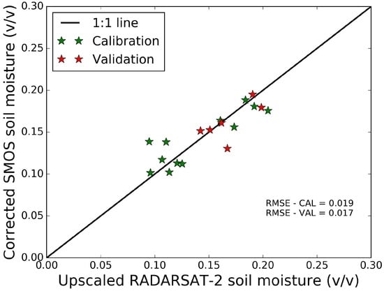
Figure 9.
Comparison of the bias corrected SMOS soil moisture with upscaled RADARSAT-2 soil moisture for the calibration and validation period.
4.2. Estimation of Parameter k
Since there is no major water body or major urban area in the study area, and are assumed to be equal to 0. Parameter k is computed by least square fitting the objective function in terms of RMSE using the soil moisture retrieved from the RADARSAT-2. To avoid the effect of discrepancy in the soil moisture from two different sensors, the soil moisture at coarse scale is computed by upscaling the fine scale soil moisture. Since a pair of consecutive RADARSAT-2 images are required to compute , 29 data values are available for the estimation of parameter k. Out of 29 data values, 18 are used for the calibration and the remaining 11 are used for the validation. The k parameter is estimated at the spatial resolution varying from 20 m to 2000 m. No significant difference is observed in the RMSE for the calibration and validation periods at all the studied spatial resolutions. As an example, the relationship at a spatial resolution of 1000 m along with the fitted sigmoid model is shown in the Figure 10. The estimated value of k is found to be 96.8 with a standard error of 12.98 at a spatial resolution of 1000 m. Based on the result obtained in Figure 10, it can be inferred that not all fine scale pixels follow the same sign of change (drying/wetting) observed at the coarse scale. The fraction of area is dependent on the magnitude of change at the coarse scale. A higher magnitude shows a larger fraction.
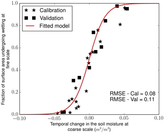
Figure 10.
Computed and observed (fraction of surface area undergoing wetting at fine scale) at a spatial resolution of 1000 m from the retrieved RADARSAT-2 soil moisture as a function of the change in the soil moisture at coarse scale.
The behaviour of the k parameter with respect to the spatial resolution is shown in Figure 11. Parameter k showed an exponential behaviour with the spatial resolution. The fitted exponential curve is also shown in the figure. Parameter k was also estimated using the soil moisture data measured in the field plots. The value of k for the field data is found to be 31.38 with a standard error of 3.27, which is close to the value obtained using RADARSAT-2 soil moisture at a spatial resolution of 50 m (approximate spatial resolution of the field plots).
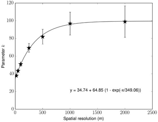
Figure 11.
Observed variation of the parameter k with the spatial resolution. Fitted exponential curve is also shown.
5. Discussion
5.1. Validation Using RADARSAT-2 SM
First the coherency of the soil moisture spatial patterns at fine scale is evaluated by analysing the auto-correlation between two consecutive images obtained from RADARSAT-2, which is shown in Figure 12. The figure shows also the auto-correlation at a spatial resolution of 1000 m. The behaviour of the auto-correlation is observed to be similar at the spatial resolution varying from 20 m to 2000 m, with the difference in the relative magnitude of the auto-correlation function (not shown here). In most of the cases the auto-correlation is observed to be significant (higher than 0.368, ). The auto-correlation is observed to be insignificant when the gap between two consecutive image is higher than 24 days (marked by 1, 2, 4 and 7 in the figure) or when there is a change in the cropping season (marked by 3, 5, 6 and 8 in the figure). The impact of the change in soil roughness from farming practices could be a possible reason for the low correlation during change of cropping season. It can be inferred that the use of a time invariant spatial variability over a longer period as in Blöschl et al. [13] is insufficient, and that a time variant spatial variability is required. Here it is estimated by using the recently available active microwave soil moisture data. In the case of a change in the cropping season, once a RADARSAT-2 image becomes available, it can be used to obtain the merged soil moisture for the remaining cropping season, and hence only for a short (less than the temporal resolution length) duration the model may not work. A total of 20 RADARSAT-2 images are found to be suitable and are selected for the F-Linear and F-Cal experiments. Out of these 20 images, only 8 images have the SMOS and RADARSAT-2 soil moisture concurrently available. This gives 7 pair of images suitable for the C-Linear and C-Cal experiments.
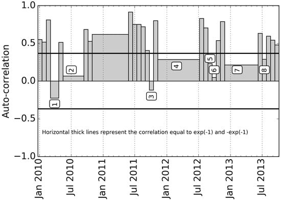
Figure 12.
Auto-correlation among two consecutive SM images of RADARSAT-2 at a spatial resolution of 1000 m.
For each of the experiments, MAPSM is run at the spatial resolution of 20 m, 50 m, 100 m, 250 m, 500 m and 1000 m. RMSE is computed for each of these experiments for every spatial resolution and mean of the RMSE is used to analyse the effect of the spatial resolution on the retrieval accuracy of MAPSM at different spatial resolutions. The mean RMSE for the spatial resolution of 20 m, 50 m, 100 m, 250 m, 500 m and 1000 m is shown in the Figure 13 for all the four experiments. For all the experiments, RMSE showed a monotonically decreasing behaviour. RMSE showed a relatively stable behaviour at higher resolution than 250 m. Merlin et al. [38] assessed the relation between spatial resolution and RMSE in the Dispatch algorithm and found same behavior as MAPSM. The application of Dispatch over the current site was hampered by cloud cover. There was difference in the mean RMSE of F and C experiments for all the spatial resolution tested, which showed the impact of difference in the soil moisture retrieved using active and passive microwave satellites. In the current study, the active and passive satellites have different (C for active and L for passive) bands. Use of a similar band for both the active and passive microwave might bring them closer. Das et al. [25] showed lower RMSE (0.01–0.02 m/m) values when using simultaneous radar and radiometer L-Band acquisition. In the current status of existing space platforms it is not possible to test such exercise. Since, there is no significant difference in the mean RMSE obtained at a spatial resolution of 500 m and 1000 m from MAPSM, henceforth only the results for the spatial resolution of 500 m are presented.
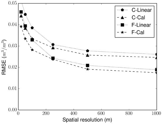
Figure 13.
Behaviour of the observed mean RMSE for all the four experiments of MAPSM with the spatial resolution.
The comparison of the merged soil moisture with the RADARSAT-2 retrieved soil moisture at a spatial resolution of 500 m for the F-Linear experiment is shown in the Figure 14. The merged soil moisture showed a good behaviour with the RADARSAT-2 retrieved soil moisture having a median (over time) RMSE of 0.023 m/m and a median (over time) correlation of 0.68. The comparison for the F-Cal experiment is shown in the Figure 15. The median (over time) of the RMSE and correlation for this experiment is found to be 0.019 m/m and 0.66, respectively. The F-Cal approach is found to be moderately superior to the F-Linear in terms of RMSE, while correlation is observed to be nearly same. Availability of only 20 images hinder the identification of the superiority of one experiments over another in terms of seasonality. Since mean of the fine scale soil moisture is assumed as the proxy of coarse scale soil moisture for these two experiments, the bias is found to be 0.
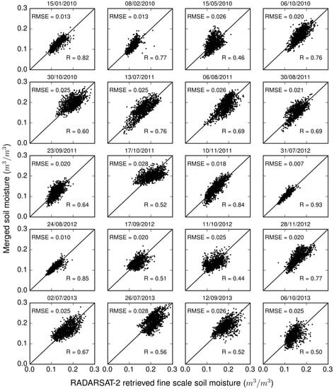
Figure 14.
Comparison of the merged soil moisture with the RADARSAT-2 retrieved soil moisture at a spatial resolution of 500 m for the F-Linear experiment.
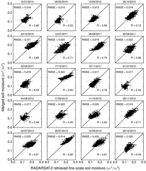
Figure 15.
Comparison of the merged soil moisture with the RADARSAT-2 retrieved soil moisture at a spatial resolution of 500 m for the F-Cal experiment.
The comparison of the observed and estimated from F-Linear and F-Cal experiments is shown in the Figure 16. F-Linear experiment fails to capture the percentage of pixels undergoing drying or wetting state, which is expected. The fraction of pixels undergoing drying or wetting state are captured quite well by the F-Cal experiment. Though the difference in terms of RMSE is lesser, the improvement in terms of capturing the change in the state of pixels is significant.
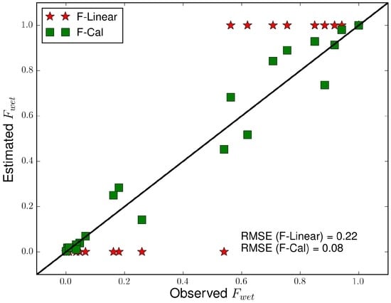
Figure 16.
Comparison of the observed and estimated for the F-Linear and F-Cal experiments at a spatial resolution of 500 m.
Comparison of the merged soil moisture with the RADARSAT-2 retrieved soil moisture at a spatial resolution of 500 m for the C-Linear experiment is shown in the Figure 17. The comparison for the C-Cal experiment is shown in the Figure 18. The median (over time) of the RMSE is observed to be approximately same for both the experiment having a value of 0.026 m/m. The median (over time) of correlation is also observed to be approximately same having a value of 0.63 and 0.70 for the C-Linear and C-Cal experiments, respectively. Since MAPSM conserves the mean irrespective of the value of parameter k, the same bias is observed in both the experiments. Since, the has the lower limit of 0 and upper limit of 1, the model output is bounded by observed and , as observed in the results presented in two subfigures of the Figure 18.
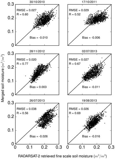
Figure 17.
Comparison of the merged soil moisture with the RADARSAT-2 retrieved soil moisture at a spatial resolution of 500 m for the C-Linear experiment.
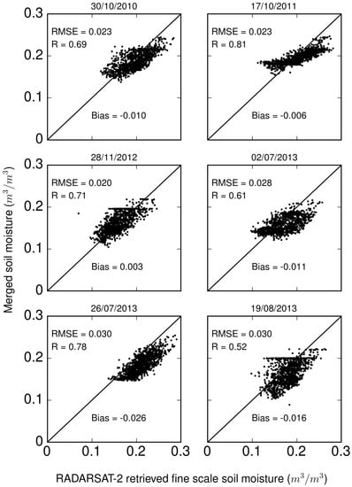
Figure 18.
Comparison of the merged soil moisture with the RADARSAT-2 retrieved soil moisture at a spatial resolution of 500 m for the C-Cal experiment.
The comparison of the observed and estimated from C-Linear and C-Cal experiments is shown in the Figure 19. F-Linear experiment fails to capture the percentage of pixels undergoing drying or wetting state. They are well captured in the C-Cal experiment. This suggests that though there is minor improvement in the RMSE in the C-Cal experiment over the C-Linear experiment, the improvement in terms of capturing the dynamics of the pixels state is significant. Among the C and F experiments, overall the Cal showed similar to moderate improvement of RMSE, and a significant improvement of .
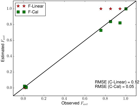
Figure 19.
Comparison of the observed and estimated for the C-Linear and C-Cal experiments.
Figure 20 shows the spatial distribution of the observed soil moisture along with the that of C-Linear and C-Cal experiments for two events (19 June 2011–13 July 2011 and 29 September 2011–17 October 2011). Both the experiments are able to clearly identify the wet valley region. C-Cal showed relatively smoother spatial behaviour compared to C-Linear for the two events. Since the first event is a systematic dry event, C-Linear showed a relatively better spatial distribution compared to the observed spatial distribution, while for the second event better performance is shown by the C-Cal experiments. Comparison of the spatial distribution for the F-Linear and F-Cal experiment for the two events (6 October 2011–30 October 2011 and 2 July 2013–26 July 2013) with the observed data is shown in the Figure 21. Here also Cal experiments showed smoother spatial behaviour as was the case for F experiments. While comparing to the observed spatial distribution, a relatively better comparison is observed in the case of first event than the second event. This is because the bias was relatively low for the first event (19 June 2011–13 July 2011).
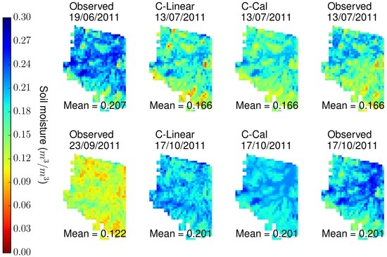
Figure 20.
Comparison of the spatial distribution for the observed and MAPSM soil moisture at a spatial resolution of 500 m for the C-Cal and C-Linear experiments for two events. Observed spatial distribution on 19 June 2011 is used to retrieve the soil moisture for 13 July 2011 and 23 September 2011 is used for 17 October 2011.
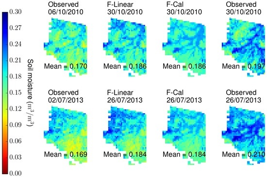
Figure 21.
Comparison of the spatial distribution for the observed and MAPSM soil moisture at a spatial resolution of 500 m for the F-Cal and F-Linear experiments. Observed spatial distribution on 6 October 2010 is used to retrieve the soil moisture for 30 October 2010 and 2 July 2013 is used for the 26 July 2013.
5.2. Validation Using Field Measured SM
The MAPSM soil moisture is compared with the averaged field measured soil moisture at the spatial resolution of 500 m. The number of plots falling into the grids varies from 1 to 3. The comparison for the entire study period is presented in the Figure 22. MAPSM showed a reasonable estimation of soil moisture at a spatial resolution of 500 m, with an RMSE of 0.069 m/m and a correlation coefficient of 0.76. A slight overestimation (0.03 m/m for the lower range of soil moisture, and an important underestimation for the higher range of soil moisture is observed. In this case the MAPSM data presents a plateau at relatively low soil moistures (0.22), this may be due to saturation effect observed in the SAR retrievals [39] and the propagation of this saturation to SMOS data by the CDF matching.
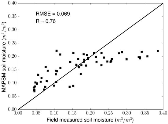
Figure 22.
Comparison of the MAPSM soil moisture with the field measured soil moisture at the spatial resolution of 500 m for the entire study period.
6. Conclusions
In the current paper, an algorithm for Merging Active and Passive microwave Soil Moisture (MAPSM) is developed. The algorithm merges the soil moisture retrieved from active (fine spatial scale and coarse temporal resolution) and passive (coarse spatial scale and fine temporal resolution) microwave satellites. The algorithm relies on temporally transforming the fine scale information based on the innovative concept of water change capacity. This concept expresses the magnitude at which the soil at fine scale is impacted by a soil moisture change at the coarser scale.
From the RADARSAT-2 retrieved and field measured soil moisture data, it was observed that when the soil moisture at a coarse scale undergoes wetting, not all the pixels at fine scale will endure wetting and vice-versa. The fraction of pixels following the similar trend as of coarse scale is observed to be dependent on the magnitude of change at the coarse scale. A sigmoid curve based model is found to be suitable to model this behaviour. This model is parsimonious, it requires only one calibration parameter. The effect of the spatial resolution on this parameter is also studied.
The scale parameter (k) in MAPSM model showed an exponential behaviour with the spatial resolution, suggesting the applicability of MAPSM over a wide range of spatial resolutions. A value of k = 80 was obtained for a spatial resolution of 500 m for the Berambadi watershed. MAPSM model is applied and validated using the retrieved soil moisture maps from the RADARSAT-2 data for different spatial resolutions. The model is able to estimate the fine scale soil moisture quite reasonably. A mean RMSE of around 0.02 m/m is observed when there was no difference in the soil moisture from active and passive microwave, while it increased to 0.03 m/m when differences were present. As the model is parsimonious, it has the potential to be applied globally in merging soil moisture from active and passive microwave satellites. A potential shortcoming of the MAPSM model is that it cannot model the impact of forcing if applied only over a fraction of area e.g., if irrigation is applied over only a small portion of the watershed. However, as after some time (24 days in the case of RADARSAT-2) a new spatial information would be available, the impact of the irrigation is mitigated afterwards. Work is in progress to apply the MAPSM methodology to Sentinel-1 and RISAT missions. RISAT presents a low revisit frequencies which increases the interest for MAPSM. It is the case also for Sentinel-1 mission outside the European continent. The algorithm can also be used to merge SMOS / SMAP and Sentinel-1 data. Nevertheless these applications will need specific updates of the algorithm to take into account for example the angle sampling and resolution of Sentinel-1 and RISAT data or the mismatch between SMOS and SMAP.
Acknowledgments
This research work was funded by TOSCA (Terre Océan Surfaces Continentales et Atmosphère) CNES program. The SMOSL2 data provided by European Space Agency is duly acknowledged. RADARSAT-2 data procured under RISAT-1 (Radar Imaging SATellite) utilization programme of ISRO is gratefully acknowledged. The authors are also thankful for partial financial support received under the IISc-STC project (ISTC/CCE/MS/214). This work was also supported by the VIGISAT-CLS project which provided the RADARSAT-2 satellite dataset from 2012 to 2014. The funding from CEFIPRA project 4700-W1 and ISRO0198 for the salary of project personnel, instruments and field studies is also acknowledged. The authors would like to thank the filed team and the help provided during the field campaigns by the farmers.
Author Contributions
Sat Kumar Tomer and Ahmad Al Bitar elaborated the algorithm and provided the first draft of the paper; Sat Kumar Tomer made the RadarSat2 and MAPSM analysis; Ahmad Al Bitar and Yann Kerr extracted and provided expertise on the SMOS data; Muddu Sekhar provided the field data and updates to the methodology; Mehrez Zribi and Soumya Bandyopadhyay provided expertise on radar data. All authors contributed to the writting and review of the final version.
Conflicts of Interest
The authors declare no conflict of interest.
Abbreviations
The following abbreviations are used in this manuscript:
| CDF | Cumulative Density Function |
| CF | Clay Fraction |
| CNES | Centre National d’Etudes Spatiales |
| DQX | data quality index |
| ESA | European Space Agency |
| LAI | Leaf Area Index |
| LC | Land Cover |
| LDAS | Land Data Assimilation System |
| LST | Land Surface Temperature |
| MAF | Mean antenna footprint |
| MAPSM | Merging Active and Passive microwave Soil Moisture |
| RADARSAT-2 | RADAR SATellite-2 |
| RFI | Radio Frequency Interference |
| RISAT | Radar Imaging SATellite |
| RMSE | Root Mean Squared Error |
| RSM | Relative Soil Moisture |
| SAR | Synthetic Aperture Radar |
| SH | Spatial heterogeneity index |
| SM | Soil Moisture |
| SMAP | Soil Moisture Active Passive |
| SMOS | Soil Moisture and Ocean Salinity |
| ST | Soil Texture |
| VWC | Vegetation Water Content |
| WCC | Water Change Capacity |
References
- Lakshmi, V. Remote Sensing of Soil Moisture. ISRN Soil Sci. 2013, 2013. [Google Scholar] [CrossRef]
- Al-Yaari, A.; Wigneron, J.P.; Ducharne, A.; Kerr, Y.; De Rosnay, P.; De Jeu, R.; Govind, A.; Al Bitar, A.; Albergel, C.; Munoz-Sabater, J.; et al. Global-scale evaluation of two satellite-based passive microwave soil moisture datasets (SMOS and AMSR-E) with respect to Land Data Assimilation System estimates. Remote Sens. Environ. 2014, 149, 181–195. [Google Scholar] [CrossRef]
- Chaurasia, S.; Tung, D.T.; Thapliyal, P.; Joshi, P. Assessment of the AMSR-E soil moisture product over India. Int. J. Remote Sens. 2011, 32, 7955–7970. [Google Scholar] [CrossRef]
- Liu, Y.; Dorigo, W.; Parinussa, R.; De Jeu, R.; Wagner, W.; McCabe, M.; Evans, J.; Van Dijk, A. Trend-preserving blending of passive and active microwave soil moisture retrievals. Remote Sens. Environ. 2012, 123, 280–297. [Google Scholar] [CrossRef]
- Kerr, Y.H.; Waldteufel, P.; Richaume, P.; Wigneron, J.P.; Ferrazzoli, P.; Mahmoodi, A.; Al Bitar, A.; Cabot, F.; Gruhier, C.; Juglea, S.E.; et al. The SMOS soil moisture retrieval algorithm. IEEE Trans. Geosci. Remote Sens. 2012, 50, 1384–1403. [Google Scholar] [CrossRef]
- Brocca, L.; Hasenauer, S.; Lacava, T.; Melone, F.; Moramarco, T.; Wagner, W.; Dorigo, W.; Matgen, P.; Martínez-Fernández, J.; Llorens, P.; et al. Soil moisture estimation through ASCAT and AMSR-E sensors: An intercomparison and validation study across Europe. Remote Sens. Environ. 2011, 115, 3390–3408. [Google Scholar] [CrossRef]
- Albergel, C.; de Rosnay, P.; Gruhier, C.; Muñoz-Sabater, J.; Hasenauer, S.; Isaksen, L.; Kerr, Y.; Wagner, W. Evaluation of remotely sensed and modelled soil moisture products using global ground-based in situ observations. Remote Sens. Environ. 2012, 118, 215–226. [Google Scholar] [CrossRef]
- Moran, S.; Hymer, D.; Qi, J.; Sano, E. Soil moisture evaluation using multi-temporal synthetic aperture radar (SAR) in semiarid rangeland. Agric. For. Meteorol. 2000, 105, 69–80. [Google Scholar] [CrossRef]
- Quesney, A.; Le Hégarat-Mascle, S.; Taconet, O.; Vidal-Madjar, D.; Wigneron, J.; Loumagne, C.; Normand, M. Estimation of watershed soil moisture index from ERS/SAR data. Remote Sens. Environ. 2000, 72, 290–303. [Google Scholar] [CrossRef]
- Oldak, A.; Jackson, T.; Starks, P.; Elliott, R. Mapping near-surface soil moisture on regional scale using ERS-2 SAR data. Int. J. Remote Sens. 2003, 24, 4579–4598. [Google Scholar] [CrossRef]
- Zribi, M.; Kotti, F.; Amri, R.; Wagner, W.; Shabou, M.; Lili-Chabaane, Z.; Baghdadi, N. Soil moisture mapping in a semiarid region, based on ASAR/Wide Swath satellite data. Water Resour. Res. 2014, 50, 823–835. [Google Scholar] [CrossRef]
- Merlin, O.; Walker, J.P.; Chehbouni, A.; Kerr, Y. Towards deterministic downscaling of SMOS soil moisture using MODIS derived soil evaporative efficiency. Remote Sens. Environ. 2008, 112, 3935–3946. [Google Scholar] [CrossRef]
- Blöschl, G.; Komma, J.; Hasenauer, S. Hydrological downscaling of soil moisture. In Final Report to H-Sat (Hydrology Satellite Application Facility) via the Austrian Central Institute for meteorology and Geodynamics (ZAMG); Vienna University of Technology: Vienna, Austria, 2009. [Google Scholar]
- Piles, M.; Camps, A.; Vall-Llossera, M.; Corbella, I.; Panciera, R.; Rudiger, C.; Kerr, Y.H.; Walker, J. Downscaling SMOS-derived soil moisture using MODIS visible/infrared data. IEEE Trans. Geosci. Remote Sens. 2011, 49, 3156–3166. [Google Scholar] [CrossRef]
- Merlin, O.; Rüdiger, C.; Al Bitar, A.; Richaume, P.; Walker, J.P.; Kerr, Y.H. Disaggregation of SMOS soil moisture in Southeastern Australia. IEEE Trans. Geosci. Remote Sens. 2012, 50, 1556–1571. [Google Scholar] [CrossRef]
- Nagarajan, K.; Judge, J. Spatial scaling and variability of soil moisture over heterogeneous land cover and dynamic vegetation conditions. IEEE Geosci. Remote Sens. Lett. 2013, 10, 880–884. [Google Scholar] [CrossRef]
- Molero, B.; Merlin, O.; Malbéteau, Y.; Al Bitar, A.; Cabot, F.; Stefan, V.; Kerr, Y.; Bacon, S.; Cosh, M.H.; Bindlish, R. SMOS disaggregated soil moisture product at 1km resolution: Processor overview and first validation results. Remote Sens. Environ. 2016, 180, 361–376. [Google Scholar] [CrossRef]
- Reichle, R.H.; Entekhabi, D.; McLaughlin, D.B. Downscaling of radio brightness measurements for soil moisture estimation: A four-dimensional variational data assimilation approach. Water Resour. Res. 2001, 37, 2353–2364. [Google Scholar] [CrossRef]
- Liu, Y.; Parinussa, R.; Dorigo, W.; De Jeu, R.; Wagner, W.; Van Dijk, A.; McCabe, M.; Evans, J. Developing an improved soil moisture dataset by blending passive and active microwave satellite-based retrievals. Hydrol. Earth Syst. Sci. 2011, 15, 425–436. [Google Scholar] [CrossRef]
- Kim, G.; Barros, A.P. Downscaling of remotely sensed soil moisture with a modified fractal interpolation method using contraction mapping and ancillary data. Remote Sens. Environ. 2002, 83, 400–413. [Google Scholar] [CrossRef]
- Balsamo, G.; Mahfouf, J.; Bélair, S.; Deblonde, G. A land data assimilation system for soil moisture and temperature: An information content study. J. Hydrometeorol. 2007, 8, 1225–1242. [Google Scholar] [CrossRef]
- Carrera, M.L.; Bélair, S.; Bilodeau, B. The Canadian Land Data Assimilation System (CaLDAS): Description and Synthetic Evaluation Study. J. Hydrometeorol. 2015. [Google Scholar] [CrossRef]
- Piles, M.; Entekhabi, D.; Camps, A. A change detection algorithm for retrieving high-resolution soil moisture from SMAP radar and radiometer observations. IEEE Trans. Geosci. Remote Sens. 2009, 47, 4125–4131. [Google Scholar] [CrossRef]
- Das, N.N.; Entekhabi, D.; Njoku, E.G. An algorithm for merging SMAP radiometer and radar data for high-resolution soil-moisture retrieval. IEEE Trans. Geosci. Remote Sens. 2011, 49, 1504–1512. [Google Scholar] [CrossRef]
- Das, N.N.; Entekhabi, D.; Njoku, E.G.; Shi, J.J.C.; Johnson, J.T.; Colliander, A. Tests of the SMAP combined radar and radiometer algorithm using airborne field campaign observations and simulated data. IEEE Trans. Geosci. Remote Sens. 2014, 52, 2018–2028. [Google Scholar] [CrossRef]
- Kerr, Y.H.; Waldteufel, P.; Wigneron, J.P.; Martinuzzi, J.; Font, J.; Berger, M. Soil moisture retrieval from space: The Soil Moisture and Ocean Salinity (SMOS) mission. IEEE Trans. Geosci. Remote Sens. 2001, 39, 1729–1735. [Google Scholar] [CrossRef]
- Kerr, Y.H.; Al-Yaari, A.; Rodriguez-Fernandez, N.; Parrens, M.; Molero, B.; Leroux, D.; Bircher, S.; Mahmoodi, A.; Mialon, A.; Richaume, P.; et al. Overview of SMOS performance in terms of global soil moisture monitoring after six years in operation. Remote Sens. Environ. 2016, 180, 40–63. [Google Scholar] [CrossRef]
- Al Bitar, A.; Leroux, D.; Kerr, Y.H.; Merlin, O.; Richaume, P.; Sahoo, A.; Wood, E.F. Evaluation of SMOS soil moisture products over continental US using the SCAN/SNOTEL network. IEEE Trans. Geosci. Remote Sens. 2012, 50, 1572–1586. [Google Scholar] [CrossRef]
- Leroux, D.J.; Kerr, Y.H.; Al Bitar, A.; Bindlish, R.; Jackson, T.J.; Berthelot, B.; Portet, G. Comparison between SMOS, VUA, ASCAT, and ECMWF soil moisture products over four watersheds in US. IEEE Trans. Geosci. Remote Sens. 2014, 52, 1562–1571. [Google Scholar] [CrossRef]
- Tomer, S.K.; Al Bitar, A.; Sekhar, M.; Zribi, M.; Bandyopadhyay, S.; Sreelash, K.; Sharma, A.; Corgne, S.; Kerr, Y. Retrieval and multi-scale validation of soil moisture from multi-temporal SAR data in a semi-arid tropical region. Remote Sens. 2015, 7, 8128–8153. [Google Scholar] [CrossRef]
- Morena, L.; James, K.; Beck, J. An introduction to the RADARSAT-2 mission. Can. J. Remote Sens. 2004, 30, 221–234. [Google Scholar] [CrossRef]
- Kottek, M.; Grieser, J.; Beck, C.; Rudolf, B.; Rubel, F. World map of the Köppen-Geiger climate classification updated. Meteorol. Z. 2006, 15, 259–263. [Google Scholar] [CrossRef]
- Karnataka State Remote Sensing Application Centre. Report on State Natural Resources Information System; Technical Report; Department of IT, BT and S & T, Government of Karnataka: Bangalore, India, 2007.
- Sreelash, K.; Sekhar, M.; Ruiz, L.; Tomer, S.; Guérif, M.; Buis, S.; Durand, P.; Gascuel-Odoux, C. Parameter estimation of a two-horizon soil profile by combining crop canopy and surface soil moisture observations using GLUE. J. Hydrol. 2012, 456, 57–67. [Google Scholar] [CrossRef]
- Sreelash, K.; Sekhar, M.; Ruiz, L.; Buis, S.; Bandyopadhyay, S. Improved modeling of groundwater recharge in agricultural watersheds using a combination of crop model and remote sensing. J. Indian Inst. Sci. 2013, 93, 189–207. [Google Scholar]
- Haines, W.B. Studies in the physical properties of soil. V. The hysteresis effect in capillary properties, and the modes of moisture distribution associated therewith. J. Agric. Sci. 1930, 20, 97–116. [Google Scholar] [CrossRef]
- Reichle, R.H.; Koster, R.D. Bias reduction in short records of satellite soil moisture. Geophys. Res. Lett. 2004, 31. [Google Scholar] [CrossRef]
- Merlin, O.; Al Bitar, A.; Walker, J.P.; Kerr, Y. A sequential model for disaggregating near-surface soil moisture observations using multi-resolution thermal sensors. Remote Sens. Environ. 2009, 113, 2275–2284. [Google Scholar] [CrossRef]
- Baghdadi, N.; Cerdan, O.; Zribi, M.; Auzet, V.; Darboux, F.; El Hajj, M.; Bou Kheir, R. Operational performance of current synthetic aperture radar sensors in mapping soil surface characteristics in agricultural environments: Application to hydrological and erosion modelling. Hydrol. Process. 2008, 22, 9–20. [Google Scholar] [CrossRef]
© 2016 by the authors; licensee MDPI, Basel, Switzerland. This article is an open access article distributed under the terms and conditions of the Creative Commons Attribution (CC-BY) license (http://creativecommons.org/licenses/by/4.0/).