
Flow Routing for Delineating Supraglacial Meltwater Channel Networks


Abstract
:
1. Introduction
2. Materials and Methods
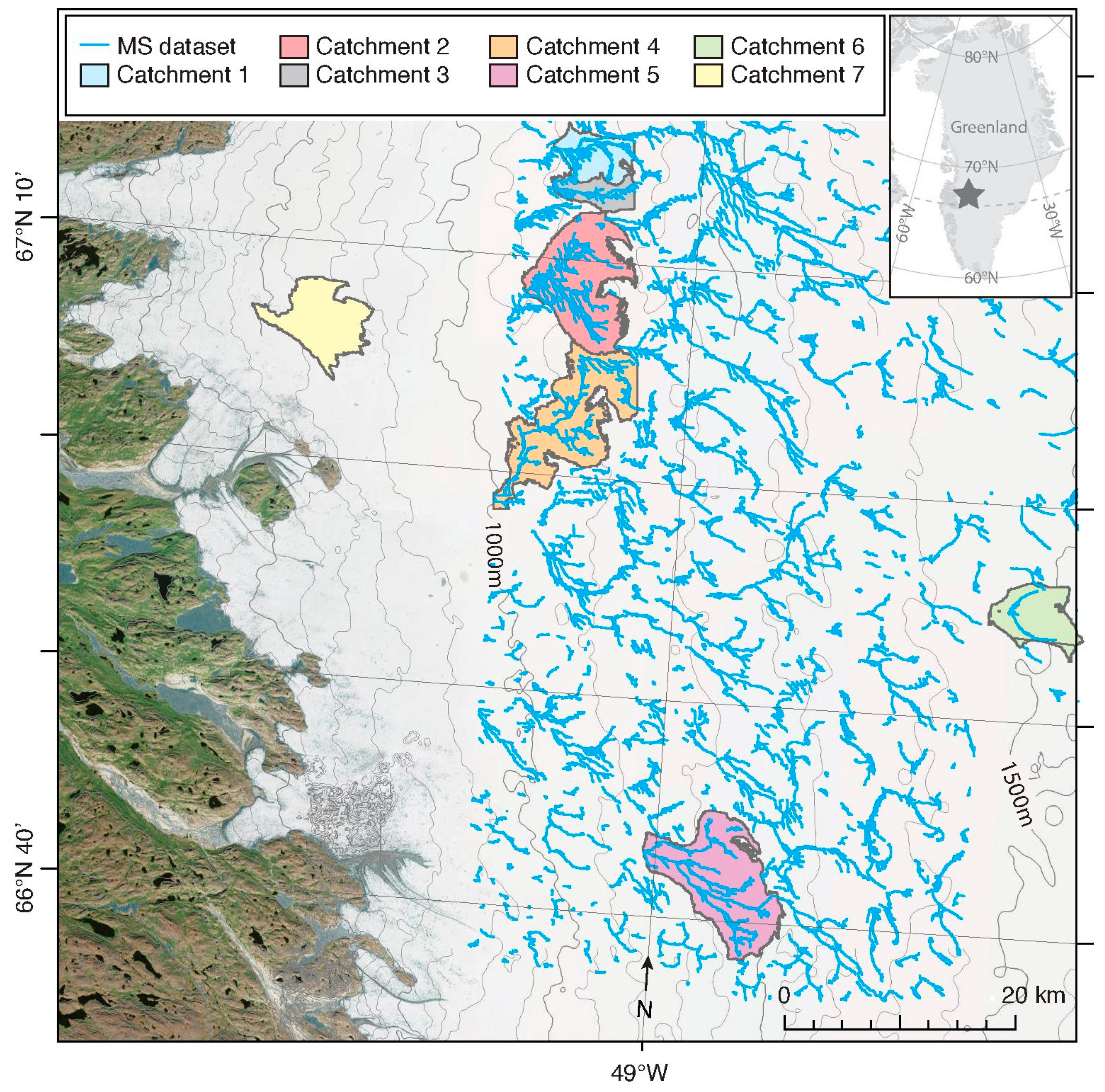
2.1. Datasets and Study Area
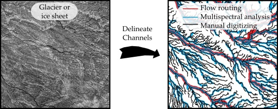
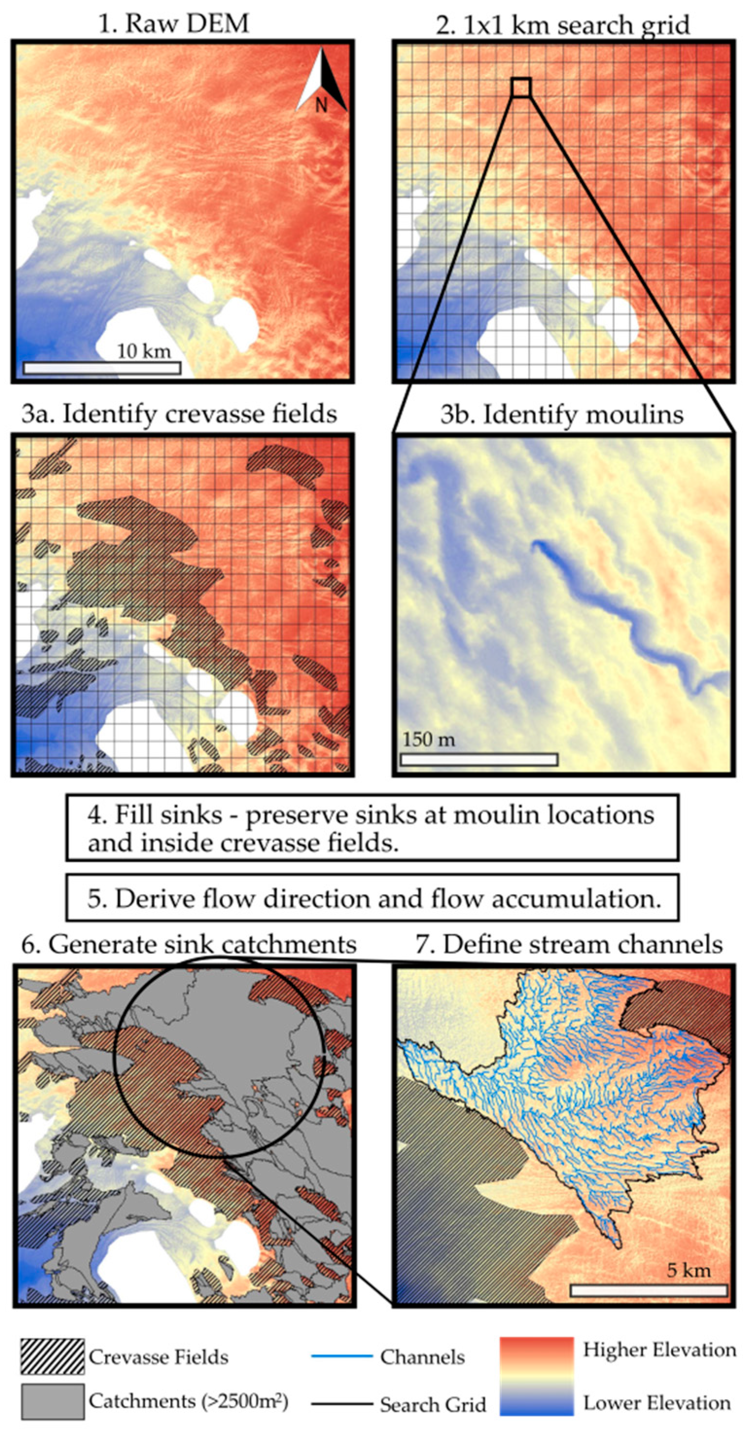
2.2. Channel Network Extraction
2.3. Channel Initiation Threshold
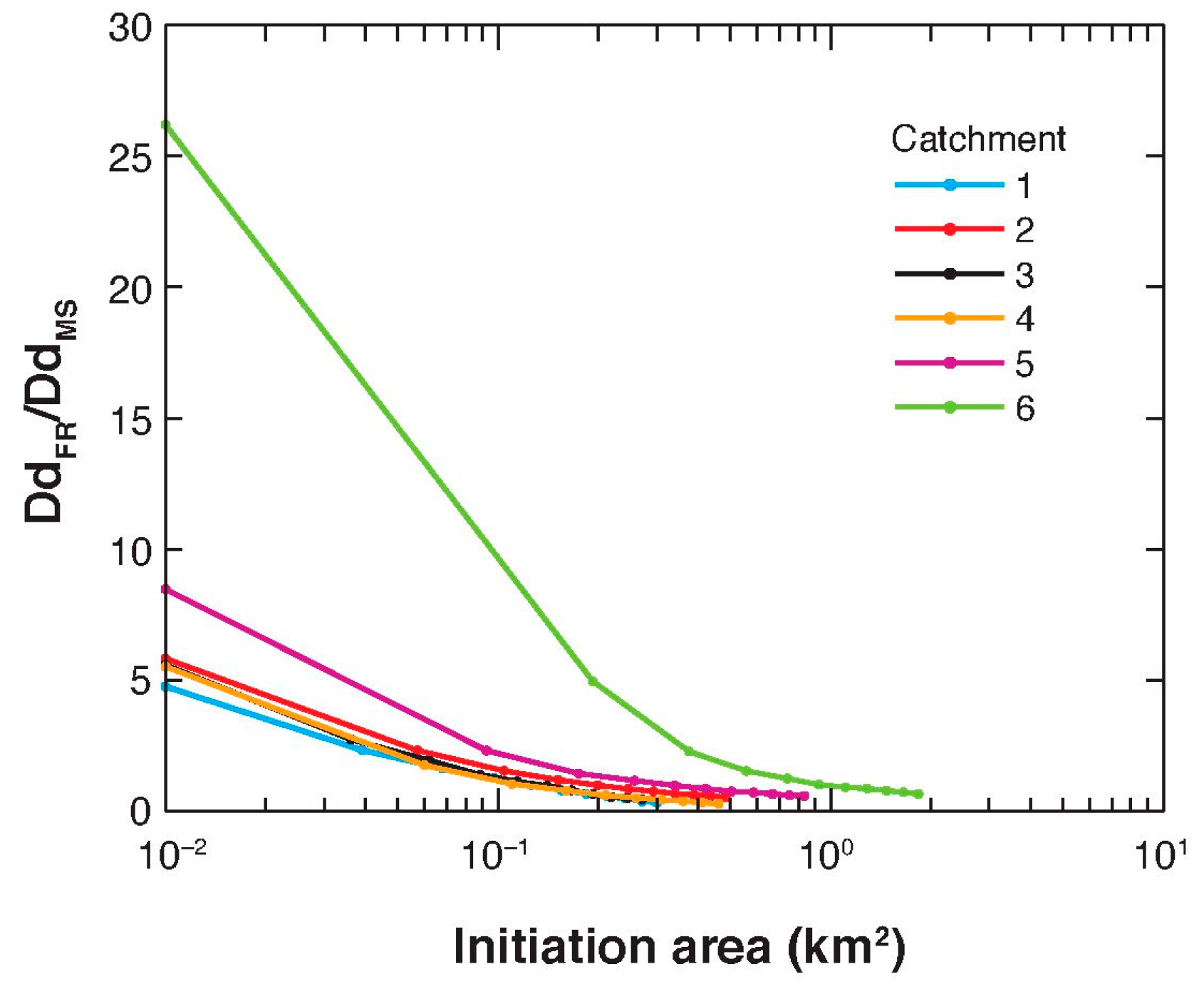
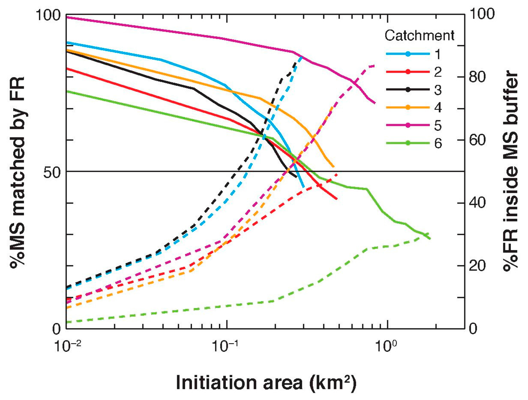
2.4. Quantification of Discrepancy between Datasets
3. Results
3.1. Comparison between Flow Routing and Multispectral Datasets
3.1.1. Moulin Identification
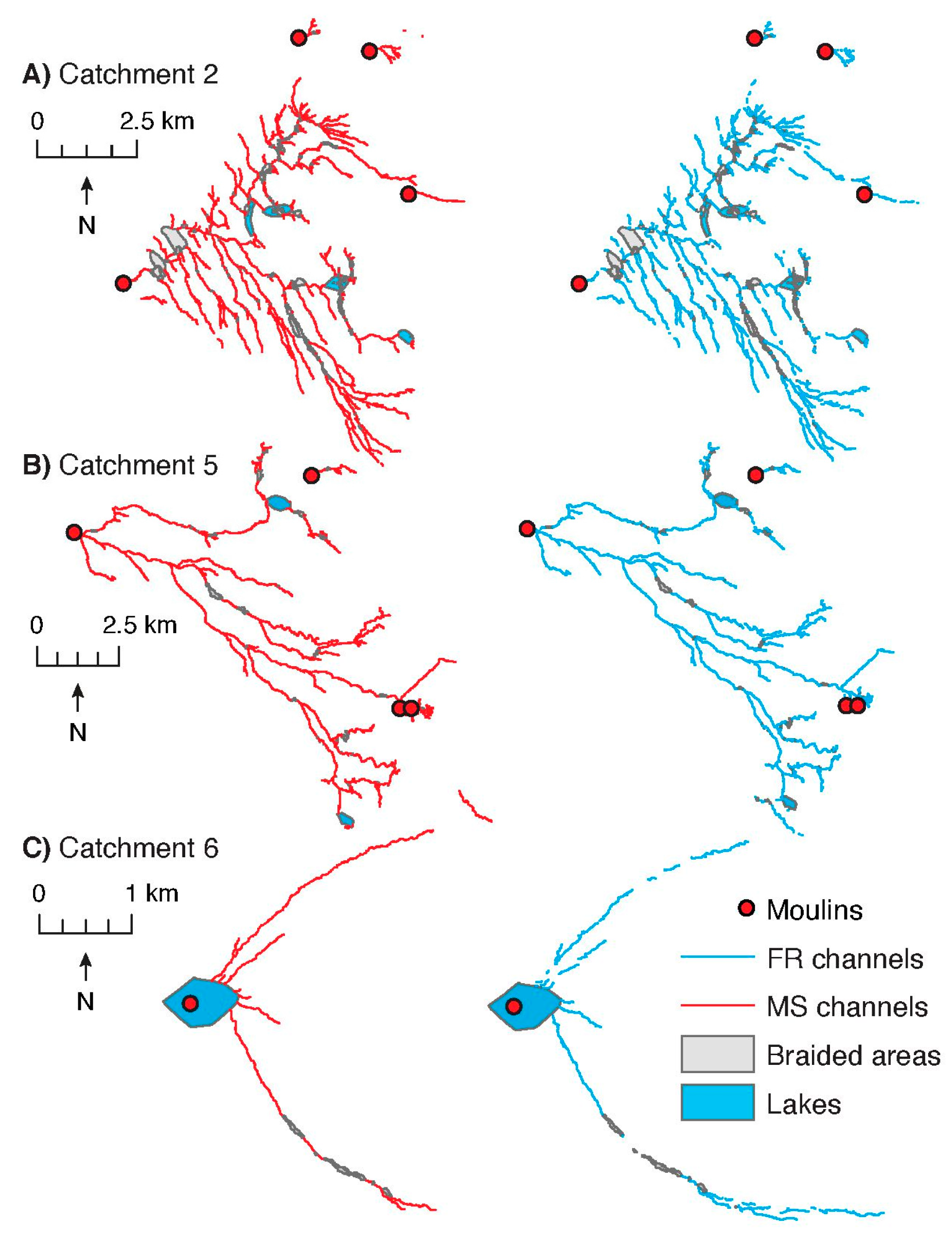
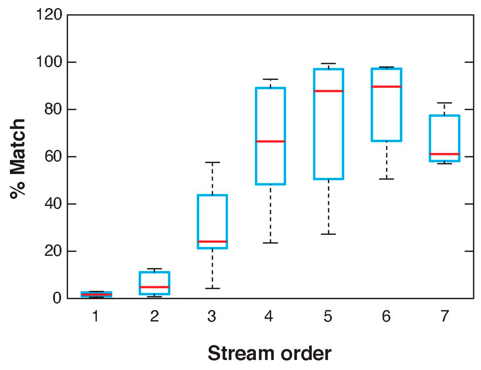
3.1.2. Comparison of Drainage Networks
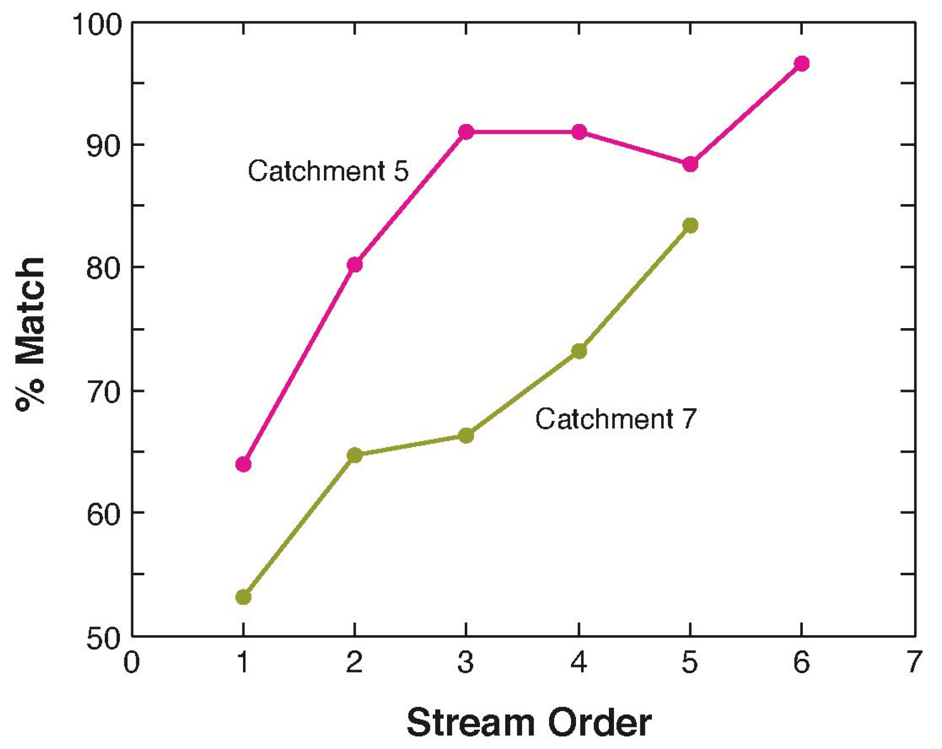
3.2. Comparison with Manually Digitized Datasets
3.2.1. High-Elevation Catchment
3.2.2. Low-Elevation Catchment
4. Discussion
4.1. Moulins
4.2. Flow Routing in High-Elevation Catchments
4.3. Flow Routing in Low-Elevation Catchments
4.4. Limitations and Considerations
5. Conclusions
Supplementary Materials
Acknowledgments
Author Contributions
Conflicts of Interest
References
- Knighton, A. Channel form and flow characteristics of supraglacial streams, Austre Okstindbreen, Norway. Arct. Alp. Res. 1981, 13, 295–306. [Google Scholar] [CrossRef]
- Smith, L.C.; Chu, V.W.; Yang, K.; Gleason, C.J.; Pitcher, L.H.; Rennermalm, A.K.; Legleiter, C.J.; Behar, A.E.; Overstreet, B.T.; Moustafa, S.E.; et al. Efficient meltwater drainage through supraglacial streams and rivers on the southwest Greenland ice sheet. Proc. Natl. Acad. Sci. USA 2015, 112, 1001–1006. [Google Scholar] [CrossRef] [PubMed]
- Wyatt, F.R.; Sharp, M.J. Linking surface hydrology to flow regimes and patterns of velocity variability on Devon Ice Cap, Nunavut. J. Glaciol. 2015, 61, 387–399. [Google Scholar] [CrossRef]
- Rippin, D.M.; Pomfret, A.; King, N. High resolution mapping of supra-glacial drainage pathways reveals link between micro-channel drainage density, surface roughness and surface reflectance. Earth Surf. Process. Landf. 2015, 40, 1279–1290. [Google Scholar] [CrossRef]
- Karlstrom, L.; Gajjar, P.; Manga, M. Meander formation in supraglacial streams. J. Geophys. Res. Earth Surf. 2013, 118, 1897–1907. [Google Scholar] [CrossRef]
- Yang, K.; Smith, L.C. Internally drained catchments dominate supraglacial hydrology of the southwest Greenland Ice Sheet. J. Geophys. Res. Earth Surf. 2016, 121, 1891–1910. [Google Scholar] [CrossRef]
- Gleason, C.J.; Smith, L.C.; Chu, V.W.; Legleiter, C.J.; Pitcher, L.H.; Overstreet, B.T.; Rennermalm, A.K.; Forster, R.R.; Yang, K. Characterizing supraglacial meltwater channel hydraulics on the Greenland Ice Sheet from in situ observations. Earth Surf. Process. Landf. 2016, 41, 2111–2122. [Google Scholar] [CrossRef]
- Yang, K.; Smith, L.C.; Chu, V.W.; Pitcher, L.H.; Gleason, C.J.; Rennermalm, A.K.; Li, M. Fluvial morphometry of supraglacial river networks on the southwest Greenland Ice Sheet. GISci. Remote Sens. 2016, 53, 459–482. [Google Scholar] [CrossRef]
- Dozier, J. Part II: Channel adjustments in supraglacial stream. In Studies of Morphology and Stream Action on Ablating Ice; Arctic Institute of North America: Montreal, QC, Canada, 1970; pp. 69–117. [Google Scholar]
- Karlstrom, L.; Yang, K. Fluvial supraglacial landscape evolution on the Greenland Ice Sheet. Geophys. Res. Lett. 2016, 43, 2683–2692. [Google Scholar] [CrossRef]
- Sundal, A.V.; Shepherd, A.; Nienow, P.; Hanna, E.; Palmer, S.; Huybrechts, P. Melt-induced speed-up of Greenland ice sheet offset by efficient subglacial drainage. Nature 2011, 469, 521–524. [Google Scholar] [CrossRef] [PubMed]
- Banwell, A.F.; Willis, I.C.; Arnold, N.S. Modeling subglacial water routing at Paakitsoq, W Greenland. J. Geophys. Res. Earth Surf. 2013, 118, 1282–1295. [Google Scholar] [CrossRef]
- Joughin, I.; Das, S.B.; Flowers, G.E.; Behn, M.D.; Alley, R.B.; King, M.A.; Smith, B.E.; Bamber, J.L.; Van Den Broeke, M.R.; Van Angelen, J.H. Influence of ice-sheet geometry and supraglacial lakes on seasonal ice-flow variability. Cryosphere 2013, 7, 1185–1192. [Google Scholar] [CrossRef]
- Schoof, C. Ice-sheet acceleration driven by melt supply variability. Nature 2010, 468, 803–806. [Google Scholar] [CrossRef] [PubMed]
- Van de Wal, R.; Boot, W.; van den Broeke, M.; Smeets, C.; Reijmer, C.; Donker, J.; Oerlemans, J. Large and rapid melt-induced velocity changes in the ablation zone of the Greenland ice sheet. Science. 2008, 321, 111–114. [Google Scholar] [CrossRef] [PubMed]
- Noh, M.-J.; Howat, I.M. Automated stereo-photogrammetric DEM generation at high latitudes: Surface Extraction with TIN-based Search-space Minimization (SETSM) validation and demonstration over glaciated regions. GISci. Remote Sens. 2015, 52, 198–217. [Google Scholar] [CrossRef]
- Yang, K.; Smith, L.C. Supraglacial streams on the greenland ice sheet delineated from combined spectral–shape information in high-resolution satellite imagery. IEEE Geosci. Remote Sens. Lett. 2013, 10, 801–805. [Google Scholar] [CrossRef]
- DGGS Staff. Elevation Datasets of Alaska: Alaska Division of Geological and Geophysical Surveys Digital Data Series 4 2013. Available online: http://maps.dggs.alaska.gov/elevationdata/ (accessed on 30 November 2016).
- High Resolution Lidar Digital Elevation Models and Low Resolution Shaded Relief Maps of Antarctica from USGS. Available online: http://nsidc.org/data/ANTARCTIC_DEM (accessed on 30 November 2016).
- Shean, D.E.; Alexandrov, O.; Moratto, Z.M.; Smith, B.E.; Joughin, I.R.; Porter, C.; Morin, P. An automated, open-source pipeline for mass production of digital elevation models (DEMs) from very-high-resolution commercial stereo satellite imagery. ISPRS J. Photogramm. Remote Sens. 2016, 116, 101–117. [Google Scholar] [CrossRef]
- Fountain, A.; Walder, J. Water flow through temperate glaciers. Rev. Geophys. 1998, 36, 299–328. [Google Scholar] [CrossRef]
- Irvine-Fynn, T.D.L.; Hodson, A.J.; Moorman, B.J.; Vatne, G.; Hubbard, A.L. Polythermal glacier hydrology: A review. Rev. Geophys. 2011, 49, 1–37. [Google Scholar] [CrossRef]
- Ferguson, R. Sinuosity of supraglacial streams. Geol. Soc. Am. Bull. 1973, 251–255. [Google Scholar] [CrossRef]
- Parker, G. Meadering of supraglacial melt streams. Water Resour. Res. 1975, 11, 551–552. [Google Scholar] [CrossRef]
- Dozier, J. An examination of the variance minimization tendencies of a supraglacial stream. J. Hydrol. 1976, 31, 359–380. [Google Scholar] [CrossRef]
- Marston, R.A. Supraglacial Stream Dynamics on the Juneau Icefield. Ann. Assoc. Am. Geogr. 2015, 73, 597–608. [Google Scholar] [CrossRef]
- Iken, A. The effect of the subglacial water pressure on the sliding velocity of a glacier in an idealized numerical model. J. Glaciol. 1981, 27, 407–421. [Google Scholar]
- Thomsen, H.H. Photogrammetric and satellite mapping of the margin of the inland ice, West Greenland. Ann. Glaciol. 1986, 8, 164–167. [Google Scholar]
- Lampkin, D.J.; VanderBerg, J. Supraglacial melt channel networks in the Jakobshavn Isbrae region during the 2007 melt season. Hydrol. Process. 2014, 28, 6038–6053. [Google Scholar] [CrossRef]
- Fitzpatrick, A.A.W.; Hubbard, A.L.; Box, J.E.; Quincey, D.J.; Van As, D.; Mikkelsen, A.P.B.; Doyle, S.H.; Dow, C.F.; Hasholt, B.; Jones, G.A. A decade (2002–2012) of supraglacial lake volume estimates across Russell Glacier, West Greenland. Cryosphere 2014, 8, 107–121. [Google Scholar] [CrossRef]
- McGrath, D.; Colgan, W.; Steffen, K.; Lauffenburger, P.; Balog, J. Assessing the summer water budget of a moulin basin in the sermeq avannarleq ablation region, Greenland ice sheet. J. Glaciol. 2011, 57, 954–964. [Google Scholar] [CrossRef]
- Das, S.; Joughin, I.; Behn, M.; Howat, I.; King, M.; Lizarralde, D.; Bhatia, M. Fracture propagation to the base of the Greenland ice sheet during supraglacial lake drainage. Science 2008, 320, 778–782. [Google Scholar] [CrossRef] [PubMed]
- Poinar, K.; Joughin, I.; Das, S.B.; Behn, M.D.; Lenaerts, J.T.M.; Van Den Broeke, M.R. Limits to future expansion of surface-melt-enhanced ice flow into the interior of western Greenland. Geophys. Res. Lett. 2015, 42, 1800–1807. [Google Scholar] [CrossRef]
- Yang, K.; Smith, L.C.; Chu, V.W.; Gleason, C.J.; Li, M. A Caution on the Use of Surface Digital Elevation Models to Simulate Supraglacial Hydrology of the Greenland Ice Sheet. IEEE J. Sel. Top. Appl. Earth Obs. Remote Sens. 2015, 8, 5212–5224. [Google Scholar] [CrossRef]
- Banwell, A.F.; Arnold, N.S.; Willis, I.C.; Tedesco, M.; Ahlstrøm, A.P. Modeling supraglacial water routing and lake filling on the Greenland Ice Sheet. J. Geophys. Res. 2012, 117, 1–11. [Google Scholar] [CrossRef]
- Arnold, N.S.; Banwell, A.F.; Willis, I.C. High-resolution modelling of the seasonal evolution of surface water storage on the Greenland Ice Sheet. Cryosphere 2014, 8, 1149–1160. [Google Scholar] [CrossRef]
- Andrews, L.C. Spatial and Temporal Evolution of the Glacial Hydrologic System of the Western Greenland Ice Sheet: Observational and Remote Sensing Results. Ph.D. Thesis, University of Texas at Austin, Austin, TX, USA, 2015. [Google Scholar]
- Tarboton, D.G.; Bras, R.L.; Rodriguiez-Iturbe, I. On the extraction of channel networks from digital elevation data. Hydrol. Process. 1991, 5, 81–100. [Google Scholar] [CrossRef]
- Arnold, N. A new approach for dealing with depressions in digital elevation models when calculating flow accumulation values. Prog. Phys. Geogr. 2010, 34, 781–809. [Google Scholar] [CrossRef]
- Gulley, J.D.; Benn, D.I.; Screaton, E.; Martin, J. Mechanisms of englacial conduit formation and their implications for subglacial recharge. Quat. Sci. Rev. 2009, 28, 1984–1999. [Google Scholar] [CrossRef]
- Nienow, P.; Hubbard, B. Surface and Englacial Drainage of Glaciers and Ice Sheets. Encycl. Hydrol. Sci. 2005. [Google Scholar] [CrossRef]
- Conrad, O.; Bechtel, B.; Bock, M.; Dietrich, H.; Fischer, E.; Gerlitz, L.; Wehberg, J.; Wichmann, V.; Bohner, J. System for Automated Geoscientific Analyses (SAGA). Geosci. Model Dev. 2015, 8, 1991–2007. [Google Scholar] [CrossRef]
- ESRI ArcGIS Desktop: Release 10.3.1 2016; Environmental Systems Research Institute: Redlands, CA, USA, 2016.
- GRASS Development Team Geographic Resources Analysis Support System (GRASS) Software 2015. Available online: https://grass.osgeo.org/ (accessed on 30 November 2016).
- Maidment, D. Arc Hydro: GIS for Water Resources; ESRI Inc.: Redlands, CA, USA, 2002. [Google Scholar]
- Jóhannesson, T.; Björnsson, H.; Pálsson, F.; Sigurðsson, O.; Þorsteinsson, Þ. LiDAR mapping of the Snæfellsjökull ice cap, western Iceland. Jökull 2003, 61, 19–32. [Google Scholar]
- Clason, C.C.; Mair, D.W.F.; Nienow, P.W.; Bartholomew, I.D.; Sole, A.; Palmer, S.; Schwanghart, W. Modelling the transfer of supraglacial meltwater to the bed of Leverett Glacier, Southwest Greenland. Cryosphere 2015, 9, 123–138. [Google Scholar] [CrossRef]
- Ewing, K. Part II: Supraglacial streams on the Kaskawulsh glacier, Yukon Territory. In Studies of Morphology and Stream Action on Ablating Ice; Arctic Institute of North America: Montreal, QC, Canada, 1970; pp. 131–167. [Google Scholar]
- Nghiem, S.V.; Hall, D.K.; Mote, T.L.; Tedesco, M.; Albert, M.R.; Keegan, K.; Shuman, C.A.; DiGirolamo, N.E.; Neumann, G. The extreme melt across the Greenland ice sheet in 2012. Geophys. Res. Lett. 2012, 39, 6–11. [Google Scholar] [CrossRef]
- O’Callaghan, J.F.; Mark, D.M. The extraction of drainage networks from digital elevation data. Comput. Vis. Graph. Image Process. 1984, 28, 323–344. [Google Scholar] [CrossRef]
- Schwanghart, W.; Kuhn, N. TopoToolbox: A set of Matlab functions for topographic analysis. Environ. Model. Softw. 2010, 25, 770–781. [Google Scholar] [CrossRef]
- Montgomery, D.; Foufoula-Georgiou, E. Channel network source representation using digital elevation models. Water Resour. Res. 1993, 29, 3925–3934. [Google Scholar] [CrossRef]
- Kamintzis, J. The Spatial Dynamics of An Annual Supraglacial Meltwater Channel in the Ablation Zone of Haut Glacier d’Arolla, Switzerland; Aberyswyth University: Aberystwyth, UK, 2015. [Google Scholar]
- Stenborg, T. Glacier drainage connected with ice structures. Geogr. Ann. Ser. A Phys. Geogr. 1968, 50, 25–53. [Google Scholar] [CrossRef]
- Brykała, D. Evolution of supraglacial drainage on Waldemar Glacier (Spitsbergen) in the period 1936–1998. In Proceedings of the Polish Polar Studies: 25th International Polar Symposium, Warsaw, Poland, 16–17 September 1998; pp. 247–261.
- Hodgkins, R. Glacier hydrology in Svalbard, Norwegian High Arctic. Quat. Sci. Rev. 1997, 16, 957–973. [Google Scholar] [CrossRef]
- Fountain, A.G. Effect of Snow and Firn Hydrology on the Physical and Chemical Characteristics of Glacial Runoff. Hydrol. Process. 1996, 10, 509–521. [Google Scholar] [CrossRef]
- Onesti, L.J. Slushflow release mechanism: A first approximation. In Avalanche Formation, Movement and Effect; IAHS: Wallingford, UK, 1987; pp. 331–336. [Google Scholar]
- Mantelli, E.; Camporeale, C.; Ridolfi, L. Supraglacial channel inception: Modeling and processes. Water Resour. Res. 2015, 51, 7044–7063. [Google Scholar] [CrossRef]
- Montgomery, D.; Dietrich, W. Landscape dissection and drainage area-slope thresholds. In Process Models and Theoretical Geomorphology; Kirkby, M., Ed.; John Wiley & Sons Ltd.: Hoboken, NJ, USA, 1994; p. 417. [Google Scholar]
- Tucker, G.; Bras, R. Hillslope processes, drainage density, and landscape morphology. Water Resour. Res. 1998, 34, 2751–2764. [Google Scholar] [CrossRef]
- Montgomery, D.R.; Dietrich, W.E. Where do channels begin? Nature 1988, 336, 232–234. [Google Scholar] [CrossRef]
- Zhang, W.; Montgomery, D. Digital elevation model grid size, landscape representation, and hydrologic simulations. Water Resour. Res. 1994, 30, 1019–1028. [Google Scholar] [CrossRef]
- Doctor, D.H.; Young, J.A. An evaluation of Automated Gis Tools for Delineating Karst Sinkholes and Closed Depressions From 1-Meter Lidar-Derived Digital Elevation Data. In Proceedings of the 13th Multidisciplinary Conference on Sinkholes and the Engineering and Environmental Impacts of Karst, Carlsbad, NM, USA, 6–10 May 2013; pp. 449–458.
- Tarboton, D. A new method for the determination of flow directions and upslope areas in grid digital elevation models. Water Resour. Res. 1997, 33, 309–319. [Google Scholar] [CrossRef]
- Van de Wal, R.S.W.; Boot, W.; Smeets, C.J.P.P.; Snellen, H.; van den Broeke, M.R.; Oerlemans, J. Twenty-one years of mass balance observations along the K-transect, West Greenland. Earth Syst. Sci. Data 2012, 4, 31–35. [Google Scholar] [CrossRef]
- Mikkelsen, A.B.; Hubbard, A.; Macferrin, M.; Eric Box, J.; Doyle, S.H.; Fitzpatrick, A.; Hasholt, B.; Bailey, H.L.; Lindbäck, K.; Pettersson, R. Extraordinary runoff from the Greenland ice sheet in 2012 amplified by hypsometry and depleted firn retention. Cryosphere 2016, 10, 1147–1159. [Google Scholar] [CrossRef]
- Palmer, S.; Shepherd, A.; Nienow, P.; Joughin, I. Seasonal speedup of the Greenland Ice Sheet linked to routing of surface water. Earth Planet. Sci. Lett. 2011, 302, 423–428. [Google Scholar] [CrossRef]
- Colgan, W.; Steffen, K. Modelling the spatial distribution of moulins near Jakobshavn, Greenland. In Proceedings of the IOP Conference Series: Earth and Environmental Science, Copenhagen, Denmark, 10–12 March 2009.
- Clason, C.; Mair, D.W.F.; Burgess, D.O.; Nienow, P.W. Modelling the delivery of supraglacial meltwater to the ice/bed interface: Application to southwest Devon Ice Cap, Nunavut, Canada. J. Glaciol. 2012, 58, 361–374. [Google Scholar] [CrossRef]
- Rodriguiez-Iturbe, I.; Rinaldo, A. Fractal River Basins: Chance and Self-Organization; Cambridge University Press: Cambridge, UK, 1997. [Google Scholar]
- Yang, K.; Karlstrom, L.; Smith, L.C.; Li, M. Automated High-Resolution Satellite Image Registration Using Supraglacial Rivers on the Greenland Ice Sheet. IEEE J. Sel. Top. Appl. Earth Obs. Remote Sens. 2016. [Google Scholar] [CrossRef]


| Channel Extraction Method | Imagery Source | Acquisition Date(s) | Resolution (m) | Reference |
|---|---|---|---|---|
| Flow Routing (FR) | SETSM DEM (derived from WorldView-1) | 24 July 2012 (Catchments 1–3) | 2.0 | [16] |
| 20 August 2012 (Catchments 4 and 5) | ||||
| 20 August 2011 (Catchment 6) | ||||
| Multispectral (MS) | WorldView-2 | 18–23 July 2012 | 2.0 | [2] |
| Manual Digitizing (MD) | WorldView-1 | 21 July 2012 (Catchment 7) | 0.5 | n/a |
| 20 August 2012 (Catchment 5) |
| Catchment | Central Coordinates | Area (km2) | Mean Slope (%) | Mean Elevation (m) | Datasets | ||
|---|---|---|---|---|---|---|---|
| FR | MS | MD | |||||
| 1 | 49°12′48.853″W | 23.1 | 11.0 | 1172 | X | X | |
| 67°15′3.539″N | |||||||
| 2 | 49°13′58.816″W | 71.5 | 11.9 | 1147 | X | X | |
| 67°8′52.932″N | |||||||
| 3 | 49°11′56.907″W | 15.5 | 10.7 | 1230 | X | X | |
| 67°13′15.191″N | |||||||
| 4 | 49°14′5.529″W | 78.2 | 11.6 | 1119 | X | X | |
| 67°2′24.692″N | |||||||
| 5 | 48°52′8.931″W | 79.2 | 13.0 | 1244 | X | X | X |
| 66°41′56.575″N | |||||||
| 6 | 48°18′22.375″W | 31.2 | 8.2 | 1528 | X | X | |
| 66°55′17.935″N | |||||||
| 7 | 49°44′22.47″W | 42.2 | 16.1 | 838 | X | X | |
| 67°6′19.874″N | |||||||
| Catchment | Missed Moulins | MS Drainage Density (km/km2) | MS Initiation Threshold (km2) | |
|---|---|---|---|---|
| Number | Area Drained | |||
| 1 | 0 | 0.0% | 2.8 | 0.3 |
| 2 | 3 | 8.0% | 2.2 | 0.5 |
| 3 | 0 | 0.0% | 2.4 | 0.3 |
| 4 | 3 | 1.4% | 2.0 | 0.5 |
| 5 | 3 | 1.9% | 1.4 | 0.8 |
| 6 | 0 | 0.0% | 0.6 | 1.8 |
© 2016 by the authors; licensee MDPI, Basel, Switzerland. This article is an open access article distributed under the terms and conditions of the Creative Commons Attribution (CC-BY) license (http://creativecommons.org/licenses/by/4.0/).
Share and Cite
King, L.; Hassan, M.A.; Yang, K.; Flowers, G. Flow Routing for Delineating Supraglacial Meltwater Channel Networks. Remote Sens. 2016, 8, 988. https://doi.org/10.3390/rs8120988
King L, Hassan MA, Yang K, Flowers G. Flow Routing for Delineating Supraglacial Meltwater Channel Networks. Remote Sensing. 2016; 8(12):988. https://doi.org/10.3390/rs8120988
Chicago/Turabian StyleKing, Leonora, Marwan A. Hassan, Kang Yang, and Gwenn Flowers. 2016. "Flow Routing for Delineating Supraglacial Meltwater Channel Networks" Remote Sensing 8, no. 12: 988. https://doi.org/10.3390/rs8120988
APA StyleKing, L., Hassan, M. A., Yang, K., & Flowers, G. (2016). Flow Routing for Delineating Supraglacial Meltwater Channel Networks. Remote Sensing, 8(12), 988. https://doi.org/10.3390/rs8120988