Joint Time-Frequency Signal Processing Scheme in Forward Scattering Radar with a Rotational Transmitter

Abstract

This paper explores the concept of a Forward Scattering Radar (FSR) system with a rotational transmitter for target detection and localization. Most of the research and development in FSR used a fixed dedicated transmitter; therefore, the detection of stationary and slow moving target is very difficult. By rotating the transmitter, the received signals at the receiver contain extra information carried by the Doppler due to the relative movement of the transmitter-target-receiver. Hence, rotating the transmitter enhances the detection capability especially for a stationary and slow-moving target. In addition, it increases the flexibility of the transmitter to control the signal direction, which broadens the coverage of FSR networks. In this paper, a novel signal processing for the new mode of FSR system based on the signal’s joint time-frequency is proposed and discussed. Additionally, the concept of the FSR system with the rotational transmitter is analyzed experimentally for the detection and localization of a stationary target, at very low speed and a low profile target crossing the FSR baseline. The system acts as a virtual fencing of a remote sensor for area monitoring. The experimental results show that the proposed mode with the new signal processing scheme can detect a human intruder. The potential applications for this system could be used for security and border surveillance, debris detection on an airport runway, ground aerial monitoring, intruder detection, etc.

1. Introduction

Forward Scattering Radar (FSR) is a specific condition in bistatic radar mode and is gaining special attention from the modern radar community lately. In theory, for target detection in an FSR system to be effective, it utilizes the electromagnetic wave scattered by the target to the receiver [1]. The technical requirement in FSR, which needs the target to be in proximity to the baseline of the transmitter-receiver, restricts the operation to within narrow angles. Furthermore, the Doppler ‘dead zone’ (very low Doppler frequencies) and loss of range resolution limits the practicality of FSR. However, FSR has a number of unique qualities that make it useful for remote monitoring. One of the special characteristics is the high amplitude target’s Radar Cross-Section (RCS) at the forward scatter position. The enhancement in forward scatter RCS, which exists within the Forward Scatter Main Lobe (FSML), can be perceived within the optical region and the specific scenario in the Mie region [2,3]. Moreover, the target’s RCS in FSR does not affected by the Radar Absorbing Material (RAM) coating, as well as the diamond shape of some targets to reduce RCS. As a result, the FSR system is not affected by “stealth” technology.

One of the earliest publications of the FSR system was dedicated to air target detection and tracking [4,5,6]. The FSR used the fixed transmitter–receiver pair, and the target flew crossing the baseline between the FSR systems. Later, FSR was tested for ground target detection and classification, but still used a fixed transmitter-receiver pair [7,8,9]. Signal processing and signal modeling of FSR are explained in [10]. The FSR system has also been tested for maritime applications [10,11,12]. Recently, new research in FSR is to integrate with MIMO architecture [13] and operate as a passive radar [14,15].

Although the number of research works in FSR has increased, the main published manuscripts and reported work on FSR focus on the fixed transmitter and utilize the relative movement of the target for detection and tracking. In this condition, the detection is restricted to the narrow coverage of FSML, and it is highly dependent on the target speed. A low target speed will give a low Doppler frequency and make the detection difficult. Moreover, the detection is almost impossible for a stationary target. However, if the transmitter can be controlled, for example, it can be mechanically rotated with a certain rotational speed, it offers some degree of freedom. By rotating the transmitter, the received signals at the receiver contain extra information carried by the Doppler due to relative movement of the transmitter-target-receiver. Hence, rotating the transmitter enhances the detection sensitivity especially for stationary and slow moving targets. By manipulating the Doppler frequency at the receiver, the FSR system becomes more flexible and practical. Additionally, it can also increase the coverage with multiple receivers that could be arranged in such a way; the receivers reside within the transmitter antenna beam width. Though the angular movement of the transmitter creates extra Doppler effects at the receiver, consequently the signal processing is different from the conventional FSR signal processing.

The aim of this paper is to explore the concept of the FSR system with a rotational transmitter. The specific objective is to develop the detection and localization technique of stationary, as well as a very slow-moving target within the FSR region. The idea is proven by deploying the system for a remote security monitoring, which must be capable of detecting and locating an intruder. The intruder is either almost stationary or slow moving with low profile attributes. The detail derivation of the theoretical signal model at the output of ADC is explained in this paper, although a simplified version was presented in [16]. A novel detection technique based on the signal’s joint Time-Frequency (T-F) is integrated with the proposed FSR system. Two methods of signal pre-processing were tested and implemented on the signal acquired from the experimentation. Both methods exploit the difference in the Doppler effect at the receiver due to the relative angular movement of the transmitter with and without the target. The adaptation of the rotational transmitter concept to the conventional FSR system provides a new emerging area of research. Thus, the new concept of the FSR system can be functional in diverse potential applications, such as: remote security and border surveillance, close range security applications intended for humans, animal and man-made object detection, foreign object debris (FOD) detection on an airport runway where most of the objects are stationary, etc. Nevertheless, with the appropriate modification, the technique is applicable to air and maritime targets.

The paper is organized as follows: Section 2 presents the common FSR layout. Then, the same section explains the new FSR system with the angular movement of the transmitter. The detail derivation of the signal model and comparison to the controlled experimental result are also given in this section. Section 3 elaborates the experimental setup of the proposed system, as well as the experimentation with the practical application of intruder detection. Section 4 is divided into two parts, with each part discussing slightly different signal pre-processing schemes that can be integrated with the system. The first part explains the detection and localization for a stationary target followed by a slow moving target in the later part. The paper is concluded in Section 5.

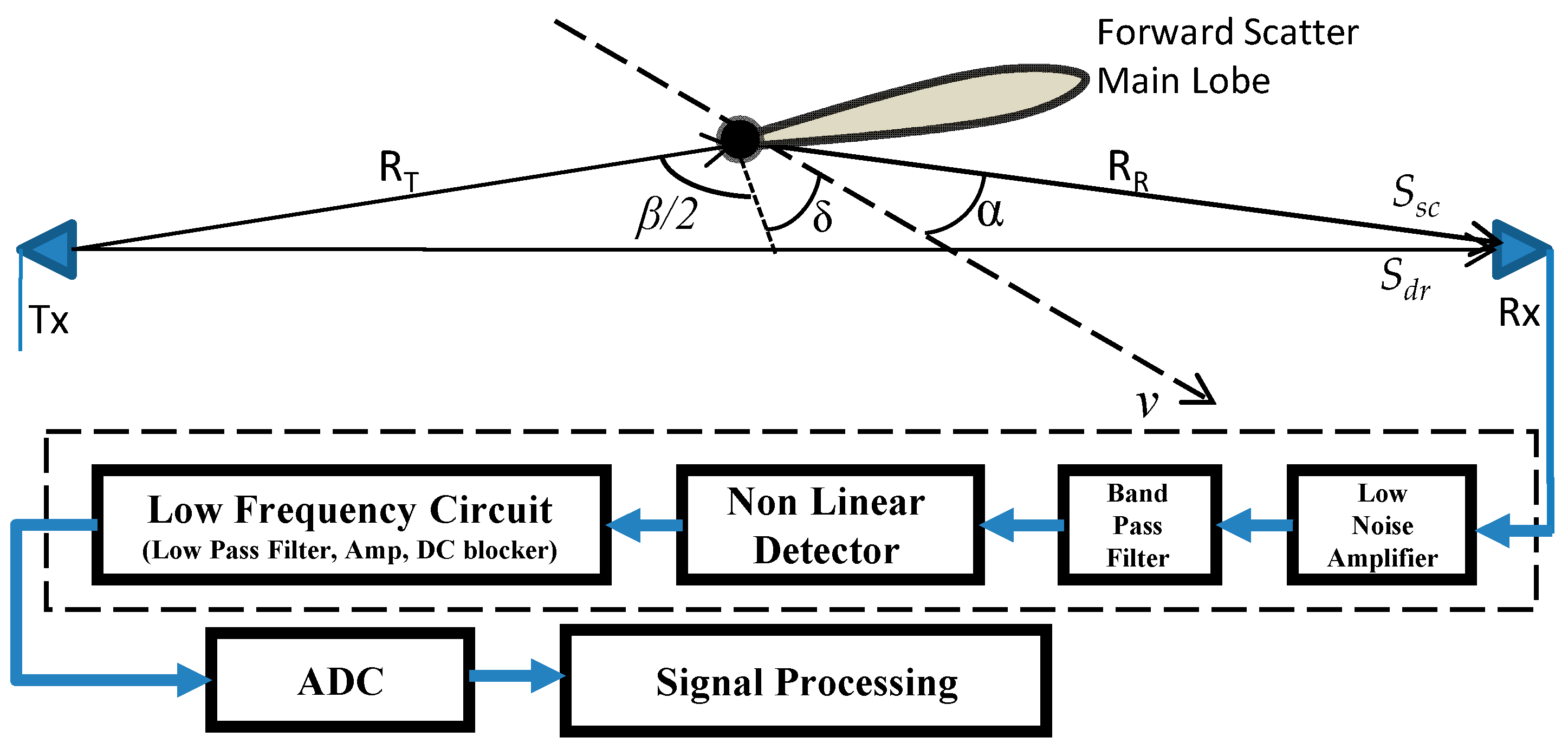
2. FSR System Topology and Overview

The simplified geometrical layout of the FSR system is illustrated in Figure 1. The transmitter can transmit any type of modulated signal due to the non-dependent forward scatter signal processing to the types of signal transmitted at the receiver system [15,16]. In a conventional FSR system, the received signal consists of a direct signal from the transmitter and forward scattered signal from the target. A moving target will introduce the Doppler shift in the scattered signal [1,7]. The Doppler signal is then extracted and analyzed for target detection and identification. As long as the direct signal is greater than the receiver thermal noise, any type of non-linear component (for example, s diode detector) can be used as the mixer. In the forward scatter case, the direct signal is used as a heterodyne to the scattered signal form the target.

Based on Figure 1, the direct signal from the transmitter, S_dr, with carrier frequency f_o (assume phase noise free) and a signal scattered from a target, S_sc, with a Doppler shift, f_sc is given by (1) and (2), respectively [16,17]. There exists a phase change in the Doppler signal scattered by the transmitter as explained by Babinet’s principle [18,19]. In the simplified manner, the signal at the input of the receiver S_rx is a combination between S_dr and S_sc, which can be expressed in Equation (3):

S_dr(t) = A_dr cos((ω_o)t)

(1)

S_sc(t) = A_sc sin((ω_o + ω_sc)t)

(2)

S_rx(t) = S_dr(t) + S_sc(t) = A_dr cos((ω_o)t) + A_sc sin((ω_o + ω_sc)t)

(3)

where ω_o = 2πf_o and ω_sc = 2πf_sc. A_dr and A_sc denote the amplitudes of the direct path signal (leakage) and the target scattered signal, respectively. The FSR circuits used a non-linear element as the detection mechanism with the transfer characteristics of Y_out = (Y_in)²; hence, at the output of the non-linear element, the signal is given by:

$${\mathrm{Y}}_{\mathrm{out}}\left(\mathrm{t}\right)={\left({\mathrm{A}}_{\mathrm{dr}}\cos \left({\mathsf{\omega }}_{\mathrm{o}}\mathrm{t}\right)+{\mathrm{A}}_{\mathrm{sc}}\sin \left(\left({\mathsf{\omega }}_{\mathrm{o}}+{\mathsf{\omega }}_{\mathrm{sc}}\right)\mathrm{t}\right)\right)}^2$$

(4)

By applying low pass filtering to the output signal from the non-linear element, the high frequency part of the signal is filtered out, leaving only two spectral components: the DC value and the Doppler from the target:

$${\mathrm{Y}}_{\mathrm{out}\_\mathrm{f}}(\mathrm{t})=\mathsf{{\rm K}}\left(({\left({\mathrm{A}}_{\mathrm{dr}}\right)}^2+{\left({\mathrm{A}}_{\mathrm{sc}}\right)}^2)+\left({\mathrm{A}}_{\mathrm{dr}}{\mathrm{A}}_{\mathrm{sc}}\sin \left({\mathsf{\omega }}_{\mathrm{sc}}\mathrm{t}\right)\right)\right)$$

(5)

where K is the conversion coefficient, which depends on the type of non-linear device.

The direct signal can be filtered out by High Pass Filter and left only Y_out = A_drA_sc.sin(ω_sct). The total Doppler frequency can be extracted by the derivation of the phase component of Equation (5).

If the target’s Doppler frequency component due to the motion relative to the transmitter and receiver is given in Equations (7) and (8), respectively, then the total target’s Doppler frequency, f_d, can be calculated as follows, the detail derivation is given in Appendix A:

$${\mathrm{f}}_{\mathrm{tx}}=(\mathrm{v}/\mathsf{\lambda })\cos (\mathsf{\beta }/2+\mathsf{\delta })$$

(6)

$${\mathrm{f}}_{\mathrm{rx}}=(\mathrm{v}/\mathsf{\lambda })\cos (\mathsf{\beta }/2-\mathsf{\delta })$$

(7)

$${\mathrm{f}}_{\mathrm{d}}=(\mathrm{v}/\mathsf{\lambda })\cos (\mathsf{\beta }/2+\mathsf{\delta })+(\mathrm{v}/\mathsf{\lambda })\cos (\mathsf{\beta }/2-\mathsf{\delta })=(2\mathrm{v}/\mathsf{\lambda })\cos \left(\mathsf{\beta }/2\right)\cos \left(\mathsf{\delta }\right)$$

(8)

Based on Equation (8), the total target’s Doppler shift is zero, corresponding to the target on the baseline ($\mathsf{\beta }$ = 180°) regardless of any values of δ and target trajectories. For $\mathsf{\beta }$ ≠ 180°, the target’s Doppler frequency is specified by the transmitter-target-receiver relative speed. The Doppler shift depends mainly on the target velocity vector components and the carrier frequency. The Doppler shift will be zero for a stationary target. In most of the publications on FSR, this Doppler shift can be used for target detection, moving target selection, speed determination and trajectory reconstruction [5,6,7,8,9,10,11,12,13,14,15]. The higher the target effective target speed, the higher the Doppler shift in the received signal. Therefore, if the target is stationary, it makes the system less sensitive for detection in the conventional FSR. It can be noted that, with the identified scenario, the FSR receiver requires a very sensitive Doppler detection, and the Doppler signal is near zero for some condition.

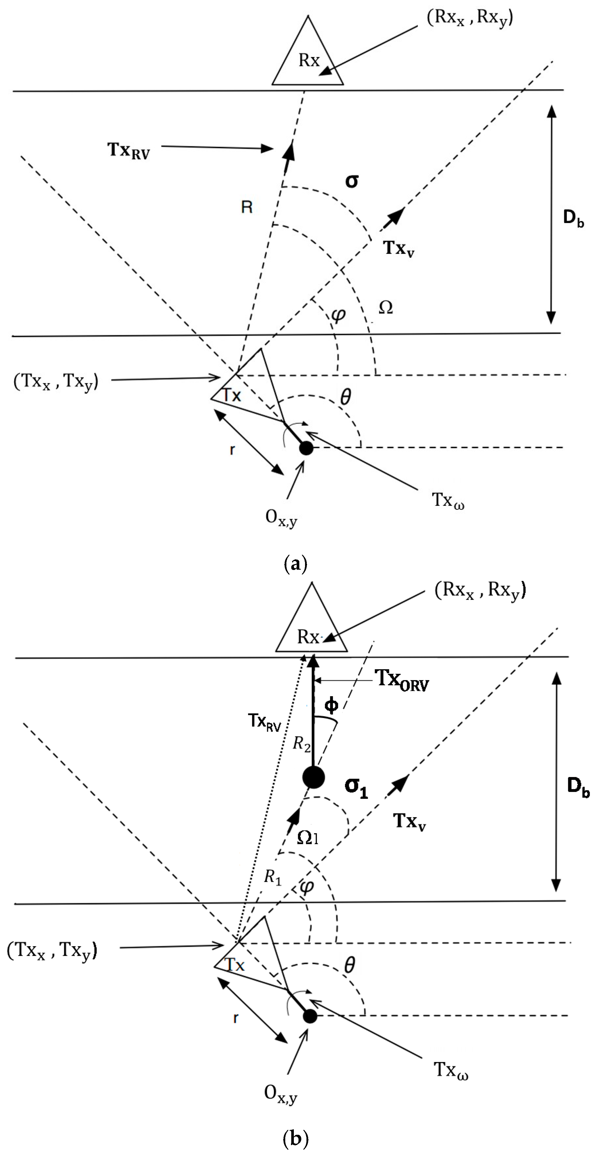
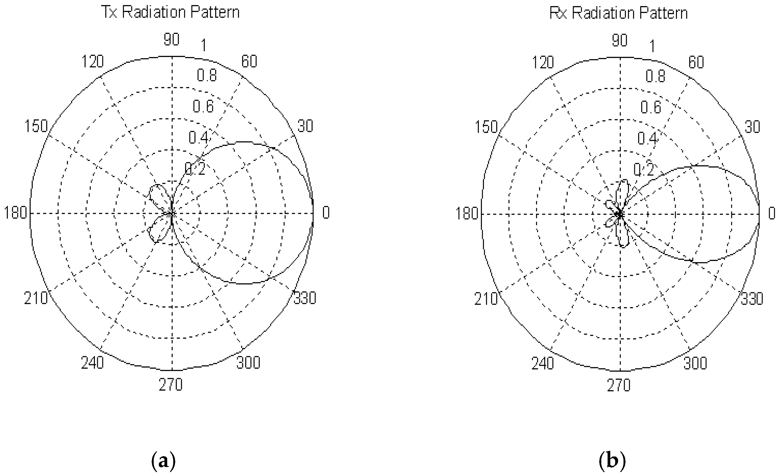
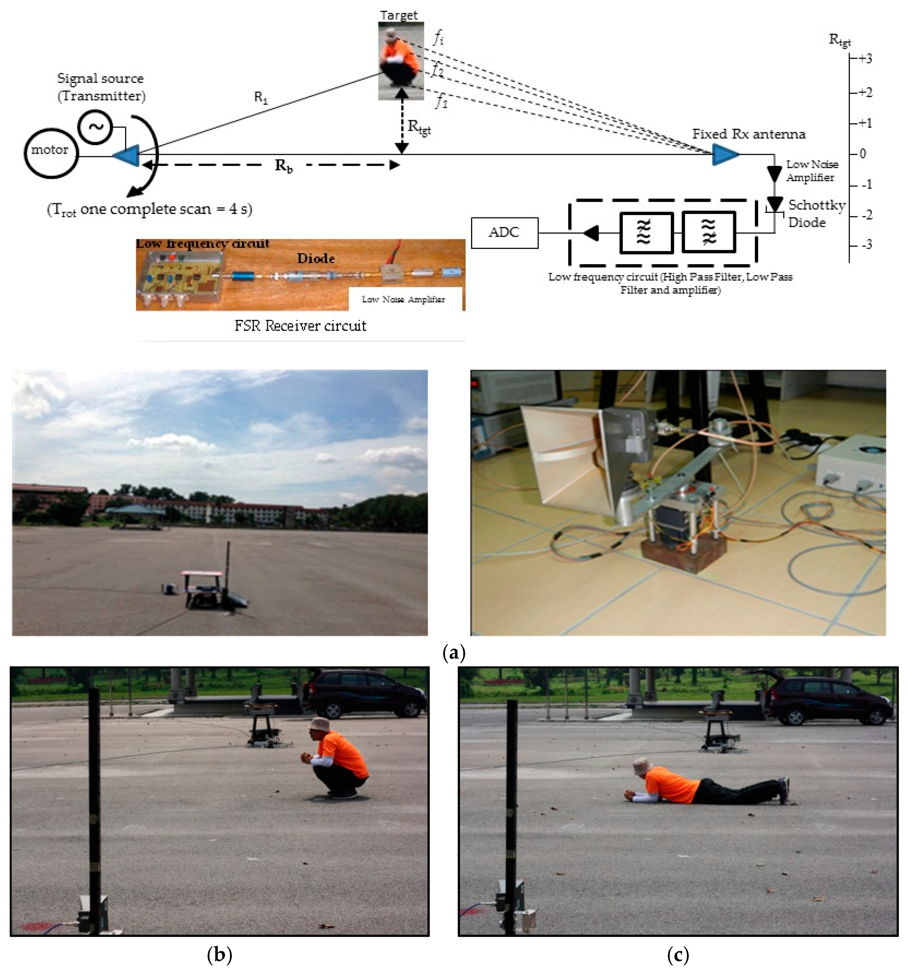
2.1. Practical Realization of FSR with Rotational Scanning Transmitter

By rotating the transmitter antenna, two Doppler shifts will exist at the receiver. First, the changing of relative velocity between the transmitter and receiver produces a direct Doppler shift in the direct received signal. The direct signal from the transmitter is always received by the receiver (regardless of the existence of an object). Second, if any object exists within the FSR region, then the relative velocity between the transmitter-target-receiver is changing, producing a scattered Doppler shift in the scattered received signal in addition to the direct signal. The proposed rotational transmitter in the FSR system with the scanning scenario setup is illustrated in Figure 2. A stationary object resides within the scanning area set by an angularly-moving transmitter and a fixed receiver. This paper concerns a stationary object, which will not be detected from the conventional FSR system because no Doppler shift exists at the receiver. The scanning can be as wide as 180° depending on the applications. A motor controlled by the computer is used for the antenna scanning movement and synchronization. The receiver will be triggered upon receiving a sufficient direct signal from the transmitter, and it is assumed within the transmitter antenna main lobe. Equations (1)–(8), which were dedicated to a fixed Tx-Rx pair and moving target crossing the baseline, need to be modified based on the new FSR layout. If an object exists, the two signals present at the input of the receiver are now:

• direct signal, S_{dr_r}, and its Doppler shift, ω_{dr_r}
• signal scattered from an object, S_{sc_r}, with scattered Doppler shift, ω_{sc_r}; hence, the signal at the input of the receiver, S_{rx_r}, will be:

  $${\mathrm{S}}_{\mathrm{dr}\_\mathrm{r}}\left(\mathrm{t}\right)={\mathrm{A}}_{\mathrm{dr}\_\mathrm{r}}\sin \left(({\mathsf{\omega }}_{\mathrm{o}}+{\mathsf{\omega }}_{\mathrm{dr}\_\mathrm{r}})\mathrm{t}\right)$$

  (9)

  $${\mathrm{S}}_{\mathrm{sc}\_\mathrm{r}}\left(\mathrm{t}\right)={\mathrm{A}}_{\mathrm{sc}\_\mathrm{r}}\sin \left(\left({\mathsf{\omega }}_{\mathrm{o}}+{\mathsf{\omega }}_{\mathrm{sc}\_\mathrm{r}}\right)\mathrm{t}\right)$$

  (10)

  $$S_{rx\_r}\left(t\right)={\mathrm{S}}_{\mathrm{dr}\_\mathrm{r}}\left(\mathrm{t}\right)+{\mathrm{S}}_{\mathrm{sc}\_\mathrm{r}}\left(\mathrm{t}\right)={\mathrm{A}}_{\mathrm{dr}\_\mathrm{r}}\sin \left(\left({\mathsf{\omega }}_{\mathrm{o}}+{\mathsf{\omega }}_{\mathrm{dr}\_\mathrm{r}}\right)\mathrm{t}\right)+{\mathrm{A}}_{\mathrm{sc}\_\mathrm{r}}\sin \left(\left({\mathsf{\omega }}_{\mathrm{o}}+{\mathsf{\omega }}_{\mathrm{sc}\_\mathrm{r}}\right)\mathrm{t}\right)$$

  (11)

where A_{dr_r} and A_{sc_r} denote the amplitudes of the direct path signal (leakage) and object scattered signal, respectively. ω_{sc_r} comprises two Doppler frequency components scattered due to the transmitter-object-receiver relative velocity. After, the non-linear element the output signal is given by:

$${\mathrm{Y}}_{\mathrm{out}\_\mathrm{r}}\left(\mathrm{t}\right)={\left({\mathrm{A}}_{\mathrm{dr}\_\mathrm{r}}\sin \left(\left({\mathsf{\omega }}_{\mathrm{o}}+{\mathsf{\omega }}_{\mathrm{dr}\_\mathrm{r}}\right)\mathrm{t}\right)+{\mathrm{A}}_{\mathrm{sc}\_\mathrm{r}}\sin \left(\left({\mathsf{\omega }}_{\mathrm{o}}+{\mathsf{\omega }}_{\mathrm{sc}\_\mathrm{r}}\right)\mathrm{t}\right)\right)}^2$$

(12)

By applying low pass filtering on the output signal, the high frequency part of the signal will be cut off, with only three spectral components remaining: DC from the direct path (leakage) signal, Doppler due to the movement of the transmitter and Doppler from the target:

$${\mathrm{Y}}_{\mathrm{out}\_\mathrm{r}\_\mathrm{f}}\left(\mathrm{t}\right)=\mathsf{\chi }\left(\left({\left({\mathrm{A}}_{\mathrm{dr}\_\mathrm{r}}\right)}^2+{\left({\mathrm{A}}_{\mathrm{sc}\_\mathrm{r}}\right)}^2\right)+\left({\mathrm{A}}_{\mathrm{dr}\_\mathrm{r}}{\mathrm{A}}_{\mathrm{sc}\_\mathrm{r}}\sin \left(\left({\mathsf{\omega }}_{\mathrm{dr}\_\mathrm{r}}+{\mathsf{\omega }}_{\mathrm{sc}\_\mathrm{r}}\right)\mathrm{t}\right)\right)\right)$$

(13)

Direct Doppler frequency f_{dr_r} and scattered Doppler frequency f_{sc_r} can be calculated by adopting the concept as illustrated in Figure 2. The direct signal path is shown by the bold line connecting the transmitter and receiver. The transmitter antenna moves with angular velocity Tx_ω attached to an arm with length r, producing tangential velocity Tx_v. The movement center of the transmitter antenna is at origin O_x,y. The relative velocity between the transmitter and receiver is changing due to the scanning mechanism; thus, direct Doppler shift is given by [14]:

$${\mathrm{f}}_{\mathrm{dr}\_\mathrm{r}}=\frac{{\mathrm{Tx}}_{\mathrm{RV}}}{\mathsf{\lambda }}=\frac{{\mathrm{Tx}}_{\mathrm{v}}\cos \mathsf{\sigma }}{\mathsf{\lambda }}$$

(14)

where Tx_v is the tangential velocity of the transmitter antenna and λ is the wavelength. The f_{dr_r} can be expressed as a function of time.

$${\mathrm{f}}_{\mathrm{d}\_\mathrm{r}}\left(\mathrm{t}\right)=\frac{1}{\mathsf{\lambda }}\left|{\mathrm{rTx}}_{\mathsf{\omega }}\cos \left(\left[{\cos }^{-1}\left(\frac{{\mathrm{Rx}}_{\mathrm{x}}-{\mathrm{Tx}}_{\mathrm{x}}}{\sqrt{{\left({\mathrm{Tx}}_{\mathrm{x}}-{\mathrm{Rx}}_{\mathrm{x}}\right)}^2+{\left({\mathrm{Tx}}_{\mathrm{y}}-{\mathrm{Rx}}_{\mathrm{y}}\right)}^2}}\right)\right]-\mathsf{\phi }\right)\right|$$

(15)

where r denotes the length of the transmitter antenna arm, φ is the direction angle of the transmitter tangential velocity, Tx_ω is the transmitter angular velocity, (Tx_x, Tx_y) and (Rx_x, Rx_y) are the transmitter and receiver position in the XY-coordinate, respectively. Tx_x, Tx_y and φ are given by the following equations:

$${\mathrm{Tx}}_{\mathrm{x}}={\mathrm{O}}_{\mathrm{x}}+\mathrm{r}\cos \left(\mathsf{\theta }\right)={\mathrm{O}}_{\mathrm{x}}+\mathrm{r}\cos \left(\left({\mathsf{\theta }}_{\mathrm{o}}+{\mathrm{Tx}}_{\mathsf{\omega }}\mathrm{t}\right)-\raisebox{1ex}{$\mathsf{\pi }$}\!\left/ \!\raisebox{-1ex}{$2$}\right.\right)$$

(16)

$${\mathrm{Tx}}_{\mathrm{y}}={\mathrm{O}}_{\mathrm{y}}+\mathrm{r}\sin \left(\mathsf{\theta }\right)={\mathrm{O}}_{\mathrm{y}}+\mathrm{r}\sin \left(\left({\mathsf{\theta }}_{\mathrm{o}}+{\mathrm{Tx}}_{\mathsf{\omega }}\mathrm{t}\right)-\raisebox{1ex}{$\mathsf{\pi }$}\!\left/ \!\raisebox{-1ex}{$2$}\right.\right)$$

(17)

$${\mathsf{\theta }}_1={\mathsf{\theta }}_{\mathrm{o}}+{\mathrm{Tx}}_{\mathsf{\omega }}\mathrm{t}$$

(18)

$$\mathsf{\phi }=\left(\mathsf{\pi }/2\right)-{\mathsf{\theta }}_1$$

(19)

$$\mathsf{\sigma }=\mathsf{\Omega }-\mathsf{\phi }$$

(20)

$$\mathsf{\Omega }={\cos }^{-1}\left(\frac{{\mathrm{Rx}}_{\mathrm{x}}-{\mathrm{Tx}}_{\mathrm{x}}}{\mathrm{R}}\right)$$

(21)

$$\mathrm{R}=\sqrt{{\left({\mathrm{Rx}}_{\mathrm{x}}-{\mathrm{Tx}}_{\mathrm{x}}\right)}^2+{\left({\mathrm{Rx}}_{\mathrm{y}}-{\mathrm{Tx}}_{\mathrm{y}}\right)}^2}$$

(22)

where: θ₁ is the angular position of the transmitter antenna (antenna look angle); θ_o indicates position of start angle; φ is the angle between the transmitter tangential velocity and reference X-axis origin coordinate; σ is the angle between the direct signal path and transmitter tangential velocity Tx_v; Ω and Ω₁ are the angles between the direct signal path and the reference X-axis transmitter antenna coordinate for the cases of the direct Doppler and the target’s scattered Doppler, respectively.

The scattered signal path from a stationary point object is shown by the bold line connecting the transmitter, object and receiver, as shown in Figure 2b, which contribute the scattered Doppler shift, ω_{sc_r}. Instantaneously-scattered Doppler frequency f_{sc_r} is given by:

$${\mathrm{f}}_{{\mathrm{sc}}_{\mathrm{r}}}=\frac{1}{\mathsf{\lambda }}\frac{\mathrm{d}\left({\mathrm{R}}_1+{\mathrm{R}}_2\right)}{\mathrm{dt}}=\frac{1}{\mathsf{\lambda }}\left[\frac{\mathrm{d}\left({\mathrm{R}}_1\right)}{\mathrm{dt}}+\frac{\mathrm{d}\left({\mathrm{R}}_2\right)}{\mathrm{dt}}\right]=\frac{1}{\lambda }\left[T{x}_v\cos \left({\sigma }_1\right)+T{x}_v\cos \left({\sigma }_1\right)\cos \left(\mathsf{\varphi }\right)\right]=Tx\_v/\lambda \left[\cos \left(\sigma \_1\right)+\cos 〖\left(\sigma \_1\right)\cos \left(\mathsf{\varphi }\right)〗\right]$$

(23)

where σ₁ is the angle formed between transmitter tangential velocity Tx_v and transmitter-object direction TxObj_vr and φ is the angle from TxObj_vr to the receiver. Equation (23) shows that the system can literally increase the Doppler frequency by adjusting the radial velocity of the transmitter. Therefore, it has some flexibility even for a very low speed (almost stationary) target. The f_{sc_r} can be represented as a factor of time by:

$${\mathrm{f}}_{\mathrm{sc}\_\mathrm{r}}(\mathrm{t})=\frac{{\mathrm{rTx}}_{\mathsf{\omega }}}{\mathsf{\lambda }}\left[\cos \left({\cos }^{-1}\left(\frac{{\mathrm{obj}}_{\mathrm{x}}-{\mathrm{Tx}}_{\mathrm{x}}}{\mathrm{R}2}\right)-\mathsf{\phi }\right)+\left(\cos \left({\cos }^{-1}\left(\frac{{\mathrm{obj}}_{\mathrm{x}}-{\mathrm{Tx}}_{\mathrm{x}}}{\mathrm{R}2}\right)-\mathsf{\phi }\right)\cos \left(\mathsf{\varphi }\right)\right)\right]$$

(24)

where Obj_x and Obj_y are the target position in the X and Y axis, respectively. σ₁, Ω₁ and R₁ are defined as below: R²

$${\mathsf{\sigma }}_1={\mathsf{\Omega }}_1-\mathsf{\phi }$$

(25)

$${\mathsf{\Omega }}_1={\cos }^{-1}\left(\frac{{\mathrm{Obj}}_{\mathrm{x}}-{\mathrm{Tx}}_{\mathrm{x}}}{\mathrm{R}2}\right)$$

(26)

$${\mathrm{R}}_1=\sqrt{{\left({\mathrm{Tx}}_{\mathrm{x}}-{\mathrm{Obj}}_{\mathrm{x}}\right)}^2+{\left({\mathrm{Tx}}_{\mathrm{y}}-{\mathrm{Obj}}_{\mathrm{y}}\right)}^2}$$

(27)

$$\mathsf{\varphi }=\left({\sin }^{-1}\left(\frac{{\mathrm{Obj}}_{\mathrm{x}}-{\mathrm{Tx}}_{\mathrm{x}}}{\mathrm{R}2}\right)\right)-{\mathsf{\Omega }}_1$$

The amplitude of the direct received signal Adr_r follows the general form of bistatic radar, which is given by Equation (22) below.

$${\mathrm{A}}_{\mathrm{dr}\_\mathrm{r}}=\frac{{\mathrm{P}}_{\mathrm{t}}{\mathrm{G}}_{\mathrm{t}}{\mathrm{G}}_{\mathrm{r}}{\mathsf{\lambda }}^2}{{\left(4\mathsf{\pi }\mathrm{R}\right)}^2}$$

(28)

where P_t is the transmitter power and G_t and G_r are the gain of the transmitting and receiving antenna, respectively. The amplitude of scattered received signal A_{sc_r} is given by:

$${\mathrm{A}}_{\mathrm{sc}\_\mathrm{r}}=\frac{{\mathrm{P}}_{\mathrm{t}}{\mathrm{G}}_{\mathrm{t}}{\mathrm{G}}_{\mathrm{r}}{\mathsf{\sigma }\mathsf{\lambda }}^2}{{\left(4\mathsf{\pi }\right)}^3{\left({\mathrm{R}}_1{\mathrm{R}}_2\right)}^2}$$

(29)

where σ denotes the forward scatter RCS of the target. Simulation on rotational forward scattering radar for static target detection has been done using MATLAB. All parameters are set to be as close to the experimental as possible, which transmit the continuous wave signal with carrier frequency f_c = 2.4 GHz at P_t = 10 dBm W. The transmitting and receiving antenna radiation patterns are illustrated in Figure 3.

An experiment to proof the signal model in Equation (14) has been implemented inside the semi-anechoic chamber with the parameters listed in

Table 1. Experiment parameters.

Parameter	Value
Antenna angular velocity (${\mathrm{Tr}}_{\mathsf{\omega }}$)	0.378π rad/s
Antenna arm length (r)	0.25 m
Rx antenna position (${\mathrm{Rx}}_{\mathrm{x},\mathrm{y}}$)	(10 m,15 m)

. Figure 4 shows the simulated and experimental received signal (no target). Both signals show some degree of similarity. However, the simulated signal can be further improved by taking into account other propagation models, such as two-ray path propagation due to the lower height of the antenna. The full ground clutter is also not integrated into the equation. Nevertheless, these signals can be used as reference signals for target detection in the new FSR system with the rotational transmitter.

Figure 5 illustrates the simulated (point target on the baseline) and experimental received signal after Doppler processing for a small metal object with size L = W = H = 2 cm at position Obj_x,y = (10, 10) m. For the simulated signal (Figure 4a and Figure 5a), the envelope shows some similarity, but it possesses an amplitude difference especially when the transmitter is parallel to the baseline. The experimental signal indicates some distortion in the received signal as compared to Figure 4b. Hence, the target detection is possible in the proposed FSR system and will be explained in the next section for the detection signal processing algorithm.

3. Practical Application of FSR with the Rotational Transmitter: Intruder Detection

The performance of the proposed FSR system with the rotational transmitter is tested on the detection of stationary and slow-moving targets. It resembles a human intruding a specific area. In this case, the radar system acts as an electronic fence in security surveillance and protecting a critical area. Intrusion detection is very important in today’s scenario. Typical detection uses an infrared fencing, camera and manual observation. Infrared cannot provide high accuracy in location and is poor during bad weather conditions, while the camera has limited accuracy during the night [20]. Manual observation by the human eye is not efficient for 24 h and remote monitoring. In contrast, the radar system can provide accurate location, working in 24 h and during bad weather conditions. By using FSR, some advantages can be obtained, especially the recognition capability and target radar cross-section enhancement. However, the detection area in the conventional FSR system is limited to the narrow coverage of the forward scatter main lobe and baseline. Hence, the proposed FSR system with the rotational transmitter can overcome this drawback, and in a practical application, it can work in hybrid mode with the existing system to increase the effectiveness for area remote monitoring.

This section presents the possible application of the proposed FSR system by practical experimentation. Three main aspects that the paper takes into consideration in the experiment and requirement are: (i) a very slow-moving intruder with start and go movement; (ii) detection of a very low profile (low altitude) ground target; and (iii) wide coverage of detection with transmitter rotation.

The experiment was conducted on a flat terrain covered with asphalt within an area of 200 m × 100 m. The FSR system transmits 2.4 GHz CW to have a higher Doppler frequency, thus increasing the detection rate. The transmitting antenna is attached to a rotational motorized control, which can be controlled by computer via an ADC. In this experiment, the transmitter was rotated 180° in the clockwise direction within, T_rot = 4 s duration for one complete rotation. The FSR system uses the receiver setup as explained in Section 2 and illustrated in Figure 6. The direct and scattered signals were recorded at the receiver side and stored in the computer. Figure 6 also shows the experimental setup and scenario for intruder detection. Rtgt in Figure 6 shows the target distance from the baseline in X-axis with origin on the transmitter receiver baseline.

Three scenarios were conducted, which are:

• Target sitting and stationary (without any movement),
• Target sitting with slightly shaking mode and
• Target moving (crawling), slowly crossing the FSR baseline.

These scenarios were chosen to replicate some typical security surveillance scenarios, like intruder behavior and debris on an airport runway. Conventional Doppler radar detects an object via Doppler shift produced by the rate of change of the total path length travelled signal between the transmitter and receiver. In the case of a static or slow-moving target, the rate of path length changes is almost zero, thus making it very difficult for the radar to detect a target. Moreover, since FSR uses CW signal, if the target is located near the baseline (FSR dead zone), it is almost impossible to extract range information from the received signal. For this reason, the transmitter is rotated to induce an object Doppler shift signal. The second reason is to have a wide area of detection coverage. Within the integration time, the received signal will acquire a direct Doppler from the transmitter, the main Doppler from the body and possibly the micro Doppler from other parts of the body, like elbow, head, leg, etc. Due to this, a wide dynamic range of Doppler frequency analysis is required in order to ensure that accurate intruder detection could be achieved.

Figure 7 shows the signal recorded, using a 50-kSps ADC, for ground clutter (no target) after scanning the interested area. This procedure will be repeated many times, and the signal collected will be averaged out and selected as the reference signal for the proposed detection algorithm. There is a phase change in the received signal with the change point when the transmitter is directly facing the receiver. Moreover, the signal exhibits a symmetrical characteristic, and there exists some Doppler modulation at both sides of the signal. Figure 7b illustrates the time-frequency characteristics of the reference signal. It shows the intensity of different frequency versus time ranging between DC up to 10 Hz. The dead zone area can be clearly seen in the figure as the transmitter approaching the baseline. Then, the signal shows an almost symmetrical frequency and amplitude on both sides of the Doppler dead zone. The strong amplitude of low Doppler frequency can be seen at both sides due to the relative velocity being maximum at an angle θ = 45° and 90°. The signal represents the ground clutter, and mainly, it is scattered from the ground surface. Figure 7a also shows that the target’s forward scattered signal overlaps with the reference signal (direct signal). The difference in amplitude and frequency can be seen between the signals at the forward scatter region. This property can be exploited for target detection. However, the inherent amplitude dynamic range gives some ambiguity, and the target’s position may not be available.

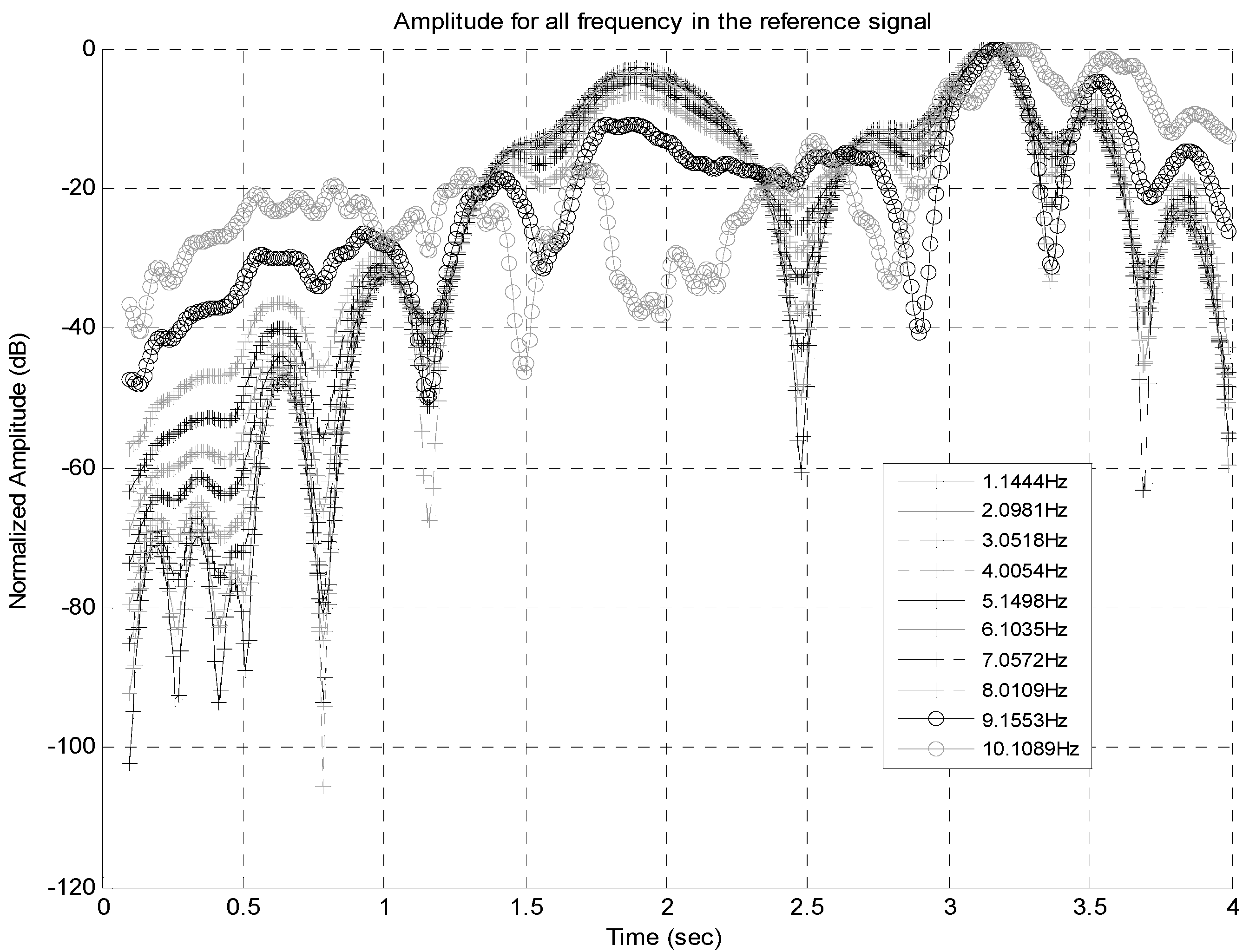
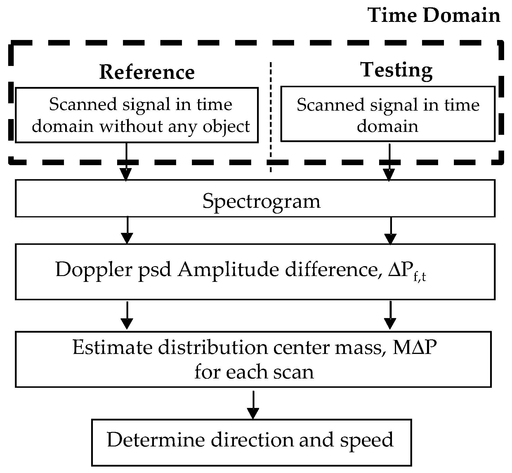
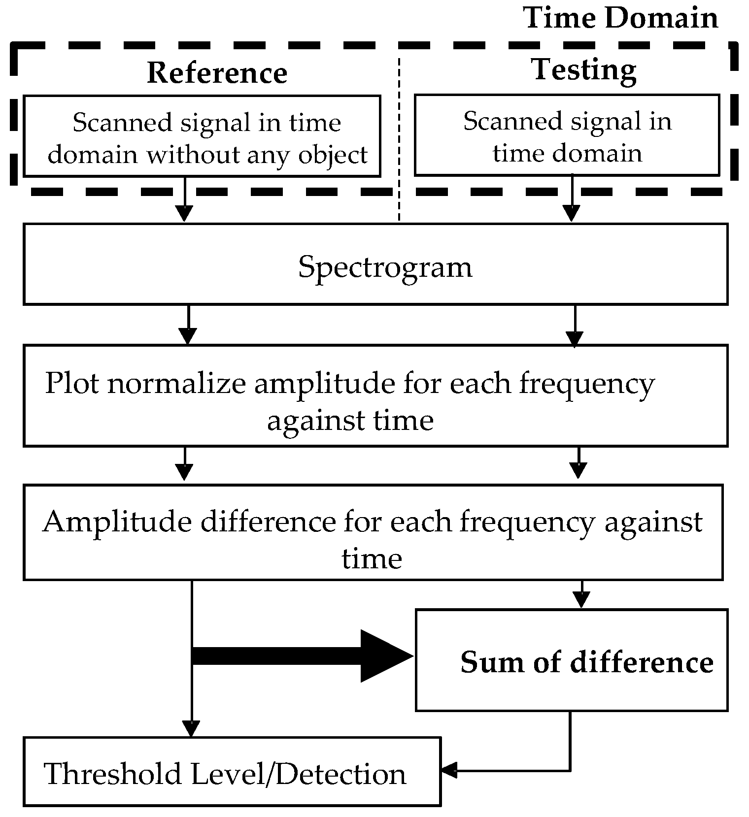
4. Joint T-F-Based Target Detection and Localization

This section describes the target detection and localization processing scheme in the FSR system with the rotational transmitter. Target detection based on the time domain signal is difficult, and the position information is not available (Figure 7a). Thus, an extended detection technique based on the joint time-frequency representation of the signal is proposed as depicted in Figure 8. The first step is converting the received signal for each complete scan cell into the T-F domain. Then, the normalized amplitude for each frequency is plotted against scanning time. The amplitude difference for each frequency between the scanned Doppler and the reference Doppler is calculated in this procedure. The last step is summing up the amplitude differences and plotting them with respect to time. Then, the detection threshold can be derived from this final plot.

Figure 9 shows the normalized amplitude of each received frequency extracted from the joint T-F representation of the signal. It is clearly shown that each frequency has a different amplitude along the scanning time. The peak of the normalized amplitude that happened at around 3.2 s shows that all Doppler frequencies possess a high amplitude for this time duration. The graph also shows that there are 10 significant Doppler frequencies in the received signal. It is important to treat each frequency independently for detection and localization as explained earlier due to the effect of Doppler shift.

Practically, for target detection in the proposed system, two considerations should be taken into account: (i) the receiver received a 3D forward scatter RCS lobe from the target and (ii) each time cell comprises many scattered points within the same vertical resolution cell. The different scattered points produce different shifted frequencies (f₁, f₂, … f_i) as shown in Figure 6a. Many scattered points are within the same time cell, T. This effect is crucial even for a small movement. Hence, the equation of the received Doppler signal (Equation (24)) is modified as follows:

$${\mathrm{f}}_{\mathrm{sc}\_\mathrm{ri}}(\mathrm{t})=\frac{{\mathrm{rTx}}_{\mathsf{\omega }}}{\lambda }\cos \left(\left[{\cos }^{-1}\left(\frac{{\mathrm{Obj}}_{\mathrm{xi}}-{\mathrm{Tx}}_{\mathrm{x}}}{\sqrt{{\left({\mathrm{Tx}}_{\mathrm{x}}-{\mathrm{Obj}}_{\mathrm{xi}}\right)}^2+{\left({\mathrm{Tx}}_{\mathrm{y}}-{\mathrm{Obj}}_{\mathrm{yi}}\right)}^2}}\right)\right]-\mathsf{\phi }\right)\cos \left(\pi -ta{n}^{-1}\left(\frac{{\mathrm{Obj}}_{\mathrm{yi}}-{\mathrm{Rx}}_{\mathrm{y}}}{{\mathrm{Obj}}_{\mathrm{xi}}-{\mathrm{Rx}}_{\mathrm{x}}}\right)-{\mathsf{\Omega }}_1\right)$$

(30)

where i shows the number of scattered point.

The novel detection technique in this paper utilizes the sum of differences in amplitude for each frequency content, A_s(T), in the signal along the sweep time. The target is detected if the sum of the difference between signal from a target and reference signal is greater than the threshold. The sum of the difference in amplitude for each frequency content is given by:

$${\mathrm{A}}_{\mathrm{s}}\left(\mathrm{T}\right)={\displaystyle \sum }_{\mathrm{i}=1}^{\mathrm{i}=\mathrm{n}}∆{\mathrm{f}}_{\mathrm{i}}\left(\mathrm{T}\right)={\displaystyle \sum }_{\mathrm{i}=1}^{\mathrm{i}=\mathrm{n}}{\mathrm{f}}_{\mathrm{sc}\_\mathrm{ri}}(\mathrm{T})-{\mathrm{f}}_{\mathrm{dr}\_\mathrm{ri}}\left(\mathrm{T}\right)$$

(31)

where T = 1, 2…J, and J is determined by the number of signals and the length of the window. ∆f_i is the difference in the amplitude for frequency I, and f_{dr_ri} is the amplitude of reference signal at frequency i.

Good statistics are required to decide the threshold level for the reference signal. The threshold is defined by the sum of the difference in amplitude for each frequency content for all signals during the mapping clutter from the ground, as shown in Figure 10. From the analysis, the detection threshold level (difference) of 3 dB is chosen. It has to be clarified here that the detection threshold level might be different for different areas, and it has to be adaptive. Hence, many background clutter signals need to be collected to be an optimum reference signal.

The adaptive Constant False Alarm Rate (CFAR) processing is an important procedure for producing precise target images separated from the existing clutter. Then, the extracted target signatures that are free of clutter can be used to estimate different target parameters for their classifications. Therefore, a modified CFAR technique has to be made by using the information of A_s(T). In CFAR, the term ‘Cell Under Test’ (CUT) is commonly used for the cell to be detected, and in this paper, CUT will be assumed as the signal at frequency i.

The threshold, $\mathrm{Th}$, is determined after estimating the average A_s(T) from the neighboring cells and is given by:

$$\mathrm{Th}=\mathsf{\epsilon }{\mathrm{P}}_{\mathrm{n}}$$

(32)

where ε is the scaling factor (threshold factor) and $P_n$ is the estimated amplitude difference, ∆f_i.

The cell-averaging CFAR detector is used, where the noise samples are extracted from the training cells (leading and lagging cells) around the CUT (the signal with frequency i). The estimated noise can be calculated by the following [21].

$${\mathrm{P}}_{\mathrm{n}}=\frac{1}{\mathrm{I}}{\displaystyle \sum }_{\mathrm{i}=1}^{\mathrm{I}}{\mathrm{x}}_{\mathrm{i}}$$

(33)

where x_i is the sample in each training cell (i.e., each frequency content) and I is the number of training cells (i.e., number of frequencies). The number of leading cells is generally the same as the lagging ones. To avoid having a leaked signal component in the training cell, which may have a harmful effect on the noise estimation, guard cells leading and lagging the CUT are used.

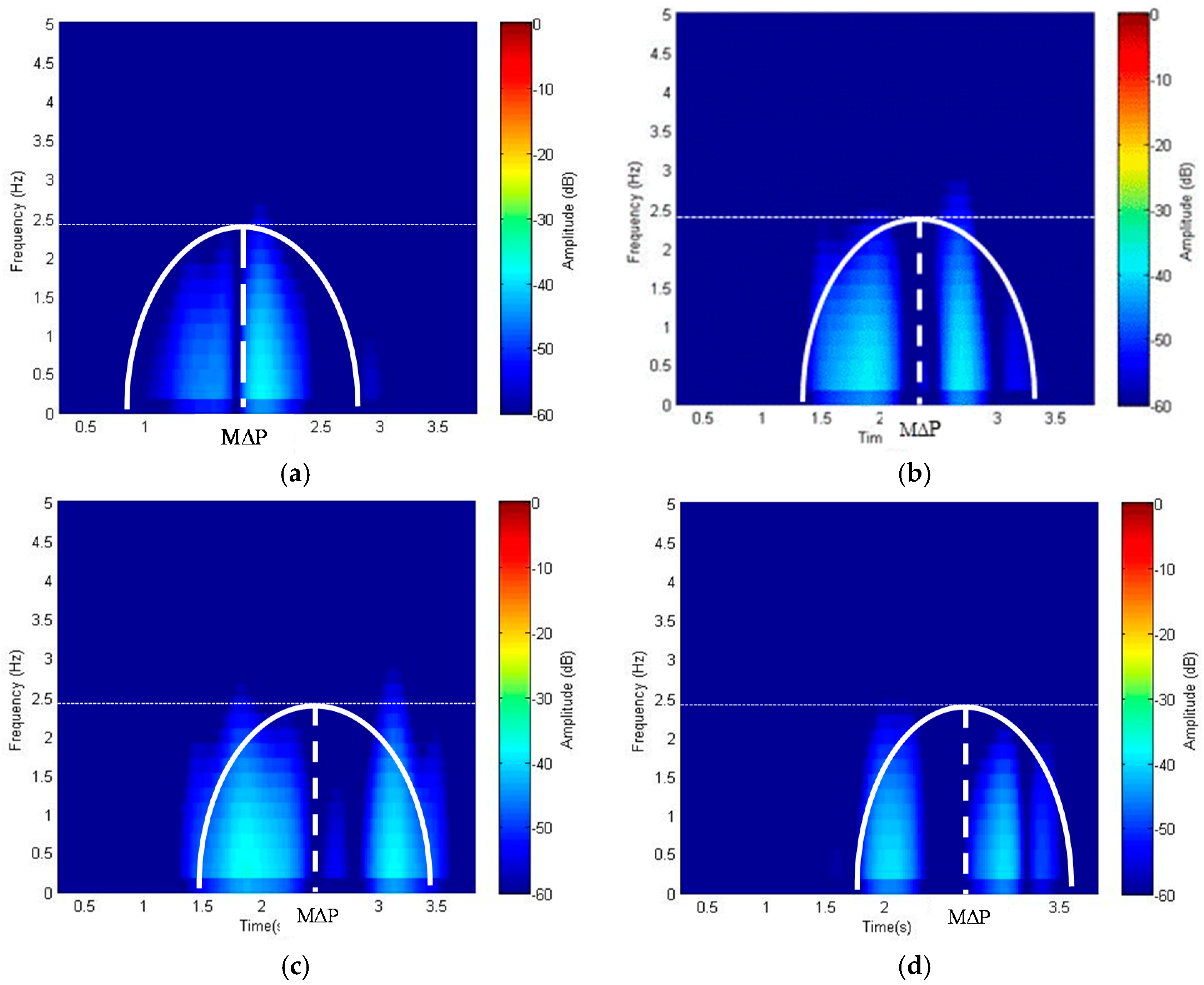
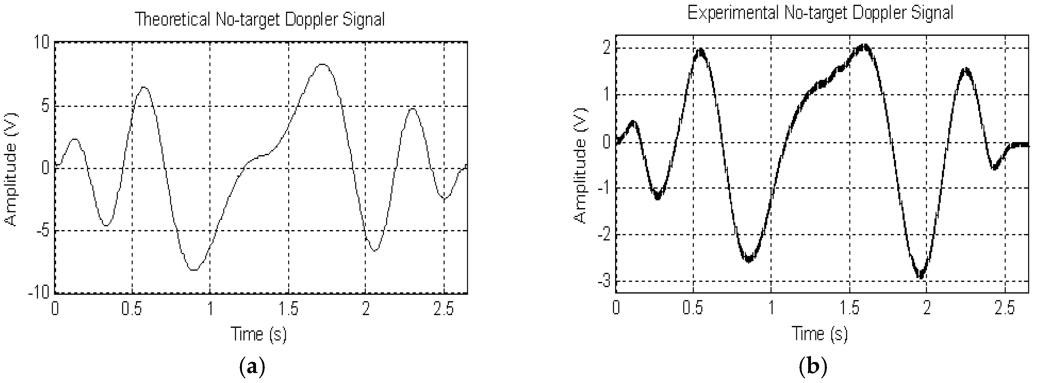
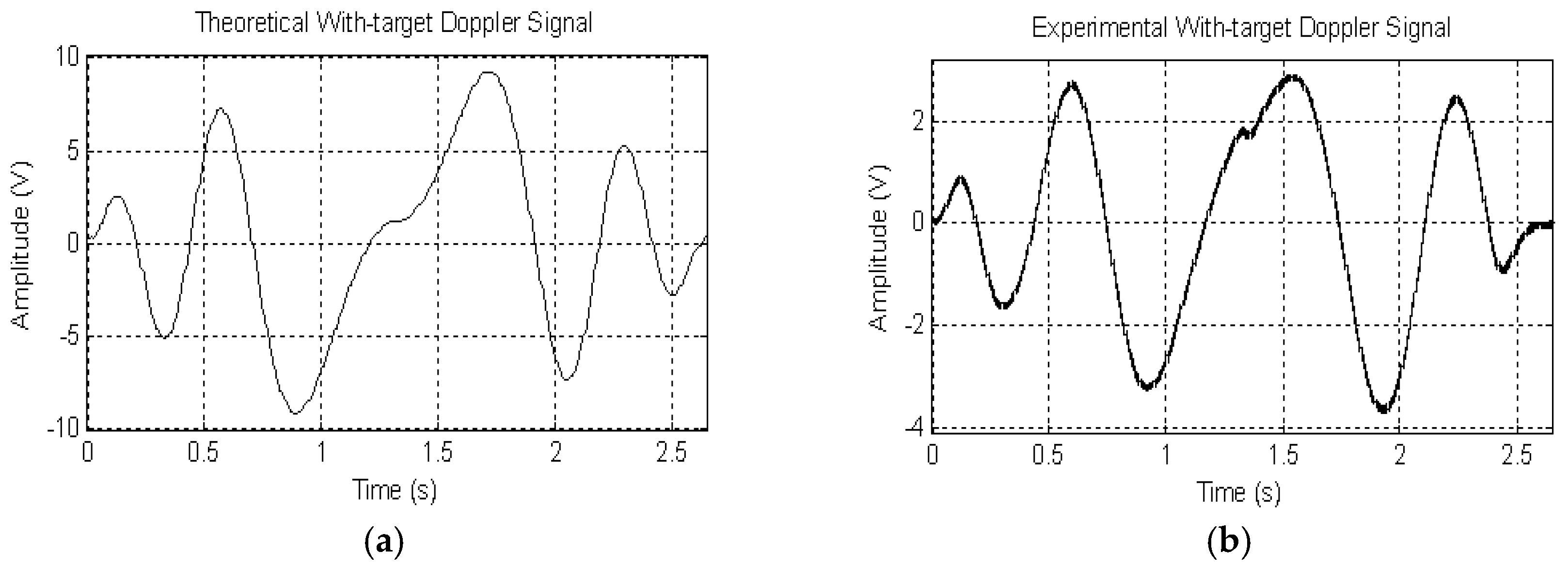
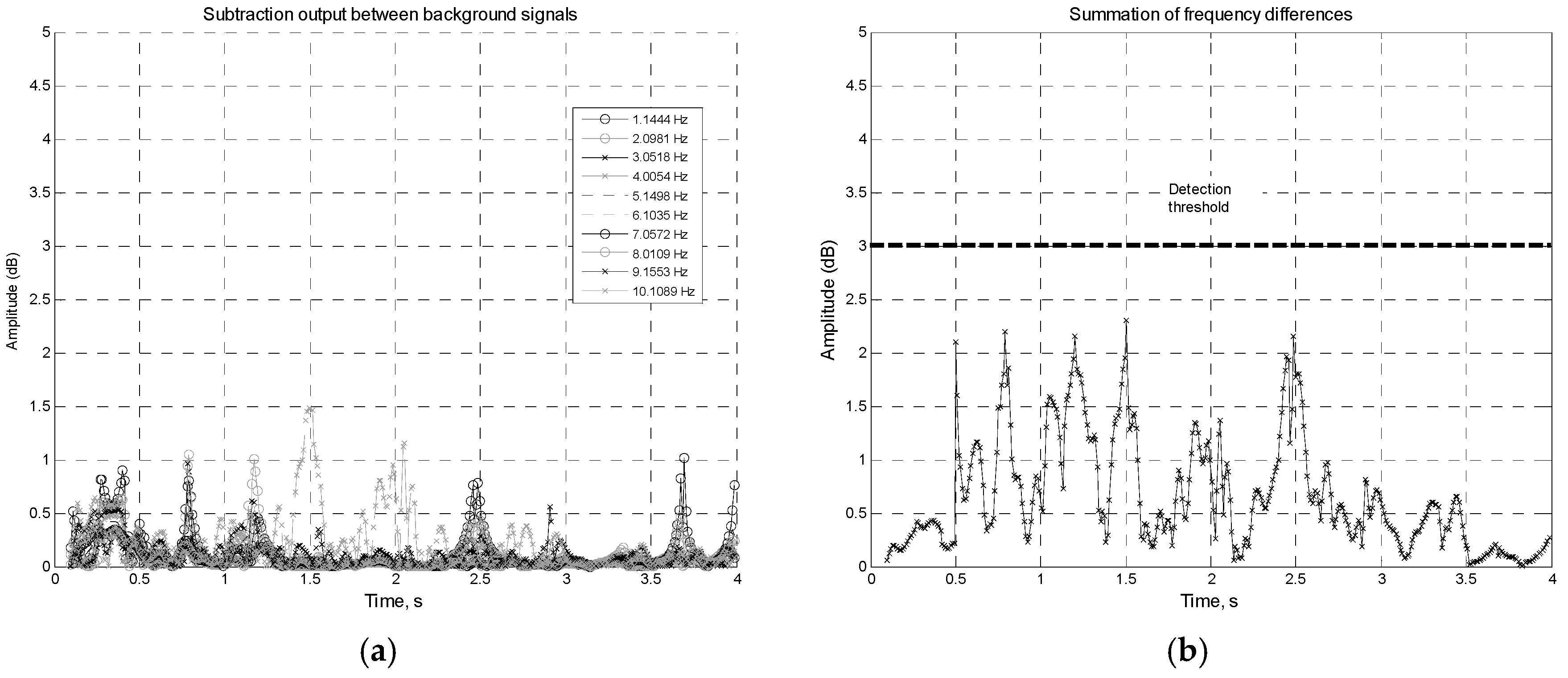
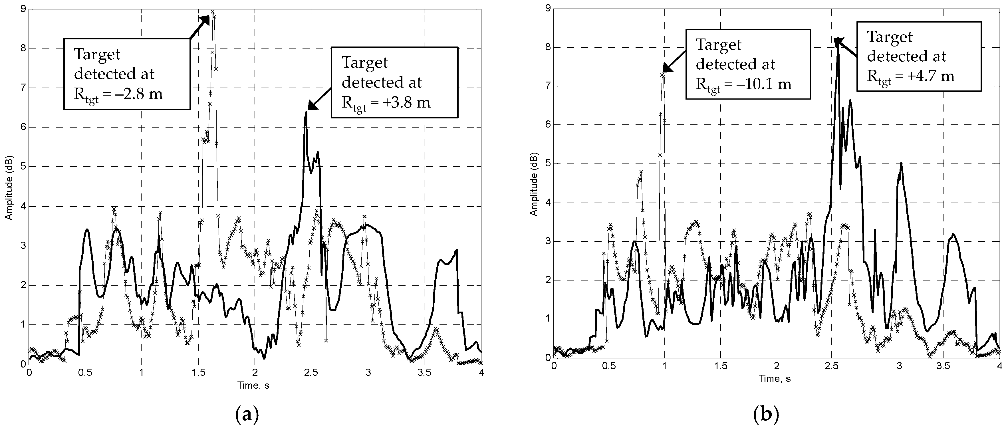
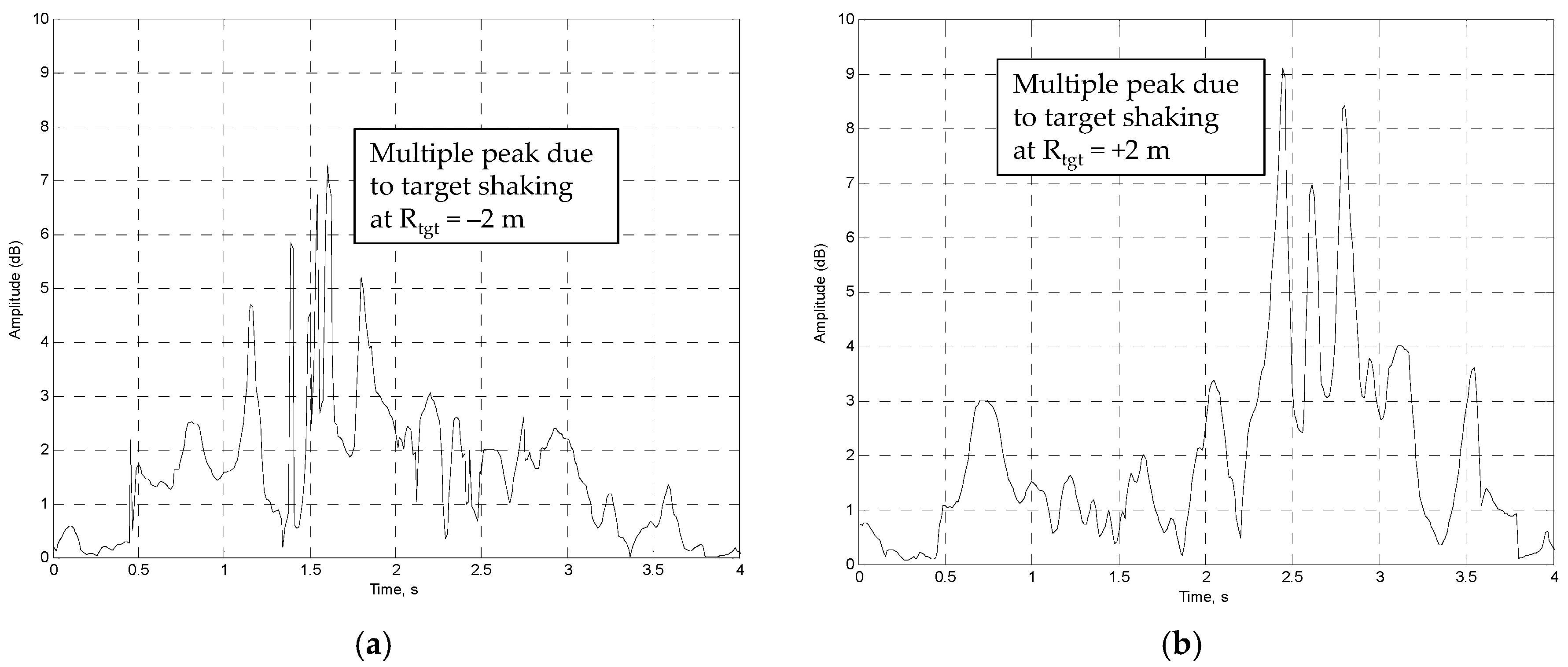
4.1. Stationary Target Detection and Localization

Two conditions as explained in Section 3 for detecting (i) target sitting and (ii) slight shaking were tested. The sum of the differences in amplitude for each frequency, A_s, was calculated for each set for target detection and localization. Figure 11a,b shows the plot of the final output of A_s, for a target sitting in a static position at R_tgt = +2 m, −2 m and R_tgt = +4 m, 4 m, respectively, with R_b = 10 m. Note that the experiment was done separately; the figures combine the results for illustrative purposes. The peak of summation differences is obvious even for a target sitting in completely stationary mode. The target is clearly detected by the peak of the amplitude, which is way above the 3-dB threshold. The highest peak of A_s is used for target detection, although some peaks at different times appeared to be more than the threshold. Target location, R_tgt, can be estimated by calculating the transmitter antenna looking angle, θ1 (Figure 2), for each scan. The angle θ1 can be determined from the time position of the peak As; for example, Figure 11a shows peak As at ts = 1.65 s; thus, θ₁ = 15.75°. The target localization result is tabulated in

Table 2. Target detection result from the proposed FSR system compared to the actual position.

Actual Position, Rtgt from FSR Baseline, (m)	Antenna Look Angle, θ1 = (ts/Trot)×180°	Estimated Rtgt from As (m) Rtgt = Rb × tan(90° − θ1)
−2	15.75°	−2.82
+2	20.81°	+3.8
−4	45.28°	−10.1
+4	25.17°	+4.7

, the negative and positive signs indicating the target to the left and right of the FSR baseline, respectively. The results in Table 2 highlight some offset in location, especially for a target that is supposed to be at −4 m from the FSR baseline. This could be explained due to the wide antenna beam width used during the experiment. Another factor is the precision of the motor that holds the transmitting antenna. The antenna rotates in the clockwise direction and produced a small vibration on the rotating arm (that holds the antenna) at the beginning. The vibration form the rotating arm effects the received Doppler frequency, and it became severe for a high vibration rate. Thus, the target located within the starting area of the antenna was detected with poor precision, in this case the target at −4 m (Figure 11b). The target location, R_tgt, precision is high when the target is near to the baseline and towards the end of the scanning area. Although the system’s resolution is not dealt with in this paper, it can be improved by employing a small antenna beam width, like a pencil beam shape, and using a rotating system with high stability.

In the case of the target sitting with slight shaking, the ripple of the Doppler shift frequency is detected as depicted in Figure 12. This is due to Doppler scattered from other shaking parts, like arms, knees, etc. Multiple peaks of amplitude can be seen clearly at the area of the target’s shaking. Multiple peaks occurred due to the rapid rate of change of the total path length travelled signal between the transmitter and receiver induced by body shaking. The rest of the signal, which is below the 3-dB threshold, comes from the clutter.

The difference between the target for Conditions i and ii can be summarized as the target with slight movement creates multiple ripples of As. Those peaks appeared above the 3-dB threshold level, which is the sign of target existence. Apart from the micro Doppler effect explained earlier, multiple peaks of amplitude occur with the slight movement due to the variation of the received amplitude at different frequencies. The system manages to differentiate between the target sitting completely stationary and the target sitting with slight movement.

4.2. Moving Target Detection and Localization

This section discusses the proposed detection scheme for the moving target crossing the middle of the FSR baseline (R_cross = 10 m). The target moved in the crawling condition, which resembles the low profile intruder scenario. If the signal processing scheme described in Figure 8 is applied to this scenario, it may produces multiple spikes scattered from many moving points. Confusion that might lead to misinformation, such as the number of targets and the direction of the target, may arise. An improved detection scheme based on the different power spectral density magnitude of the signal’s joint T-F is recommended, and it is discussed below.

As stated earlier, the aim of this stage was to scrutinize the feasibility of the proposed FSR with the rotational transmitter for security surveillance; hence, the complexity in signal processing is minimized. The task is to monitor the change in the received signal due to the target movement on the ground surface. An established method, such as Coherent Change Detection (CCD), was proposed for surface displacement monitoring as applied in SAR [22,23,24]. The CCD technique correlates consecutive SAR images at the phase level and relates the phase changes to the actual surface change. However, the integration of the CCD concept with FSR is a new idea, and therefore, appropriate consideration has to be made. Firstly, the received signal in FSR does not carry any phase information; thus, the coherent detection scheme is not used. Moreover, the image that needs to be processed is the signal in joint T-F representation, which is opposed to the SAR image in CCD.

Consequently, a modified version of CCD, which is based on the change detection of the amplitude of the Doppler power spectrum density (D-psd), is suggested. Figure 13 shows the detection signal processing scheme for the moving target. Again, the background signal is taken as a reference. After converting the signal into the joint T-F representation, the amplitude of D-psd is calculated. Let the D-psd amplitude of the reference signal be Pr_f,t and the D-psd for the newly-scanned signal be Pz_f,t. Then, the amplitude difference of D-psd is given by:

∆P_f,t = Pr_f,t − Pz_f,t

(34)

where f and t indicate the frequency and time, respectively. Figure 14 shows the plot of ∆P_f,t for low profile target crawling crossing the FSR baseline for four consecutive scanned durations. Once the target slowly enters the FSR baseline, there is a significant change in amplitude D-psd as produced by ∆P_f,t. The distribution center mass, M∆P, for each scan is determined and used as the reference point. The target trajectory can be predicted by analyzing the change in M∆P (Figure 14a–d; in this case, the target crawls from left to right). M∆P can be determined by using the best fit curved to get the envelope for ∆P_f,t. Then, the middle point of the mass distribution is selected as the M∆P. Moreover, the target speed can also be estimated by utilizing the time difference of M∆P for every revisit time. Since the time position of M∆P and antenna looking angle, θ1 (Figure 2), for each scan are known, thus the target speed can be calculated and is given in

Table 3. Result for the target detection and the target’s speed by using ∆M∆P.

	Scan i	Scan ii		Scan iii		Scan iv
M∆P (s)	1.96	6.31		10.47		14.6
Antenna look angle, θ1 ${\mathsf{\theta }}_1=\left(\frac{\mathrm{M}∆\mathrm{P}}{{\mathrm{T}}_{\mathrm{rot}}}\right)\times {180}^{°}$, (Trot = 4 s)	88.2°	103.95°		111.15°		117°
Distance from baseline Rtgt (m) Rtgt = Rcross × tan(90°–θ1) for M∆P < 2 s Rcross × tan(θ1–90°) for M∆P > 2 s	−0.314	+2.484		+3.869		+5.095
∆M∆P (s) (M∆Pscann − M∆Pscann−1)	4.35		4.16		4.13
Speed (m/s)	0.63		0.34		0.30
Average speed	0.42 m/s (misclassified by 0.8 m/s)

n, number of scans.

. Actual target moving speed was 0.5 m/s, which is slightly higher than the estimated one, and the target moves from the left side to the right side of the transmitter, as captured by the proposed scheme.

5. Conclusions

Forward scattering radar has been discussed for target detection, tracking and classification with applications to air, ground and maritime environments. Although research and development in FSR has gained interest for almost a decade, mostly fixed transmitters are used to send the signal. Thus, the work presented in this paper explored and showed the capability of the FSR system with a rotational transmitter to scan the area of interest and detect a stationary or slow-moving target, which is very difficult for the conventional FSR system to detect. Practical applications for detecting a low profile, almost stationary intruder and intruder crawling have been tested. A novel signal processing detection scheme based on the joint T-F domain of the received signal is integrated with the proposed FSR system. As a result, a stationary target and a slow-moving target crossing the FRS baseline were detected for different locations and modes. The main advantage of using the FSR system with the rotational transmitter is the degree of freedom it possesses in controlling the Doppler frequency at the receiver, consequently allowing low profile target detection. Hence, the paper has shown the system’s potential for remote security and border surveillance. Based on the previous work, fixed FSR had shown that target detection and classification are affected by the target’s speed. However, this paper suggests that the transmitter is rotating, and the rotational speed can be controlled and optimized. Thus, the effect of rotational speed on the system sensitivity is interesting, and it will be analyzed in the future. The resolution is not discussed in this paper; however, the resolution can be further increased by using a narrow antenna beam width and pulse signal, which is also a subject for future work. In addition, the FSR coverage can be increased by using a network of distributed receivers. Interestingly, the concept of the rotational transmitter in FSR can be further explored for moving target detection, tracking and classification with a multisite receiver system.

References

1. Cherniakov, M. Bistatic Radar: Principles and Practice, 1st ed.; John Wiley & Sons: Chichester, UK, 2007. [Google Scholar]
2. Glaser, J. Forward Scatter Radar for Future Systems. WSTIAC Q. 2011, 10, 3–8. [Google Scholar]
3. Skolnik, M.I. Radar Handbook, 2nd ed.; McGraw-Hill Professional: New York, NY, USA, 1989. [Google Scholar]
4. Blyakhman, A.B.; Runover, I.A. Forward scattering radiolocation, bistatic RCS and target detection. In Proceedings of the 11th IEEE/AESS Radar Conference on Radar into the Next Millennium, Waltham, MA, USA, 20–22 April 1999.
5. Blyakhman, A.B.; Myakinkov, A.V.; Ryndyk, A.G. Measurement of target coordinates in three-dimensional bistatic forward-scattering radar. J. Commun. Technol. Electron. 2006, 51, 397–402. [Google Scholar] [CrossRef]
6. Chapurskiy, V.V.; Sablin, V.N. SISAR: Shadow inverse synthetic aperture radiolocation. In Proceedings of the Record of the IEEE 2000 International Radar Conference, Alexandria, VA, USA, 7–12 May 2000.
7. Cherniakov, M.; Abdullah, R.R.; Jancovic, P.; Salous, M.; Chapursky, V. Automatic ground target classification using forward scattering radar. IET Proc. Radar Sonar Navig. 2006, 153, 427–437. [Google Scholar] [CrossRef]
8. Raja Abdullah, R.S.A.; Rasid, M.F.A.; Mohamed, M.K.H. Improvement in detection with forward scattering radar. Sci. China Inf. Sci. 2011, 54, 2660–2672. [Google Scholar] [CrossRef]
9. Hassan Mohamed, M.K.; Cherniakov, M.; Rasid, M.F.A.; Raja Abdullah, R.S.A. Automatic Target detection using wavelet technique in forward scattering radar. In Proceedings of the EuRAD 2008, Amsterdam, The Netherlands, 30–31 October 2008.
10. Hu, C.; Sizov, V.; Antoniou, M.; Gashinova, M.; Cherniakov, M. Optimal signal processing in ground-based forward scatter micro radars. IEEE Trans. Aerosp. Electron. Syst. 2012, 48, 3006–3026. [Google Scholar] [CrossRef]
11. Daniel, L.; Gashinova, M.; Cherniakov, M. Maritime target cross section estimation for an UWB FSR network. In Proceedings of the EuRAD 2008, Amsterdam, The Netherlands, 30–31 October 2008.
12. Hristo, K.; Vera, B.; Ivan, G.; Dorina, K.; Liam, D.; Kalin, K.; Marina, G.; Mikhail, C. Experimental verification of maritime target parameter evaluation in forward scatter maritime radar. IET Radar Sonar Navig. 2015, 9, 355–363. [Google Scholar]
13. Gashinova, M.; Daniel, L.; Cherniakov, M.; Lombardo, P.; Pastina, D.; De Luca, A. Multistatic forward scatter radar for accurate motion parameters estimation of low-observable targets. In Proceedings of the International Radar Conference, Lille, France, 13–17 October 2014.
14. Abdullah, R.R.; Salah, A.A.; Aziz, N.A.; Rasid, N.A. Vehicle recognition analysis in LTE based forward scattering radar. In Proceedings of the IEEE Radar, Philadelphia, PA, USA, 2–6 May 2016.
15. Gashinova, M.; Daniel, L.; Hoare, E.; Sizov, V.; Kabakchiev, K.; Cherniakov, M. Signal characterisation and processing in the forward scatter mode of bistatic passive coherent location systems. EURASIP J. Adv. Signal Proc. 2013, 2013, 13–16. [Google Scholar] [CrossRef]
16. Abdullah, R.A.R.; Ali, A.M.; Rashid, N.E.A. Stationary object detection in forward scattering radar. In Proceedings of the IET Radar Conference, Hangzhou, China, 14–16 October 2015.
17. Martelli, T.; Colone, F.; Lombardo, P. First experimental results for a wifi-based passive forward scatter radar. In Proceedings of the 2016 IEEE Radar Conference (RadarConf), Philadelphia, PA, USA, 2–6 May 2016.
18. Gildas, K.; Christophe, B.; Philippe, P. Shadow radiation: Relations between Babinet principle and physical optics. In Proceedings of the 2014 IEEE Antennas and Propagation Society International Symposium (APSURSI), Memphis, TN, USA, 6–11 July 2014.
19. Glaser, J.I. Bistatic RCS of complex objects near forward scatter. IEEE Trans. Aerosp. Electron. Syst. 1985, 21, 70–78. [Google Scholar] [CrossRef]
20. Beasley, P. Tarsier\, a unique radar for helping to keep debris off airport runways. In Proceedings of the IET Seminar on the Future of Civil Radar, London, UK, 15 June 2006.
21. Radar, R.H. CFAR thresholding in clutter and multiple target situations. IEEE Trans. Aerosp. Electron. Syst. 1983, 19, 608–621. [Google Scholar]
22. Preiss, M.; Stacy, N.J.S. Coherent Change Detection: Theoretical Description and Experimental Results; Report No. DSTO-TR-1851; Defence Science and Technology Organisation: Salisbury, UK, 2006. [Google Scholar]
23. Ajadi, O.A.; Meyer, F.J.; Webley, P.W. Change detection in synthetic aperture radar images using a multiscale-driven approach geophysical institute. Remote Sens. 2016, 8. [Google Scholar] [CrossRef]
24. Antoniou, M.; Liu, F.; Zeng, Z.; Sizov, V.; Cherniakov, M. Coherent change detection using GNSS-based passive SAR: First experimental results. In Proceedings of the IET International Conference on Radar Systems (Radar 2012), Glasgow, UK, 22–25 October 2012.
Figure 1. Simplified conventional Forward Scattering Radar (FSR) geometrical topology and receiver system block diagram.
Remotesensing 08 01028 g001
Figure 2. FSR geometrical layout with the rotational transmitter for (a) the direct signal and (b) the signal scattered from the object.
Remotesensing 08 01028 g002
Figure 3. Antenna radiation pattern used for theoretical analysis and experimentayion (a) transmitter antenna and (b) receiver antenna.
Remotesensing 08 01028 g003
Figure 4. (a) Theoretical analysis of the no-target Doppler signal and (b) the received direct signal from the FSR system with the rotational transmitter.
Remotesensing 08 01028 g004
Figure 5. (a) Theoretical signal with a point target and (b) the received signal during the experiment from the direct and scattered signal from the object.
Remotesensing 08 01028 g005
Figure 6. (a) FSR experimental setup and geometrical scenario showing the motorized controlled rotational transmitter and fixed receiver; (b) target sitting in stationary and (c) target crawling crossing the FSR baseline.
Remotesensing 08 01028 g006
Figure 7. (a) Received signal comprised of the direct signal (Doppler from the transmitter and clutter) and received signal with target scattering; (b) spectrogram of the direct signal.
Remotesensing 08 01028 g007
Figure 8. Detection processing scheme based on the time-frequency (T-F) signal for the stationary signal.
Remotesensing 08 01028 g008
Figure 9. Normalized amplitude for each frequency along the scanning time.
Remotesensing 08 01028 g009
Figure 10. (a) Subtraction of the frequency’s normalized amplitude function and (b) the summation of the frequency difference of the reference (background) signals.
Remotesensing 08 01028 g010
Figure 11. Illustration of the experiment and plot of As for the target sitting in the static condition at the actual range from the baseline of (a) Rtgt = −2 m, +2 m and (b) Rtgt = −4 m, +4 m.
Remotesensing 08 01028 g011
Figure 12. Plot of As for a target sitting with slight shaking condition at the range from the baseline, Rtgt, of (a) −2 m and (b) +2 m.
Remotesensing 08 01028 g012
Figure 13. Detection and localization signal processing scheme for the moving target.
Remotesensing 08 01028 g013
Figure 14. Spectrogram of a target crawling and crossing the FSR baseline with the rotational transmitter at four different consecutive scanning times: (a) for Scan I; (b) for Scan ii; (c) for Scan iii; (d) for Scan iv.
Remotesensing 08 01028 g014