
Incremental and Enhanced Scanline-Based Segmentation Method for Surface Reconstruction of Sparse LiDAR Data


Abstract
:
1. Introduction
2. Related Work
3. Notations and System Overview
3.1. Notations
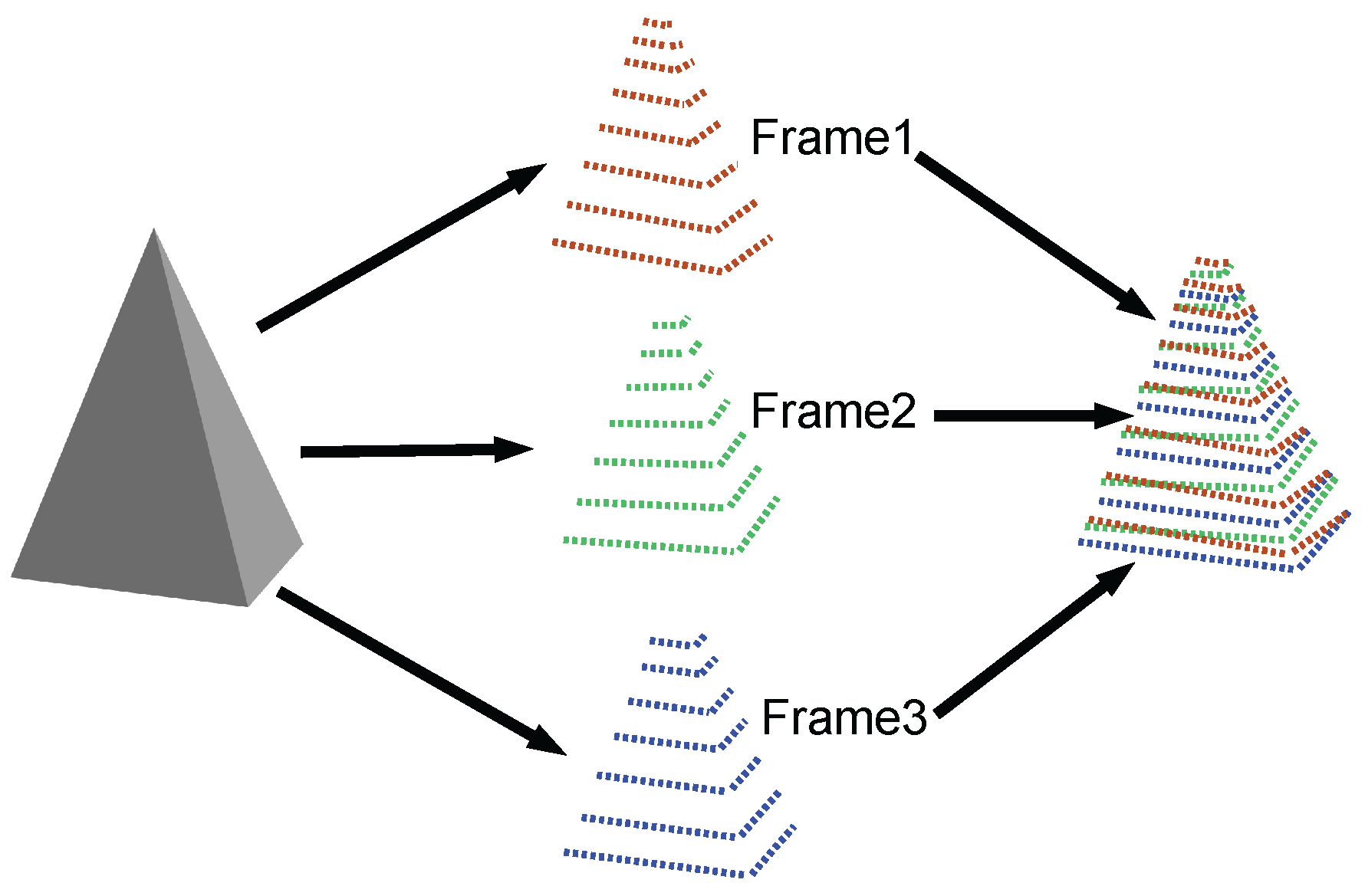
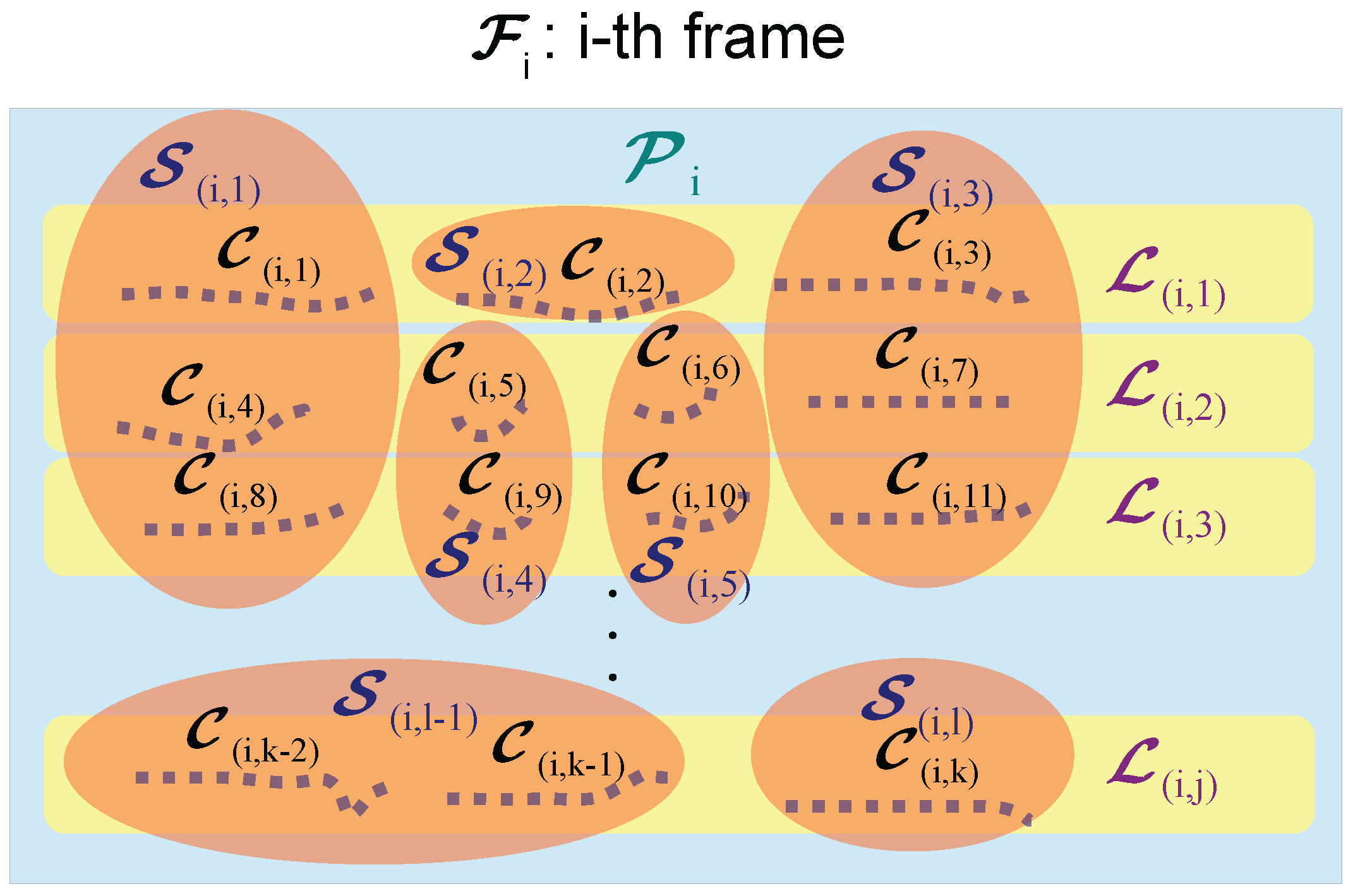
- A complete sweep by the LiDAR is denoted as one frame .
- The point cloud acquired in the i-th frame is denoted as .
- The scanline in is denoted as . In the case of Velodyne HDL-32, scanlines are {, , …, }.
- All the scanlines of are divided into several clusters line by line, denoted by {, , …, }.
- Clustered scanlines are then agglomerated into final segments {, , …, } of .
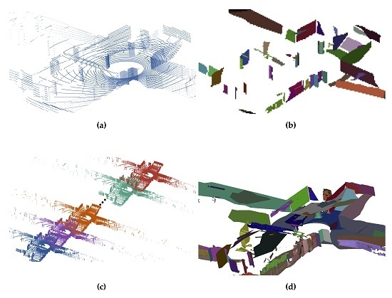
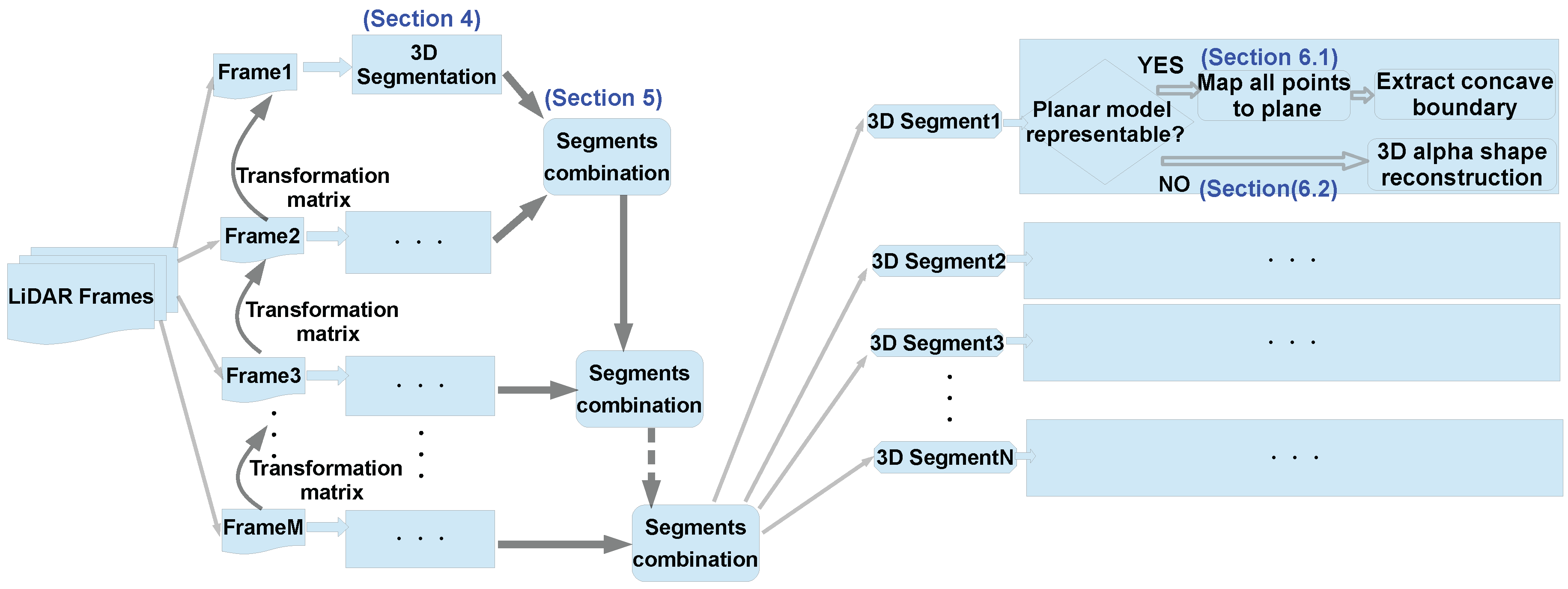
3.2. System Overview
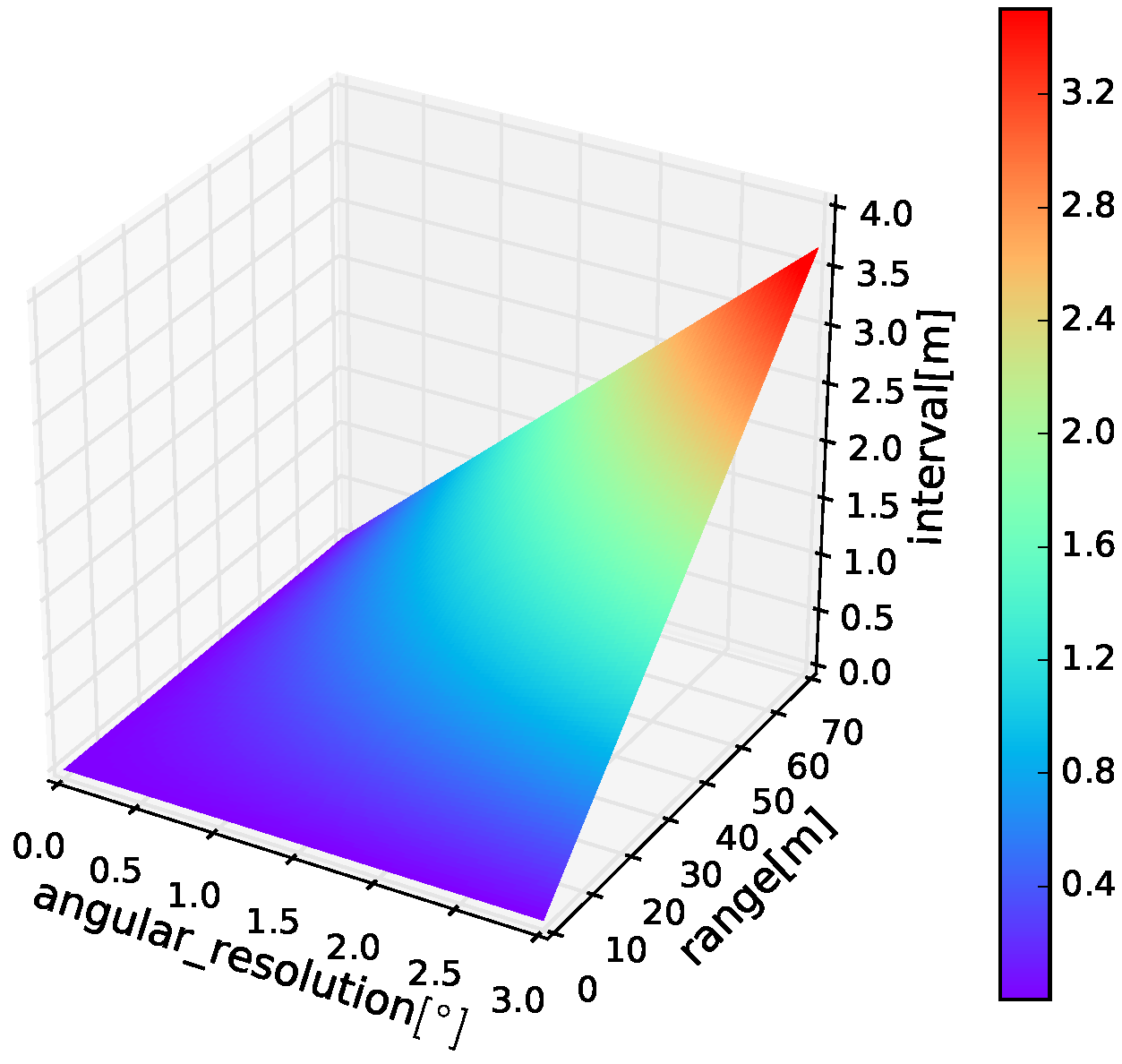
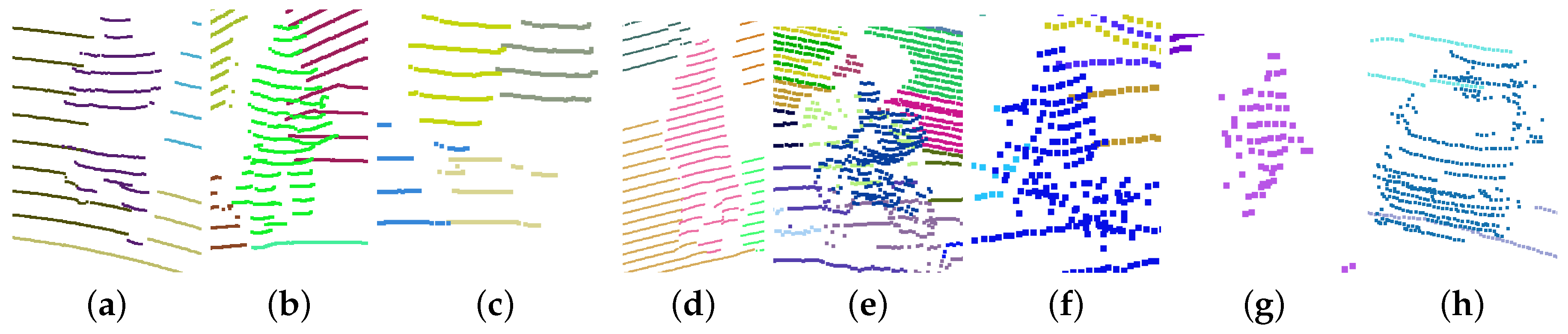
4. Scanline Continuity Constraint (SLCC) Segmentation
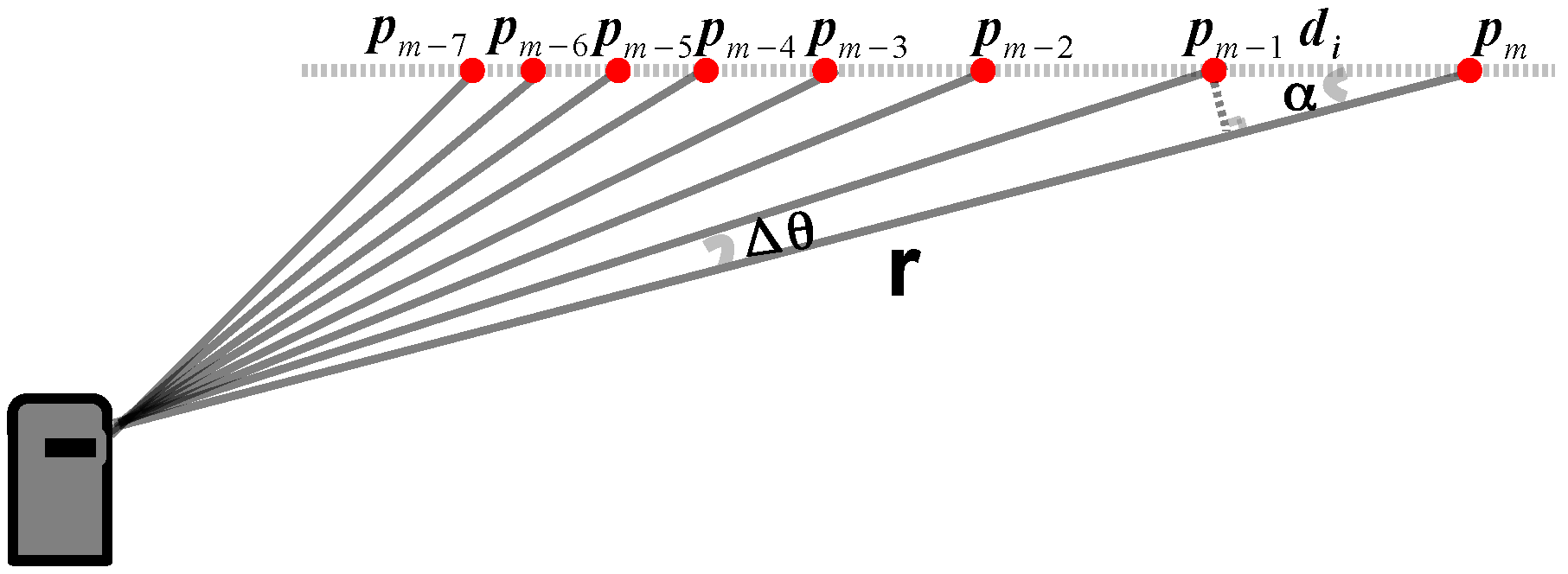
4.1. Clustering of Scanlines
| Algorithm 1: Scanline clustering |
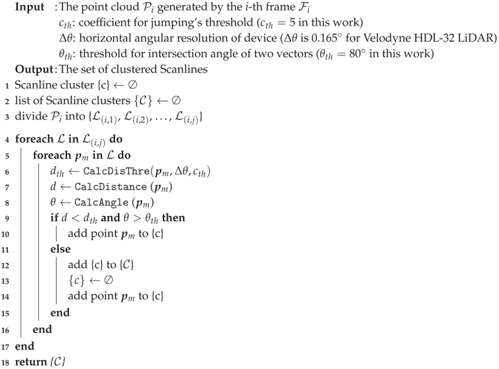 |
4.2. Agglomeration of Scanline Clusters
| Algorithm 2: Agglomeration of Scanline clusters |
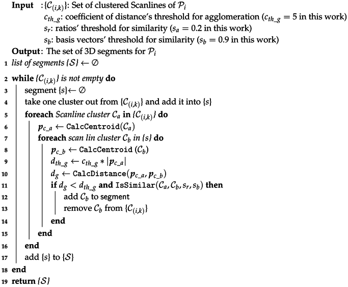 |
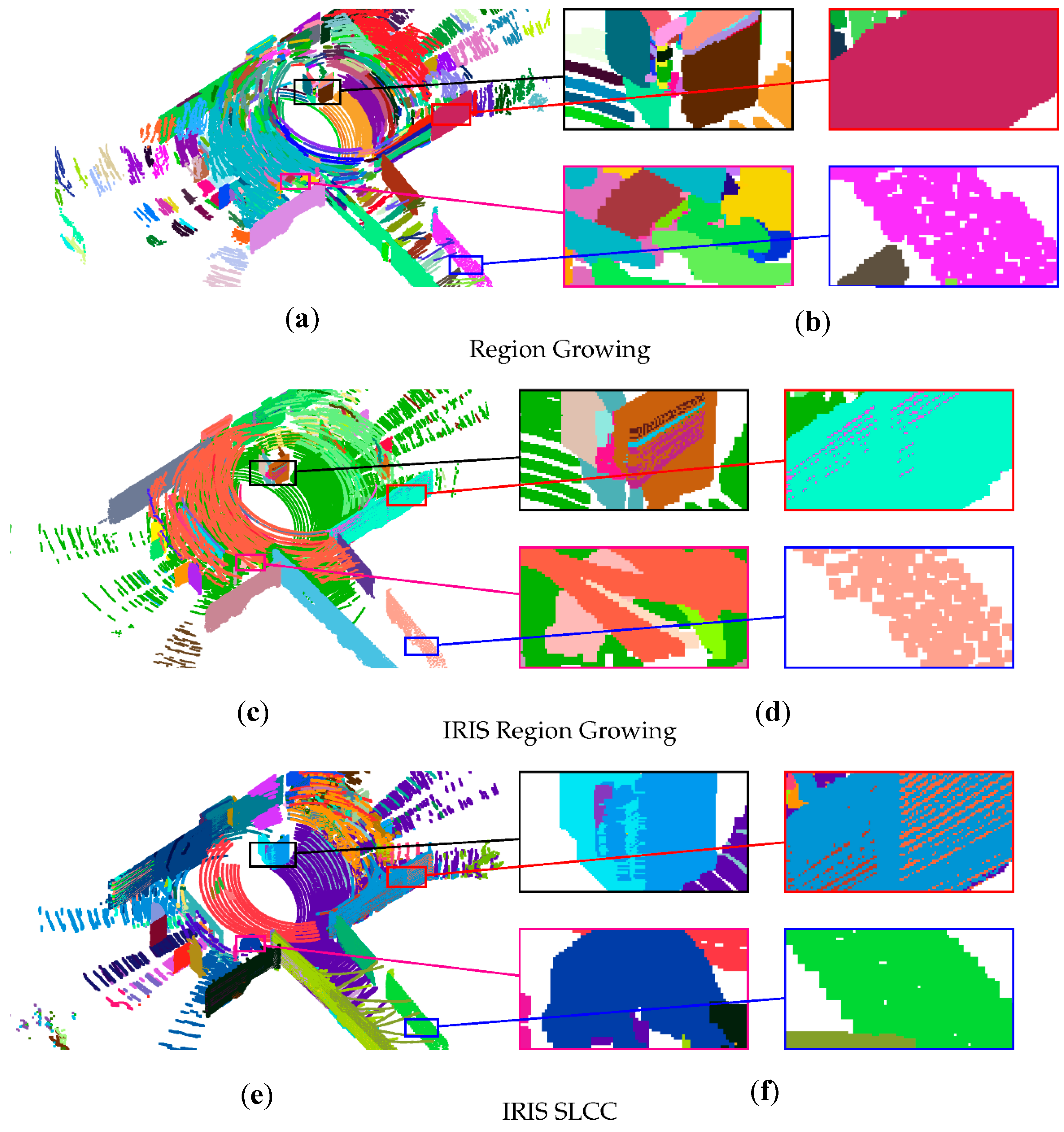
5. Incremental Recursive Segmentation (IRIS)
5.1. Combination of Segments from Different Point Clouds
5.2. Recursive Process for a More General Situation
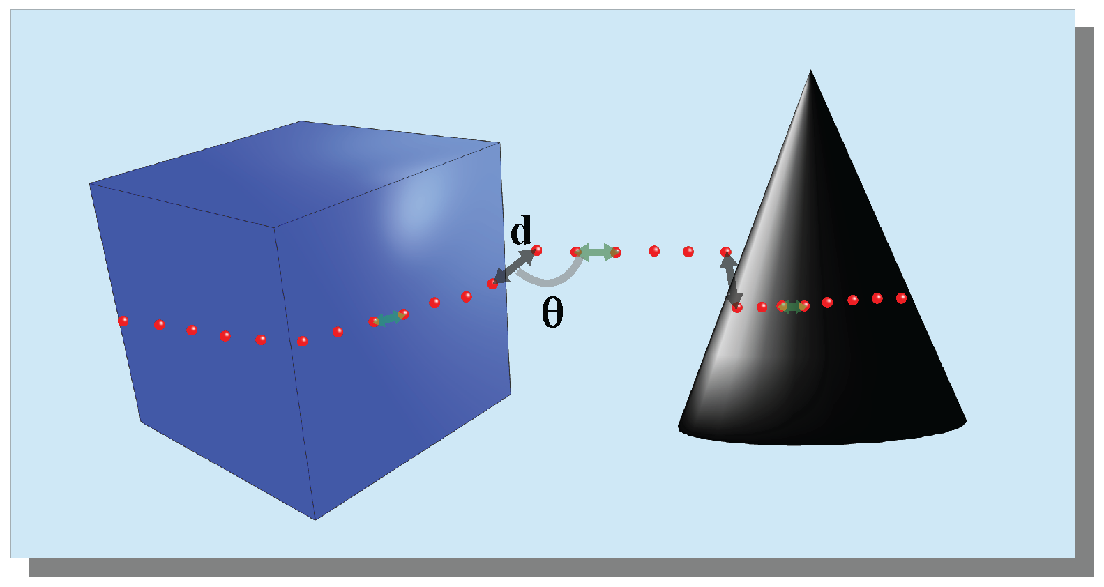
5.3. Similarity of 3D Segments
| Algorithm 3: Combine segments of two point clouds for IRIS |
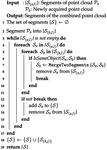 |
| Algorithm 4: IRIS |
 |
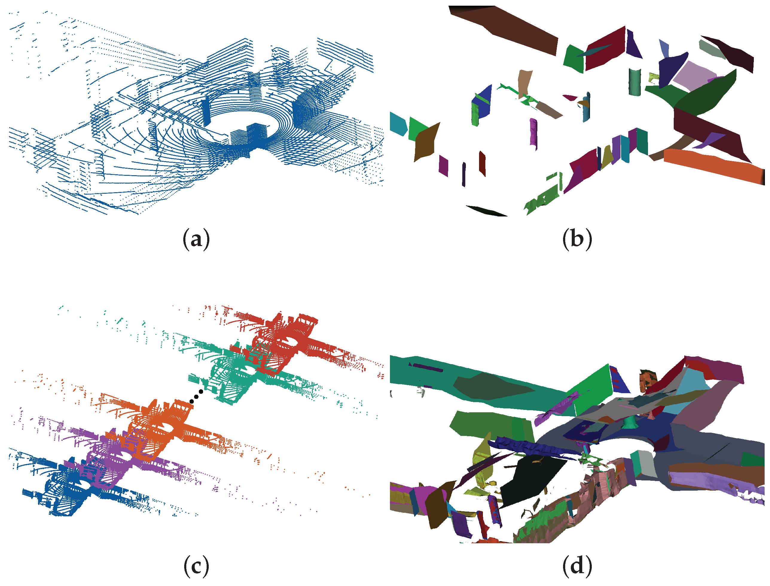
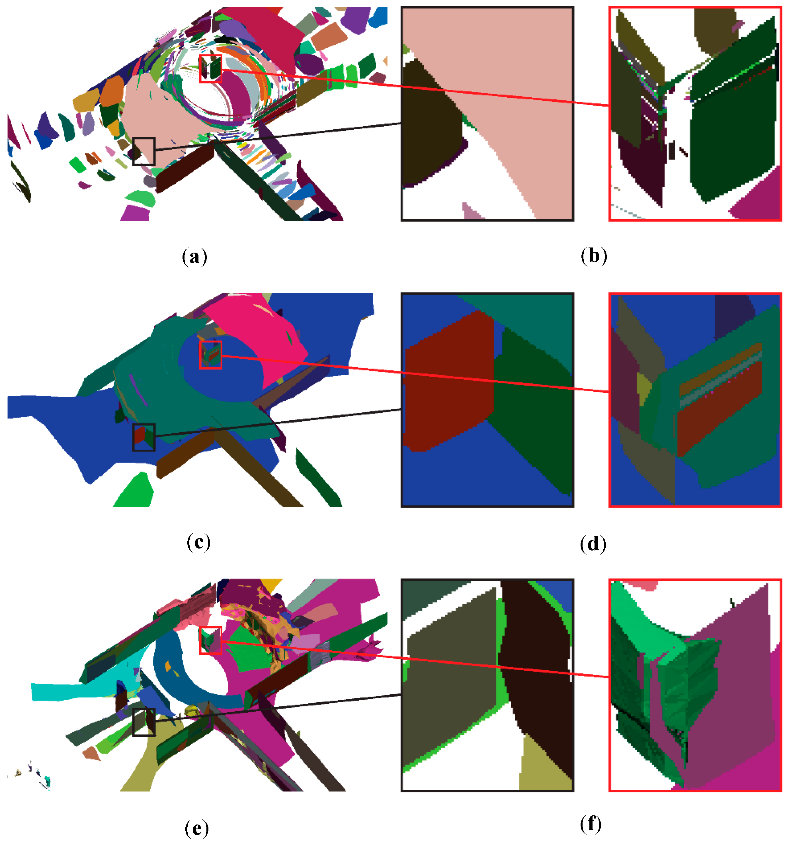
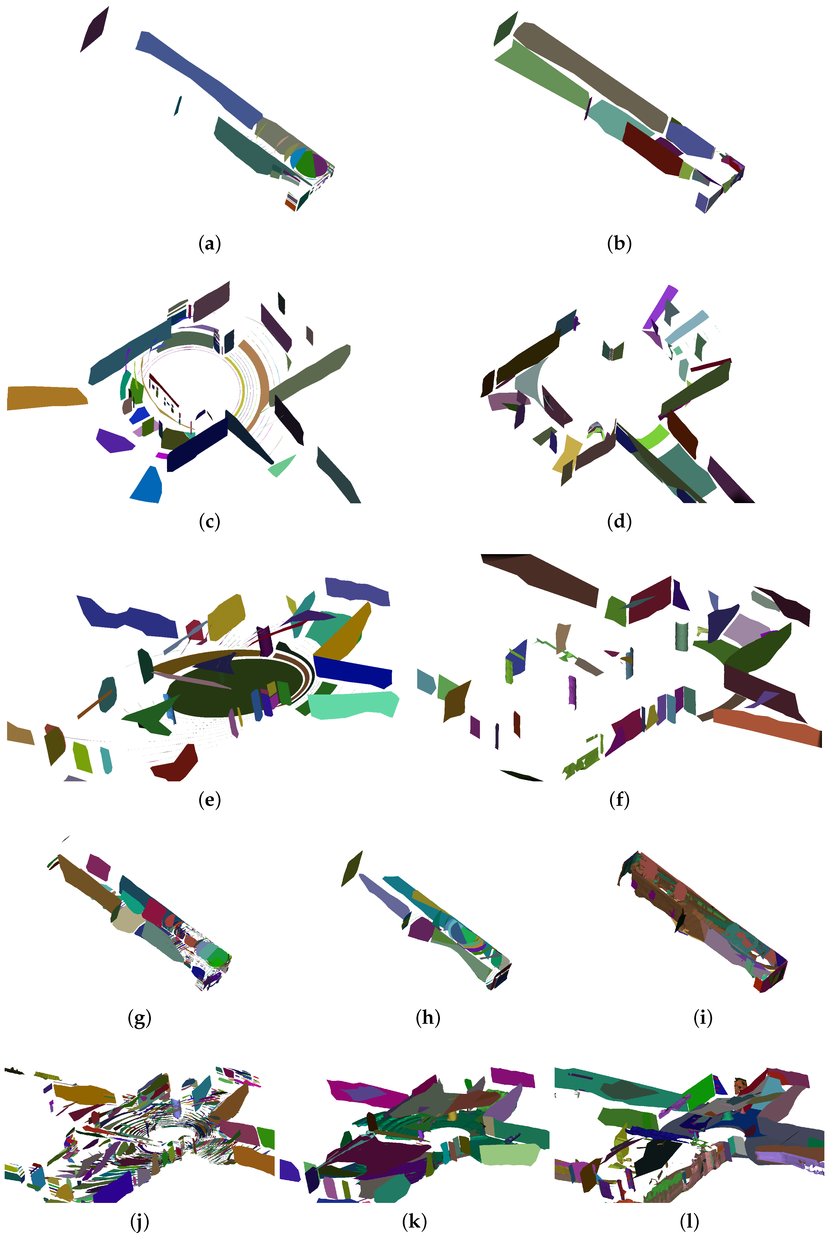
6. Surface Reconstruction
6.1. Planar Fitting and Polygon Boundary Extraction
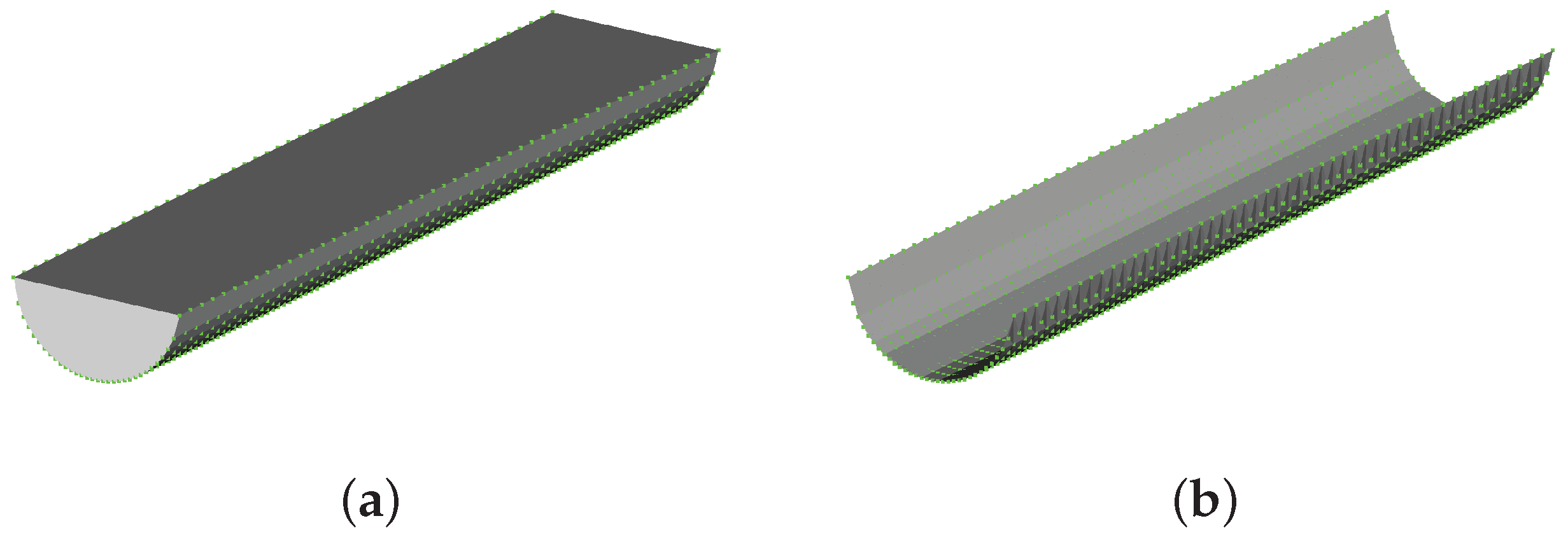
6.2. Surface Reconstruction for Non-Planar Shapes with Alpha Shape
7. Results and Discussion
7.1. Datasets
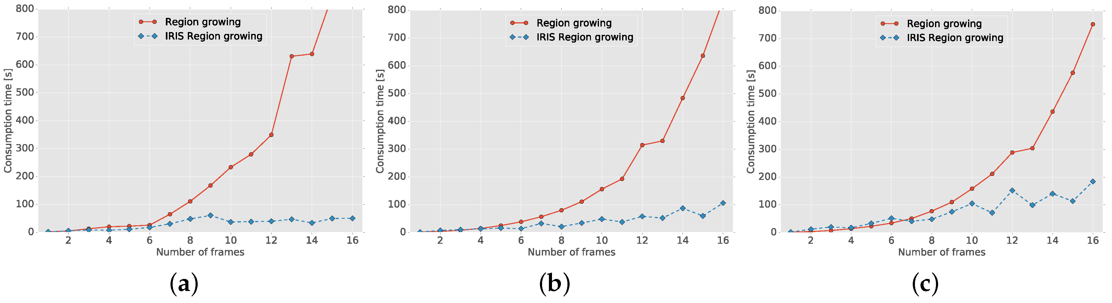
7.2. Time Performance of IRIS
7.3. Segmentation Performance
7.3.1. Scanlines Clustering
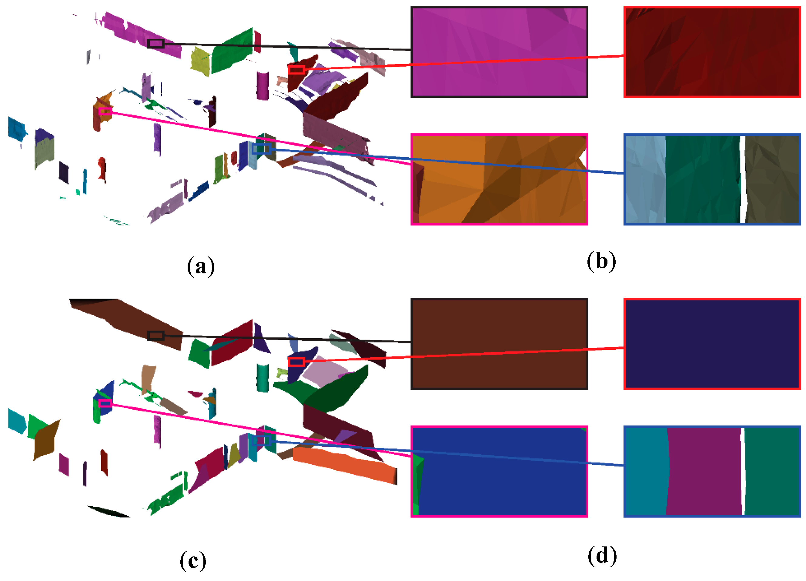
7.3.2. Segmentation
7.4. Surface Reconstruction
7.5. Limitations
8. Conclusions and Future Work
Author Contributions
Conflicts of Interest
References
- Nakagawa, M.; Kataoka, K.; Yamamoto, T.; Shiozaki, M.; Ohhashi, T. Panoramic rendering-based polygon extraction from indoor mobile LiDAR data. ISPRS Int. Arch. Photogramm. Remote Sens. Spat. Inf. Sci. 2014, 40, 181–186. [Google Scholar] [CrossRef]
- Previtali, M.; Barazzetti, L.; Brumana, R.; Scaioni, M. Towards automatic indoor reconstruction of cluttered building rooms from point clouds. ISPRS Ann. Photogramm. Remote Sens. Spat. Inf. Sci. 2014, 2, 281–288. [Google Scholar] [CrossRef]
- Rabbani, T.; van den Heuvel, F.A.; Vosselman, G. Segmentation of point clouds using smoothness constraint. ISPRS Int. Arch. Photogramm. Remote Sens. Spat. Inf. Sci. 2006, 36, 248–253. [Google Scholar]
- Fischler, M.A.; Bolles, R.C. Random Sample Consensus: A paradigm for model fitting with applications to image analysis and automated cartography. Commun. ACM 1981, 24, 381–395. [Google Scholar] [CrossRef]
- Rusu, R.B.; Cousins, S. 3D is here: Point Cloud Library (PCL). In Proceedings of the IEEE International Conference on Robotics and Automation, Shanghai, China, 9–13 May 2011.
- Grant, W.S.; Voorhies, R.C.; Itti, L. Finding planes in LiDAR point clouds for real-time registration. In Proceedings of the IEEE/RSJ International Conference on Intelligent Robots and Systems (IROS), Tokyo, Japan, 3–7 November 2013.
- Schnabel, R.; Wahl, R.; Klein, R. Efficient RANSAC for point-cloud shape detection. Comput. Graph. Forum 2007, 26, 214–226. [Google Scholar] [CrossRef]
- Oehler, B.; Stueckler, J.; Welle, J.; Schulz, D.; Behnke, S. Efficient multi-resolution plane segmentation of 3D point clouds. In Intelligent Robotics and Applications; Springer: Berlin/Heidelberg, Germany, 2011; pp. 145–156. [Google Scholar]
- Wang, M.; Tseng, Y.H. Incremental segmentation of lidar point clouds with an octree-structured voxel space. Photogramm. Rec. 2011, 26, 32–57. [Google Scholar] [CrossRef]
- Papon, J.; Abramov, A.; Schoeler, M.; Worgotter, F. Voxel cloud connectivity segmentation—supervoxels for point clouds. In Proceedings of the IEEE Conference on Computer Vision and Pattern Recognition, Portland, OR, USA, 23–28 June 2013.
- Moosmann, F.; Pink, O.; Stiller, C. Segmentation of 3D lidar data in non-flat urban environments using a local convexity criterion. In Proceedings of the IEEE Intelligent Vehicles Symposium, Xi’an, China, 3–5 June 2009.
- Zhang, J.; Singh, S. LOAM: Lidar odometry and mapping in real-time. In Proceedings of the Robotics: Science and Systems X, Berkeley, CA, USA, 12–17 July 2014.
- Douillard, B.; Underwood, J.; Kuntz, N.; Vlaskine, V.; Quadros, A.; Morton, P.; Frenkel, A. On the segmentation of 3D LIDAR point clouds. In Proceedings of the IEEE International Conference on Robotics and Automation (ICRA), Shanghai, China, 9–13 May 2011.
- Spinello, L.; Arras, K.O.; Triebel, R.; Siegwart, R. A layered approach to people detection in 3D range data. In Proceedings of the Twenty-Fourth AAAI Conference on Artificial Intelligence, Atlanta, GA, USA, 11–15 July 2010.
- Armeni, I.; Sener, O.; Zamir, A.R.; Jiang, H.; Brilakis, I.; Fischer, M.; Savarese, S. 3D semantic parsing of large-scale indoor spaces. In Proceedings of the IEEE International Conference on Computer Vision and Pattern Recognition, Cancún, Mexico, 4–8 December 2016.
- Bosse, M.; Zlot, R.; Flick, P. Zebedee: Design of a spring-mounted 3-D range sensor with application to mobile mapping. IEEE Trans. Robot. 2012, 28, 1104–1119. [Google Scholar] [CrossRef]
- Corso, N.; Zakhor, A. Indoor localization algorithms for an ambulatory human operated 3D mobile mapping system. Remote Sens. 2013, 5, 6611–6646. [Google Scholar] [CrossRef]
- Oesau, S.; Lafarge, F.; Alliez, P. Planar shape detection and regularization in Tandem. Comput. Graph. Forum 2015, 35, 203–215. [Google Scholar] [CrossRef]
- Monszpart, A.; Mellado, N.; Brostow, G.J.; Mitra, N.J. RAPter: Rebuilding Man-made Scenes with Regular Arrangements of Planes. ACM Trans. Graph. 2015, 34, 103:1–103:12. [Google Scholar] [CrossRef]
- Whelan, T.; Ma, L.; Bondarev, E.; de With, P.; McDonald, J. Incremental and batch planar simplification of dense point cloud maps. Robot. Auton. Syst. 2015, 69, 3–14. [Google Scholar] [CrossRef]
- Biswas, J.; Veloso, M. Planar polygon extraction and merging from depth images. In Proceedings of the IEEE/RSJ International Conference on Intelligent Robots and Systems, Vilamoura-Algarve, Portugal, 7–12 October 2012.
- Wang, J.; Shan, J. Segmentation of LiDAR point clouds for building extraction. In Proceedings of the American Society for Photogramm. Remote Sens. Annual Conference, Baltimore, MD, USA, 8–13 March 2009; pp. 9–13.
- Gopi, M.; Krishnan, S. A fast and efficient projection-based approach for surface reconstruction. In Proceedings of the 15th Brazilian Symposium on Computer Graphics and Image Processing (SIBGRAPI), Fortaleza-CE, Brazil, 7–10 October 2002.
- Lee, D.T.; Schachter, B.J. Two algorithms for constructing a Delaunay triangulation. Int. J. Comput. Inf. Sci. 1980, 9, 219–242. [Google Scholar] [CrossRef]
- Chew, L.P. Constrained delaunay triangulations. Algorithmica 1989, 4, 97–108. [Google Scholar] [CrossRef]
- Turner, E.; Zakhor, A. Watertight planar surface meshing of indoor point-clouds with voxel carving. In Proceedings of the International Conference on 3D Vision, Seattle, WA, USA, 29 June–1 July 2013.
- Ma, L.; Favier, R.; Do, L.; Bondarev, E.; de With, P.H.N. Plane segmentation and decimation of point clouds for 3D environment reconstruction. In Proceedings of the IEEE 10th Consumer Communications and Networking Conference (CCNC), Las Vegas, NV, USA, 11–14 January 2013.
- Mura, C.; Mattausch, O.; Villanueva, A.J.; Gobbetti, E.; Pajarola, R. Automatic room detection and reconstruction in cluttered indoor environments with complex room layouts. Comput. Graph. 2014, 44, 20–32. [Google Scholar] [CrossRef]
- Zhang, Z. Iterative point matching for registration of free-form curves and surfaces. Int. J. Comput. Vis. 1994, 13, 119–152. [Google Scholar] [CrossRef]
- Segal, A.; Haehnel, D.; Thrun, S. Generalized-ICP. In Proceedings of the Robotics: Science and Systems V, Seattle, WA, USA, 28 June–1 July 2009.
- Yu, F.; Xiao, J.; Funkhouser, T. Semantic alignment of LiDAR data at city scale. In Poceedings of the IEEE Conference on Computer Vision and Pattern Recognition (CVPR), Boston, MA, USA, 7–12 June 2015.
- Weinmann, M.; Jutzi, B.; Hinz, S.; Mallet, C. Semantic point cloud interpretation based on optimal neighborhoods, relevant features and efficient classifiers. ISPRS J. Photogramm. Remote Sens. 2015, 105, 286–304. [Google Scholar] [CrossRef]
- Edelsbrunner, H.; Kirkpatrick, D.; Seidel, R. On the shape of a set of points in the plane. IEEE Trans. Inf. Theory 1983, 29, 551–559. [Google Scholar] [CrossRef]
- Edelsbrunner, H.; Mücke, E.P. Three-dimensional alpha shapes. In Proceedings of the 1992 Workshop on Volume Visualization (VVS), Boston, MA, USA, 19–20 October 1992; Association for Computing Machinery (ACM): New York, NY, USA, 1992. [Google Scholar]
- The Visualization ToolKit (VTK). Available online: http://www.vtk.org (accessed on 16 November 2016).
- Geiger, A.; Lenz, P.; Stiller, C.; Urtasun, R. Vision meets robotics: The KITTI dataset. Int. J. Robot. Res. 2013, 32, 1231–1237. [Google Scholar] [CrossRef]


| Dataset | Corriodr | Lobby | Underground Shopping Mall |
|---|---|---|---|
| Area (m) | 13.7 × 16.4 × 3.2 | 73.8 × 60.5 × 6.0 | 137.8 × 37.4 × 16.1 |
| mean (m) | 1.9 | 6.5 | 7.8 |
| std. (m) | 1.8 | 4.5 | 4.8 |
| Points per frame | 70,000 | ||
| Number of frames | 24 | 12 | 16 |
© 2016 by the authors; licensee MDPI, Basel, Switzerland. This article is an open access article distributed under the terms and conditions of the Creative Commons Attribution (CC-BY) license (http://creativecommons.org/licenses/by/4.0/).
Share and Cite
Wang, W.; Sakurada, K.; Kawaguchi, N. Incremental and Enhanced Scanline-Based Segmentation Method for Surface Reconstruction of Sparse LiDAR Data. Remote Sens. 2016, 8, 967. https://doi.org/10.3390/rs8110967
Wang W, Sakurada K, Kawaguchi N. Incremental and Enhanced Scanline-Based Segmentation Method for Surface Reconstruction of Sparse LiDAR Data. Remote Sensing. 2016; 8(11):967. https://doi.org/10.3390/rs8110967
Chicago/Turabian StyleWang, Weimin, Ken Sakurada, and Nobuo Kawaguchi. 2016. "Incremental and Enhanced Scanline-Based Segmentation Method for Surface Reconstruction of Sparse LiDAR Data" Remote Sensing 8, no. 11: 967. https://doi.org/10.3390/rs8110967
APA StyleWang, W., Sakurada, K., & Kawaguchi, N. (2016). Incremental and Enhanced Scanline-Based Segmentation Method for Surface Reconstruction of Sparse LiDAR Data. Remote Sensing, 8(11), 967. https://doi.org/10.3390/rs8110967