
Monitoring Bedfast Ice and Ice Phenology in Lakes of the Lena River Delta Using TerraSAR-X Backscatter and Coherence Time Series

 ,
,  , ,
, ,
Abstract
:
1. Introduction
2. Background on SAR Response to Lake Ice
2.1. Ice Grounding
2.2. Ice Phenology
3. Study Area
4. Data and Methods
4.1. In Situ Measurements
4.2. SAR Data
4.3. SAR Data Processing
4.4. Lake Ice Model
5. Results
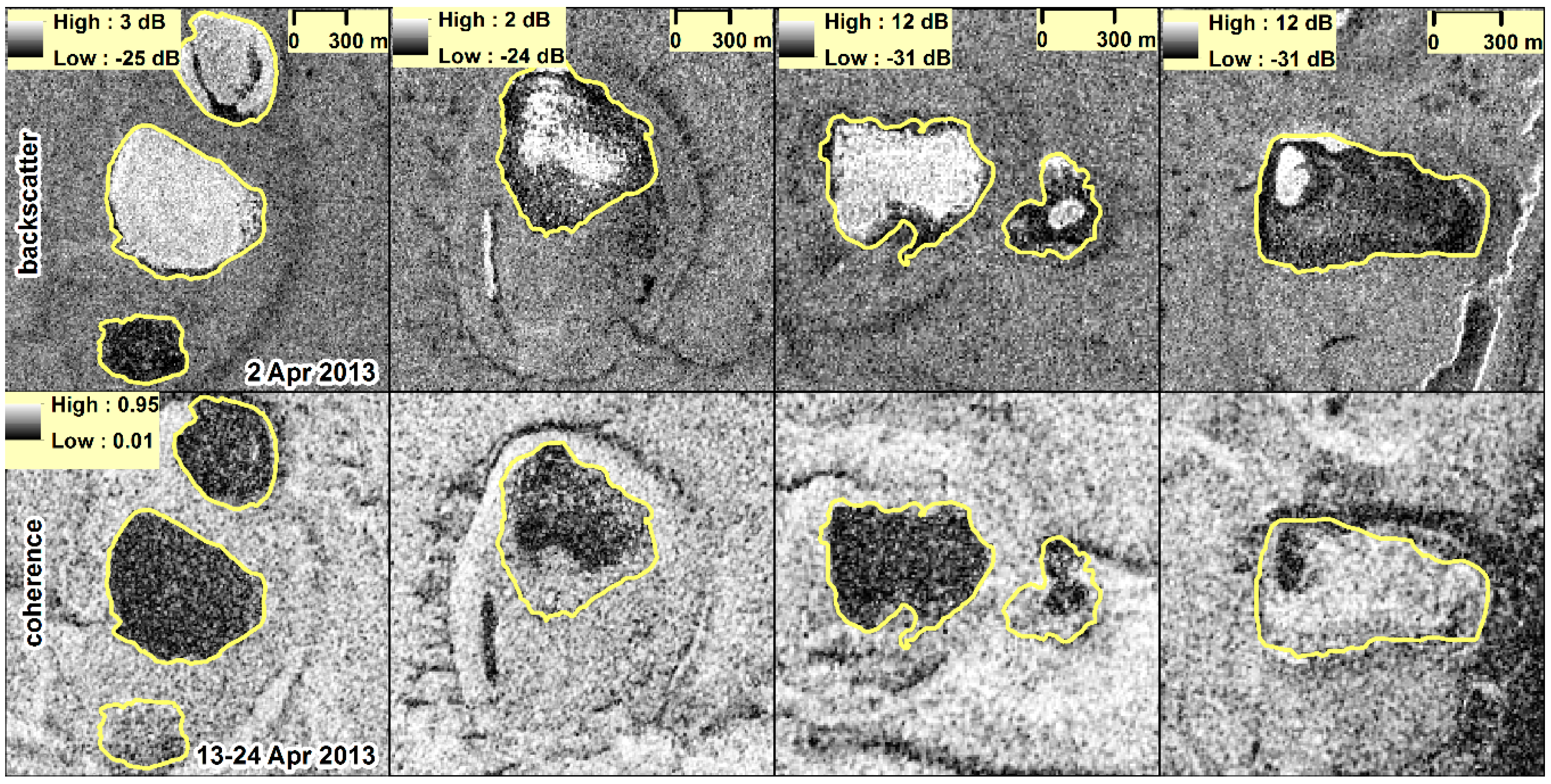
5.1. Ice Grounding
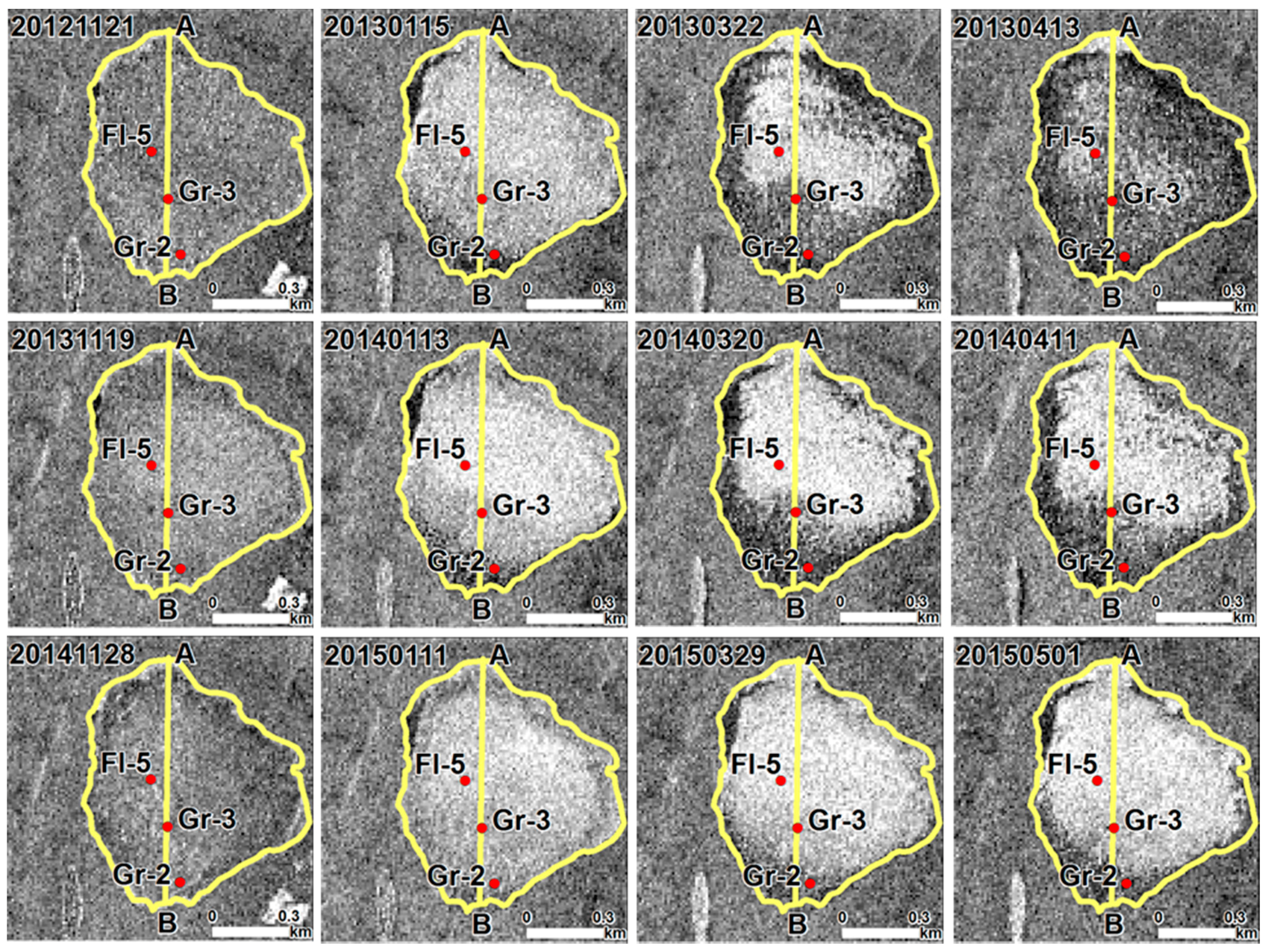
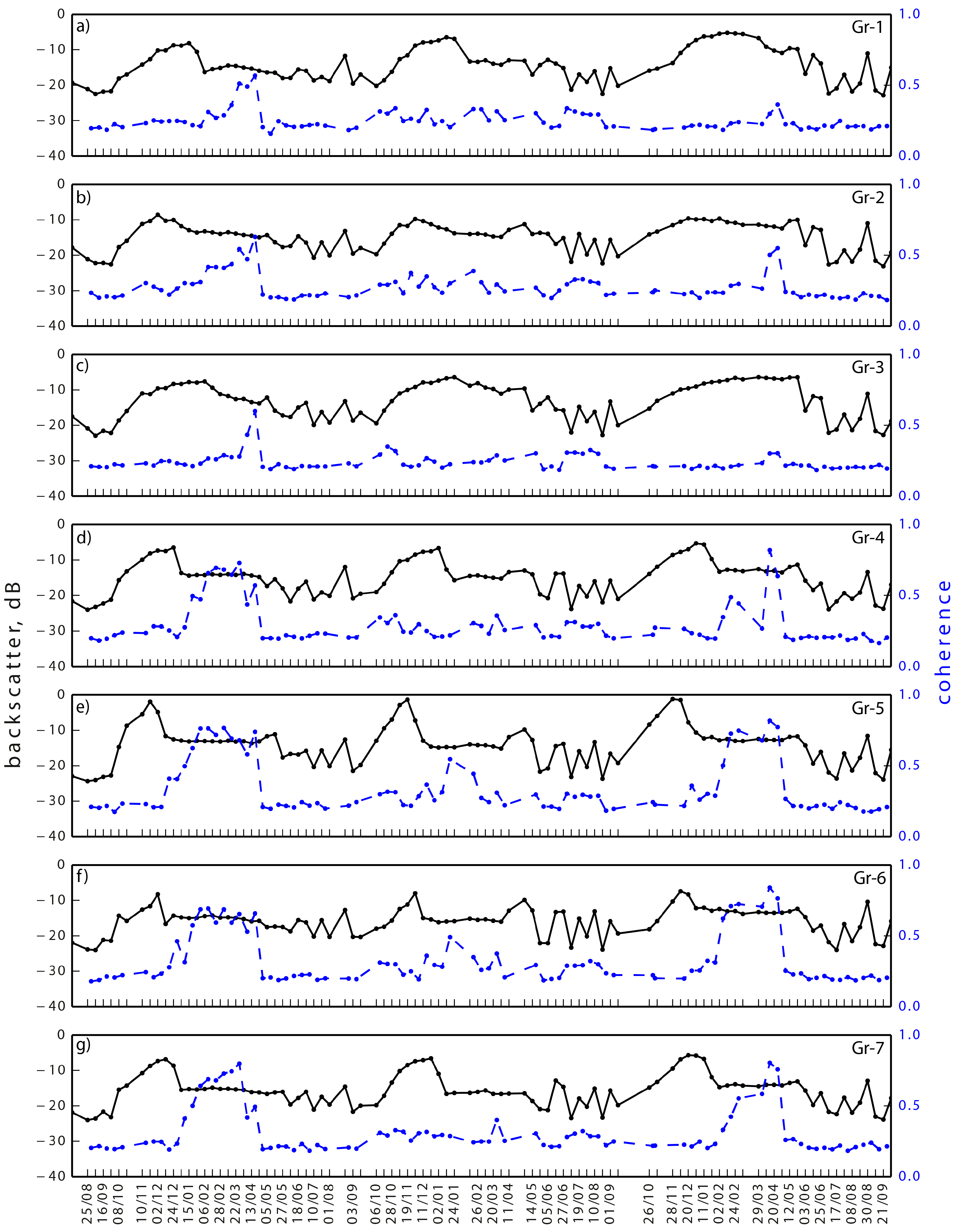
5.1.1. Backscatter Intensity Time Series
5.1.2. SAR- and CLIMo-Derived Ice Thicknesses Versus in Situ Measured Ice Thicknesses
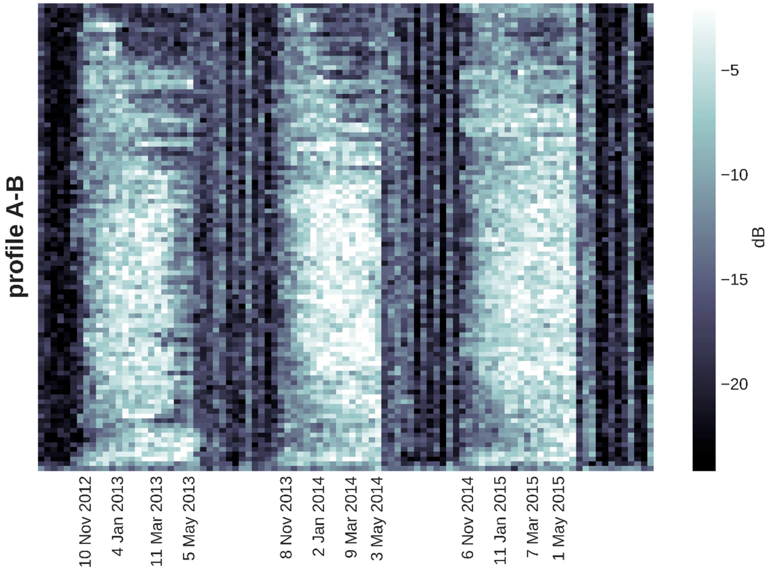
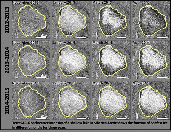
5.1.3. Spatio-Temporal Variability of Bedfast Ice
5.1.4. Coherence Time Series
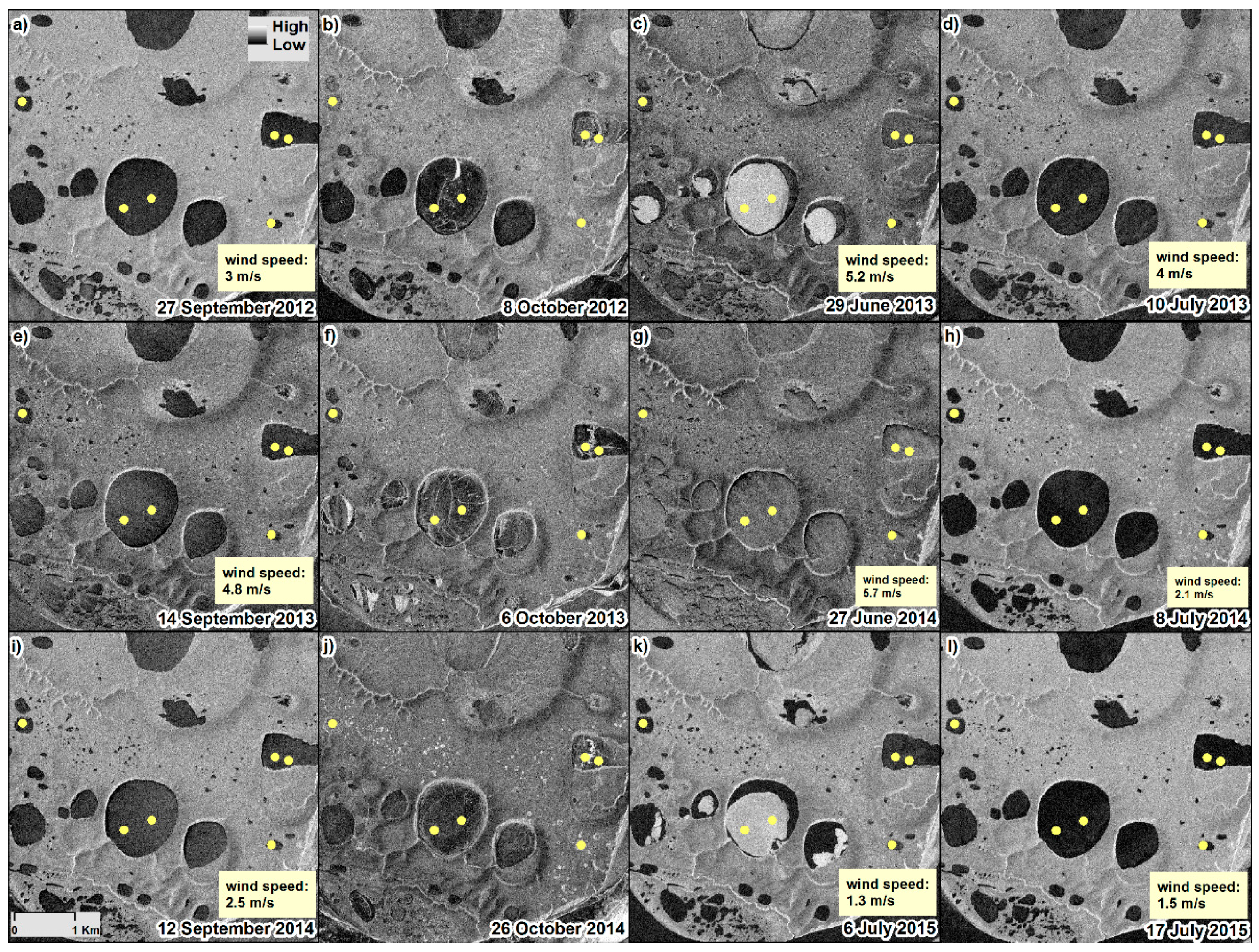
5.2. Ice Phenology
5.2.1. Freeze Up and Ice Growth
5.2.2. Melt Onset
5.2.3. Water-Clear-of-Ice
6. Discussion
6.1. Ice Grounding
6.1.1. Backscatter Intensity
6.1.2. Model Results
6.1.3. Spatio-Temporal Variability of Bedfast Ice
6.1.4. Coherence
6.2. Ice Phenology
6.2.1. Freeze Onset
6.2.2. Melt Onset
6.2.3. Water-Clear-of-Ice
7. Conclusions
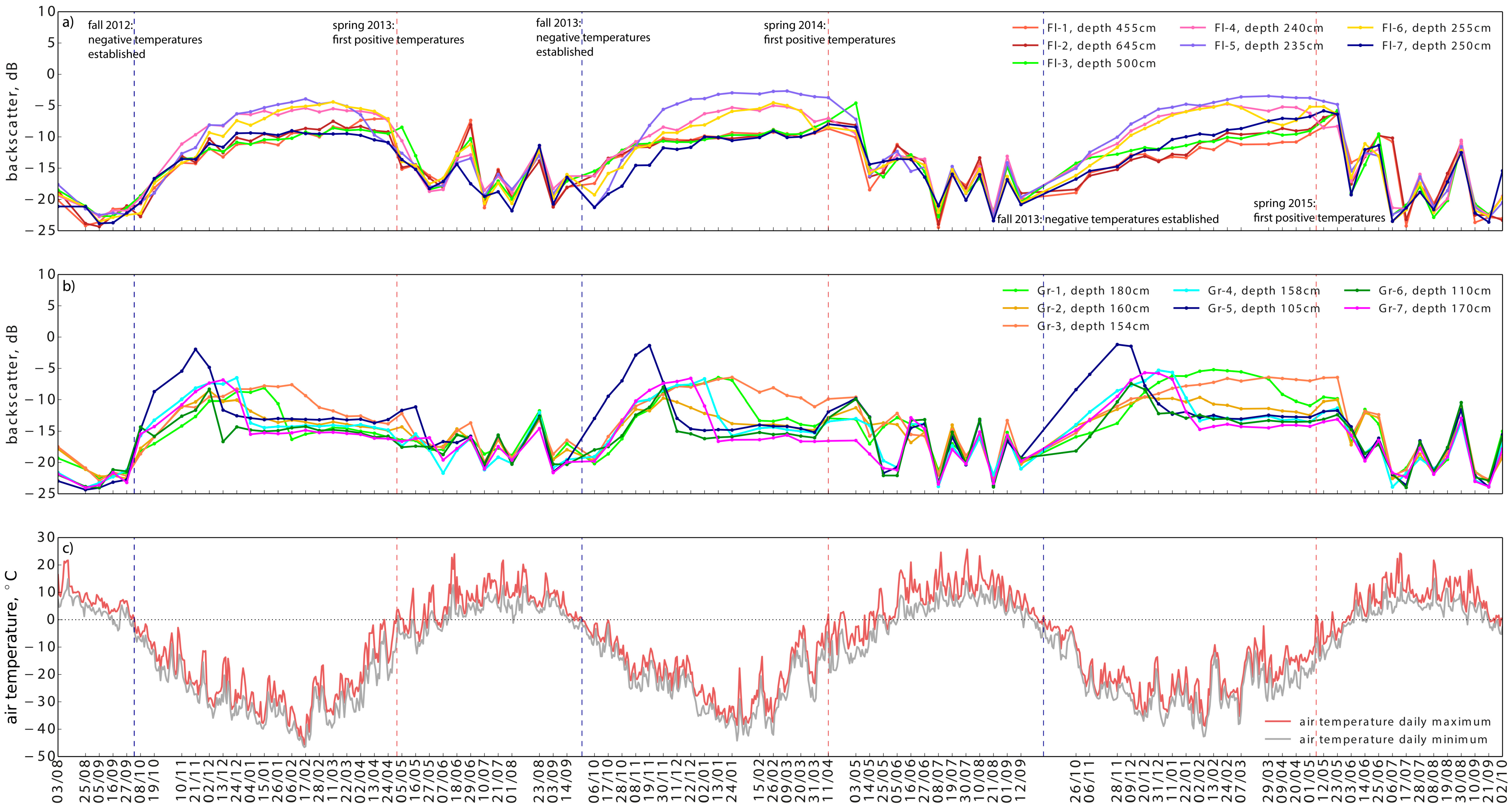
- Ice phenology stages, such as (i) the onset of freezing as well as ice thickening; (ii) the onset of surface melt; and (iii) the date of complete ice-off condition were generally tracked by TSX backscatter intensity time series. Dates of ice-on and ice-off were in range of those simulated by CLIMo. The onset of the surface melt was marked by a strong drop in coherence, which was more time-consistent for different locations than changes in backscatter intensity.
- Lake ice grounding was well detected by a prominent drop in TSX backscatter intensity in winter. Most of the field measurements confirmed the TSX-derived separation between floating and bedfast ice. An increase in interferometric coherence was observed for grounded ice for two of the three ice seasons, confirming the detection of bedfast ice. The gradual increase of coherence occurred typically later than the backscatter drop, probably reflecting the freezing of lake sediments.
- The high temporal resolution of the TSX time series (compared to previous satellite-based SAR studies) generally improved the extraction of the timing of ice grounding. However, we encountered some difficulties in the timing extraction, which are likely related to (i) a mixed signal from both floating and grounded ice within the ROI and (ii) propagation of the freezing front into lake sediments which affects SAR signal return.
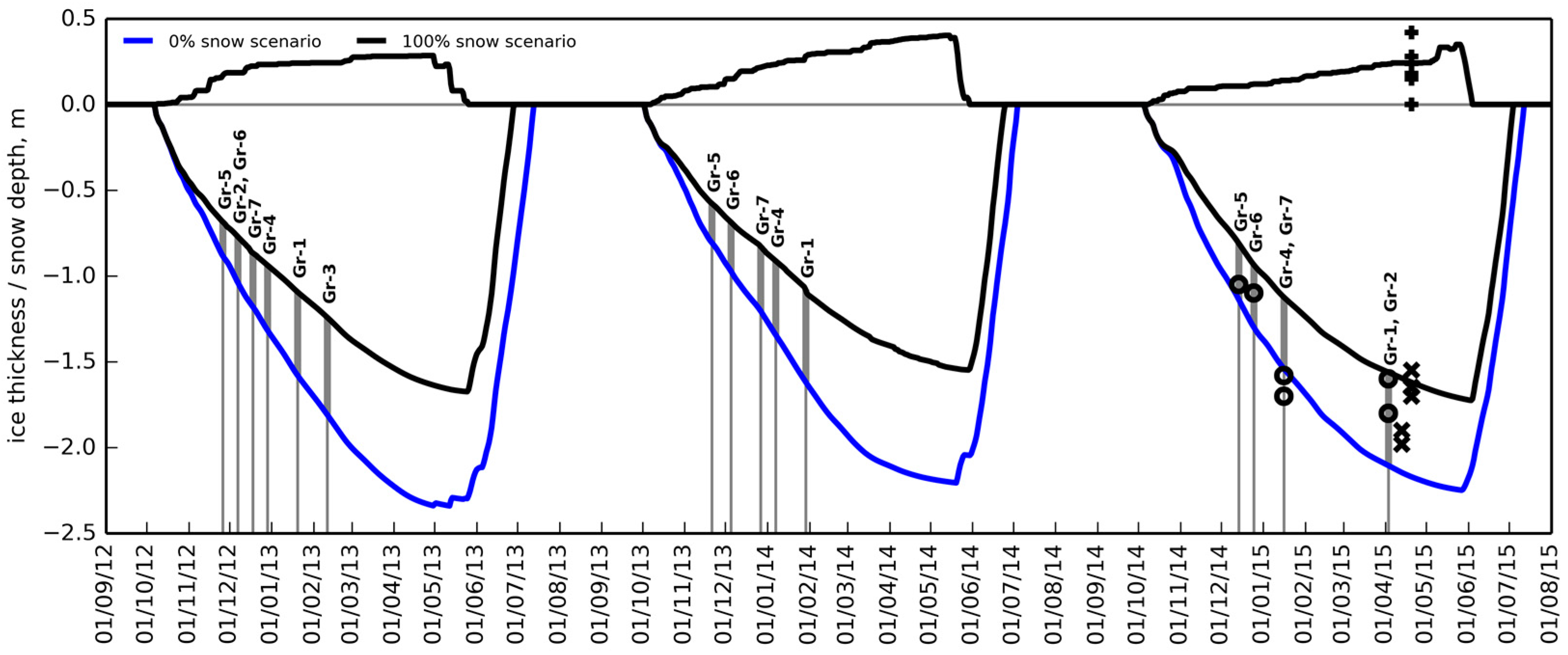
- Using the timing of ice grounding and simulated ice thickness we obtained the water depth at grounded ice locations where in situ ice thicknesses were available. Comparison showed a reasonably good agreement in the year of field measurements and a larger difference in the previous two years.
- Both ice phenology and ice grounding revealed interannual variability, most likely due to a difference in climatic conditions and water levels between the years.
- The high spatial and temporal resolution of TSX imagery allows monitoring the progression of the ice grounding for an entire lake which could be used for lake bathymetry extraction in future. Furthermore, the high coherence observed over the shallow lakes indicates that the bathymetry of these lakes could be derived with SAR interferometry in future studies.
Supplementary Materials
Acknowledgments
Author Contributions
Conflicts of Interest
References
- Lafleur, P.M.; Wurtele, A.B.; Duguay, C.R. Spatial and temporal variations in surface albedo of a subarctic landscape using surface-based measurements and remote sensing. Arct. Alp. Res. 1997, 29, 261–269. [Google Scholar] [CrossRef]
- Pienitz, R.; Doran, P.T.; Lamoureux, S.F. Origin and geomorphology of lakes in the polar regions. In Polar Lakes and Rivers: Limnology of Arctic and Antarctic Aquatic Ecosystems; Warwick, F.V., Laybourn-Parry, J., Eds.; Oxford University Press: Oxford, UK, 2008; pp. 25–41. [Google Scholar]
- Grosse, G.; Jones, B.; Arp, C. Thermokarst lakes, drainage, and drained basins. In Treatise on Geomorphology; Shroder, J.F., Giardino, R., Harbor, J., Eds.; Academic Press: San Diego, CA, USA, 2013; Volume 8, pp. 325–353. [Google Scholar]
- Zimov, S.A.; Voropaev, Y.V.; Semiletov, I.P.; Davidov, S.P.; Prosiannikov, S.F.; Chapin, F.S., III; Trumbore, S.; Tyler, S. North Siberian lakes: A methane source fueled by Pleistocene carbon. Science 1997, 277, 800–802. [Google Scholar] [CrossRef]
- Rouse, W.R.; Oswald, C.J.; Binyamin, J.; Spence, C.; Schertzer, W.M.; Blanken, P.D.; Bussières, N.; Duguay, C.R. Role of northern lakes in a regional energy balance. J. Hydrometeorol. 2005, 6, 291–305. [Google Scholar] [CrossRef]
- Brown, L.C.; Duguay, C.R. The response and role of ice cover in lake-climate interactions. Prog. Phys. Geogr. 2010, 34, 671–704. [Google Scholar] [CrossRef]
- Langer, M.; Westermann, S.; Muster, S.; Piel, K.; Boike, J. The surface energy balance of a polygonal tundra site in northern Siberia Part 2: Winter. Cryosphere 2011, 5, 509–524. [Google Scholar] [CrossRef] [Green Version]
- Lenormand, F.; Duguay, C.R.; Gauthier, R. Development of a historical database for the study of climate change in Canada. Hydrol. Process. 2002, 16, 3707–3722. [Google Scholar] [CrossRef]
- Duguay, C.R.; Prowse, T.D.; Bonsal, B.R.; Brown, R.D.; Lacroix, M.P.; Ménard, P. Recent trends in Canadian lake ice cover. Hydrol. Process. 2006, 20, 781–801. [Google Scholar] [CrossRef]
- Jeffries, M.O.; Zhang, T.; Frey, K.; Kozlenko, N. Estimating late-winter heat flow to the atmosphere from the lake dominated Alaskan North Slope. J. Glaciol. 1999, 45, 315–324. [Google Scholar] [CrossRef]
- Langer, M.; Westermann, S.; Walter Anthony, K.; Wischnewski, K.; Boike, J. Frozen ponds: Production and storage of methane during the Arctic winter in a lowland tundra landscape in northern Siberia, Lena River delta. Biogeosciences 2015, 12, 977–990. [Google Scholar] [CrossRef]
- Arp, C.D.; Jones, B.M.; Lu, Z.; Whitman, M.S. Shifting balance of thermokarst lake ice regimes across the Arctic Coastal Plain of northern Alaska. Geophys. Res. Lett. 2012, 39, L16503. [Google Scholar] [CrossRef]
- Surdu, C.M.; Duguay, C.R.; Brown, L.C.; Fernández Prieto, D. Response of ice cover on shallow lakes of the North Slope of Alaska to contemporary climate conditions (1950–2011): Radar remote-sensing and numerical modeling data analysis. Cryosphere 2014, 8, 167–180. [Google Scholar] [CrossRef] [Green Version]
- Arp, C.D.; Jones, B.M.; Urban, F.E.; Grosse, G. Hydrogeomorphic processes of thermokarst lakes with grounded-ice and floating-ice regimes on the Arctic coastal plain, Alaska. Hydrol. Process. 2011, 25, 2422–2438. [Google Scholar] [CrossRef]
- Latifovic, R.; Pouliot, D. Analysis of climate change impacts on lake ice phenology in Canada using the historical satellite data record. Remote Sens. Environ. 2007, 106, 492–507. [Google Scholar] [CrossRef]
- Weber, H.; Riffler, M.; Nõges, T.; Wunderle, S. Lake ice phenology from AVHRR data for European lakes: An automated two-step extraction method. Remote Sens. Environ. 2016, 174, 329–340. [Google Scholar] [CrossRef]
- Hall, D.K.; Fagre, D.B.; Klasner, F.; Linebaugh, G.; Liston, G.E. Analysis of ERS-1 synthetic aperture radar data of frozen lakes in northern Montana and implications for climate studies. J. Geophys. Res. Oceans 1994, 22473–22482. [Google Scholar] [CrossRef]
- Howell, S.E.L.; Brown, L.C.; Kang, K.-K.; Duguay, C.R. Variability in ice phenology on Great Bear Lake and Great Slave Lake, Northwest Territories, Canada, from SeaWinds/QuikSCAT: 2000–2006. Remote Sens. Environ. 2009, 113, 816–834. [Google Scholar] [CrossRef]
- Cook, T.L.; Bradley, R.S. An analysis of past and future changes in the ice cover of two High-Arctic lakes based on synthetic aperture radar (SAR) and Landsat imagery. Arct. Antarct. Alp. Res. 2010, 42, 9–18. [Google Scholar] [CrossRef]
- Surdu, C.M.; Duguay, C.R.; Kheyrollah Pour, H.; Brown, L.C. Ice freeze-up and break-up detection of shallow lakes in Northern Alaska with spaceborne SAR. Remote Sens. 2015, 7, 6133–6159. [Google Scholar] [CrossRef]
- Elachi, C.; Bryan, M.L.; Weeks, W.F. Imaging radar observations of frozen Arctic lakes. Remote Sens. Environ. 1976, 5, 169–175. [Google Scholar] [CrossRef]
- Weeks, W.F.; Sellmann, P.; Campbell, W.J. Interesting features of radar imagery of ice-covered North Slope lakes. J. Glaciol. 1977, 18, 129–136. [Google Scholar]
- Weeks, W.F.; Fountain, A.G.; Bryan, M.L.; Elachi, C. Differences in radar return from ice-covered North Slope Lakes. J. Geophys. Res. Oceans 1978, 83, 4069–4073. [Google Scholar] [CrossRef]
- Jeffries, M.O.; Morris, K.; Weeks, W.F.; Wakabayashi, H. Structural-stratigraphic features and ERS-1 SAR backscatter characteristics of ice growing on shallow lakes in NW Alaska, winter 1991–92. J. Geophys. Res. Oceans 1994, 99, 22459–22471. [Google Scholar] [CrossRef]
- Morris, K.; Jeffries, M.O.; Weeks, W.F. Ice processes and growth history on Arctic and sub-Arctic lakes using ERS-1 SAR data. Polar Rec. 1995, 31, 115–128. [Google Scholar] [CrossRef]
- Jeffries, M.O.; Morris, K.; Liston, G.E. A method to determine lake depth and water availability on the North Slope of Alaska with spaceborne imaging radar and numerical ice growth modelling. Arctic 1996, 49, 367–374. [Google Scholar] [CrossRef]
- Duguay, C.R.; Pultz, T.J.; Lafleur, P.M.; Drai, D. RADARSAT backscatter characteristics of ice growing on shallow sub-Arctic lakes, Churchill, Manitoba, Canada. Hydrol. Process. 2002, 16, 1631–1644. [Google Scholar] [CrossRef]
- Duguay, C.R.; Lafleur, P.M. Determining depth and ice thickness of shallow sub-Arctic lakes using space-borne optical and SAR data. Int. J. Remote Sens. 2003, 24, 475–489. [Google Scholar] [CrossRef]
- Hirose, T.; Kapfer, M.; Bennett, J.; Cott, P.; Manson, G.; Solomon, S. Bottomfast ice mapping and the measurement of ice thickness on tundra lakes using C-Band Synthetic Aperture Radar remote sensing. J. Am. Water Resour. Assoc. 2008, 44, 285–292. [Google Scholar] [CrossRef]
- Jones, B.M.; Gusmeroli, A.; Arp, C.D.; Strozzi, T.; Grosse, G.; Gaglioti, B.V.; Whitman, M.S. Classification of freshwater ice conditions on the Alaskan Arctic Coastal Plain using ground penetrating radar and TerraSAR-X satellite data. Int. J. Remote Sens. 2013, 34, 8253–8265. [Google Scholar] [CrossRef]
- Sobiech, J.; Dierking, W. Observing lake- and river-ice decay with SAR: advantages and limitations of the unsupervised k-means classification approach. Ann. Glaciol. 2013, 54, 65–72. [Google Scholar] [CrossRef]
- Kozlenko, N.; Jeffries, M.O. Bathymetric mapping of shallow water in thaw lakes on the North Slope of Alaska with spaceborne imaging radar. Arctic 2000, 53, 306–316. [Google Scholar] [CrossRef]
- Gunn, G.E.; Duguay, C.R.; Brown, L.C.; King, J.; Atwood, D.; Kasurak, A. Freshwater lake ice thickness derived using X- and Ku-band FMCW scatterometers. Cold Reg. Sci. Technol. 2015, 120, 115–126. [Google Scholar] [CrossRef]
- Kaatze, U.; Uhlendorf, V. The dielectric properties of water at microwave frequencies. Zeitschrift für Physikalische Chemie 1981, 126, 151–165. [Google Scholar] [CrossRef]
- Vant, M.R.; Gray, R.B.; Ramseier, R.O.; Makios, V. Dielectric properties of fresh and sea ice at 10 and 35 GHz. J. Appl. Phys. 1974, 45, 4712–4717. [Google Scholar] [CrossRef]
- Engram, M.; Walter Anthony, K.M.; Meyer, F.J.; Grosse, G. Characterization of L-band synthetic aperture radar (SAR) backscatter from floating and grounded thermokarst lake ice in Arctic Alaska. Cryosphere 2013, 7, 1741–1752. [Google Scholar] [CrossRef]
- Atwood, D.K.; Gunn, G.E.; Roussi, C.; Wu, J.; Duguay, C.; Sarabandi, K. Microwave backscatter from Arctic lake ice and polarimetric implications. IEEE Trans. Geosci. Remote Sens. 2015, 53, 5972–5982. [Google Scholar] [CrossRef]
- Hoekstra, P.; Delaney, A. Dielectric properties of soils at UHF and microwave frequencies. J. Geophys. Res. 1974, 79, 1699–1708. [Google Scholar] [CrossRef]
- Brown, R.S.; Duguay, C.R.; Mueller, R.P.; Moulton, L.L.; Doucette, P.J.; Tagestad, J.D. Use of Synthetic Aperture Radar (SAR) to identify and characterize overwintering areas of fish in ice-covered arctic rivers: A demonstration with Broad Whitefish and their habitats in the Sagavanirktok River, Alaska. Trans. Am. Fish. Soc. 2010, 139, 1711–1722. [Google Scholar] [CrossRef]
- Gunn, G.E.; Brogioni, M.; Duguay, C.; Macelloni, G.; Kasurak, A.; King, J. Observation and modeling of X-and Ku-band backscatter of snow-covered freshwater lake ice. IEEE J. Sel. Top. Appl. Earth Obs. Remote Sens. 2015, 8, 3629–3642. [Google Scholar] [CrossRef]
- Zebker, H.A.; Villasenor, J. Decorrelation in interferometric radar echoes. IEEE Trans. Geosci. Remote Sens. 1992, 30, 950–959. [Google Scholar] [CrossRef]
- Geldsetzer, T.; van der Sanden, J.; Brisco, B. Monitoring lake ice during spring melt using RADARSAT-2 SAR. Can. J. Remote Sens. 2010, 36, S391–S400. [Google Scholar] [CrossRef]
- Grigoriev, N.F. The temperature of permafrost in the Lena Delta basin: Deposit conditions and properties of the permafrost in Yakutia (in Russian). Yakutsk 1960, 2, 97–101. [Google Scholar]
- Muster, S.; Langer, M.; Heim, B.; Westermann, S.; Boike, J. Subpixel heterogeneity of ice-wedge polygonal tundra: a multi-scale analysis of land cover and evapotranspiration in the Lena River Delta, Siberia. Tellus B 2012, 64, 17301. [Google Scholar] [CrossRef]
- Boike, J.; Kattenstroth, B.; Abramova, K.; Bornemann, N.; Chetverova, A.; Fedorova, I.; Fröb, K.; Grigoriev, M.; Grüber, M.; Kutzbach, L.; et al. Baseline characteristics of climate, permafrost and land cover from a new permafrost observatory in the Lena River Delta, Siberia (1998–2011). Biogeosciences 2013, 10, 2105–2128. [Google Scholar] [CrossRef] [Green Version]
- Morgenstern, A.; Grosse, G.; Günther, F.; Fedorova, I.; Schirrmeister, L. Spatial analyses of thermokarst lakes and basins in Yedoma landscapes of the Lena Delta. Cryosphere 2011, 5, 849–867. [Google Scholar] [CrossRef] [Green Version]
- Werner, C.; Wegmüller, U.; Strozzi, T.; Wiesmann, A. Gamma SAR and interferometric processing software. In Proceedings of the ERS-Envisat Symposium, Gothenburg, Sweden, 16–20 October 2000.
- Duguay, C.R.; Flato, G.M.; Jeffries, M.O.; Ménard, P.; Morris, K.; Rouse, W.R. Ice-cover variability on shallow lakes at high latitudes: model simulations and observations. Hydrol. Process. 2003, 17, 3465–3483. [Google Scholar] [CrossRef]
- Jeffries, M.O.; Morris, K.; Duguay, C.R. Lake ice growth and decay in central Alaska, USA: Observations and computer simulations compared. Ann. Glaciol. 2005, 40, 195–199. [Google Scholar] [CrossRef]
- Brown, L.C.; Duguay, C.R. A comparison of simulated and measured lake ice thickness using a Shallow Water Ice Profiler. Hydrol. Process. 2011, 25, 2932–2941. [Google Scholar] [CrossRef]
- Reliable Prognosis RP5. Available online: http://rp5.ru/Weather_archive_on_Stolb_Island (accessed on 18 October 2016).
- Sturm, M.; Liston, G.E. The snow cover on lakes of the Arctic Coastal Plain of Alaska, USA. J. Glaciol. 2003, 49, 370–380. [Google Scholar] [CrossRef]
- Rott, H.; Nagler, T.; Scheiber, R. Snow mass retrieval by means of SAR interferometry. In Proceedings of the FRINGE Workshop (ESA SP-550), Frascati, Italy, 1–5 December 2003.
- Strozzi, T.; Wiesmann, A.; Mätzler, C. Active microwave signatures of snow covers at 5.3 and 35 GHz. Radio Sci. 1997, 32, 479–495. [Google Scholar] [CrossRef]
- Strozzi, T.; Wegmuller, U.; Matzler, C. Mapping wet snowcovers with SAR interferometry. Int. J. Remote Sens. 1999, 20, 2395–2403. [Google Scholar] [CrossRef]
- Antonova, S.; Kääb, A.; Heim, B.; Langer, M.; Boike, J. Spatio-temporal variability of X-band radar backscatter and coherence over the Lena River Delta, Siberia. Remote Sens. Environ. 2016, 182, 169–191. [Google Scholar] [CrossRef]
- Arp, C.D.; Jones, B.M.; Liljedahl, A.K.; Hinkel, K.M.; Welker, J.A. Depth, ice thickness, and ice-out timing cause divergent hydrologic responses among Arctic lakes. Water Resour. Res. 2015, 51, 9379–9401. [Google Scholar] [CrossRef]


| Reference | Study Area | Sensor | Polarization | Incidence Angle | Magnitude of Drop in Backscatter from Floating to Grounded Ice (in dB) |
|---|---|---|---|---|---|
| Jeffries et al. [24] | Alaska North Slope | ERS-1 (C-band) | VV | 20.1–25.9° | 10–12 |
| Morris et al. [25] | Alaska North Slope, Yukon Delta, Bristol Bay | ERS-1 (C-band) | VV | 20.1–25.9° | 4.8–8.8 (sub-Arctic lakes) |
| 7.8–11.8 (Arctic lakes) | |||||
| Duguay et al. [27] | Churchill, Manitoba | RADARSAT-1 (C-band) | HH | 20–49° | 6 |
| Brown et al. [39] | Sagavanirktok River delta, Alaska | ASAR AP (C-band) | HH, VV | 19.2–31.4° | threshold: −10 * |
| HV, VH | threshold: −19 | ||||
| Engram et al. [36] | northern Seward Peninsula, Arctic Coastal Plain | ALOS PALSAR, JERS-1 (L-band) | HH | 24–40° | 3–6 |
| ERS-1,-2 (C-band) | VV | 23° | 8–9 | ||
| Jones et al. [30] | Arctic Coastal Plain | TSX (X-band) | HH | 46° | threshold: −12.3 |
| Gunn et al. [40] | Churchill, Manitoba | Field-based scatterometer (X- & Ku-band) | VV, VH | 39–45° | 2–4 |
| No. | Date | Name | Lon, E | Lat, N | Snow Cover, m | Ice Thickness, m | Total Depth, m |
|---|---|---|---|---|---|---|---|
| 1 | 13 April 2015 | Fl-1 | 126.1785 | 72.2987 | 0 | 1.90 | 4.55 |
| 2 | 13 April 2015 | Fl-2 | 126.1653 | 72.2971 | 0 | 1.98 | 6.45 |
| 3 | 20 April 2015 | Fl-3 | 126.1507 | 72.4592 | 0.28 | 1.55 | 5.00 |
| 4 | 20 April 2015 | Fl-4 | 126.1433 | 72.4522 | 0.15 | 1.65 | 2.40 |
| 5 | 20 April 2015 | Gr-1 | 126.1390 | 72.4449 | 0.15 | 1.80 | 1.80 |
| 6 | 20 April 2015 | Fl-5 | 126.1052 | 72.4220 | 0.15 | 1.65 | 2.35 |
| 7 | 20 April 2015 | Gr-2 | 126.1092 | 72.4184 | 0.18 | 1.60 | 1.60 |
| 8 | 20 April 2015 | Gr-3 | 126.1074 | 72.4203 | 0 | 1.54 | 1.54 |
| 9 | 20 April 2015 | Fl-6 | 126.1389 | 72.3952 | 0.24 | 1.65 | 2.55 |
| 10 | 20 April 2015 | Fl-7 | 126.1586 | 72.3940 | 0.42 | 1.70 | 2.50 |
| 11 | 20 April 2015 | Gr-4 | 126.1134 | 72.3121 | 0 | 1.58 | 1.58 |
| 12 | 20 April 2015 | Gr-5 | 126.2370 | 72.3088 | 0 | 1.05 | 1.05 |
| 13 | 20 April 2015 | Gr-6 | 126.2436 | 72.3084 | 0 | 1.10 | 1.10 |
| 14 | 13 April 2015 | Gr-7 | 126.2371 | 72.2959 | 0 | 1.70 | 1.70 |
| Location | 2012–2013 | 2013–2014 | 2014–2015 | |||
|---|---|---|---|---|---|---|
| Date of the First Backscatter Drop | Magnitude of the Drop, dB | Date of the First Backscatter Drop | Magnitude of the Drop, dB | Date of the First Backscatter Drop | Magnitude of the Drop, dB | |
| Gr-1, 180 cm | 26 January | 2.5 | 15 February * | 6.4 | 9 April | 2.5 |
| Gr-7, 170 cm | 24 December | 1.8 | 2 January | 4.4 | 22 January | 5.2 |
| Gr-2, 160 cm | 13 December | 1.7 | no clear drop | no clear drop | ||
| Gr-4, 158 cm | 4 January | 7.2 | 13 January | 6 | 22 January | 4.1 |
| Gr-3, 154 cm | 17 February | 1.8 | 15 February * | 2.4 | no drop | |
| Gr-6, 110 cm | 13 December | 8.3 | 11 December | 7 | 31 December | 3.8 |
| Gr-5, 105 cm | 2 December | 2.9 | 30 November | 5.9 | 20 December | 6.3 |
| Location | In Situ Measured Ice Thickness, m (April, 2015) | Simulated Ice Thickness by the Time of Ice Grounding, m (100% to 0% snow cover scenario) | ||
|---|---|---|---|---|
| 2012–2013 | 2013–2014 | 2014–2015 | ||
| Gr-5 | 1.05 | 0.68–0.88 | 0.58–0.81 | 0.81–1.14 |
| Gr-6 | 1.1 | 0.77–1.04 | 0.69–0.97 | 0.93–1.3 |
| Gr-3 | 1.54 | 1.24–1.81 | ||
| Gr-4 | 1.58 | 0.94–1.32 | 0.91–1.34 | 1.12–1.54 |
| Gr-2 | 1.6 | 0.77–1.04 | 1.56–2.1 | |
| Gr-7 | 1.7 | 0.86–1.18 | 0.83–1.2 | 1.12–1.54 |
| Gr-1 | 1.8 | 1.09–1.58 | 1.08–1.62 | 1.56–2.1 |
| Location | 2012–2013 | 2013–2014 | 2014–2015 | |||
|---|---|---|---|---|---|---|
| Period of the First Coherence Increase | Coherence | Period of the First Coherence Increase | Coherence | Period of the First Coherence Increase | Coherence | |
| Gr-1, 180 cm | 6–17 February | 0.3 | - | - | 20 April–1 May | 0.36 |
| Gr-7, 170 cm | 4–15 January | 0.41 | 20–31 March | 0.4 | 13–24 February | 0.42 |
| Gr-2, 160 cm | 6–17 February | 0.42 | - | - | 9–20 April | 0.5 |
| Gr-4, 158 cm | 15–26 January | 0.5 | - | - | 13–24 February | 0.49 |
| Gr-3, 154 cm | 2–13 April | 0.43 | - | - | - | - |
| Gr-6, 110 cm | 24 December–4 January | 0.46 | 13–24 January | 0.5 | 2–13 February | 0.62 |
| Gr-5, 105 cm | 13–24 December | 0.4 | 13–24 January | 0.55 | 2–13 February | 0.5 |
| Location | Depth, m | Ice Thickness, m | Mean Backscatter in 2012–2013 (24 December–2 April), dB | Mean Backscatter in 2013–2014 (30 November–11 April), dB | Mean Backscatter in 2014–2015 (31 December–1 May), dB |
|---|---|---|---|---|---|
| Fl-1 | 4.55 | 1.9 | −9.8 ± 1.3 | −9.7 ± 0.5 | −11.7 ± 1.2 |
| Fl-2 | 6.45 | 1.98 | −9.2 ± 1 | −9.7 ± 1 | −10.5 ± 1.8 |
| Fl-3 | 5.0 | 1.55 | −9.9 ± 0.9 | −9.7 ± 1 | −10.4 ± 1 |
| Fl-4 | 2.4 | 1.65 | −6 ± 0.4 | −6.6 ± 1.3 | −5.6 ± 0.6 |
| Fl-5 | 2.35 | 1.65 | −5.2 ± 0.8 | −3.6 ± 0.8 | −4.3 ± 0.7 |
| Fl-6 | 2.55 | 1.65 | −5.9 ± 1.2 | −7.2 ± 1.7 | −6.3 ± 1.2 |
| Fl-7 | 2.5 | 1.7 | −9.5 ± 0.2 | −10.2 ± 1.1 | −8.9 ± 1.6 |
| Ice-on TSX (Deep and Shallow) | Ice-on CLIMo (Deep) | Ice-on CLIMo (Shallow) | Ice-off TSX | Ice-off CLIMo | |
|---|---|---|---|---|---|
| 2012–2013 | Between 27 September and 8 October | 7 October | 3 October | Latest by 10 July (29 June shows significant ice coverage) | 30 June–15 July (depending on snow cover scenario) |
| 2013–2014 | Between 14 September and 6 October (one missing image in between) | 4 October | 27 September | By 27 June (based on comparison with previous year because image is affected by wind) | 26 June–6 July (depending on snow cover scenario) |
| 2014–2015 | Three missing images | 7 October | 27 September | Latest by 17 July (6 July shows significant ice coverage for some big lakes) | 6 July–14 July (depending on snow cover scenario) |
© 2016 by the authors; licensee MDPI, Basel, Switzerland. This article is an open access article distributed under the terms and conditions of the Creative Commons Attribution (CC-BY) license (http://creativecommons.org/licenses/by/4.0/).
Share and Cite
Antonova, S.; Duguay, C.R.; Kääb, A.; Heim, B.; Langer, M.; Westermann, S.; Boike, J. Monitoring Bedfast Ice and Ice Phenology in Lakes of the Lena River Delta Using TerraSAR-X Backscatter and Coherence Time Series. Remote Sens. 2016, 8, 903. https://doi.org/10.3390/rs8110903
Antonova S, Duguay CR, Kääb A, Heim B, Langer M, Westermann S, Boike J. Monitoring Bedfast Ice and Ice Phenology in Lakes of the Lena River Delta Using TerraSAR-X Backscatter and Coherence Time Series. Remote Sensing. 2016; 8(11):903. https://doi.org/10.3390/rs8110903
Chicago/Turabian StyleAntonova, Sofia, Claude R. Duguay, Andreas Kääb, Birgit Heim, Moritz Langer, Sebastian Westermann, and Julia Boike. 2016. "Monitoring Bedfast Ice and Ice Phenology in Lakes of the Lena River Delta Using TerraSAR-X Backscatter and Coherence Time Series" Remote Sensing 8, no. 11: 903. https://doi.org/10.3390/rs8110903