
Long-Term Post-Disturbance Forest Recovery in the Greater Yellowstone Ecosystem Analyzed Using Landsat Time Series Stack

 ,
, 
 and
and 
Abstract
:
1. Introduction
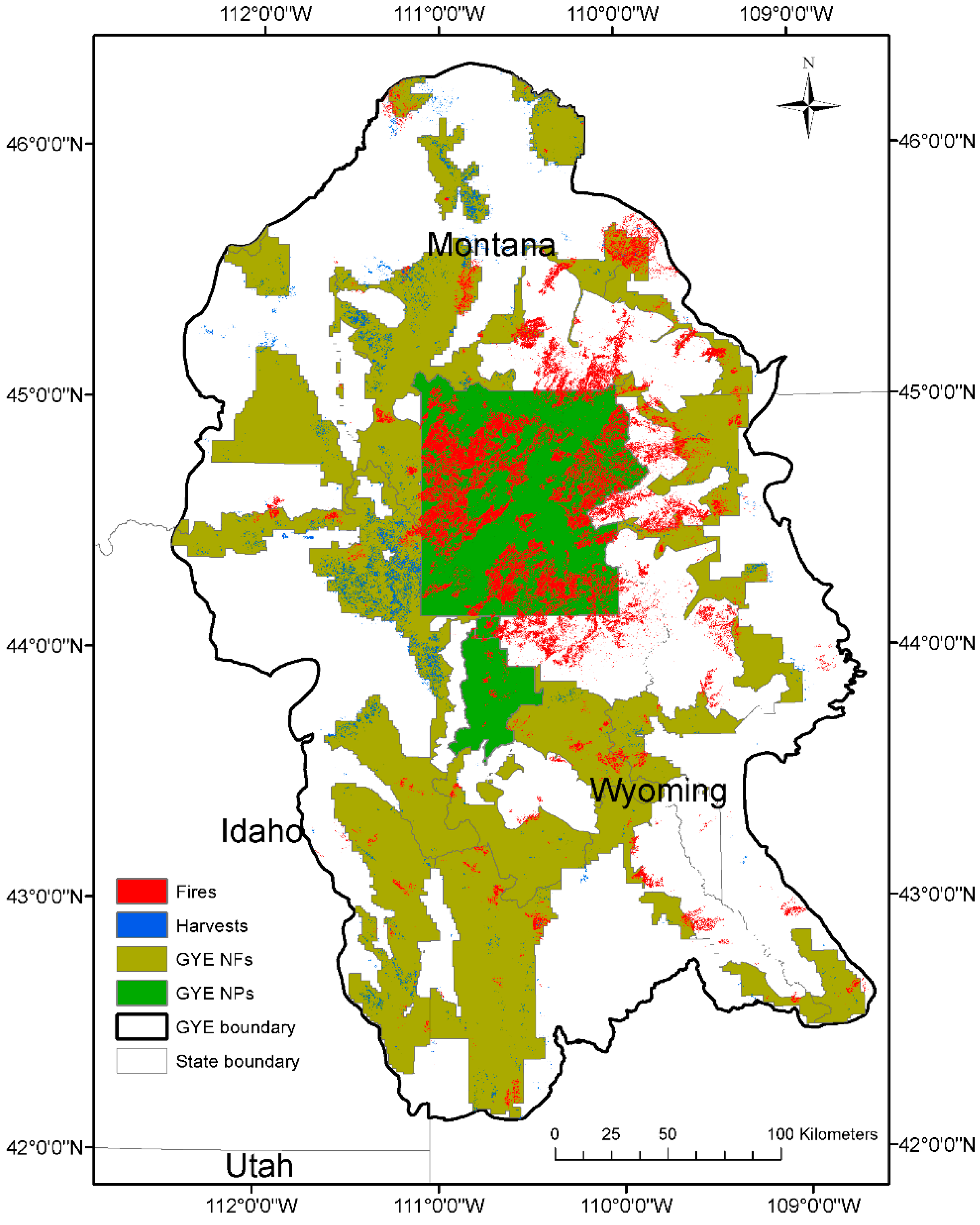
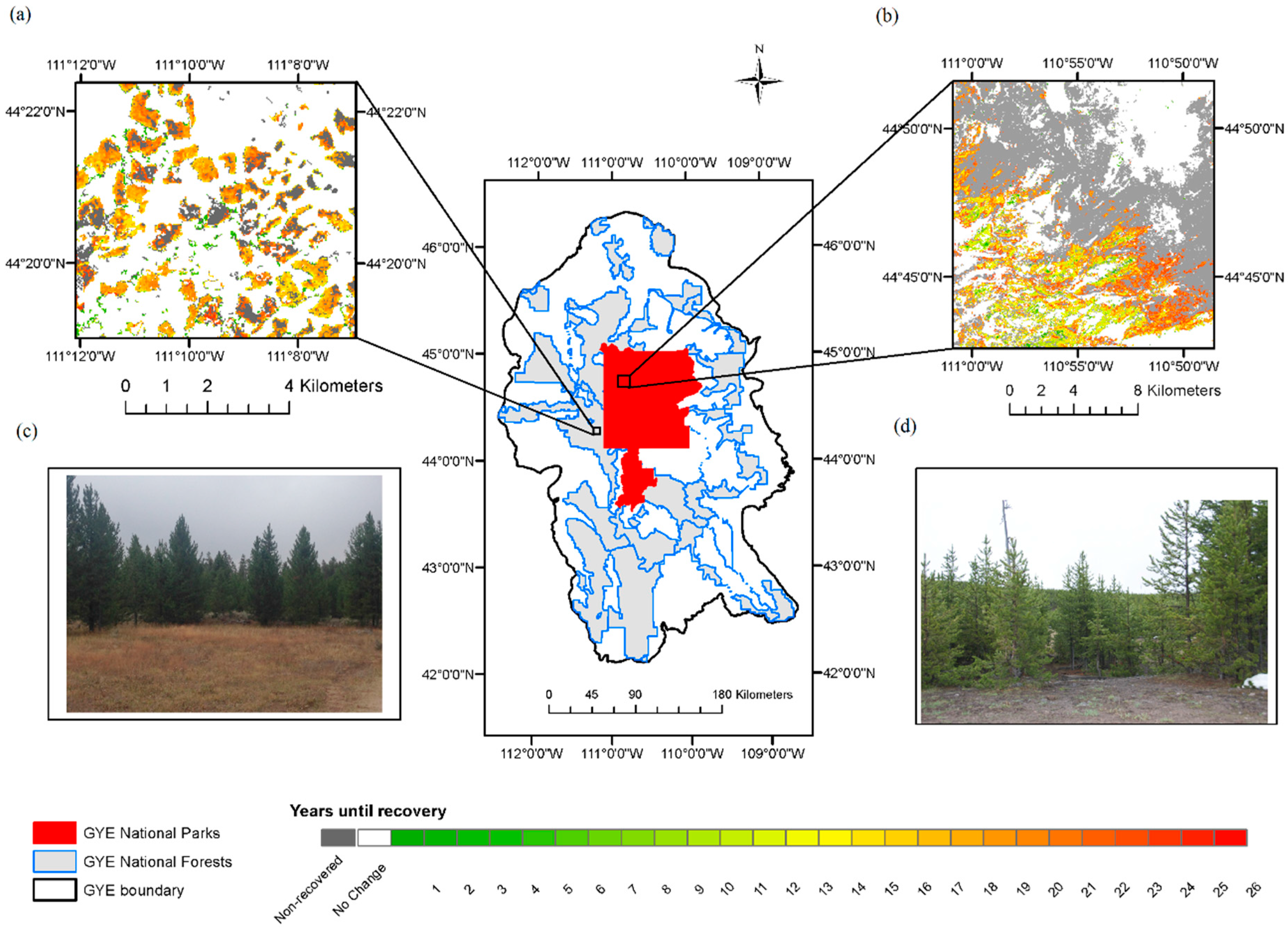
2. Study Area
3. Materials and Methods
3.1. LTSS Assembling
3.2. Forest Disturbance and Recovery Mapping
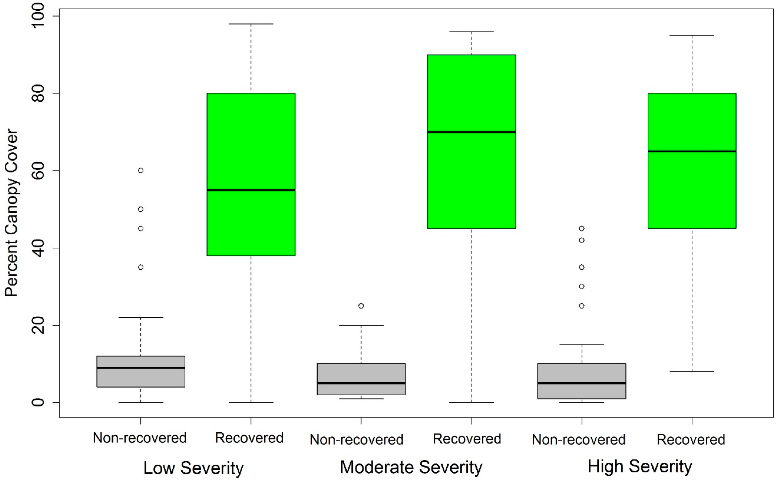
3.3. Validation of Recovery Products
3.4. Spatiotemporal Recovery Pattern Analysis
4. Results
4.1. Accuracy of the Forest Spectral Recovery/No-Detectable-Recovery (RNR) Maps
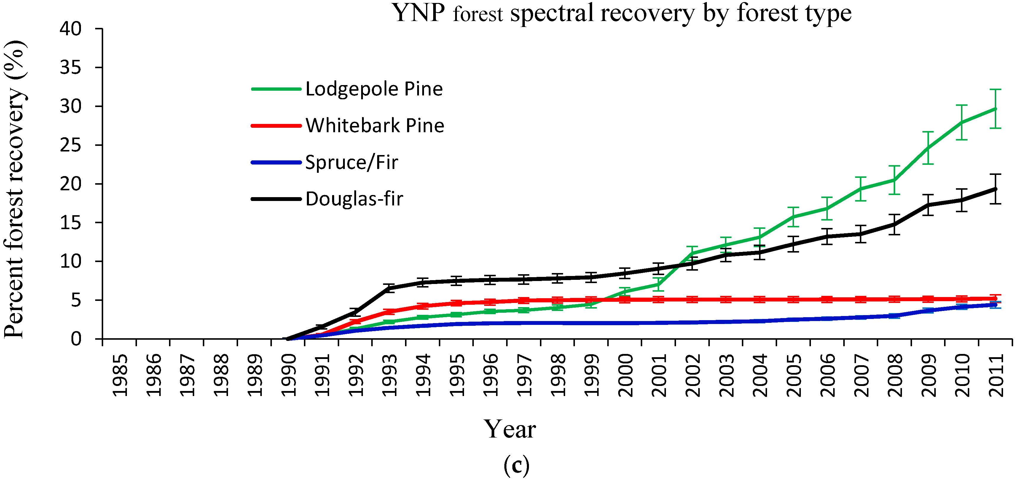
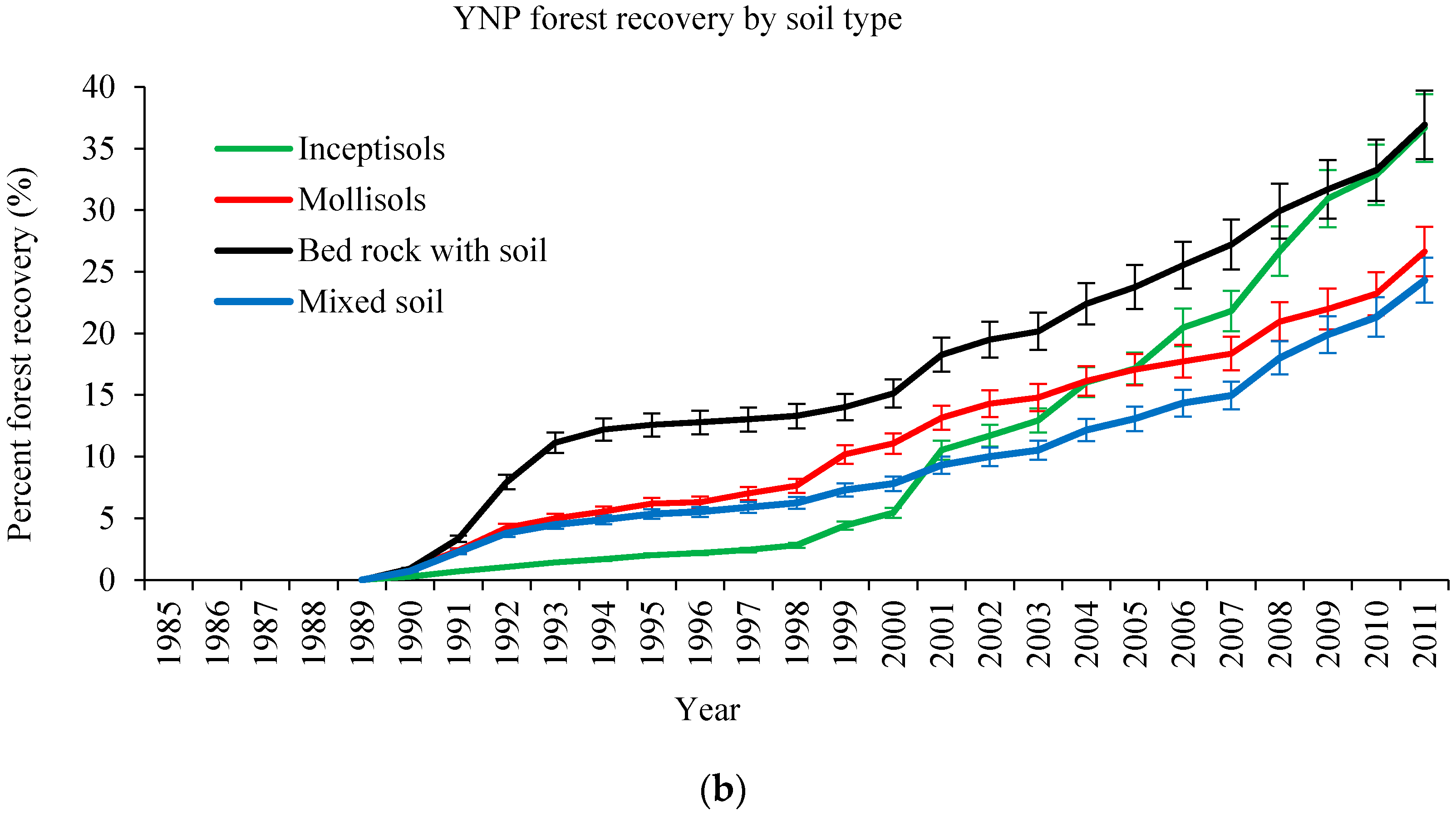
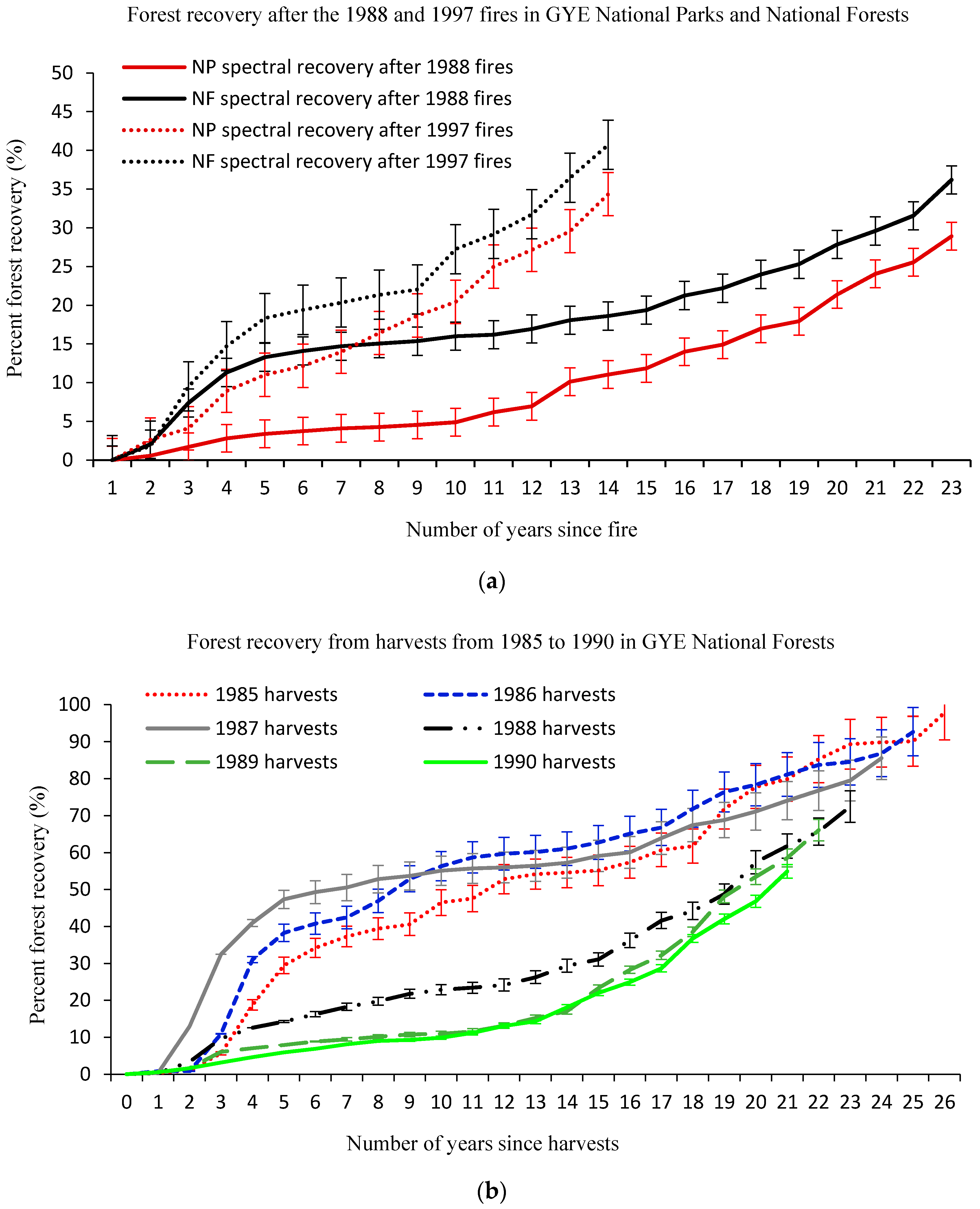
4.2. Spectral Recovery Patterns by Ownership, Disturbance Type, Forest and Soil Types in the GYE
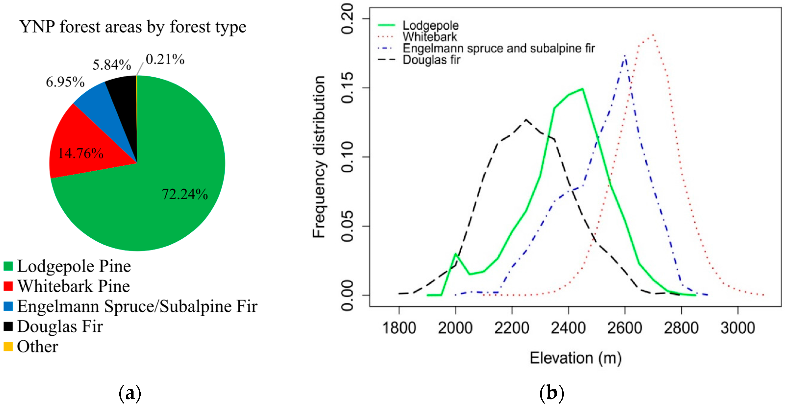
4.3. Spectral Recovery Patterns along Environmental Gradients in the Yellowstone National Park
5. Discussion
5.1. Challenges in Time Series Forest Recovery Mapping
5.2. Spatial and Temporal Pattern Analysis of Forest Spectral Recovery in the GYE
6. Conclusions
Supplementary Materials
Acknowledgments
Author Contributions
Conflicts of Interest
Abbreviations
| GYE | Greater Yellowstone Ecosystem |
| YNP | Yellowstone National Park |
| NPs | National Parks |
| NFs | National Forests |
| WAs | Wilderness Areas |
| VCT | Vegetation Change Tracker |
| IFZ | Integrated Forest z-score |
References
- Parmenter, A.W.; Hansen, A.; Kennedy, R.E.; Cohen, W.; Langner, U.; Lawrence, R.; Maxwell, B.; Gallant, A.; Aspinall, R. Land use and land cover change in the greater yellowstone ecosystem: 1975–1995. Ecol. Appl. 2003, 13, 687–703. [Google Scholar] [CrossRef]
- Zhao, F.; Huang, C.; Zhu, Z. Use of vegetation change tracker and support vector machine to map disturbance types in greater yellowstone ecosystems in a 1984–2010 Landsat time series. IEEE Geosci. Remote Sens. Lett. 2015, 12, 1650–1654. [Google Scholar] [CrossRef]
- Pan, Y.; Birdsey, R.A.; Fang, J.; Houghton, R.; Kauppi, P.E.; Kurz, W.A.; Phillips, O.L.; Shvidenko, A.; Lewis, S.L.; Canadell, J.G. A large and persistent carbon sink in the world’s forests. Science 2011, 333, 988–993. [Google Scholar] [CrossRef] [PubMed]
- Houghton, R.A.; Hackler, J.L.; Lawrence, K. The us carbon budget: Contributions from land-use change. Science 1999, 285, 574–578. [Google Scholar] [CrossRef] [PubMed]
- Goetz, S.J.; Bond-Lamberty, B.; Law, B.E.; Hicke, J.; Huang, C.; Houghton, R.; McNulty, S.; O’Halloran, T.; Harmon, M.; Meddens, A. Observations and assessment of forest carbon dynamics following disturbance in North America. J. Geophys. Res. Biogeosci. 2012, 117, 1–17. [Google Scholar] [CrossRef]
- Liu, S.; Bond-Lamberty, B.; Hicke, J.; Vargas, R.; Zhao, S.; Chen, J.; Edburg, S.; Hu, Y.; Liu, J.; McGuire, A.; et al. Simulating the impacts of disturbances on forest carbon cycling in North America: Processes, data, models, and challenges. J. Geophys. Res. Biogeosci. 2011, 116, 1–22. [Google Scholar] [CrossRef]
- Bartels, S.F.; Chen, H.Y.H.; Wulder, M.A.; White, J.C. Trends in post-disturbance recovery rates of Canada’s forests following wildfire and harvest. For. Ecol. Manag. 2016, 361, 194–207. [Google Scholar] [CrossRef]
- Schroeder, T.A.; Cohen, W.B.; Yang, Z. Patterns of forest regrowth following clearcutting in western Oregon as determined from a Landsat time-series. For. Ecol. Manag. 2007, 243, 259–273. [Google Scholar] [CrossRef]
- Potter, C.; Li, S.; Huang, S.; Crabtree, R.L. Analysis of sapling density regeneration in Yellowstone National Park with hyperspectral remote sensing data. Remote Sens. Environ. 2012, 121, 61–68. [Google Scholar] [CrossRef]
- Frolking, S.; Palace, M.W.; Clark, D.B.; Chambers, J.Q.; Shugart, H.H.; Hurtt, G.C. Forest disturbance and recovery: A general review in the context of spaceborne remote sensing of impacts on aboveground biomass and canopy structure. J. Geophys. Res. Biogeosci. 2009, 114, 1–27. [Google Scholar] [CrossRef]
- Kennedy, R.E.; Yang, Z.; Cohen, W.B.; Pfaff, E.; Braaten, J.; Nelson, P. Spatial and temporal patterns of forest disturbance and regrowth within the area of the Northwest Forest plan. Remote Sens. Environ. 2012, 122, 117–133. [Google Scholar] [CrossRef]
- Vogelmann, J.E.; Gallant, A.L.; Shi, H.; Zhu, Z. Perspectives on monitoring gradual change across the continuity of Landsat sensors using time-series data. Remote Sens. Environ. 2016, 185, 258–270. [Google Scholar] [CrossRef]
- Vogelmann, J.E.; Xian, G.; Homer, C.; Tolk, B. Monitoring gradual ecosystem change using Landsat time series analyses: Case studies in selected forest and rangeland ecosystems. Remote Sens. Environ. 2012, 122, 92–105. [Google Scholar] [CrossRef]
- Hansen, M.C.; Potapov, P.V.; Moore, R.; Hancher, M.; Turubanova, S.; Tyukavina, A.; Thau, D.; Stehman, S.; Goetz, S.; Loveland, T. High-resolution global maps of 21st-century forest cover change. Science 2013, 342, 850–853. [Google Scholar] [CrossRef] [PubMed]
- Lentile, L.B.; Holden, Z.A.; Smith, A.M.S.; Falkowski, M.J.; Hudak, A.T.; Morgan, P.; Lewis, S.A.; Gessler, P.E.; Benson, N.C. Remote sensing techniques to assess active fire characteristics and post-fire effects. Int. J. Wildland Fire 2006, 15, 319–345. [Google Scholar] [CrossRef]
- Chu, T.; Guo, X. Remote sensing techniques in monitoring post-fire effects and patterns of forest recovery in boreal forest regions: A review. Remote Sens. 2013, 6, 470–520. [Google Scholar] [CrossRef]
- Tanase, M.; de la Riva, J.; Santoro, M.; Pérez-Cabello, F.; Kasischke, E. Sensitivity of sar data to post-fire forest regrowth in Mediterranean and boreal forests. Remote Sens. Environ. 2011, 115, 2075–2085. [Google Scholar] [CrossRef]
- Kane, V.R.; North, M.P.; Lutz, J.A.; Churchill, D.J.; Roberts, S.L.; Smith, D.F.; McGaughey, R.J.; Kane, J.T.; Brooks, M.L. Assessing fire effects on forest spatial structure using a fusion of Landsat and airborne lidar data in Yosemite National Park. Remote Sens. Environ. 2014, 151, 89–101. [Google Scholar] [CrossRef]
- Asner, G.P.; Knapp, D.E.; Broadbent, E.N.; Oliveira, P.J.C.; Keller, M.; Silva, J.N. Selective logging in the Brazilian Amazon. Science 2005, 310, 480–482. [Google Scholar] [CrossRef] [PubMed]
- Souza, C.M.; Roberts, D.A.; Cochrane, M.A. Combining spectral and spatial information to map canopy damage from selective logging and forest fires. Remote Sens. Environ. 2005, 98, 329–343. [Google Scholar] [CrossRef]
- Andersen, H.-E.; Reutebuch, S.E.; McGaughey, R.J.; D’Oliveira, M.V.N.; Keller, M. Monitoring selective logging in western Amazonia with repeat lidar flights. Remote Sens. Environ. 2014, 151, 157–165. [Google Scholar] [CrossRef]
- Schroeder, T.A.; Wulder, M.A.; Healey, S.P.; Moisen, G.G. Detecting post-fire salvage logging from Landsat change maps and national fire survey data. Remote Sens. Environ. 2012, 122, 166–174. [Google Scholar] [CrossRef]
- Meng, R.; Dennison, P.E.; Huang, C.; Moritz, M.A.; D’Antonio, C. Effects of fire severity and post-fire climate on short-term vegetation recovery of mixed-conifer and red fir forests in the Sierra Nevada mountains of California. Remote Sens. Environ. 2015, 171, 311–325. [Google Scholar] [CrossRef]
- Roy, D.P.; Wulder, M.A.; Loveland, T.R.; Woodcock, C.E.; Allen, R.G.; Anderson, M.C.; Helder, D.; Irons, J.R.; Johnson, D.M.; Kennedy, R. Landsat-8: Science and product vision for terrestrial global change research. Remote Sens. Environ. 2014, 145, 154–172. [Google Scholar] [CrossRef]
- Zhu, Z.; Woodcock, C.E. Continuous change detection and classification of land cover using all available Landsat data. Remote Sens. Environ. 2014, 144, 152–171. [Google Scholar] [CrossRef]
- Cohen, W.B.; Yang, Z.; Stehman, S.V.; Schroeder, T.A.; Bell, D.M.; Masek, J.G.; Huang, C.; Meigs, G.W. Forest disturbance across the conterminous united states from 1985–2012: The emerging dominance of forest decline. For. Ecol. Manag. 2016, 360, 242–252. [Google Scholar] [CrossRef]
- Gong, P.; Xu, B. Remote sensing of forests over time. In Remote Sensing of Forest Environments; Springer: Boston, MA, USA, 2003; pp. 301–333. [Google Scholar]
- Healey, S.P.; Cohen, W.B.; Zhiqiang, Y.; Krankina, O.N. Comparison of tasseled cap-based Landsat data structures for use in forest disturbance detection. Remote Sens. Environ. 2005, 97, 301–310. [Google Scholar] [CrossRef]
- Schroeder, T.A.; Wulder, M.A.; Healey, S.P.; Moisen, G.G. Mapping wildfire and clearcut harvest disturbances in boreal forests with Landsat time series data. Remote Sens. Environ. 2011, 115, 1421–1433. [Google Scholar] [CrossRef]
- Hilker, T.; Wulder, M.A.; Coops, N.C.; Linke, J.; McDermid, G.; Masek, J.G.; Gao, F.; White, J.C. A new data fusion model for high spatial- and temporal-resolution mapping of forest disturbance based on Landsat and MODIS. Remote Sens. Environ. 2009, 113, 1613–1627. [Google Scholar] [CrossRef]
- Griffiths, P.; Kuemmerle, T.; Baumann, M.; Radeloff, V.C.; Abrudan, I.V.; Lieskovsky, J.; Munteanu, C.; Ostapowicz, K.; Hostert, P. Forest disturbances, forest recovery, and changes in forest types across the Carpathian ecoregion from 1985 to 2010 based on Landsat image composites. Remote Sens. Environ. 2014, 151, 72–88. [Google Scholar] [CrossRef]
- Hermosilla, T.; Wulder, M.A.; White, J.C.; Coops, N.C.; Hobart, G.W.; Campbell, L.B. Mass data processing of time series Landsat imagery: Pixels to data products for forest monitoring. Int. J. Digit. Earth 2016, 9, 1–20. [Google Scholar] [CrossRef]
- Huang, C.; Kim, S.; Altstatt, A.; Townshend, J.R.G.; Davis, P.; Song, K.; Tucker, C.J.; Rodas, O.; Yanosky, A.; Clay, R.; et al. Rapid loss of Paraguay’s Atlantic forest and the status of protected areas—A Landsat assessment. Remote Sens. Environ. 2007, 106, 460–466. [Google Scholar] [CrossRef]
- Potapov, P.; Hansen, M.C.; Stehman, S.V.; Pittman, K.; Turubanova, S. Gross forest cover loss in temperate forests: Biome-wide monitoring results using MODIS and Landsat data. J. Appl. Remote Sens. 2009, 3, 033569. [Google Scholar] [CrossRef]
- Wulder, M.; White, J.; Alvarez, F.; Han, T.; Rogan, J.; Hawkes, B. Characterizing boreal forest wildfire with multi-temporal Landsat and lidar data. Remote Sens. Environ. 2009, 113, 1540–1555. [Google Scholar] [CrossRef]
- Verbesselt, J.; Hyndman, R.; Newnham, G.; Culvenor, D. Detecting trend and seasonal changes in satellite image time series. Remote Sens. Environ. 2010, 114, 106–115. [Google Scholar] [CrossRef]
- DeVries, B.; Verbesselt, J.; Kooistra, L.; Herold, M. Robust monitoring of small-scale forest disturbances in a tropical montane forest using Landsat time series. Remote Sens. Environ. 2015, 161, 107–121. [Google Scholar] [CrossRef]
- Zhu, Z.; Woodcock, C.E.; Olofsson, P. Continuous monitoring of forest disturbance using all available Landsat imagery. Remote Sens. Environ. 2012, 122, 75–91. [Google Scholar] [CrossRef]
- Baumann, M.; Ozdogan, M.; Kuemmerle, T.; Wendland, K.J.; Esipova, E.; Radeloff, V.C. Using the Landsat record to detect forest-cover changes during and after the collapse of the Soviet Union in the temperate zone of European Russia. Remote Sens. Environ. 2012, 124, 174–184. [Google Scholar] [CrossRef]
- Kennedy, R.E.; Yang, Z.; Cohen, W.B. Detecting trends in forest disturbance and recovery using yearly Landsat time series: 1. LandTrendr—Temporal segmentation algorithms. Remote Sens. Environ. 2010, 114, 2897–2910. [Google Scholar] [CrossRef]
- Trumbore, S.; Brando, P.; Hartmann, H. Forest health and global change. Science 2015, 349, 814–818. [Google Scholar] [CrossRef] [PubMed]
- Turner, M.G.; Whitby, T.G.; Tinker, D.B.; Romme, W.H. Twenty-four years after the Yellowstone fires: Are postfire lodgepole pine stands converging in structure and function? Ecology 2016, 97, 1260–1273. [Google Scholar] [CrossRef] [PubMed]
- Huang, C.; Goward, S.N.; Masek, J.G.; Thomas, N.; Zhu, Z.; Vogelmann, J.E. An automated approach for reconstructing recent forest disturbance history using dense Landsat time series stacks. Remote Sens. Environ. 2010, 114, 183–198. [Google Scholar] [CrossRef]
- Huang, C.; Goward, S.N.; Masek, J.G.; Gao, F.; Vermote, E.F.; Thomas, N.; Schleeweis, K.; Kennedy, R.E.; Zhu, Z.; Eidenshink, J.C. Development of time series stacks of landsat images for reconstructing forest disturbance history. Int. J. Digit. Earth 2009, 2, 195–218. [Google Scholar] [CrossRef]
- Thomas, N.E.; Huang, C.; Goward, S.N.; Powell, S.; Rishmawi, K.; Schleeweis, K.; Hinds, A. Validation of North American forest disturbance dynamics derived from Landsat time series stacks. Remote Sens. Environ. 2011, 115, 19–32. [Google Scholar] [CrossRef]
- Huang, C.; Schleeweis, K.; Thomas, N.; Goward, S.N. Forest dynamics within and around the Olympic National Park assessed using time series Landsat observations. In Remote Sensing of Protected Lands; Wang, Y., Ed.; Taylor & Francis: London, UK, 2011; pp. 71–93. [Google Scholar]
- Huang, C.; Goward, S.N.; Schleeweis, K.; Thomas, N.; Masek, J.G.; Zhu, Z. Dynamics of national forests assessed using the Landsat record: Case studies in eastern U.S. Remote Sens. Environ. 2009, 113, 1430–1442. [Google Scholar] [CrossRef]
- Huang, C.; Ling, P.-Y.; Zhu, Z. North Carolina’s forest disturbance and timber production assessed using time series Landsat observations. Int. J. Digit. Earth 2015, 8, 1–41. [Google Scholar] [CrossRef]
- Landenburger, L.; Lawrence, R.L.; Podruzny, S.; Schwartz, C.C. Mapping regional distribution of a single tree species: Whitebark pine in the greater Yellowstone ecosystem. Sensors 2008, 8, 4983–4994. [Google Scholar] [CrossRef]
- Alexander, R.R. Silviculture of central and southern Rocky Mountain forests: A summary of the status of our knowledge by timber types. In Silviculture of Subalpine Forests in the Central and Southern Rocky Mountains: The Status of Our Knowledge; Rocky Mountain Forest and Range Experiment Station: Fort Collins, CO, USA, 1974; pp. 1–35. [Google Scholar]
- Alexander, R.R.; Edminster, C.B. Lodgepole pine management in the central Rocky mountains. J. For. 1980, 78, 196–201. [Google Scholar]
- Hansen, A.J.; Rotella, J.J.; Kraska, M.P.; Brown, D. Spatial patterns of primary productivity in the greater Yellowstone ecosystem. Lands. Ecol. 2000, 15, 505–522. [Google Scholar] [CrossRef]
- Robichaud, P.R.; Beyers, J.L.; Neary, D.G. Evaluating the Effectiveness of Postfire Rehabilitation Treatments; U.S. Department of Agricul, Forest Service: Fort Collins, CO, USA, 2000; p. 85.
- Harvey, B.J.; Donato, D.C.; Romme, W.H.; Turner, M.G. Fire severity and tree regeneration following bark beetle outbreaks: The role of outbreak stage and burning conditions. Ecol. Appl. 2014, 24, 1608–1625. [Google Scholar] [CrossRef]
- Turner, M.G.; Romme, W.H.; Gardner, R.H.; Hargrove, W.W. Effects of fire size and pattern on early succession in Yellowstone National Park. Ecol. Monogr. 1997, 67, 411–433. [Google Scholar] [CrossRef]
- Franks, S.; Masek, J.G.; Turner, M.G. Monitoring forest regrowth following large scale fire using satellite data—A case study of Yellowstone National Park, USA. Eur. J. Remote Sens. 2013, 46, 551–569. [Google Scholar] [CrossRef]
- Schoennagel, T.; Turner, M.G.; Romme, W.H. The influence of fire interval and serotiny on postfire lodgepole pine density in Yellowstone National Park. Ecology 2003, 84, 2967–2978. [Google Scholar] [CrossRef]
- Romme, W.H.; Boyce, M.S.; Gresswell, R.; Merrill, E.H.; Minshall, G.W.; Whitlock, C.; Turner, M.G. Twenty years after the 1988 Yellowstone fires: Lessons about disturbance and ecosystems. Ecosystems 2011, 14, 1196–1215. [Google Scholar] [CrossRef]
- Marston, R.A.; Anderson, J.E. Watersheds and vegetation of the greater Yellowstone ecosystem. Conserv. Biol. 1991, 5, 338–346. [Google Scholar] [CrossRef]
- Renkin, R.A.; Despain, D.G. Fuel moisture, forest type, and lightning-caused fire in Yellowstone National Park. Can. J. For. Res. 1992, 22, 37–45. [Google Scholar] [CrossRef]
- Masek, J.G.; Vermote, E.F.; Saleous, N.E.; Wolfe, R.; Hall, F.G.; Huemmrich, K.F.; Gao, F.; Kutler, J.; Lim, T.-K. A Landsat surface reflectance dataset for North America, 1990–2000. IEEE Geosci. Remote Sens. Lett. 2006, 3, 68–72. [Google Scholar] [CrossRef]
- Huang, C.; Thomas, N.; Goward, S.N.; Masek, J.G.; Zhu, Z.; Townshend, J.R.; Vogelmann, J.E. Automated masking of cloud and cloud shadow for forest change analysis using Landsat images. Int. J. Remote Sens. 2010, 31, 5449–5464. [Google Scholar] [CrossRef]
- Huete, A.R.; Liu, H.Q.; Batchily, K.; van Leeuwen, W. A comparison of vegetation indices over a global set of TM images for EOS-MODIS. Remote Sens. Environ. 1997, 59, 440–451. [Google Scholar] [CrossRef]
- Kogan, F. Application of vegetation index and brightness temperature for drought detection. Adv. Space Res. 1995, 15, 91–100. [Google Scholar] [CrossRef]
- Huang, C.; Song, K.; Kim, S.; Townshend, J.R.G.; Davis, P.; Masek, J.; Goward, S.N. Use of a dark object concept and support vector machines to automate forest cover change analysis. Remote Sens. Environ. 2008, 112, 970–985. [Google Scholar] [CrossRef]
- Miller, J.D.; Thode, A.E. Quantifying burn severity in a heterogeneous landscape with a relative version of the delta normalized burn ratio (DNBR). Remote Sens. Environ. 2007, 109, 66–80. [Google Scholar] [CrossRef]
- Miller, J.D.; Knapp, E.E.; Key, C.H.; Skinner, C.N.; Isbell, C.J.; Creasy, R.M.; Sherlock, J.W. Calibration and validation of the relative differenced normalized burn ratio (RDNBR) to three measures of fire severity in the Sierra Nevada and Klamath mountains, California, USA. Remote Sens. Environ. 2009, 113, 645–656. [Google Scholar] [CrossRef]
- Moran, P.A.P. Notes on continuous stochastic phenomena. Biometrika 1950, 37, 17–23. [Google Scholar] [CrossRef] [PubMed]
- Li, H.; Calder, C.A.; Cressie, N. Beyond Moran’s I: Testing for spatial dependence based on the spatial autoregressive model. Geogr. Anal. 2007, 39, 357–375. [Google Scholar] [CrossRef]
- Westerling, A.; Turner, M.; Smithwick, E.; Romme, W.; Ryan, M. Continued warming could transform greater Yellowstone fire regimes by mid-21st century. Proc. Natl. Acad. Sci. USA 2011, 108, 13165–13170. [Google Scholar] [CrossRef] [PubMed]
- Turner, M.G.; Romme, W.H.; Tinker, D.B. Surprises and lessons from the 1988 Yellowstone fires. Front. Ecol. Environ. 2003, 1, 351–358. [Google Scholar] [CrossRef]
- Attiwill, P.M. The disturbance of forest ecosystems: The ecological basis for conservative management. For. Ecol. Manag. 1994, 63, 247–300. [Google Scholar] [CrossRef]
- Dolan, K.; Masek, J.G.; Huang, C.; Sun, G. Regional forest growth rates measured by combining ICESat GLAS and Landsat data. J. Geophys. Res. Biogeosci. 2009, 114, 1–7. [Google Scholar] [CrossRef]
- Helmer, E.H.; Lefsky, M.A.; Roberts, D.A. Biomass accumulation rates of amazonian secondary forest and biomass of old-growth forests from Landsat time series and the geoscience laser altimeter system. J. Appl. Remote Sens. 2009, 3, 033505. [Google Scholar]
- Helmer, E.H.; Ruzycki, T.S.; Wunderle, J.M.; Vogesser, S.; Ruefenacht, B.; Kwit, C.; Ewert, D.N. Mapping tropical dry forest height, foliage height profiles and disturbance type and age with a time series of cloud-cleared Landsat and ali image mosaics to characterize avian habitat. Remote Sens. Environ. 2010, 114, 2457–2473. [Google Scholar] [CrossRef]
- Frazier, R.J.; Coops, N.C.; Wulder, M.A. Boreal shield forest disturbance and recovery trends using Landsat time series. Remote Sens. Environ. 2015, 170, 317–327. [Google Scholar] [CrossRef]
- Pickell, P.D.; Hermosilla, T.; Frazier, R.J.; Coops, N.C.; Wulder, M.A. Forest recovery trends derived from Landsat time series for North American boreal forests. Int. J. Remote Sens. 2016, 37, 138–149. [Google Scholar] [CrossRef]
- Wijdeven, S.M.; Kuzee, M.E. Seed availability as a limiting factor in forest recovery processes in Costa Rica. Restor. Ecol. 2000, 8, 414–424. [Google Scholar] [CrossRef]
- Savage, M.; Brown, P.M.; Feddema, J. The role of climate in a pine forest regeneration pulse in the southwestern United States. Ecoscience 1996, 3, 310–318. [Google Scholar] [CrossRef]
- Simpson, R.; Leck, M.A.; Parker, V. Seed banks: General concepts and methodological issues. Ecol. Soil Seed Banks 1989, 1, 3–8. [Google Scholar]
- Frank, D.A.; McNaughton, S.J. The ecology of plants, large mammalian herbivores, and drought in Yellowstone National Park. Ecology 1992, 73, 2043–2058. [Google Scholar] [CrossRef]
- Li, A.; Huang, C.; Sun, G.; Shi, H.; Toney, C.; Zhu, Z.; Rollins, M.G.; Goward, S.N.; Masek, J.G. Modeling the height of young forests regenerating from recent disturbances in Mississippi using Landsat and ICESat data. Remote Sens. Environ. 2011, 115, 1837–1849. [Google Scholar] [CrossRef]
- Romme, W.H.; Knight, D.H. Fire frequency and subalpine forest succession along a topographic gradient in Wyoming. Ecology 1981, 62, 319–326. [Google Scholar] [CrossRef]
- Turner, M.G.; Romme, W.H.; Gardner, R.H. Prefire heterogeneity, fire severity, and early postfire plant reestablishment in subalpine forests of Yellowstone National Park, Wyoming. Int. J. Wildland Fire 1999, 9, 21–36. [Google Scholar] [CrossRef]
- Turner, M.G.; Baker, W.L.; Peterson, C.J.; Peet, R.K. Factors influencing succession: Lessons from large, infrequent natural disturbances. Ecosystems 1998, 1, 511–523. [Google Scholar] [CrossRef]


| Post-Fire Spectral Recovery Validation Results | |||||
| Reference | |||||
| Recovered (Tree Cover > 10%) | No-Detectable-Recovery (Tree Cover ≤ 10%) | Row Total | User’s Accuracy | ||
| Map | Spectrally recovered | 0.19 | 0.07 | 0.26 | 0.75 |
| No-detectable-recovery | 0.13 | 0.61 | 0.74 | 0.82 | |
| Column total | 0.32 | 0.68 | 1.00 | ||
| Producer’s Accuracy | 0.59 | 0.90 | |||
| Overall Accuracy | 0.80 | ||||
| Post-Harvest Spectral Recovery Validation Results | |||||
| Reference | |||||
| Recovered (Tree Cover > 10%) | No-Detectable-Recovery (Tree Cover ≤ 10%) | Row Total | User’s Accuracy | ||
| Map | Spectrally recovered | 0.69 | 0.02 | 0.71 | 0.97 |
| No-detectable-recovery | 0.12 | 0.17 | 0.29 | 0.58 | |
| Column total | 0.81 | 0.19 | 1.00 | ||
| Producer’s Accuracy | 0.85 | 0.89 | |||
| Overall Accuracy | 0.86 | ||||
| Lodgepole Pine (72% of Area) | |||||
| Reference | |||||
| Recovered (Tree Cover > 10%) | No-Detectable-Recovery (Tree Cover ≤ 10%) | Row Total | User’s Accuracy | ||
| Map | Spectrally recovered | 0.28 | 0.02 | 0.30 | 0.94 |
| No-detectable-recovery | 0.15 | 0.55 | 0.70 | 0.78 | |
| Column total | 0.43 | 0.57 | 1.00 | ||
| Producer’s Accuracy | 0.65 | 0.97 | |||
| Overall Accuracy | 0.83 | ||||
| Whitebark Pine (15% of Area) | |||||
| Reference | |||||
| Recovered (Tree Cover > 10%) | No-Detectable-Recovery (Tree Cover ≤ 10%) | Row Total | User’s Accuracy | ||
| Map | Spectrally recovered | 0.01 | 0.04 | 0.05 | 0.18 |
| No-detectable-recovery | 0.08 | 0.87 | 0.95 | 0.92 | |
| Column total | 0.09 | 0.91 | 1.00 | ||
| Producer’s Accuracy | 0.11 | 0.95 | |||
| Overall Accuracy | 0.88 | ||||
| Douglas Fir (7.1% of Area) | |||||
| Reference | |||||
| Recovered (Tree Cover > 10%) | No-Detectable-Recovery (Tree Cover ≤ 10%) | Row Total | User’s Accuracy | ||
| Map | Spectrally recovered | 0.17 | 0.04 | 0.22 | 0.80 |
| No-detectable-recovery | 0.19 | 0.59 | 0.78 | 0.75 | |
| Column total | 0.37 | 0.63 | 1.00 | ||
| Producer’s Accuracy | 0.47 | 0.93 | |||
| Overall Accuracy | 0.76 | ||||
| Engelmann Spruce and Subalpine Fir (5.9% of Area) | |||||
| Reference | |||||
| Recovered (Tree Cover > 10%) | No-Detectable-Recovery (Tree Cover ≤ 10%) | Row Total | User’s Accuracy | ||
| Map | Spectrally recovered | 0.03 | 0.02 | 0.05 | 0.68 |
| No-detectable-recovery | 0.15 | 0.80 | 0.95 | 0.84 | |
| Column total | 0.18 | 0.82 | 1.00 | ||
| Producer’s Accuracy | 0.18 | 0.98 | |||
| Overall Accuracy | 0.84 | ||||
© 2016 by the authors; licensee MDPI, Basel, Switzerland. This article is an open access article distributed under the terms and conditions of the Creative Commons Attribution (CC-BY) license (http://creativecommons.org/licenses/by/4.0/).
Share and Cite
Zhao, F.R.; Meng, R.; Huang, C.; Zhao, M.; Zhao, F.A.; Gong, P.; Yu, L.; Zhu, Z. Long-Term Post-Disturbance Forest Recovery in the Greater Yellowstone Ecosystem Analyzed Using Landsat Time Series Stack. Remote Sens. 2016, 8, 898. https://doi.org/10.3390/rs8110898
Zhao FR, Meng R, Huang C, Zhao M, Zhao FA, Gong P, Yu L, Zhu Z. Long-Term Post-Disturbance Forest Recovery in the Greater Yellowstone Ecosystem Analyzed Using Landsat Time Series Stack. Remote Sensing. 2016; 8(11):898. https://doi.org/10.3390/rs8110898
Chicago/Turabian StyleZhao, Feng R., Ran Meng, Chengquan Huang, Maosheng Zhao, Feng A. Zhao, Peng Gong, Le Yu, and Zhiliang Zhu. 2016. "Long-Term Post-Disturbance Forest Recovery in the Greater Yellowstone Ecosystem Analyzed Using Landsat Time Series Stack" Remote Sensing 8, no. 11: 898. https://doi.org/10.3390/rs8110898
APA StyleZhao, F. R., Meng, R., Huang, C., Zhao, M., Zhao, F. A., Gong, P., Yu, L., & Zhu, Z. (2016). Long-Term Post-Disturbance Forest Recovery in the Greater Yellowstone Ecosystem Analyzed Using Landsat Time Series Stack. Remote Sensing, 8(11), 898. https://doi.org/10.3390/rs8110898