Article

Mapping Distinct Forest Types Improves Overall Forest Identification Based on Multi-Spectral Landsat Imagery for Myanmar’s Tanintharyi Region

1
Conservation Ecology Center/Myanmar Program, Smithsonian Conservation Biology Institute, 1500 Remount Road, Front Royal, VA 22630, USA
2
Fauna & Flora International, 35 Shan Kone Street, San Chaung Township, Yangon 11111, Myanmar
*
Author to whom correspondence should be addressed.
Remote Sens. 2016, 8(11), 882; https://doi.org/10.3390/rs8110882
Submission received: 31 July 2016 / Revised: 29 September 2016 / Accepted: 21 October 2016 / Published: 25 October 2016

Abstract

:
We investigated the use of multi-spectral Landsat OLI imagery for delineating mangrove, lowland evergreen, upland evergreen and mixed deciduous forest types in Myanmar’s Tanintharyi Region and estimated the extent of degraded forest for each unique forest type. We mapped a total of 16 natural and human land use classes using both a Random Forest algorithm and a multivariate Gaussian model while considering scenarios with all natural forest classes grouped into a single intact or degraded category. Overall, classification accuracy increased for the multivariate Gaussian model with the partitioning of intact and degraded forest into separate forest cover classes but slightly decreased based on the Random Forest classifier. Natural forest cover was estimated to be 80.7% of total area in Tanintharyi. The most prevalent forest types are upland evergreen forest (42.3% of area) and lowland evergreen forest (21.6%). However, while just 27.1% of upland evergreen forest was classified as degraded (on the basis of canopy cover <80%), 66.0% of mangrove forest and 47.5% of the region’s biologically-rich lowland evergreen forest were classified as degraded. This information on the current status of Tanintharyi’s unique forest ecosystems and patterns of human land use is critical to effective conservation strategies and land-use planning.

Graphical Abstract

1. Introduction

The complex geological and bioclimatic history of Southeast Asia has resulted in an exceptionally rich biodiversity [1] and some of the highest concentrations of endemic species in the world [2]. The floristically-distinct forest types that occur in the region vary in their species assemblages, vulnerability to habitat conversion or degradation, conservation value, and representation within protected area networks [3,4]. Forests that are accessible and occur in areas with high human population densities are especially vulnerable to degradation and deforestation. As a result, the region’s remaining forest cover predominantly occurs at high elevations or in areas that are difficult to access due to steep terrain [5]. Lowland evergreen forests have experienced especially high rates of forest loss [6,7]. Similarly, mangrove forests occur exclusively in coastal areas and are undergoing rapid conversion to agriculture [8]. Due to the unique threats faced by different forest types, conservation strategies and risk assessments in the region should be based on an accurate understanding of current forest distributions and knowledge of where forest loss and degradation are taking place.
Although the extent of forest degradation in some landscapes may be much larger than the extent of outright forest loss (e.g., [9,10]), forest degradation is more difficult to monitor with remote sensing techniques than outright deforestation. Various approaches have been applied to the mapping of forest degradation, such as the analysis of time series data (e.g., [11]), use of canopy cover loss as an indicator of degradation (e.g., [12,13,14]), or mapping of secondary degradation indicators such as log landings and logging roads (e.g., [15]). Assessing forest degradation in continental Southeast Asia is particularly challenging due to variation among natural forest types in their physical structure and seasonal patterns of canopy cover that range from evergreen to fully deciduous [5]. This region has a monsoon climate with a distinct wet season (May–October) that corresponds with elevated vegetation growth [16]. The dry season (November–March) provides greater availability of cloud-free satellite imagery at a time when reduced canopy cover may indicate either forest degradation or the presence of deciduous tree species in their annual leaf-off period. Thus, distinguishing between deciduous forest and canopy thinning due to degradation is an important challenge in continental Southeast Asia and it has been suggested that single-date mapping of forest degradation based on canopy cover may be unreliable without matching data for specific sites in intact condition [5].
However, fairly subtle differences in forest type may be resolvable using medium-resolution satellite imagery. Recent studies have demonstrated that local floristic differences in tropical forests can be effectively identified using a combination of medium-resolution multi-spectral (e.g., Landsat) and topographic data [17,18,19,20,21]. Scaling these approaches to broader landscapes may be problematic if this results in increased spectral variability within forest classes and reduced ability to distinguish among them. This may be due to factors such as forest disturbance, topographic shadowing, or differences among scenes in a mosaicked image [22]. Sometimes these limitations are avoided by assessments and studies that focus on mapping a single forest type of interest (e.g., [3,23]), yet country- and regional-level conservation planning often require comprehensive assessments of all forest types and their associated vulnerability to loss and degradation.
Despite having less than 1% of the world’s population, forest loss in Myanmar represented 16.5% of global forest loss between 2010 and 2015 [24]. Myanmar remains one of the most heavily forested countries in Southeast Asia, but had an annual deforestation rate of 0.30% between 2002 and 2014, and lost “intact forest” (generally canopy cover <80%) at an annual rate of 0.98% [12]. Although some forest areas in Myanmar are selectively logged under the Myanmar Selection System, which sets harvest quotas to sustain long-term timber yields [14], logging concessions in unmanaged natural forest have far less oversight [25] and contribute to the rapid loss of relatively intact forest, often from ethnic conflict areas. Furthermore, government policy and land concessions have encouraged the clearing of forest for agricultural plantations, which has sometimes involved the de-gazetting of areas within national forest reserves [26]. Much of this forest conversion for commercial agriculture is occurring in Myanmar’s Tanintharyi Region, where the rapid expansion of oil palm cultivation, and to a lesser extent rubber, is responsible for ongoing forest loss within the largest remaining areas of lowland wet evergreen forest in the Sundaic region of continental Southeast Asia [12,27]. These biologically-rich forest ecosystems, along with mangrove forests, are poorly represented in Myanmar’s protected area system and are priority areas for conservation [28].
The motivation for this study was the challenge of distinguishing forest degradation from spectral differences among distinct forest types, such as those that occur due to seasonal leaf-on/leaf-off cycles of deciduous vegetation. We used canopy cover as an indicator of forest degradation (e.g., [12,13,14]) in order to map intact and degraded forest extent in Myanmar’s Tanintharyi Region based on single-date Landsat 8 imagery and topographic data. As a baseline, we evaluated classification accuracy with two natural forest classes, intact and degraded forest, as well as eight non-forest land use/land cover classes. We then compared scenarios with intact and degraded forest partitioned into four ecologically-distinct forest types: mangrove, lowland evergreen forest, upland evergreen forest, and mixed deciduous forest. This study provides insight into mapping tropical forest degradation across a range of distinct forest types, while also providing critical information on the current status of unique forest ecosystems and patterns of human land use in Tanintharyi, Myanmar.

2. Materials and Methods
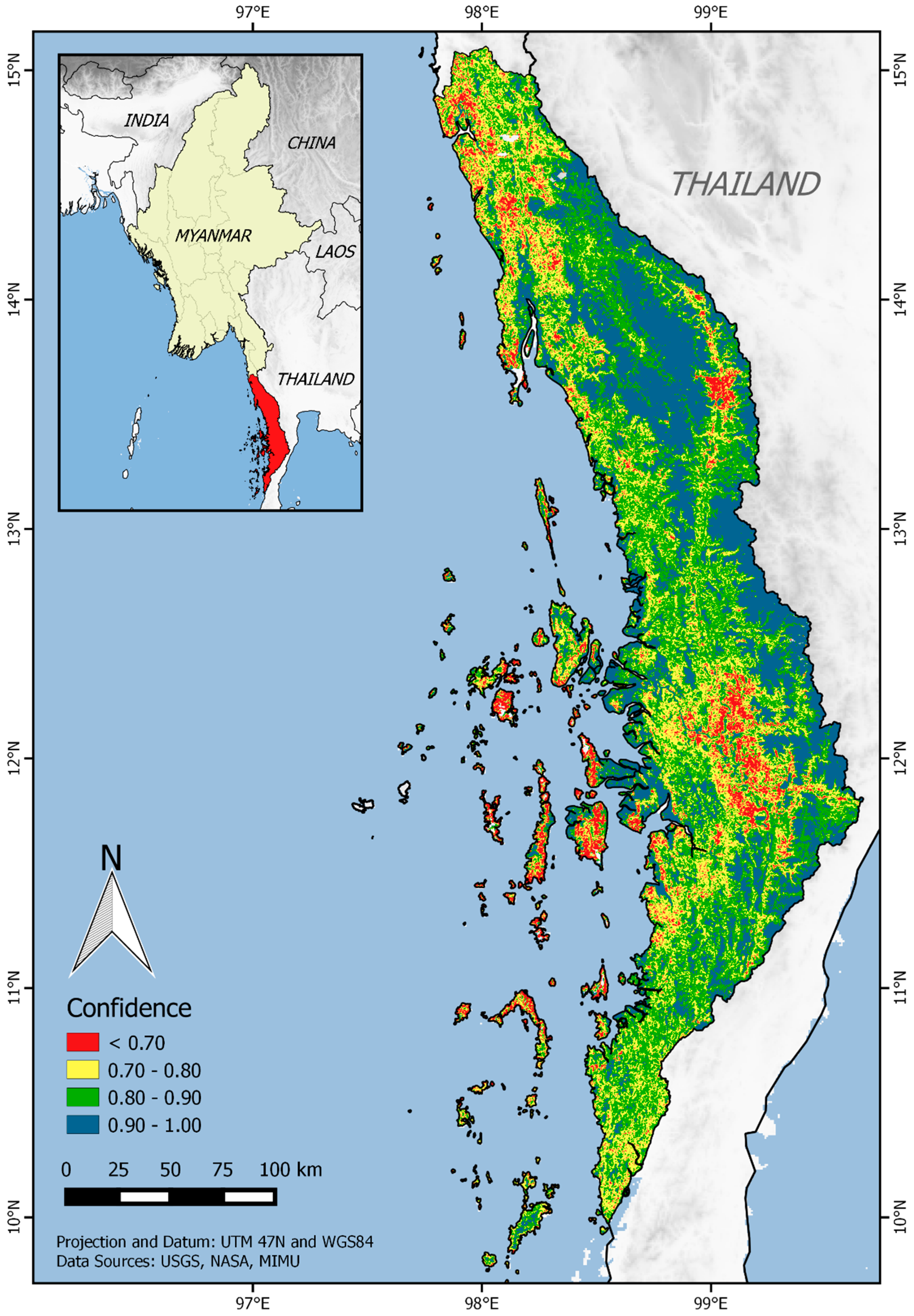
2.1. Study Area

Tanintharyi is the southernmost administrative region of Myanmar and covers over 43,000 km2 between the Andaman Sea to the west and Thailand to the east (Figure 1). Topography varies along this east–west gradient from flat or hilly coastal zones to mountainous areas of up to 2000 m in elevation along the Thai border. The region experiences a tropical monsoon climate with a distinct wet season, from May to October, followed by an extended dry season. Although forests in much of the region are broadleaf evergreen, certain areas contain mixtures or mosaics of evergreen and deciduous tree species. In monsoon areas of Southeast Asia, leaf drop occurs during the dry season for deciduous tree species, but can be highly variable among years, species, and locations [29,30]. For this study, we group forests in Tanintharyi into one of four major ecological types: (1) mangrove forest; (2) lowland evergreen forest; (3) upland evergreen forest; and (4) mixed deciduous forest.
In Tanintharyi, long-term conflict between the national government and various non-state armed groups previously resulted in a fragile security situation that limited the pace of development and forest loss [26,27]. As a result, the region retains extensive forests in the mountainous areas along the Thai border and has the largest remaining areas of biologically-rich lowland wet evergreen forest in the Sundaic region of continental Southeast Asia [6,27]. Concurrent with increased political stability, the landscape has been experiencing widespread deforestation [28] and rapid expansion of agriculture and agroforestry [26,31]. These land-use changes are focused primarily in low-elevation coastal areas, with remaining forest cover being increasingly concentrated in areas of steep terrain. Tanintharyi has a network of multi-use forest reserves as well as three protected areas, Lampi National Park, Moscos Islands Wildlife Sanctuary, and the Tanintharyi Nature Reserve. These areas cover 43.5% of the region, including extensive upland forests along the Thai border as well as island forests off the Tanintharyi coast.

2.2. Data and Preprocessing

We used Landsat 8 Operational Land Imager (OLI) data to map 16 land use and land cover classes for Tanintharyi, Myanmar (Table 1). We collected eight post-monsoon Landsat scenes with a narrow range of acquisition dates between 15 February and 18 March 2016 (Appendix A). We performed all image pre-processing and analysis steps using a series of scripts written for the R statistical software [32], which are available as Supplementary Materials. All Landsat data were first converted from Digital Numbers (DN) to Top of Atmosphere Reflectance (TOA) and Brightness Temperature (BT) values using radiometric rescaling coefficients from the Landsat metadata files [33]. We translated the FMASK algorithm [34,35] into R to perform image calibration, cloud removal and cloud shadow removal. We then used the C correction method [36] to conduct topographic normalization of Landsat 8 bands 2–7 (30-m resolution) using a 30-m resolution DEM to lessen the effects of topographic shadowing. Creation of training data for supervised land cover classification was dependent on the availability of free fine-resolution imagery (Google Earth or Bing Maps) and it was sometimes unknown which land cover types should occur in each Landsat scene. As a result, we ultimately created a single landscape-wide mosaic for each Landsat band after performing gamma correction (e.g., [37]) to reduce scene boundary artifacts by correcting for differences in overall luminance among scenes. Other data layers used in our analysis included a 30-m digital elevation model (DEM) from NASA’s Shuttle Radar Topography Mission [38], and a derived topographic position index (TPI) layer (e.g., [39]) in which the value of each cell represents the difference between the elevation of that cell and the mean elevation of all cells within the surrounding 1 km × 1 km neighborhood. The training data for our supervised land cover classification consisted of a 30-m resolution image stack containing each of the single-band mosaics for Landsat 8 bands 2–7 (blue, green, red, near-infrared, shortwave infrared 1, and shortwave infrared 2), as well as the DEM and TPI raster layers.

2.3. Mapping Approach

We used freely-available fine-resolution imagery (Google Earth or Bing Maps) to create training data polygons for supervised land cover classification. Satellite imagery available through these sources comes from a variety of data providers but is generally 65-cm resolution or finer and spans a range of image acquisition dates. Training data for this study were primarily based on imagery from 2014 to 2016, which was available for much of Tanintharyi. Visual interpretation of fine-resolution imagery was based on patch size and geometric shape, texture, color, or vegetation phenology in cases where time series of reference imagery were available. Although forest degradation can occur without a reduction of canopy cover, intact forest canopies in Tanintharyi are mostly closed [12]. As a result, we created training data for degraded forest classes in areas where early dry season canopy cover was less than 80%. Mixed deciduous forest was largely identified based on time series of imagery or prior knowledge of particular forest areas. Training data for lowland evergreen forest were created only in areas less than 200 m in elevation that were visually identified as having flat or gently undulating terrain. This process was done in consultation with field biologists knowledgeable about specific forest areas in Tanintharyi, and was also facilitated by field visits in March and May 2016. Training data polygons were manually digitized based on fine-resolution imagery and were subsequently reviewed using multiband composite rasters of pan-sharpened Landsat 8 imagery (15-m resolution). Each polygon was compared with both natural color (Landsat 8 bands 4-3-2) and color infrared (Landsat 8 bands 5-4-3) composite rasters to improve consistency between the training data and Landsat imagery. The final training dataset consisted of 75 polygons from each target land cover class.
We compared four separate land cover classifications to explore the effectiveness of mapping intact and degraded forest areas for specific forest types and the corresponding map accuracies. We conducted supervised classifications using both a Bayesian analysis of a multivariate Gaussian model and a Random Forest algorithm. These classifications were executed in R [32] using program JAGS [40,41] and the randomForest package [42], respectively. The multivariate Gaussian model is parametric classification procedure involving estimation of a mean vector and variance-covariance matrix based on spectral data from training samples, and is often referred to as the Gaussian Maximum Likelihood Classifier (e.g., [43]). Random Forest is a machine learning algorithm that is commonly used in remote sensing for classification of satellite or aerial images [44,45]. Random Forest is an ensemble decision tree classifier that is flexible with regards to distributional assumptions about the training data and is generally robust to over-fitting. As a result, this non-parametric classifier is potentially better suited to identification of target land cover classes that include mixtures of spectral information (see [44,45] for further details). For each classifier, we compared scenarios with just two natural forest classes (intact and degraded) to classifications with eight natural forest classes (intact and degraded for each of four distinct forest types). Each classified image was post-processed with a 3 × 3 majority filter to smooth isolated pixels that are likely to represent classification error.
The models were trained based on elevation, topographic position, and single-band Landsat data (for bands 2–7). These predictor variables were extracted from five randomly-selected pixels within each of the 50 training polygons for each land cover class, so that every target class was trained with 250 pixels. The remaining 25 training polygons for each class were withheld for an independent validation of map accuracy. For classifications with just two forest classes, we randomly selected 50 intact forest training polygons and 50 degraded forest polygons from the 200 available across all four ecological forest types. We also used output from the GMLC model to map pixel-level Bayesian posterior probabilities, which provide a measure of confidence that each pixel was assigned to the correct land use or land cover class in the analysis. To visualize broad-scale patterns of classification uncertainty, we resampled these pixel-level posterior probabilities to the mean for the surrounding 500 m × 500 m neighborhood (Figure 2). As further assessment of classification accuracy, we randomly selected one reference pixel from each of the 25 training polygons retained as validation data for each land cover class. Based on these points, we generated a confusion matrix to evaluate the accuracy of our class assignments for each combination of classifier (GMLC vs. Random Forest) and number of forest classes (two vs. eight). We summarize these results as per-class producer’s accuracies (fraction of reference pixels for a given class that are correctly identified), and per-class user’s accuracies (fraction of pixels of a given class that are correct in the classified image). Because training data were evenly split among classes, overall accuracy is equal to the mean per-class producer’s accuracy for each classification and is not reported separately. We also calculate the kappa coefficient for each classification, which represents an accuracy metric accounting for agreement due to chance [46]. Kappa coefficients are widely reported in remote sensing studies, though over-reliance on this metric has been criticized for, among other reasons, potentially overestimating chance agreement and the limited importance to map users of knowing whether accuracy is due to chance or design [47,48,49].

3. Results

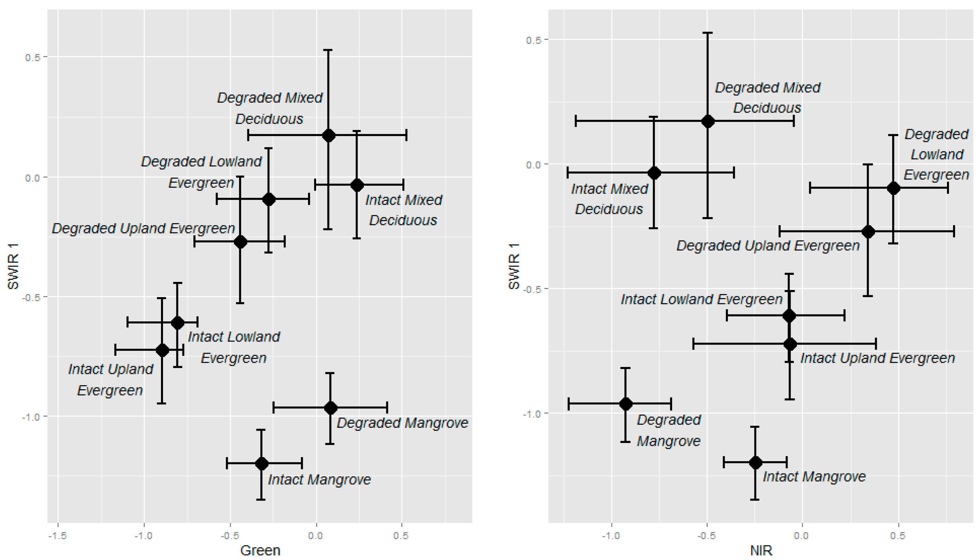
3.1. Mapping of Ecologically-Distinct Forest Types

For land cover classifications with just two natural forest classes (intact and degraded), validation based on withheld training data resulted in kappa coefficients of 0.70 and 0.78 for the GMLC and Random Forest classifications, respectively. The GMLC classifier had mean per-class user’s and producer’s accuracies of 74.2% and 73.2% Intact forest, degraded forest, and bare ground/clearing were frequently misclassified and had the three lowest user’s and producer’s accuracies by class. Overall, 28.0% of reference points for forest were misidentified as non-forest classes and an additional 16.0% were correctly identified as forest but incorrectly assigned as intact or degraded. The Random Forest classifier had mean per-class user’s and producer’s accuracies of 79.2% and 78.8%, respectively. User’s and producer’s accuracies were again low for the intact and degraded forest classes, with 24.0% of forest reference points being misclassified as non-forest classes versus 16.0% confusion of intact and degraded forest.
Partitioning forest cover into separate intact and degraded classes for each of four distinct forest types (mangrove, lowland evergreen, upland evergreen, and mixed deciduous) led to 3.3% and 3.6% increases in mean per-class user’s and producer’s accuracy based on the GMLC classification. The kappa coefficient for this classification improved from 0.70 to 0.75. Mean per-class producer’s accuracy for forest classes improved from 56% with just two forest classes to 72.5% with eight target forest classes. Furthermore, just 4.5% of reference points for forest were misidentified as a non-forest class, 8.5% were misclassified as a different forest type, and 14.5% were assigned the correct forest type but misidentified as intact or degraded. With the partitioning of intact and degraded forest into eight classes, there was a slight decrease in the kappa coefficient for the Random Forest classification, from 0.78 to 0.75. Mean per-class user’s and producer’s accuracies decreased by 1.9% and 2.0%, respectively. The forest type and intact or degraded status of reference points were correctly predicted 74.0% of the time. A further 6.0% of reference points for forest were misidentified as non-forest, 8.5% were misidentified as a different forest type, and 11.5% were assigned the correct forest type but misclassified as intact or degraded. Overall, the GMLC and Random Forest classifications with eight natural forest classes had the same kappa coefficients (0.75) and producer’s accuracies (76.8%), with the GMLC approach having a minimally higher mean per-class user’s accuracy (77.5% vs. 77.3%). All further results, tables, and figures reported are based on the GMLC classification due to the nearly-identical accuracy metrics and an apparent tendency to better predict land cover in several parts of the landscape where fine-resolution data were not available to create training data.

3.2. Extent of Remaining Forest Cover

Intact or degraded forest classes covered 80.7% of Tanintharyi, Myanmar in March 2016 (Figure 1 and Figure 3, Table 2). Upland evergreen forest was the most common forest type (42.3% of total area), followed by lowland evergreen forest (21.6%), mixed deciduous forest (10.8%), and mangrove forest (6.0%). The prevalence of forest degradation, or areas showing apparent canopy damage, varied widely among the four distinct forest types. Just 34.0% of mangrove forest was classified as intact (Figure 1B), compared to 47.1% of mixed deciduous forest, 52.5% of lowland evergreen forest, and 72.9% of remaining upland evergreen forest.
The major forest types in Tanintharyi also differ considerably in their representation within the national forest reserve and protected area systems. Combined, these government reserves encompass 56.2% of remaining intact forest. However, just 12.5% of intact mixed deciduous and 39.9% of intact mangrove forest fall within protected areas and forest reserves, compared to 60.8% and 62.7% of intact lowland and upland evergreen forest, respectively.

3.3. Human Land Use

We estimate that rice cultivation areas and mature oil palm, rubber, and betal nut plantations currently combine to cover 11.5% of Tanintharyi and 16.6% of all land outside protected areas and forest reserves. Rice cultivation covers 3.9% of the region, but is concentrated in flat, coastal areas. Commercial oil palm currently represents 3.4% of the landscape and primarily occurs in the Kawthaung district of southern Tanintharyi where extensive recent forest clearing suggests a continued expansion into some of the remaining tracts of lowland evergreen forest (Figure 1C). Mature rubber and betal nut plantations cover a further 2.2% and 2.1% of Tanintharyi, respectively. Areas of young agroforestry plantation without mature tree cover are believed to be primarily classified as clearing or degraded forest due to the dominant spectral signature of bare ground or early-successional vegetation. Given the rapid recent expansion of plantation areas and the large combined extents of bare ground and degraded forest classes, estimated plantation area in this study is likely highly conservative.

3.4. Accuracy Assessment

Training data for the eight natural forest classes encompassed a broad range of spectral variability (Figure 4). The overall per-class accuracies of the Tanintharyi land cover map ranged from 44% to 100% (Table 3). Of the error associated with natural forest classification, 52.7% of misclassified forest areas were due to confusion of canopy damaged areas and intact forest of the same forest type. Success distinguishing intact from degraded forest varied considerably among forest types, with degraded mixed deciduous forest being correctly identified just 44% of the time and most commonly confused with intact mixed deciduous. Areas of bare ground/clearing also had relatively low accuracy. New clearing is often a short-lived, transitional class and reference imagery may not always match the Landsat data used to perform the classification. Young plantation can also have spectral characteristics that are most similar to bare ground [50,51] or young regrowth in degraded forest areas. Finally, with the exception of rice cultivation areas, we observed a general tendency for predicted land cover in human-dominated parts of the landscape to have lower confidence (Figure 2). Many areas of Tanintharyi are composed of small plots of different land cover types, such as clearing, degraded forest, small-scale plantation, and areas of traditional shifting cultivation (i.e., slash-and-burn), and will often have a mixed spectral signature at 30-m resolution.

4. Discussion

4.1. Mapping of Forest Types and Degradation Extent

A key objective of this study was to effectively map forest degradation in Myanmar’s Tanintharyi Region in spite of spectral differences among forest types and varying levels of disturbance intensity across the landscape. This is a particular challenge in monsoon areas of Southeast Asia, where variation can be especially high among natural forest types in their physical structure and seasonal patterns of canopy cover [5]. Several studies have established that local floristic differences in tropical forest can be effectively mapped using medium-resolution multi-spectral imagery such as Landsat, typically in combination with topographic data [17,18,19,20,21]. However, increasing the variability within forest classes or the amount of spectral overlap between classes represents a considerable challenge to accurate discrimination of forest types [22]. This is a particular problem for studies that focus on mapping multiple unique forest types at geographic scales spanning multiple satellite images, having varying levels of topographic shadowing, or encompassing gradients in climate or forest disturbance [22].
In our study, forest areas spanned eight Landsat scenes that encompassed a considerable range of latitude, elevation, and climate conditions. In a comparison of GMLC and Random Forest classifications, we found that in either case there was just a slight increase (GMLC) or decrease (Random Forest) in overall classification accuracy by partitioning intact and degraded forest classes into separate classes for each of four ecological forest types. Because classification of remote sensing data primarily depends on the spectral contrast between classes, it is typically expected that increasing numbers of land cover classes will result in reduced classification accuracy [52]. Although the spectral difference between classes may be reduced with expanded classification schemes, inclusion of additional classes can also lead to increased spectral contrast by reducing the variability within individual classes. Parametric classifiers may especially likely to realize a net benefit from splitting classes with mixed spectral signatures into more homogeneous units, as indicated by the improvement in the accuracy of our GMLC classification by the addition of six additional forest classes. Most importantly, this expanded classification reduced the overall misidentification of forest reference points as non-forest from 28.0% to 4.5% and from 24.0% to 6.0% for the GMLC and Random Forest classifiers, respectively. Our study ultimately indicates that mapping of forest degradation can be more accurate with additional target classes representing distinct forest types, likely due to reduced variability within classes. However, we still found that identification of degraded areas within mixed deciduous forest had much lower accuracy than for other forest types.
A number of previous remote sensing studies have used multi-date satellite imagery to assess forest cover change dynamics in Myanmar. These include studies at global [53], national [6,12,24,54,55], and sub-national scales [14,23,55,56,57]. Countrywide studies have frequently focused on estimating overall rates of forest loss, without quantifying the unique threats faced by particular forest types (e.g., [6,12,24,58]). However, Wang and Myint [54] estimated nationwide deforestation rates (2001–2010) for each of five unique forest types and found that mangrove and deciduous forest had experienced deforestation rates that were 2–5 times the national average. Bhagwat et al. [12] did not distinguish specific forest types, but provided rates of deforestation, forest degradation, and conversion to agroforestry plantations. Forest loss data from Hansen et al. [53] have also been previously used to highlight the loss of lowland evergreen forest in Tanintharyi, Myanmar [27]. Although our study represents a single-date land cover map for Tanintharyi, this detailed classification provides insight into the local drivers of forest loss identified in previous studies. For instance, 42% of forest gain (2002–2014) according to Hansen et al. [53] was identified as agroforestry plantation in our 2016 land cover (oil palm, rubber, betal nut) and a further 38% was assigned to a degraded forest class. Just 6% of areas classified as deforested from 2002 to 2014 were classified as intact forest in our dataset. Conversely, less than 1% of intact forest pixels in our dataset were deforested between 2002 and 2014 according to Hansen et al. [53], suggesting a general agreement between the two datasets.

4.2. Current Status of Tanintharyi’s Major Forest Ecosystems

We found that Myanmar’s Tanintharyi region remains predominantly forested, with large contiguous expanses of upland evergreen and mixed deciduous forest in the Dawna and Tenasserim Mountains along the Myanmar-Thai border. Although these large forested areas were still primarily intact, expanded forest degradation and plantation development were apparent along several road corridors connecting Myanmar and Thailand that may threaten wildlife habitat connectivity. Such road developments may also be a precursor to deforestation because they increase access and reduce the perceived conservation value of an area [59].
Our study also highlights the limited extent of remaining intact lowland evergreen forest and the highly-degraded nature of Tanintharyi’s mangroves. Forests in lowland or coastal areas have experienced especially high rates of forest loss throughout Southeast Asia due to their greater accessibility and proximity to areas of higher human population density [6,7,27]. Mangrove forests are found in the inter-tidal zone in tropical and sub-tropical areas, harboring unique biodiversity while providing significant ecosystem services such as coastal protection, erosion control, enhanced fisheries, carbon sequestration and fuel wood [60]. However, mangroves are one of the least protected habitat types in Myanmar [28] and the country has the highest rate of mangrove loss in Southeast Asia [8]. Recent estimates for nationwide mangrove deforestation rates vary considerably, but indicate that mangrove loss is occurring much more rapidly than loss of other forest types [8,54]. In the current study, we estimated the total mangrove area in Tanintharyi as 2430 km2, with 66.0% of remaining mangrove extent being in degraded condition (Table 2).
We also found that the current distribution of intact lowland evergreen forest covers just 11.4% of Tanintharyi while oil palm cultivation continues to replace and fragment many remaining areas. In spite of the low predicted yields for oil palm in Tanintharyi [27,61], large-scale concessions awarded for oil palm plantations totaled 1.9 million acres by 2013 [26]. There have also been reports that oil palm development has been motivated or reinforced by logging interests (e.g., [26]), and our land cover classification indicates that extensive patches of lowland forest have been cleared in areas where oil palm has only been successfully established along narrow roadside strips (Figure 1C). A recent study estimated that 23% of total land area in Tanintharyi is now agroforestry plantation [31]. Although this total differs considerably from the total areas of mature oil palm, rubber, and betal nut cultivation reported in our study (11.5%), we identified a further 3.9% of the landscape as recent clearing and 30% as degraded forest, which may include young plantation with early-successional vegetation. These rapid changes occurring in Tanintharyi highlight the urgent need for accurate land use data and rigorous spatial planning to support conservation efforts.

5. Conclusions

Our study was conducted with the overall goal of mapping forest extent and identifying areas of forest degradation across a number of structurally- and ecologically-distinct forest types in Tanintharyi, Myanmar. We found that discrimination among forest types was possible with little or no loss of overall classification accuracy while greatly increasing the relevance of the map for purposes of conservation and land use planning. Furthermore, we provide current land use data for a rapidly-developing region of Myanmar that is home to some of the country’s largest remaining areas of intact forest. The Myanmar government has a target of formally designating 10% of the country’s area for its Protected Area System [28]. Mangrove and lowland evergreen forests represent globally-significant ecosystems, yet both are currently under-represented in the country’s Protected Area System [28]. Our study highlights the threats faced by these unique forest types as a result of rapid development and surrounding land use conversion.

Supplementary Materials

The following are available online at www.mdpi.com/2072-4292/8/11/882/s1. Supplementary materials include R code for Landsat pre-processing and GMLC classification methods described in the manuscript.

Acknowledgments

We thank our editors and several anonymous reviewers for constructive feedback on this manuscript. We are also grateful to Saw Htun, Kyaw Thinn Latt, and Robert Tizard (Wildlife Conservation Society), as well as Frank Momberg and Mark Grindley (Fauna & Flora International) for their comments and insight on this project. We also thank Nyi Nyi Kyaw and Soe Thiha of the Myanmar Forest Department for facilitating field data collection and providing their expert input. We thank Ko Zaw Myo, Ko Hein, Ko Khin Zaw Moe, Ko Aung Myint, Ko Tu Tu and Saw War Mei Sai for assistance with field visits to the Tanintharyi Nature Reserve. Funding for this research was provided by The Leona M. and Harry B. Helmsley Charitable Trust.

Author Contributions

Grant Connette conceived and designed the study, developed code for data processing and analysis, and wrote the paper. Patrick Oswald advised on the methodology, contributed ideas for the manuscript, and provided comments on a draft manuscript. Melissa Songer and Peter Leimgruber assisted in conceiving the study, advised on methodology, and provided revisions to the manuscript.

Conflicts of Interest

The authors declare no conflict of interest.

Appendix A

Table A1. Landsat scenes and tiles used in the analysis.
Landsat Scene Details
Tile DateLandsat 8 Identifier
129_5211 March 2016LC81290522016071
130_5015 February 2016LC81300502016046
130_5115 February 2016LC81300512016046
130_5218 March 2016LC81300522016078
130_5318 March 2016LC81300532016078
131_509 March 2016LC81310502016069
131_519 March 2016LC81310512016069
131_529 March 2016LC81310522016069

References

  1. De Bruyn, M.; Stelbrink, B.; Morley, R.J.; Hall, R.; Carvalho, G.R.; Cannon, C.H.; van den Bergh, G.; Meijaard, E.; Metcalfe, I.; Boitani, L.; et al. Borneo and Indochina are major evolutionary hotspots for Southeast Asian biodiversity. Syst. Biol. 2014, 63, 879–901. [Google Scholar] [CrossRef] [PubMed]
  2. Myers, N.; Mittermeier, R.A.; Mittermeier, C.G.; da Fonseca, G.A.B.; Kent, J. Biodiversity hotspots for conservation priorities. Nature 2000, 403, 853–858. [Google Scholar] [CrossRef] [PubMed]
  3. Wohlfart, C.; Wegmann, M.; Leimgruber, P. Mapping threatened dry deciduous dipterocarp forest in South-east Asia for conservation management. Trop. Conserv. Sci. 2014, 7, 597–613. [Google Scholar] [CrossRef]
  4. Wijedasa, L.S.; Sloan, S.; Michelakis, D.G.; Clements, G.R. Overcoming limitations with Landsat imagery for mapping of peat swamp forests in Sundaland. Remote Sens. 2012, 4, 2595–2618. [Google Scholar] [CrossRef]
  5. Miettinen, J.; Stibig, H.-J.; Achard, F. Remote sensing of forest degradation in Southeast Asia—Aiming for a regional view through 5–30 m satellite data. Glob. Ecol. Conserv. 2014, 2, 24–36. [Google Scholar] [CrossRef]
  6. Leimgruber, P.; Kelly, D.S.; Steininger, M.K.; Brunner, J.; Müller, T.; Songer, M. Forest cover change patterns in Myanmar (Burma) 1990–2000. Environ. Conserv. 2005, 32, 356–364. [Google Scholar] [CrossRef]
  7. Stibig, H.-J.; Stolle, F.; Dennis, R.; Feldkötter, C. Forest Cover Change in Southeast Asia. The Regional Pattern; European Commission Joint Research Centre: Ispra, Italy, 2007. [Google Scholar]
  8. Richards, D.R.; Friess, D.A. Rates and drivers of mangrove deforestation in Southeast Asia, 2000–2012. Proc. Natl. Acad. Sci. USA 2016, 113, 344–349. [Google Scholar] [CrossRef] [PubMed]
  9. Ryan, C.M.; Hill, T.; Woollen, E.; Ghee, C.; Mitchard, E.; Cassells, G.; Grace, J.; Woodhouse, I.H.; Williams, M. Quantifying small-scale deforestation and forest degradation in African woodlands using radar imagery. Glob. Chang. Biol. 2012, 18, 243–257. [Google Scholar] [CrossRef]
  10. Ahrends, A.; Burgess, N.D.; Milledge, S.A.H.; Bulling, M.T.; Fisher, B.; Smart, J.C.R.; Clarke, G.P.; Mhoro, B.E.; Lewis, S.L. Predictable waves of sequential forest degradation and biodiversity loss spreading from an African city. Proc. Natl. Acad. Sci. USA 2010, 107, 14556–14561. [Google Scholar] [CrossRef] [PubMed]
  11. Matricardi, E.A.T.; Skole, D.L.; Cochrane, M.A.; Pedlowski, M.; Chomentowski, W. Multi-temporal assessment of selective logging in the Brazilian Amazon using Landsat data. Int. J. Remote Sens. 2007, 28, 63–82. [Google Scholar] [CrossRef]
  12. Bhagwat, T.; Hess, A.; Horning, N.; Khaing, T.; Thein, Z.M.; Aung, K.M.; Aung, K.H.; Phyo, P.; Tun, Y.L.; Oo, A.H.; et al. Losing a jewel—Rapid declines in Myanmar’s intact forests from 2002–2014. PLoS ONE 2016. in review. [Google Scholar]
  13. Souza, C.M., Jr.; Roberts, D.A.; Cochrane, M.A. Combining spectral and spatial information to map canopy damage from selective logging and forest fires. Remote Sens. Environ. 2005, 98, 329–343. [Google Scholar] [CrossRef]
  14. Mon, M.S.; Mizoue, N.; Htun, N.Z.; Kajisa, T.; Yoshida, S. Factors affecting deforestation and forest degradation in selectively logged production forest: A case study in Myanmar. For. Ecol. Manag. 2012, 267, 190–198. [Google Scholar] [CrossRef]
  15. Souza, C.M., Jr.; Barreto, P. An alternative approach for detecting and monitoring selectively logged forests in the Amazon. Int. J. Remote Sens. 2000, 21, 173–179. [Google Scholar] [CrossRef]
  16. Suepa, T.; Qi, J.; Lawawirojwong, S.; Messina, J.P. Understanding spatio-temporal variation of vegetation phenology and rainfall seasonality in the monsoon Southeast Asia. Environ. Res. 2016, 147, 621–629. [Google Scholar] [CrossRef] [PubMed]
  17. Thessler, S.; Sesnie, S.; Ramos Bendaña, Z.S.; Ruokolainen, K.; Tomppo, E.; Finegan, B. Using k-nn and discriminant analyses to classify rain forest types in a Landsat TM image over northern Costa Rica. Remote Sens. Environ. 2008, 112, 2485–2494. [Google Scholar] [CrossRef]
  18. Sesnie, S.E.; Finegan, B.; Gessler, P.E.; Thessler, S.; Bendana, Z.R.; Smith, A.M.S. The multispectral separability of Costa Rican rainforest types with support vector machines and random forest decision trees. Int. J. Remote Sens. 2010, 31, 2885–2909. [Google Scholar] [CrossRef]
  19. Salovaara, K.J.; Thessler, S.; Malik, R.N.; Tuomisto, H. Classification of Amazonian primary rain forest vegetation using Landsat ETM+ satellite imagery. Remote Sens. Environ. 2005, 97, 39–51. [Google Scholar] [CrossRef]
  20. Fagan, M.E.; DeFries, R.S.; Sesnie, S.E.; Arroyo-Mora, J.P.; Soto, C.; Singh, A.; Townsend, P.A.; Chazdon, R.L. Mapping species composition of forests and tree plantations in northeastern Costa Rica with an integration of hyperspectral and multitemporal Landsat imagery. Remote Sens. 2015, 7, 5660–5696. [Google Scholar] [CrossRef]
  21. Foody, G.M.; Cutler, M.E.J. Tree biodiversity in protected and logged Bornean tropical rain forests and its measurement by satellite remote sensing. J. Biogeogr. 2003, 30, 1053–1066. [Google Scholar] [CrossRef]
  22. Helmer, E.H.; Goodwin, N.R.; Gond, V.; Souza, C.M., Jr.; Asner, G.P. Characterizing tropical forests with multispectral imagery. In Land Resources: Monitoring, Modeling and Mapping; Thenkabail, P.S., Ed.; CRC Press: Boca Raton, FL, USA, 2015. [Google Scholar]
  23. Webb, E.L.; Jachowski, N.R.A.; Phelps, J.; Friess, D.A.; Than, M.M.; Ziegler, A.D. Deforestation in the Ayeyarwady delta and the conservation implications of an internationally-engaged Myanmar. Glob. Environ. Chang. 2014, 24, 321–333. [Google Scholar] [CrossRef]
  24. Food and Agriculture Organization of the United Nations (FAO). Global Forest Resources Assessment; FAO: Rome, Italy, 2015. [Google Scholar]
  25. Woods, K. Timber Trade Flows and Actors in Myanmar: The Political Economy of Myanmar’s Timber Trade; Forest Trends: Washington, DC, USA, 2013. [Google Scholar]
  26. Woods, K. Commercial Agriculture Expansion in Myanmar: Links to Deforestation, Conversion Timber, and Land Conflicts; Forest Trends: Washington, DC, USA, 2015. [Google Scholar]
  27. Donald, P.F.; Round, P.D.; Aung, T.D.W.; Grindley, M.; Steinmetz, R.; Shwe, N.M.; Buchanan, G.M. Social reform and a growing crisis for southern Myanmar’s unique forests. Conserv. Biol. 2015, 29, 1485–1488. [Google Scholar] [CrossRef] [PubMed]
  28. Ministry of Environmental Conservation and Forestry (MOECAF). The Republic of the Union of Myanmar: National Biodiversity Strategy and Action Plan; Ministry of Environmental Conservation and Forestry (MOECAF): Naypyidaw, Myanmar, 2011.
  29. Williams, L.J.; Bunyavejchewin, S.; Baker, P.J. Deciduousness in a seasonal tropical forest in western Thailand: Interannual and intraspecific variation in timing, duration and environmental cues. Oecologia 2008, 155, 571–582. [Google Scholar] [CrossRef] [PubMed]
  30. Elliott, S.; Baker, P.J.; Borchert, R. Leaf flushing during the dry season: The paradox of Asian monsoon forests. Glob. Ecol. Biogeogr. 2006, 15, 248–257. [Google Scholar] [CrossRef]
  31. Torbick, N.; Ledoux, L.; Salas, W.; Zhao, M. Regional mapping of plantation extent using multisensor imagery. Remote Sens. 2016, 8. [Google Scholar] [CrossRef]
  32. R Core Team. R: A language and Environment for Statistical Computing; R Foundation for Statistical Computing: Vienna, Austria, 2014. [Google Scholar]
  33. Chander, G.; Markham, B.L.; Helder, D.L. Summary of current radiometric calibration coefficients for Landsat MSS, TM, ETM+, and EO-1 ALI sensors. Remote Sens. Environ. 2009, 113, 893–903. [Google Scholar] [CrossRef]
  34. Zhu, Z.; Wang, S.; Woodcock, C.E. Improvement and expansion of the fmask algorithm: Cloud, cloud shadow, and snow detection for Landsats 4–7, 8, and Sentinel 2 images. Remote Sens. Environ. 2015, 159, 269–277. [Google Scholar] [CrossRef]
  35. Zhu, Z.; Woodcock, C.E. Object-based cloud and cloud shadow detection in Landsat imagery. Remote Sens. Environ. 2012, 118, 83–94. [Google Scholar] [CrossRef]
  36. Riano, D.; Chuvieco, E.; Salas, J.; Aguado, I. Assessment of different topographic corrections in Landsat-TM data for mapping vegetation types (2003). IEEE Trans. Geosci. Remote Sens. 2003, 41, 1056–1061. [Google Scholar] [CrossRef]
  37. Hunt, R.W.G. The Reproduction of Colour, 6th ed.; John Wiley & Sons: Chichester, West Sussex, UK, 2005. [Google Scholar]
  38. Farr, T.G.; Rosen, P.A.; Caro, E.; Crippen, R.; Duren, R.; Hensley, S.; Kobrick, M.; Paller, M.; Rodriguez, E.; Roth, L.; et al. The shuttle radar topography mission. Rev. Geophys. 2007, 45, RG2004. [Google Scholar] [CrossRef]
  39. Guisan, A.; Weiss, S.B.; Weiss, A.D. GLM versus CCA spatial modeling of plant species distribution. Plant Ecol. 1999, 143, 107–122. [Google Scholar] [CrossRef]
  40. Plummer, M. Jags: A Program for Analysis of Bayesian Graphical Models Using Gibbs Sampling. 2003. Available online: http://citeseer.ist.psu.edu/plummer03jags.html (accessed on 18 August 2015).
  41. Kellner, K. Jagsui: A Wrapper around ‘Rjags’ to Streamline ‘Jags’ Analyses. Available online: http://CRAN.R-project.org/package=jagsUI (accessed on 7 September 2015).
  42. Liaw, A.; Wiener, M. Classification and regression by randomforest. R News 2002, 2, 18–22. [Google Scholar]
  43. Lillesand, T.; Kiefer, R.W.; Chipman, J. Remote Sensing and Image Interpretation; John Wiley & Sons: New York, NY, USA, 2014. [Google Scholar]
  44. Horning, N. Random forests: An algorithm for image classification and generation of continuous fields data sets. In Proceedings of the International Conference on Geoinformatics for Spatial Infrastructure Development in Earth and Allied Sciences, Osaka, Japan, 9–11 December 2010.
  45. Rodriguez-Galiano, V.F.; Ghimire, B.; Rogan, J.; Chica-Olmo, M.; Rigol-Sanchez, J.P. An assessment of the effectiveness of a random forest classifier for land-cover classification. ISPRS J. Photogramm. Remote Sens. 2012, 67, 93–104. [Google Scholar] [CrossRef]
  46. Cohen, J. Weighted kappa: Nominal scale agreement provision for scaled disagreement or partial credit. Psychol. Bull. 1968, 70, 213–220. [Google Scholar] [CrossRef] [PubMed]
  47. Foody, G.M. On the compensation for chance agreement in image classification accuracy assessment. Photogramm. Eng. Remote Sens. 1992, 58, 1459–1460. [Google Scholar]
  48. Foody, G.M. Harshness in image classification accuracy assessment. Int. J. Remote Sens. 2008, 29, 3137–3158. [Google Scholar] [CrossRef]
  49. Nishii, R.; Tanaka, S. Accuracy and inaccuracy assessments in land-cover classification. IEEE Trans. Geosci. Remote Sens. 1999, 37, 491–498. [Google Scholar] [CrossRef]
  50. Dong, J.; Xiao, X.; Chen, B.; Torbick, N.; Jin, C.; Zhang, G.; Biradar, C. Mapping deciduous rubber plantations through integration of PALSAR and multi-temporal Landsat imagery. Remote Sens. Environ. 2013, 134, 392–402. [Google Scholar] [CrossRef]
  51. Li, Z.; Fox, J.M. Mapping rubber tree growth in mainland Southeast Asia using time-series MODIS 250 m NDVI and statistical data. Appl. Geogr. 2012, 32, 420–432. [Google Scholar] [CrossRef]
  52. Bhatta, B. Research Methods in Remote Sensing; Springer: Dordrecht, the Netherlands, 2013. [Google Scholar]
  53. Hansen, M.C.; Potapov, P.V.; Moore, R.; Hancher, M.; Turubanova, S.A.; TyUKavina, A.; Thau, D.; Stehman, S.V.; Goetz, S.J.; Loveland, T.R.; et al. High-resolution global maps of 21st-century forest cover change. Science 2013, 342, 850–853. [Google Scholar] [CrossRef] [PubMed]
  54. Wang, C.; Myint, S. Environmental concerns of deforestation in Myanmar 2001–2010. Remote Sens. 2016. [Google Scholar] [CrossRef]
  55. Songer, M.; Myint, A.; Senior, B.; Defries, R.; Leimgruber, P. Spatial and temporal deforestation dynamics in protected and unprotected dry forests: A case study from Myanmar (Burma). Biodivers. Conserv. 2009, 18, 1001–1018. [Google Scholar] [CrossRef]
  56. Htun, N.Z.; Mizoue, N.; Kajisa, T.; Yoshida, S. Deforestation and forest degradation as measures of popa mountain park (Myanmar) effectiveness. Environ. Conserv. 2009, 36, 218–224. [Google Scholar] [CrossRef]
  57. Renner, S.C.; Rappole, J.H.; Leimgruber, P.; Kelly, D.S.; Shwe, N.M.; Aung, T.; Aung, M. Land cover in the northern forest complex of Myanmar: New insights for conservation. Oryx 2007, 41, 27–37. [Google Scholar] [CrossRef]
  58. Liu, F.-J.; Huang, C.; Pang, Y.; Li, M.; Song, D.-X.; Song, X.-P.; Channan, S.; Sexton, J.O.; Jiang, D.; Zhang, P.; et al. Assessment of the three factors affecting Myanmar’s forest cover change using Landsat and MODIS vegetation continuous fields data. Int. J. Digit. Earth 2016, 9, 562–585. [Google Scholar] [CrossRef]
  59. Asner, G.P.; Broadbent, E.N.; Oliveira, P.J.; Keller, M.; Knapp, D.E.; Silva, J.N. Condition and fate of logged forests in the Brazilian amazon. Proc. Natl. Acad. Sci. USA 2006, 103, 12947–12950. [Google Scholar] [CrossRef] [PubMed]
  60. Barbier, E.B.; Hacker, S.D.; Kennedy, C.; Koch, E.W.; Stier, A.C.; Silliman, B.R. The value of estuarine and coastal ecosystem services. Ecol. Monogr. 2011, 81, 169–193. [Google Scholar] [CrossRef]
  61. Baskett, J.P.C. Myanmar oil Palm Plantations: A Productivity and Sustainability Review; Fauna & Flora International: Yangon, Myanmar, 2015. [Google Scholar]
Figure 1. Land cover classification for Myanmar’s Tanintharyi Region in 2016 (A); Mangrove degradation south of the city of Myeik (B); Oil palm plantation development and lowland evergreen forest in Tanintharyi’s Kawtaung District (C).
Remotesensing 08 00882 g001
Figure 2. Map of Bayesian posterior probabilities for the land cover classification of Tanintharyi Region, Myanmar. High values indicate locations for which model-based assignment to a land cover class had high certainty. All pixel values are resampled to represent the mean posterior probability for each 500 m × 500 m neighborhood.
Remotesensing 08 00882 g002
Figure 3. Combined extents of intact forest, degraded forest, and non-forest classes for Myanmar’s Tanintharyi Region.
Remotesensing 08 00882 g003
Figure 4. Normalized Top of Atmosphere Reflectance (TOA) of training data by forest type. Points indicate mean values while error bars depict upper and lower quartiles for Landsat 8 bands 3 (green), 5 (near infrared), and 6 (shortwave infrared 1). For each band, normalized reflectance was calculated by subtracting the mean and dividing by the standard deviation of the training data sample.
Remotesensing 08 00882 g004
Table 1. Tanintharyi land use and land cover categories.
CategoryDescription
Intact Upland Evergreen ForestCanopy cover ≥80%. Elevation >200 m or on steep terrain at lower elevations. Canopy remains green year round.
Degraded Upland Evergreen ForestCanopy cover <80%. Elevation >200 m or on steep terrain at lower elevations. Canopy remains green year round.
Intact Lowland Evergreen ForestCanopy cover ≥80%. Elevation <200 m or on flat or level terrain. Canopy remains green year round.
Degraded Lowland Evergreen ForestCanopy cover <80%. Elevation <200 m or on flat or level terrain. Canopy remains green year round.
Intact Mangrove ForestMangrove cover ≥80%.
Degraded Mangrove ForestMangrove cover <80%. Evidence of thinning visible as bare ground from above.
Intact Mixed Deciduous ForestCanopy cover ≥80%. Mixture of trees with and without leaves during dry season.
Degraded Mixed Deciduous ForestCanopy cover ≥80%. Mixture of trees with and without leaves during dry season.
Oil Palm PlantationMature oil palm. Oil palm coverage >50%.
Rubber PlantationMature rubber plantation. Rubber coverage >50%.
Betal Nut Garden/PlantationMature betal nut garden, plantation, or planting in forest
SettlementAreas with interspersed to complete coverage of buildings and man-made structures.
RiceRice
MudflatCoastal and estuarine mudflats
Bare Ground/ClearingExposed soil and recent clearings with grassy or low herbaceous vegetation cover
WaterOcean, rivers, lakes, reservoirs, flooded areas.
Table 2. Terrestrial land cover by area in Tanintharyi, Myanmar.
Land CoverArea (km2)Percent of Total
Degraded Mangrove16044.0
Intact Mangrove8262.1
Degraded Lowland Evergreen414110.4
Intact Lowland Evergreen458011.5
Degraded Upland Evergreen462411.6
Intact Upland Evergreen12,45631.2
Degraded Mixed Deciduous22955.8
Intact Mixed Deciduous20465.1
Bare Ground/Clearing15293.8
Rice15423.9
Oil Palm Plantation13653.4
Rubber Plantation12752.1
Betal Nut Garden/Plantation8212.2
Settlement8663.0
Total39,897100.0
Table 3. Confusion matrix from the Gaussian Maximum Likelihood Classification (GMLC) for 16 land use/land cover classes. Numbers of correctly classified reference points (withheld training data) are shown in bold along the main diagonal. Land use/land cover codes are: wa, water; dv, degraded mangrove; iv, intact mangrove; dl, degraded lowland evergreen forest; il, intact lowland evergreen forest; du, degraded upland evergreen forest; iu, intact upland evergreen forest; dm, degraded mixed deciduous forest; im, intact mixed deciduous forest; cl, clearing/bare ground; ri, rice; oi, oil palm; ru, rubber; be, betal nut; mu, mudflat; se, human settlement.
Reference Points
wadvivdlilduiudmimclrioirubemuse
wa25000000000000000
dv02240000000100000
iv01210000000000000
dl00018110122000200
il00032011100000000
du00001141210000000
iu00002423100000000
dm00000101164010200
im00000209161000000
cl00000000013000003
ri01000000022100033
oi01011000000222200
ru00010000001022000
be00010200002001800
mu00000000000000220
se00010000030211019
Producer’s Accuracies:
1.000.880.840.720.800.560.920.440.640.520.840.880.880.720.880.76
User’s Accuracies:
1.000.810.950.670.770.740.770.440.570.810.700.760.920.781.000.70

