
Manifold Learning Co-Location Decision Tree for Remotely Sensed Imagery Classification

Abstract
:
1. Introduction
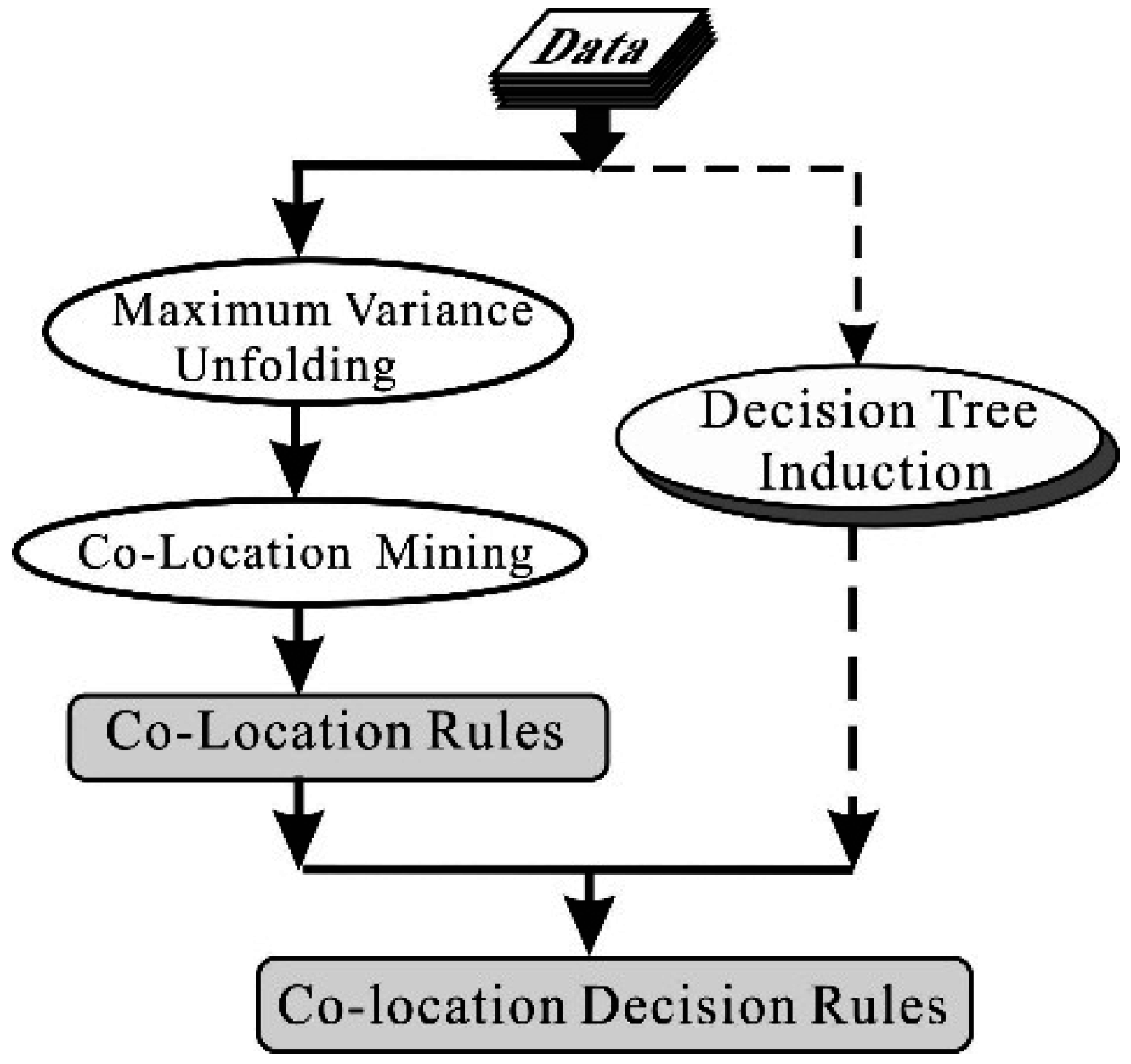
2. MVU-Based Co-Location Decision Tree Induction Method
2.1. Brief Review of MVU
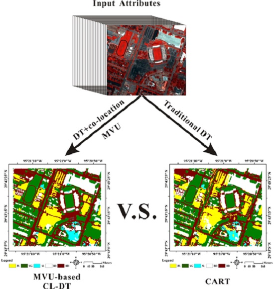
2.2. Basic Idea of the Proposed MVU-Based CL-DT
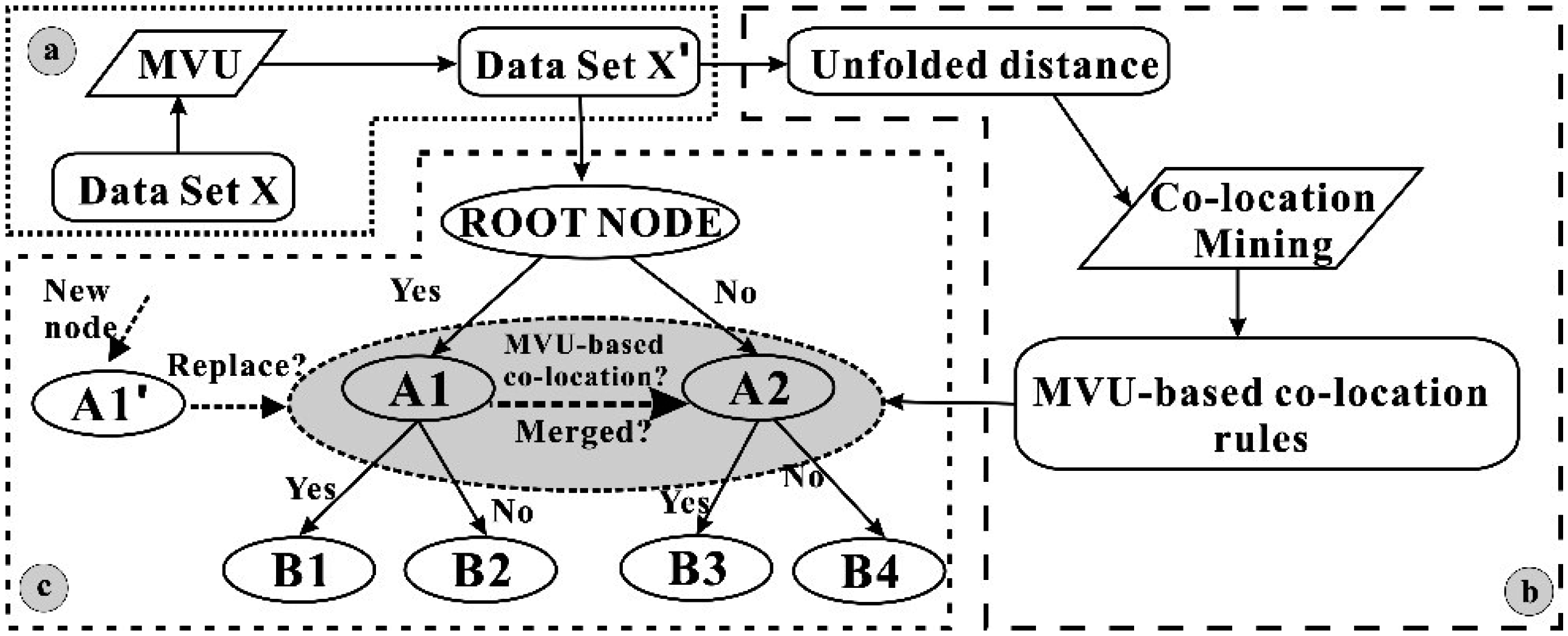
- Unfold the input data using the MVU method. To obtain the unfolded distance between instances, the original input dataset X, which is a nonlinear distribution in higher-dimensional space, is preprocessed using the MVU method. A new dataset X′, which is regarded as a linear distribution, is obtained and employed to: (1) calculate the unfolded distance; and (2) become the root node of the DT.
- Mine co-location rules. Co-location rules are mined through a co-location algorithm with the unfolded distances, which are calculated from the dataset X′.
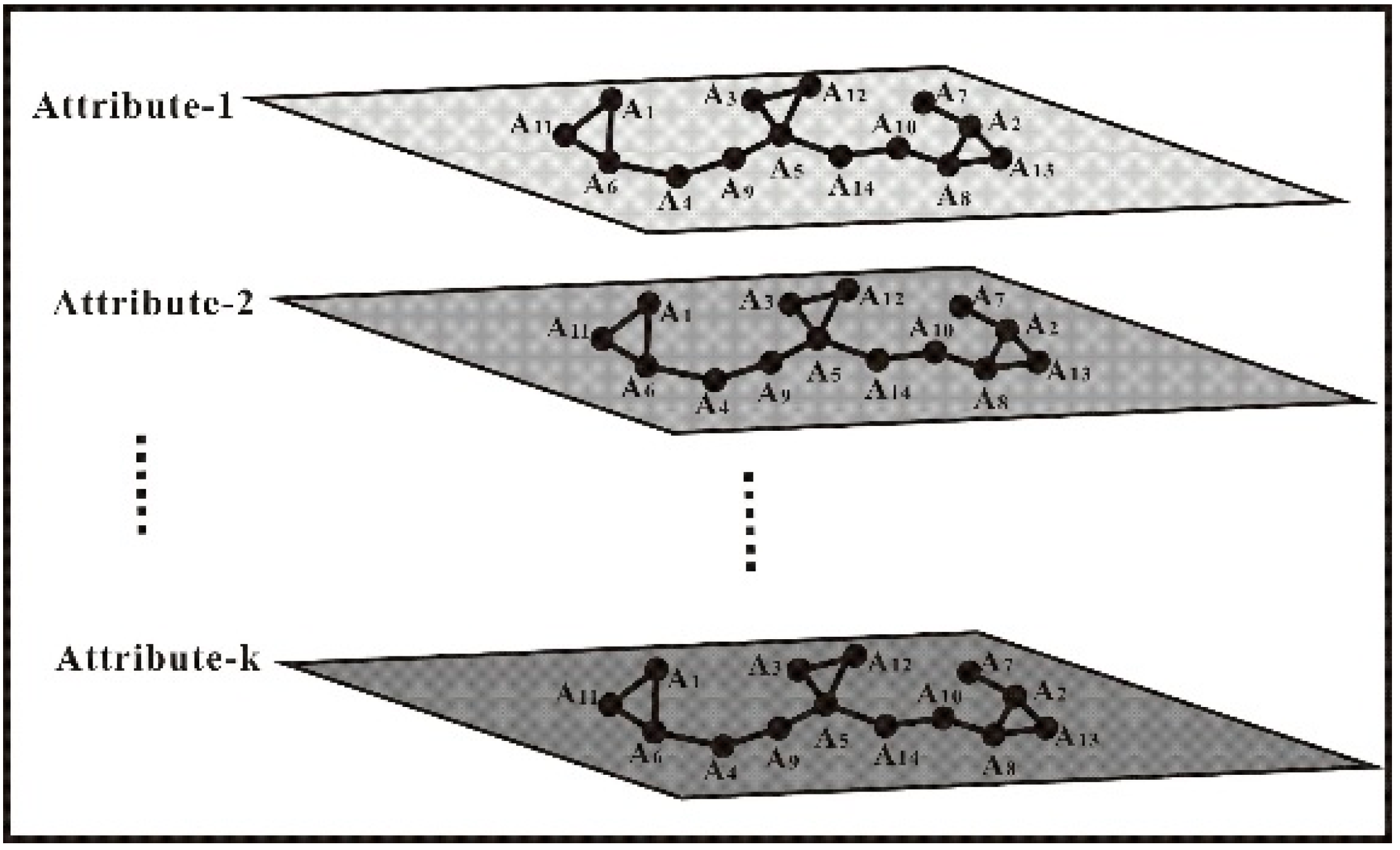
- Generate MVU-based CL-DT. The dataset X′ is taken as the input data of the root node of the DT. At the beginning, all attributes of dataset X′ are “accepted” by the root node, and one “best” attribute, such as BA1, is selected from the input dataset X′; then, a splitting criterion is used to determine whether the root node will be split using a binary decision (Yes or No in Figure 2) into two intermediate nodes, noted by wi and wj (w = A, i = 1, and j = 2 in Figure 2). For each of the intermediate nodes (wi and wj), the splitting criterion will be applied to determine whether the node should be further split. If No, this node is considered a leaf node, and one of the class labels is assigned to this leaf node. If Yes, this node will be split by selecting another “best” attribute, BA2. Meanwhile, the MVU-based co-location criterion will be used to judge whether the “best” attribute BA2 is co-located with BA1 at the same layer. If Yes, this node will be “merged” into the node and named a co-location node. For example, nodes A1 and A2 are merged into a new node A1′ in Figure 2. After that, one new “best” attribute will again be selected, and whether the selected “best” attribute co-occurs with the last “best” attribute is re-judged. If No, the node will be further split into a sub-set by repeating the above operation. These above processes are repeated until all data have been processed.
2.3. MVU-Based Co-Location Mining Rules
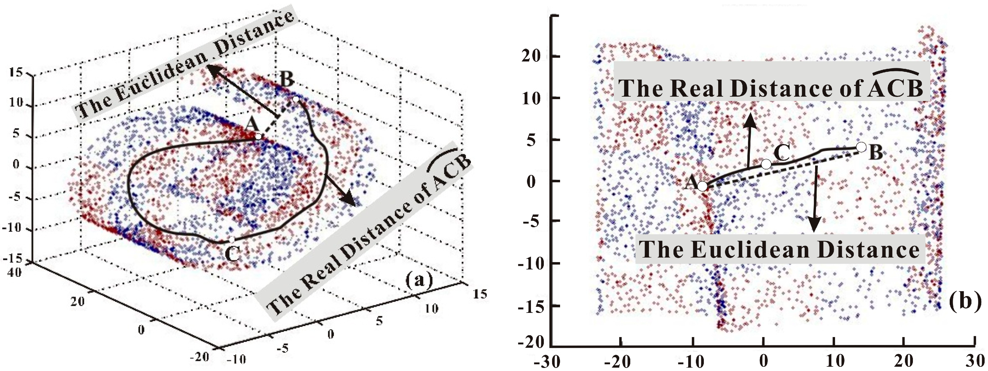
2.3.1. MVU Unfolded Distance Algorithm
| Algorithm 1. The Algorithm of MUD |
| 1. Input: The number of nearest neighbors k; Original data set X; An N × N zero matrix |
| 2. Output: Low-dimensional representation Y; An N × N binary matrix ; An Unfolded distance matrix U |
| 3. Process: |
| 4. Step 1: Construct the neighbor graph. |
| 5. If Xi and Xk satisfy K-NN Then ; else ; |
| 6. Step 2: Semidefinite programming. |
| 7. Compute the maximum variance unfolding Gram matrix L of sample pairwise points, which is centered on the origin. |
| 8. Max{tr(L)} s.t. L ≥ 0, and . |
| 9. Step 3: Compute low-dimensional embedding. |
| 10. Perform generalized eigenvalue decomposition for the Gram matrix L obtained by Step 2. The eigenvectors, corresponding to the front d greater eigenvalues, are the result of embedding. |
| 11. |
| 12. Step 4: Calculate the unfolded distance of instances Yi and Yj |
| 13. |
2.3.2. Determination of MVU-based Co-Locations
2.3.3. Determination of Distinct Event-Types
2.3.4. Generation of MVU-Based Co-Location Rules
| Algorithm 2. the Algorithm of the determination of MCL |
| 1. Input: Unfolded distance matrix DU; Unfolded dataset Y; Thresholds of distance Dθ, and thresholds of density radio ; |
| 2. Valuable: ζ: the order of a co-location pattern; R: the set of R-relationship between instances; C_ζ: the set of candidates of a co-location pattern whose size is ζ; Tab_ζ: the set of co-location patterns; Rul_ζ: the ζ-order co-location rule. |
| 3. Output: ζ-order co-location pattern; Rul_ζ. |
| 4. Process: |
| 5. Step 1: |
| 6. If (DU(Yi, Yj) ≤ Dθ), then (R(Yi, Yj) = 1) else (R(Yi, Yj) = NAN); |
| 7. Step 2: |
| 8. MVU_co-location size ζ = 1; C_1 = Yi; P_1 = Yi; |
| 9. Step 3: |
| 10. Tab_1 = generate_table_instance (C_1, P_1); |
| 11. Step 4: |
| 12. If (fmul = TRUE) then Tab_C_1 = generate_table_instance (C_1, multi_event); |
| 13. Step 5: |
| 14. R = determine_R-relationship (DU(Yi, Yj)); |
| 15. While (P_ζ is not empty and ζ < k) do |
| 16. {C_ζ + 1 = generate_candidate_MVU-co-location (C_ζ, ζ) |
| 17. Tab_C_ζ + 1 = generate_MVU-co-location (,C_ζ, ) |
| 18. Rul_ζ + 1=generate_MVU-co-location_rule (Tab_C_ζ + 1, β); ζ++ } |
| 19. Return ζ-order co-location pattern; Rul_ζ. |
2.4. Pruning
2.5. Inducting Decision Rules
| Algorithm 3. the Algorithm of MVU-based CL-DT |
| 1. Input: Training dataset TD; The threshold of unfolded distance Dθ; The thresholds of density radio ; Splitting criterion; The threshold of the terminal node; |
| 2. Output: An MVU-based CL-DT with multiple condition attributes. |
| 3. Process: |
| 4. Step 1: The algorithm of MUD: function MUD; |
| 5. Step 2: The algorithm of the determination of MCL: function MCL; |
| 6. Step 3: Judge whether co-locations are distinct event types; |
| 7. Step 4: Build an initial tree; |
| 8. Step 5: Starting with a single node, the root, which includes all rules and attributes; |
| 9. Step 6: Judge whether each non-leaf node will be further split, e.g., wi; |
| 10. ● Perform a label assignment test to determine if there are any labels that can be assigned; |
| 11. ● An attribute is selected according to the splitting criterion to split wi further and judge whether the stop criterion is met; |
| 12. ○ If the selected attribute meets the splitting criterion, the node will be parted into subsets; |
| 13. ○ If the stop criterion is satisfied, stop splitting and assign wi as a leaf node; |
| 14. Step 7: Apply the MVU-based co-location algorithm for each of the two non-leaf nodes in the same layer, e.g., wi and wj, to test whether the two nodes satisfy the co-location criterions. If yes, merge the two neighbor nodes; if no, go to Step 6. |
| 15. Step 8: Apply the algorithm recursively to each of the not-yet-stopped nodes; |
| 16. Step 9: Generate decision rules by collecting decisions driven in individual nodes; |
| 17. Step 10: The decision rules generated in Step 7 are used as the initialization of co-location mining rules. Apply the algorithm of the co-location mining rule to generate new associate rules. |
| 18. Step 11: Re-organize the input data set and repeat Step 2 through |
| 19. Step 8 until the classified results by the colocation mining rule and decision tree (rules) are consistent. |
3. Experiments and Analysis
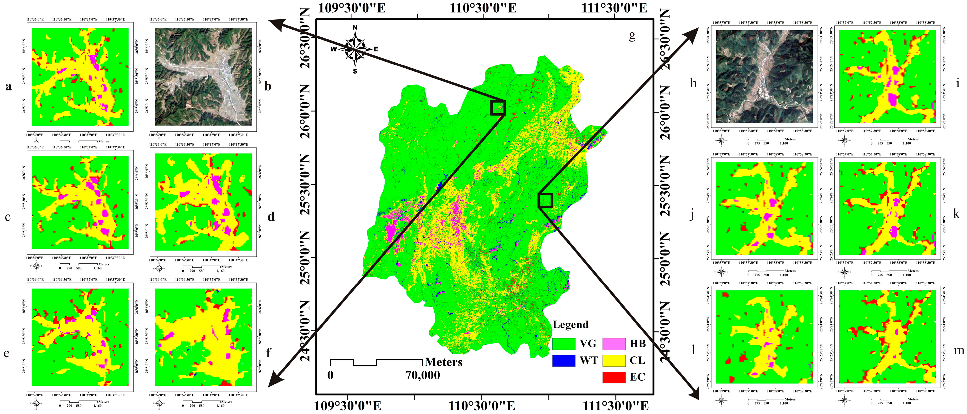
3.1. Datasets
3.2. Non-Spatial Attribute and Spatial Attribute Selection
3.3. Experiments
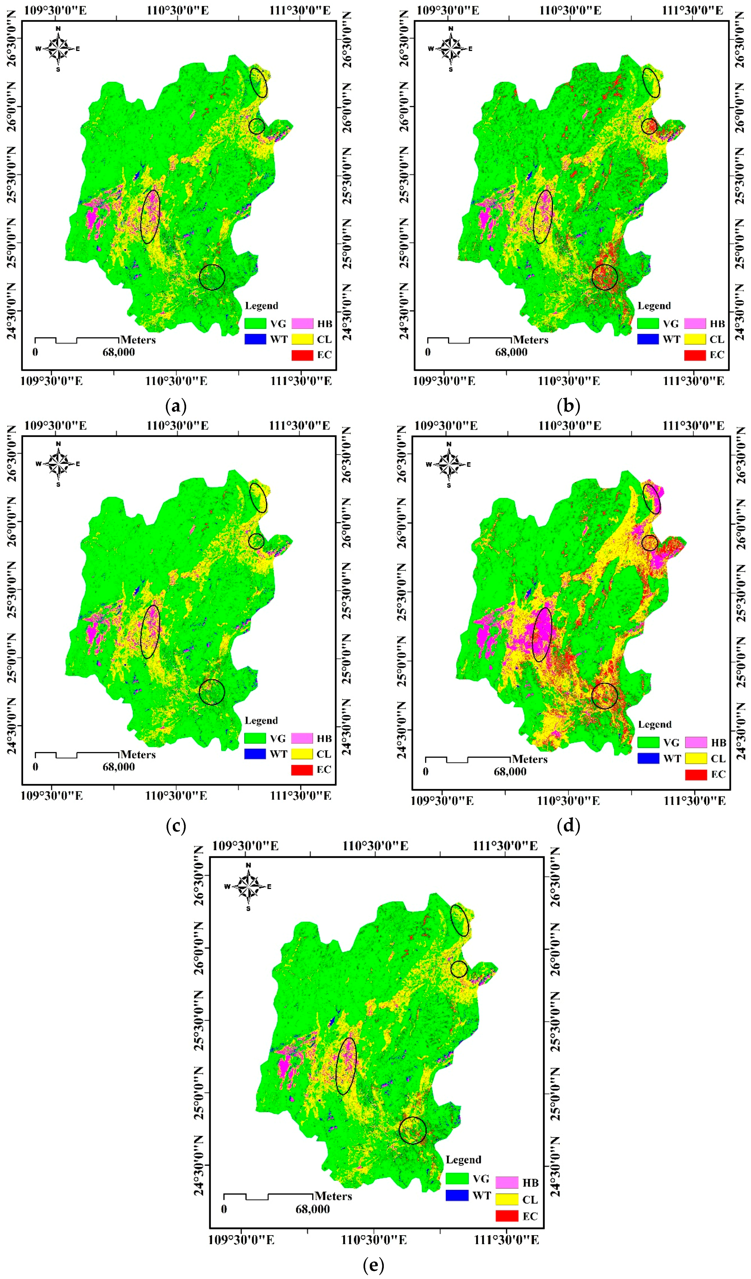
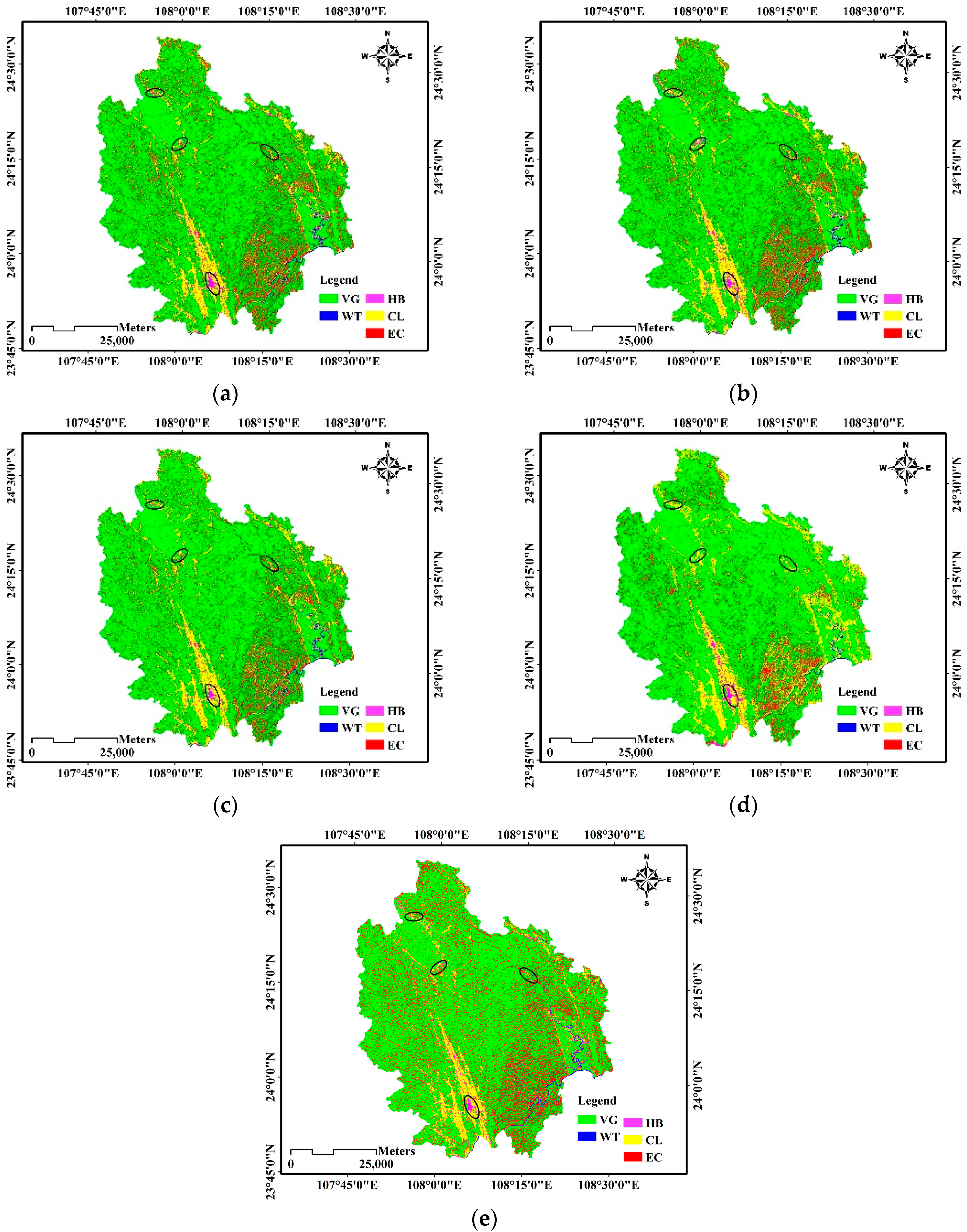
3.3.1. Experiments on the First Test Area
Input Parameters
- Minimum node size: The minimum valid node size can be set in the range of 0–100.
- Maximum purity: If the purity of a node is 95% or higher, the algorithm stops splitting it. Additionally, if its number of records is 1% or less of the total number of records, the algorithm stops splitting it.
- Maximum depth: The maximum valid depth is 20–30.
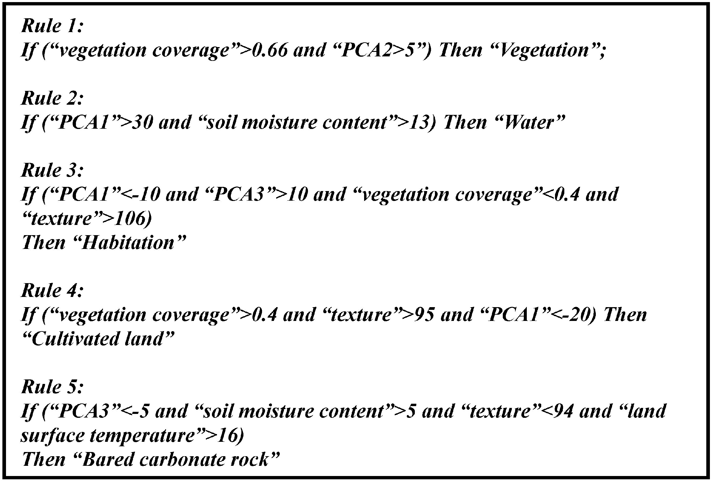
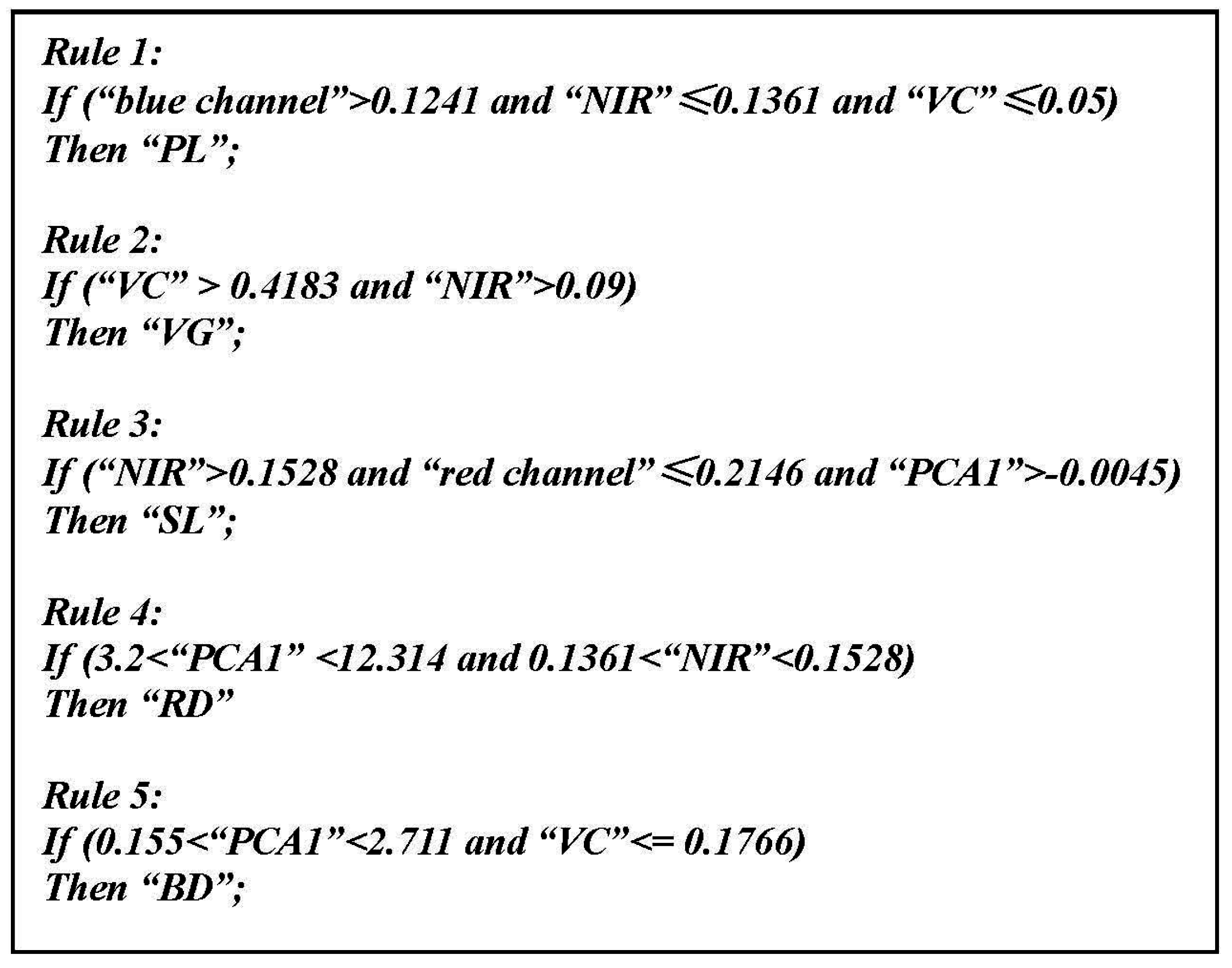
Generation of MVU-based co-location mining rules
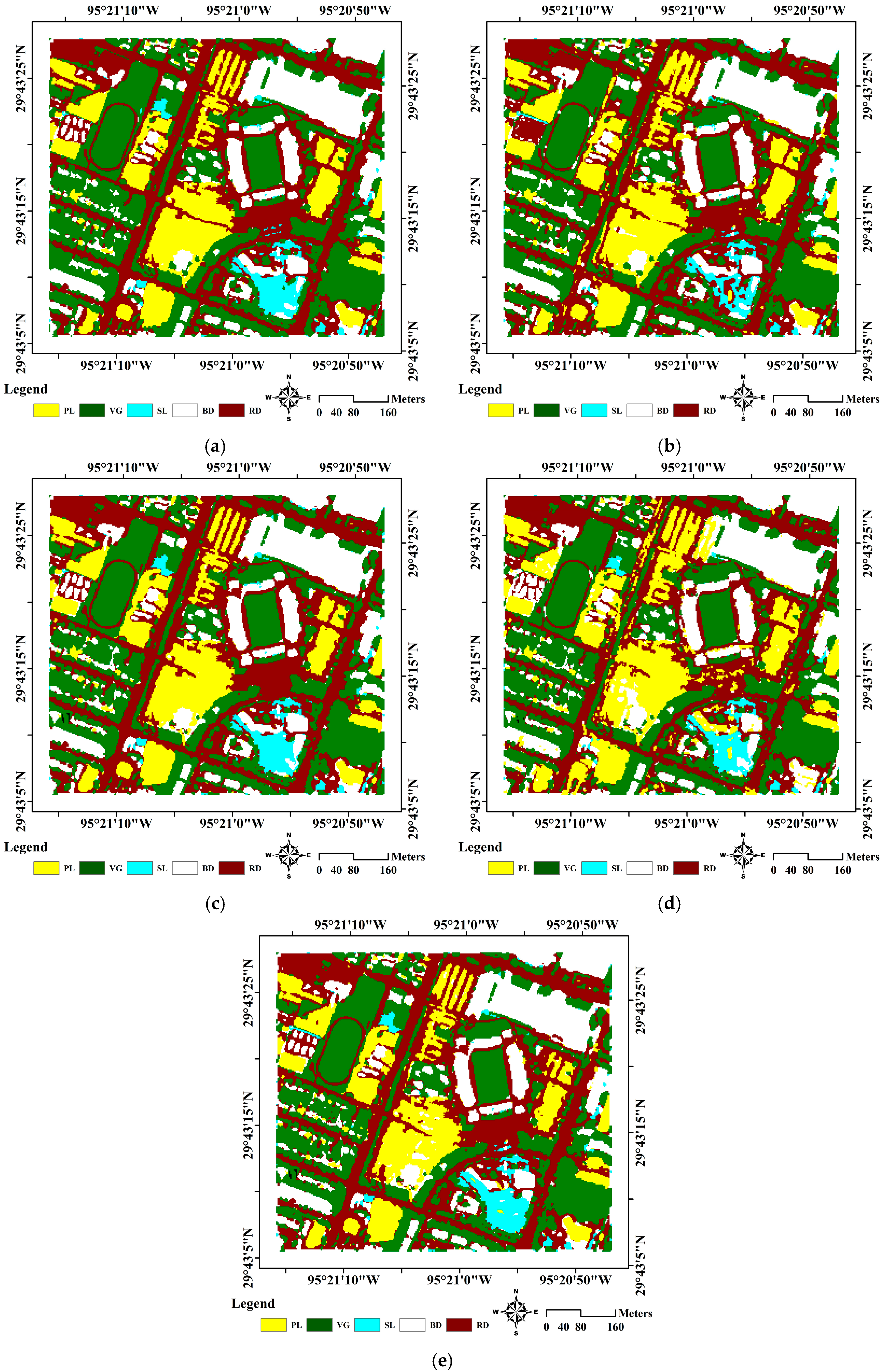
Experimental Results
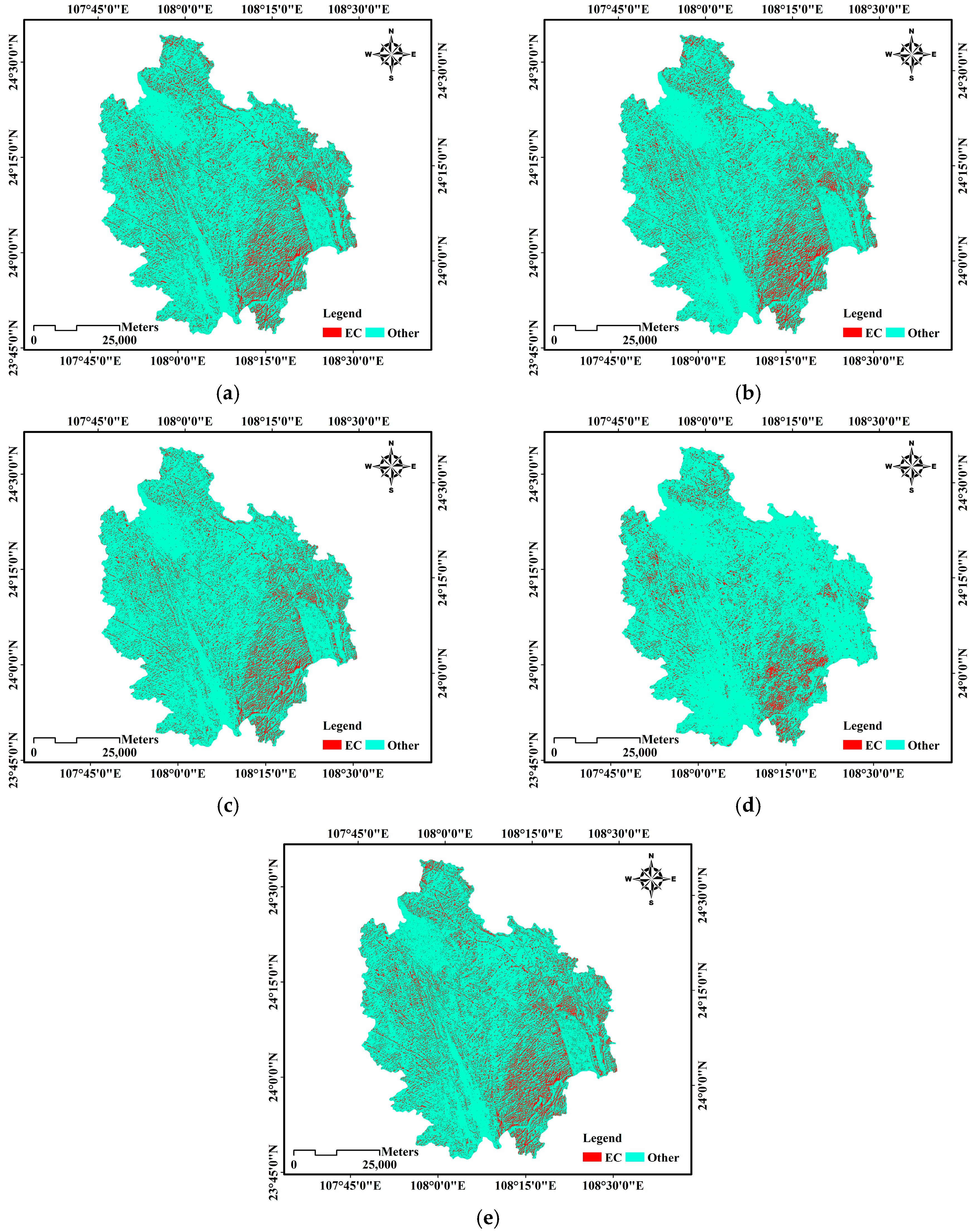
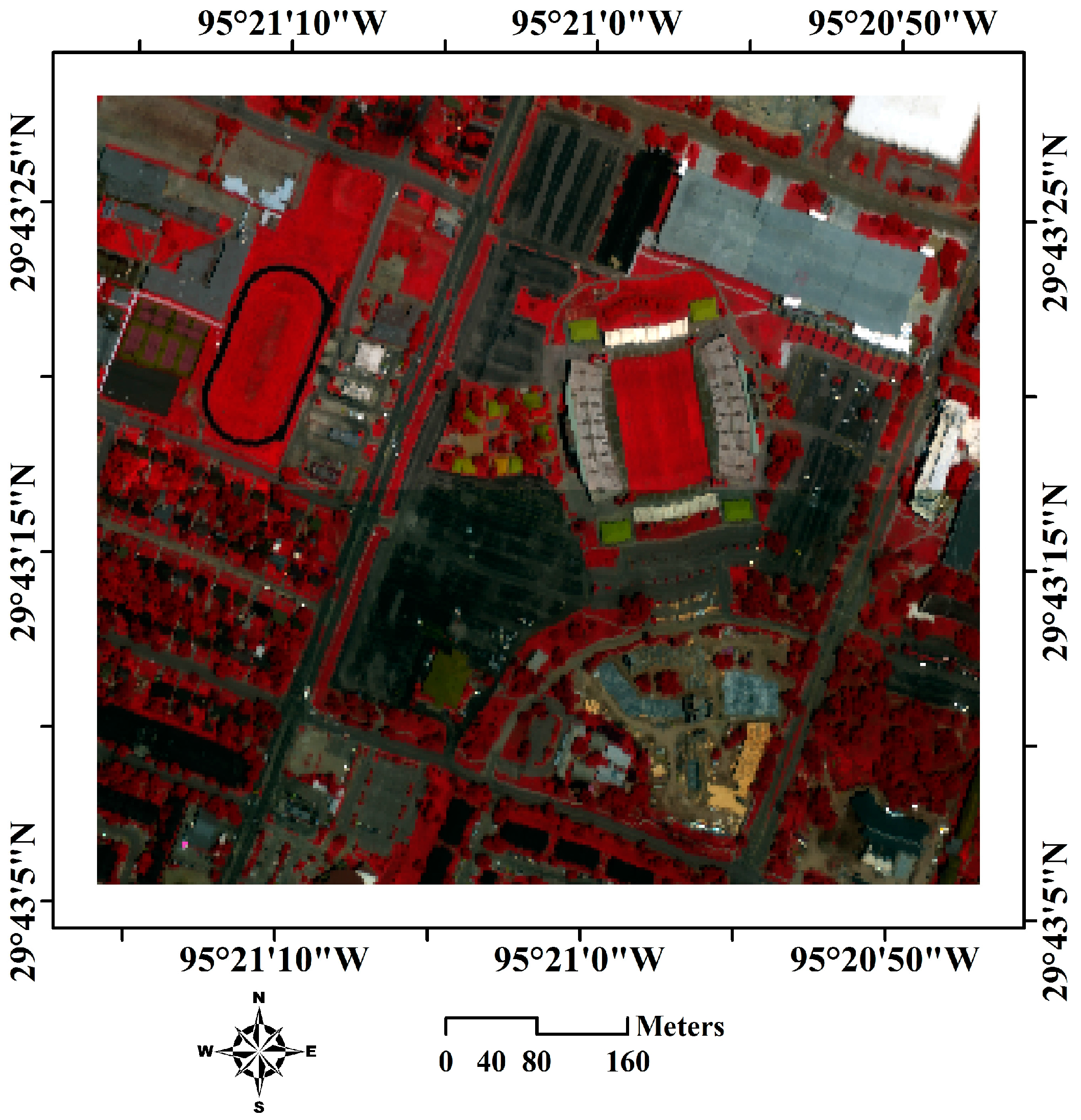
3.3.2. Experiments on the Second Test Area
3.3.3. Experiments on the Third Test Area
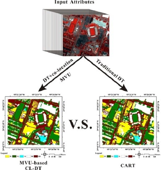
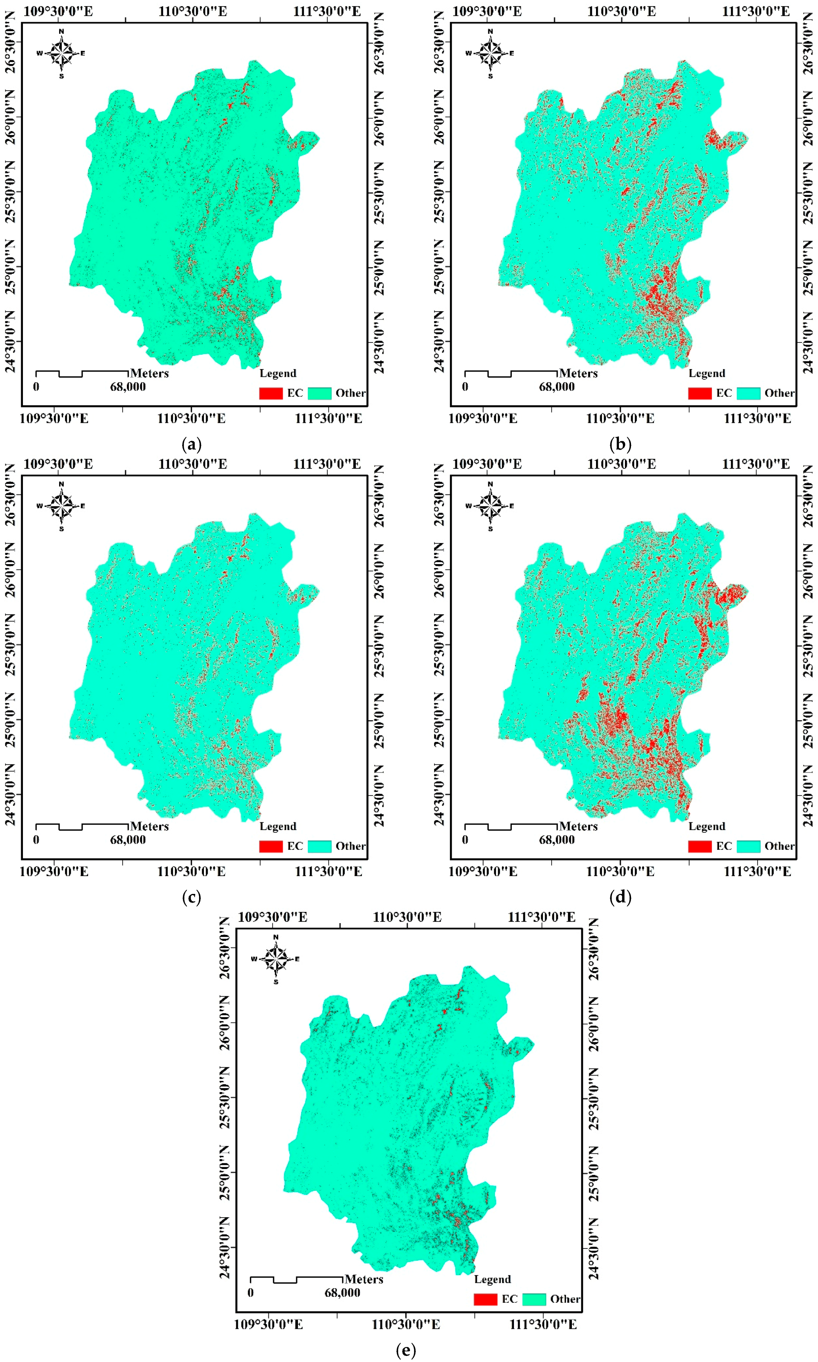
4. Comparison Analysis and Validation in the Field
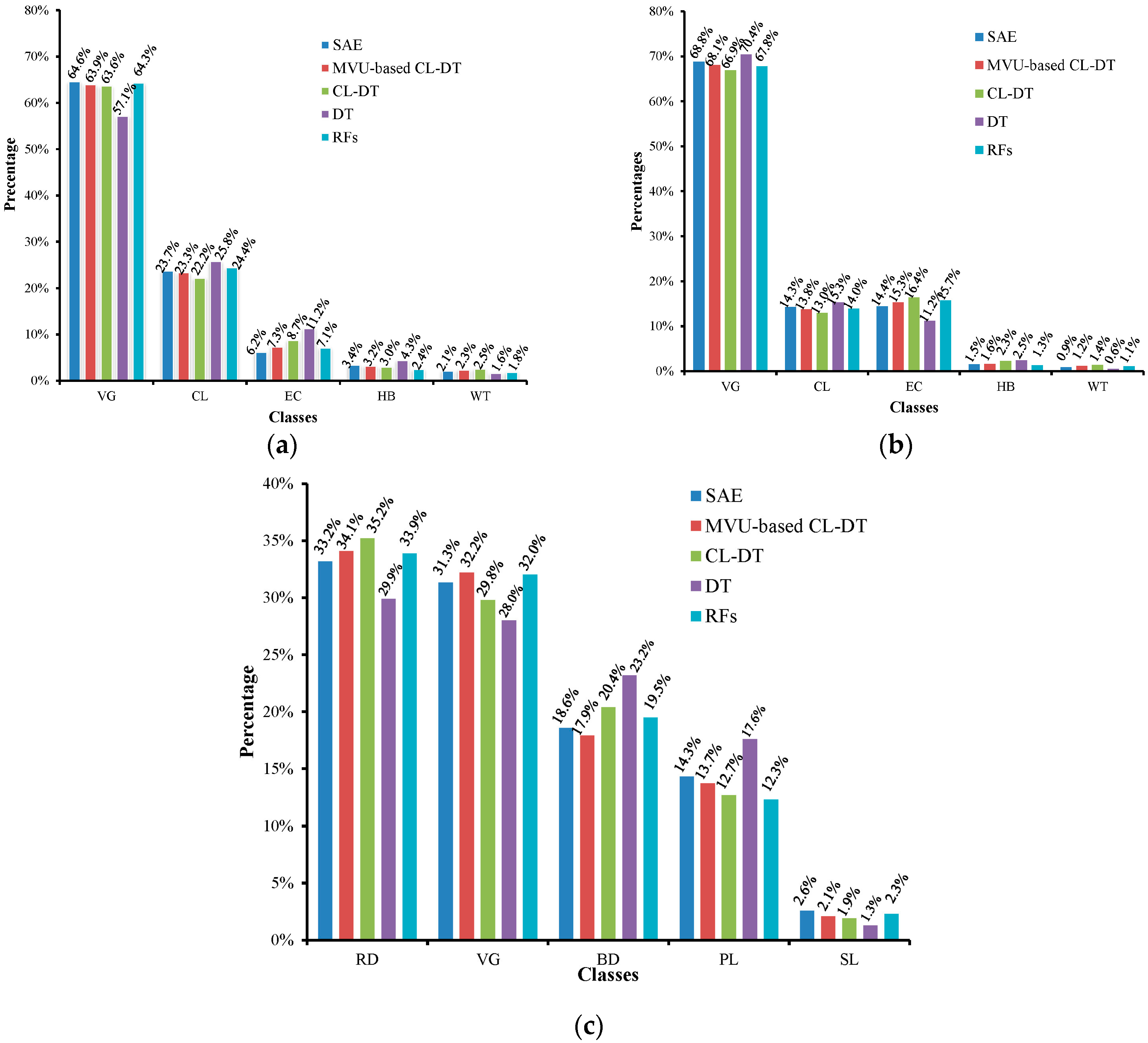
4.1. Classification Accuracy Comparison
4.2. Comparison Analysis for Parameters and Time-Consumption
4.3. Classification Accuracy Validation in the Field
5. Conclusions
Acknowledgments
Author Contributions
Conflicts of Interest
References
- Chen, Y.S.; Lin, Z.H.; Zhao, X.; Wang, G.; Gu, Y.F. Deep learning-based classification of hyperspectral data. IEEE J. Sel. Top. Appl. Earth Obs. Remote Sens. 2014. [Google Scholar] [CrossRef]
- Huang, X.; Zhang, L.P. An SVM ensemble approach combining spectral, structural, and semantic features for the classification of high-resolution remotely sensed imagery. IEEE Trans. Geosci. Remote Sens. 2013, 51, 257–272. [Google Scholar] [CrossRef]
- Huang, X.; Weng, C.L.; Lu, Q.K.; Feng, T.T.; Zhang, L.P. Automatic labelling and selection of training samples for high-resolution remote sensing image classification over urban areas. Remote Sens. 2015, 7, 16024–16044. [Google Scholar] [CrossRef]
- Huang, X.; Lu, Q.K.; Zhang, L.P. A multi-index learning approach for classification of high-resolution remotely sensed images over urban areas. ISPRS J. Photogramm. Remote Sens. 2014, 90, 36–48. [Google Scholar] [CrossRef]
- Simard, M.; Saatehi, S.S.; Grandi, G.D. Use of decision tree and multi-scale texture for classification of JERS-1 SAR data over tropical forest. IEEE Trans. Geosci. Remote Sens. 2000, 38, 2310–2321. [Google Scholar] [CrossRef]
- Franklin, S.E.; Stenhouse, G.B.; Hansen, M.J.; Popplewell, C.C.; Dechka, J.A.; Peddle, D.R. An Integrated Decision Tree Approach (IDTA) to mapping land cover using satellite remote sensing in support of grizzly bear habitat analysis in the Alberta yellow head ecosystem. Can. J. Remote Sens. 2001, 27, 579–592. [Google Scholar] [CrossRef]
- Zhou, G.; Wang, L.; Wang, D.; Reichle, S. Integration of GIS and data mining technology to enhance the pavement management decision making. J. Transp. Eng. 2010, 136, 332–341. [Google Scholar] [CrossRef]
- Xu, C.G.; Anwar, A. Based on the decision tree classification of remote sensing image classification method application. Appl. Mech. Mater. 2013. [Google Scholar] [CrossRef]
- Chasmer, L.; Hopkinson, C.; Veness, T.; Quinton, W.; Baltzer, J. A decision-tree classification for low-lying complex land cover types within the zone of discontinuous permafrost. Remote Sens. Environ. 2014, 143, 73–84. [Google Scholar] [CrossRef]
- Wu, C.; Landgrebe, D.; Swain, P. The Decision Tree Approach to Classification; NASA-CR-141930, LARS-INFORM-NOTE-090174, TR-EE-75-17; Purdue University: West Lafayette, IN, USA, 1 May 1975. [Google Scholar]
- Breiman, L.; Friedman, J.H.; Olshen, R.A.; Stone, C.J. Classification and Regression Trees; Wadsworth International Group: Belmont, CA, USA, 1984. [Google Scholar]
- Quinlan, J.R. Induction of decision trees. Mach. Learn. 1987. [Google Scholar] [CrossRef]
- Quinlan, J.R. C4.5: Programs for Machine Learning; Morgan Kaufmann: San Mateo, CA, USA, 1993. [Google Scholar]
- Bujlow, T.; Riaz, M.T.; Pedersen, J.M. A method for classification of network traffic based on C5.0 machine learning algorithm. In Proceedings of the International Conference on Computing, Networking and Communications (ICNC) 2012, Maui, HI, USA, 30 January–2 February 2012; pp. 237–241.
- Polat, K.; Gunes, S. A novel hybrid intelligent method based on C4.5 decision tree classifier and one-against-all approach for multi-class classification problems. Expert Syst. Appl. 2009, 36, 1587–1592. [Google Scholar] [CrossRef]
- Franco-Arcega, A.; Carrasco-Ochoa, J.A.; Sanchez-Diaz, G.; Martinez-Trinidad, J.F. Decision tree induction using a fast splitting attribute selection for large datasets. Expert Syst. Appl. 2011, 38, 14290–14300. [Google Scholar] [CrossRef]
- Aviad, B.; Roy, G. Classification by clustering decision tree-like classifier based on adjusted clusters. Expert Syst. Appl. 2011. [Google Scholar] [CrossRef]
- Sok, H.K.; Ooi, M.P.; Kuang, Y.C. Sparse alternating decision tree. Pattern Recognit. Lett. 2015. [Google Scholar] [CrossRef]
- Zhou, G.; Wang, L. Co-location decision tree for enhancing decision—Making of pavement maintenance and rehabilitation. Transport. Res. Part C Emerg. Technol. 2012, 21, 287–305. [Google Scholar] [CrossRef]
- Mansour, Y. Pessimistic decision tree pruning based on tree size. In Proceedings of the Fourteenth International Conference on Machine Learning, Nashville, TN, USA, 8–12 July 1997.
- Osei-Bryson, K. Post-pruning in decision tree induction using multiple performance measures. Comput. Oper. Res. 2007, 34, 3331–3345. [Google Scholar] [CrossRef]
- Osei-Bryson, K. Post-pruning in regression tree induction: An integrated approach. Expert Syst. Appl. 2008, 34, 1481–1490. [Google Scholar] [CrossRef]
- Balamurugan, S.A.; Rajaram, R. Effective solution for unhandled exception in decision tree induction algorithms. Expert Syst. Appl. 2009, 36, 12113–12119. [Google Scholar] [CrossRef]
- Appel, R.; Fuchs, T.; Dollar, P.; Peronal, P. Quickly boosting decision trees: Pruning underachieving features early. In Proceedings of the 30th International Conference on Machine Learning, Atlanta, GA, USA, 16–21 June 2013.
- Li, X.; Xing, Q.; Kang, L. Remote sensing image classification method based on evidence theory and decision tree. Proc. SPIE 2010. [Google Scholar] [CrossRef]
- Farid, D.; Zhang, L.; Rahman, C.; Hossain, M.A.; Strachan, R. Hybrid decision tree and naïve Bayes classifiers for multi-class classification tasks. Expert Syst. Appl. 2014, 41, 1937–1946. [Google Scholar] [CrossRef]
- Al-Obeidat, F.; Al-Taani, A.T.; Belacel, N.; Feltrin, L.; Banerjee, N. A fuzzy decision tree for processing satellite images and landsat data. Procedia Comput. Sci. 2015, 52, 1192–1197. [Google Scholar] [CrossRef]
- Zhou, G. Co-location Decision Tree for Enhancing Decision-Making of Pavement Maintenance and Rehabilitation. Ph.D. Thesis, Old Dominion University, Norfolk, VA, USA, 2011. [Google Scholar]
- Zhan, D.; Hua, Z. Ensemble-based manifold learning for visualization. J. Comput. Res. Dev. 2005, 42, 1533–1537. [Google Scholar] [CrossRef]
- Weinberger, K.; Saul, L. Unsupervised learning of image manifolds by semidefinite programming. Int. J. Comput. Vis. 2006, 7, 77–90. [Google Scholar] [CrossRef]
- Wang, J. Maximum Variance Unfolding. In Geometric Structure of High-Dimensional Data and Dimensionality Reduction; Springer: Berlin/Heidelberg, Germany, 2011; pp. 181–202. [Google Scholar]
- Shao, J.D.; Rong, G. Nonlinear process monitoring based on maximum variance unfolding projections. Expert Syst. Appl. 2009, 36, 11332–11340. [Google Scholar] [CrossRef]
- Liu, Y.J.; Chen, T.; Yao, Y. Nonlinear process monitoring and fault isolation using extended maximum variance unfolding. J. Process Control 2014, 24, 880–891. [Google Scholar] [CrossRef]
- Ery, A.C.; Bruno, P. On the convergence of maximum variance unfolding. J. Mach. Learn. Res. 2013, 14, 1747–1770. [Google Scholar]
- Vandenberghe, L.; Boyd, S.P. Semidefinite programming. Soc. Ind. Appl. Math. Rev. 1996, 38, 49–95. [Google Scholar] [CrossRef]
- Weinberger, K.Q.; Packer, B.D.; Saul, L.K. Nonlinear dimensionality reduction by semidefinite programming and kernel matrix factorization. In Proceedings of the Tenth International Workshop on Artificial Intelligence and Statistics (AISTATS-05), Bridgetown, Barbados, 6–8 January 2005; pp. 381–388.
- Kardoulas, N.G.; Bird, A.C.; Lawan, A.I. Geometric correction of spot and Landsat imagery: A comparison of map- and GPS-derived control points. Am. Soc. Photogramm. Remote Sens. 1996, 62, 1171–1177. [Google Scholar]
- Storey, J.C.; Choate, M.J. Landsat-5 Bumper-Mode geometric correction. IEEE Trans. Geosci. Remote Sens. 2004, 42, 2695–2703. [Google Scholar] [CrossRef]
- Yang, W.J. The registration and mosaic of digital image remotely sensed. In Proceedings of the 11th Asian Conference on Remote Sensing, Guangzhou, China, 15–21 November 1990.
- Kanazawaa, Y.; Kanatani, K. Image mosaicing by stratified matching. Image Vision Comput. 2004, 22, 93–103. [Google Scholar] [CrossRef]
- Greiner, G.; Hormann, K. Efficient clipping of arbitrary polygons. ACM Trans. Graph. 1998, 17, 71–83. [Google Scholar] [CrossRef]
- Liu, P.J.; Zhang, L.; Kurban, A. A method for monitoring soil water contents using satellite remote sensing. J. Remote Sens. 1997, 1, 135–139. [Google Scholar]
- Qin, Z.; Karniell, A. A mono-window algorithm for retrieving land surface temperature from Landsat TM data and its application to the Israel-Egypt border region. Int. J. Remote Sens. 2001, 22, 3719–3746. [Google Scholar] [CrossRef]
- Mohammad, A.; Shi, Z.; Ahmad, Y. Application of GIS and remote sensing in soil degradation assessments in the Syrian coast. J. Zhejiang Univ. (Agric. Life Sci.) 2002, 26, 191–196. [Google Scholar]
- Cliff, A.; Ord, J. Spatial Autocorrelation. Environ. Plan. 1973, 7, 725–734. [Google Scholar] [CrossRef]
- Anselin, L. The local indicators of spatial association—LISA. Geog. Anal. 1995, 27, 93–115. [Google Scholar] [CrossRef]
- Getis, A. Spatial autocorrelation. In Handbook of Applied Spatial Analysis: Software Tools, Methods and Applications; Fischer, M., Getis, A., Eds.; Springer: Berlin, Germany, 2010; pp. 255–278. [Google Scholar]
- Zhao, S. Salt Marsh Classification and Extraction Based on HJ NDVI Time Series. Master’s Thesis, Nanjing University, Nanjing, China, May 2015. [Google Scholar]
- Vincent, P.; Larochelle, H.; Lajoie, I.; Bengio, Y.; Manzagol, P. Stacked denoising autoencoders: Learning useful representations in a deep network with a local denoising criterion. J. Mach. Learn. Res. 2010, 11, 3371–3408. [Google Scholar]
- Van der Linden, S.; Rabe, A.; Held, M.; Jakimow, B.; Leitão, P.J.; Okujeni, A.; Schwieder, M.; Suess, S.; Hostert, P. The EnMAP-Box—A toolbox and application programming interface for EnMAP data Processing. Remote Sens. 2015, 7, 11249–11266. [Google Scholar] [CrossRef]


| Description | |
|---|---|
| X/Y coordinates | Projection: Transverse_Mercator |
| False_Easting: 500000.000000 | |
| Central_Meridian: 111.000000 | |
| Scale_Factor: 0.999600 | |
| Latitude_Of_Origin: 0.000000 | |
| Linear Unit: Meter (1.000000) | |
| Geographic Coordinate System: GCS_WGS_1984 | |
| Angular Unit: Degree (0.017453292519943295) | |
| Prime Meridian: Greenwich (0.000000000000) | |
| Datum: D_WGS_1984 |
| VC | PCA1 | TEX | PCA3 | SSM | PCA2 | |
|---|---|---|---|---|---|---|
| Moran’s I | 0.0145 | 0.0173 | 0.0156 | −0.0209 | 0.0222 | −0.0216 |
| z-Score | 0.5902 | 0.7552 | 0.6979 | −0.6713 | 0.8306 | −0.6334 |
| p-value | 0.5549 | 0.4500 | 0.4852 | 0.5020 | 0.4062 | 0.5264 |
| Pattern | RRS | PCA3 | VC | LST | SSM (%) | TEX | DR |
|---|---|---|---|---|---|---|---|
| (2, 3) | Yes | (−20.4, −22.3) | (0.33, 0.15) | (17.2, 16.8) | (4.8, 6.8) | (53.7, 46.3) | 2/5 |
| (3, 4) | Yes | (−22.3, −18.9) | (0.15, 0.13) | (16.8, 16.3) | (6.8, 7.6) | (46.3, 45.7) | 1 |
| (10, 15) | Yes | (−17.2, −20.8) | (0.21, 0.24) | (16.9, 16.8) | (9.8, 5.3) | (58.7, 46.5) | 3/5 |
| (11, 12, 16) | Yes | (−19.3, −19.8, −21.2) | (0.21, 0.19, 0.24) | (16.5, 17.1, 16.6) | (6.1, 7.4, 6.7) | (47.6, 46.6, 6.9) | 1 |
| SAE (Baseline) | DT | CL-DT | RFs | MVU-Based CL-DT | |
|---|---|---|---|---|---|
| RD (%) | 0 | 25.32 | 16.38 | 9.43 | 8.93 |
| RA (%) | 100 | 74.68 | 83.62 | 90.57 | 91.07 |
| SAE (Baseline) | DT | CL-DT | RFs | MVU-Based CL-DT | |
|---|---|---|---|---|---|
| RD (%) | 0 | 25.03 | 14.72 | 9.08 | 8.46 |
| RA (%) | 100 | 74.97 | 85.28 | 90.92 | 91.54 |
| SAE (Baseline) | DT | CL-DT | RFs | MVU-Based CL-DT | |
|---|---|---|---|---|---|
| RD (%) | 0 | 15.89 | 7.77 | 4.62 | 3.61 |
| RA (%) | 100 | 84.11 | 92.23 | 95.38 | 96.39 |
| VG | WT | EC | HB | CL | PA | UA | |
|---|---|---|---|---|---|---|---|
| VG | 967 | 49 | 38 | 0 | 65 | 0.967 | 0.864 |
| WT | 0 | 945 | 0 | 0 | 0 | 0.945 | 1.00 |
| EC | 29 | 2 | 839 | 42 | 74 | 0.839 | 0.850 |
| HB | 0 | 0 | 0 | 958 | 0 | 0.958 | 1.00 |
| CL | 4 | 4 | 123 | 0 | 861 | 0.861 | 0.868 |
| AA | 0.914 | 0.916 |
| VG | WT | EC | HB | CL | PA | UA | |
|---|---|---|---|---|---|---|---|
| VG | 918 | 7 | 29 | 0 | 77 | 0.918 | 0.890 |
| WT | 0 | 967 | 0 | 0 | 0 | 0.967 | 1.00 |
| EC | 65 | 0 | 809 | 65 | 32 | 0.809 | 0.833 |
| HB | 8 | 6 | 25 | 929 | 8 | 0.929 | 0.952 |
| CL | 9 | 20 | 137 | 6 | 883 | 0.883 | 0.837 |
| AA | 0.901 | 0.902 |
| PL | VG | SL | BD | RD | PA | UA | |
|---|---|---|---|---|---|---|---|
| PL | 25 | 0 | 0 | 2 | 3 | 0.833 | 0.833 |
| VG | 0 | 30 | 0 | 0 | 0 | 1.00 | 1.00 |
| SL | 1 | 0 | 23 | 0 | 1 | 0.767 | 0.920 |
| BD | 2 | 0 | 4 | 27 | 0 | 0.900 | 0.818 |
| RD | 2 | 0 | 3 | 1 | 26 | 0.867 | 0.837 |
| AA | 0.873 | 0.882 |
| VG | WT | EC | HB | CL | PA | UA | |
|---|---|---|---|---|---|---|---|
| VG | 864 | 46 | 61 | 0 | 29 | 0.864 | 0.864 |
| WT | 9 | 893 | 0 | 56 | 13 | 0.893 | 0.920 |
| EC | 37 | 9 | 793 | 169 | 119 | 0.793 | 0.704 |
| HB | 23 | 31 | 4 | 753 | 0 | 0.753 | 0.928 |
| CL | 67 | 21 | 142 | 22 | 839 | 0.839 | 0.769 |
| AA | 0.828 | 0.837 |
| VG | WT | EC | HB | CL | PA | UA | |
|---|---|---|---|---|---|---|---|
| VG | 864 | 53 | 137 | 48 | 62 | 0.864 | 0.742 |
| WT | 12 | 909 | 0 | 24 | 73 | 0.909 | 0.893 |
| EC | 28 | 7 | 753 | 27 | 107 | 0.753 | 0.817 |
| HB | 19 | 2 | 67 | 819 | 8 | 0.819 | 0.895 |
| CL | 77 | 29 | 43 | 82 | 750 | 0.750 | 0.765 |
| AA | 0.819 | 0.822 |
| PL | VG | SL | BD | RD | PA | UA | |
|---|---|---|---|---|---|---|---|
| PL | 22 | 0 | 0 | 2 | 5 | 0.733 | 0.759 |
| VG | 0 | 29 | 0 | 1 | 0 | 0.967 | 0.967 |
| SL | 2 | 1 | 24 | 0 | 1 | 0.800 | 0.857 |
| BD | 2 | 0 | 3 | 25 | 1 | 0.833 | 0.807 |
| RD | 4 | 0 | 3 | 2 | 23 | 0.767 | 0.719 |
| AA | 0.820 | 0.822 |
| VG | WT | EC | HB | CL | PA | UA | |
|---|---|---|---|---|---|---|---|
| VG | 1000 | 41 | 25 | 5 | 29 | 1.00 | 0.909 |
| WT | 0 | 728 | 0 | 6 | 4 | 0.728 | 0.987 |
| EC | 0 | 115 | 793 | 131 | 241 | 0.793 | 0.619 |
| HB | 0 | 109 | 57 | 847 | 92 | 0.847 | 0.766 |
| CL | 0 | 7 | 125 | 11 | 634 | 0.634 | 0.816 |
| AA | 0.800 | 0.819 |
| VG | WT | EC | HB | CL | PA | UA | |
|---|---|---|---|---|---|---|---|
| VG | 953 | 4 | 47 | 0 | 0 | 0.953 | 0.949 |
| WT | 0 | 954 | 0 | 0 | 0 | 0.954 | 1.00 |
| EC | 45 | 31 | 500 | 100 | 18 | 0.500 | 0.720 |
| HB | 0 | 0 | 0 | 713 | 0 | 0.713 | 1.00 |
| CL | 2 | 11 | 453 | 187 | 982 | 0.982 | 0.601 |
| AA | 0.820 | 0.854 |
| PL | VG | SL | BD | RD | PA | UA | |
|---|---|---|---|---|---|---|---|
| PL | 22 | 0 | 1 | 0 | 8 | 0.733 | 0.710 |
| VG | 0 | 27 | 0 | 2 | 0 | 0.900 | 0.931 |
| SL | 1 | 2 | 21 | 0 | 0 | 0.700 | 0.875 |
| BD | 0 | 1 | 7 | 23 | 1 | 0.767 | 0.719 |
| RD | 7 | 0 | 1 | 5 | 21 | 0.700 | 0.618 |
| AA | 0.760 | 0.771 |
| VG | WT | EC | HB | CL | PA | UA | |
|---|---|---|---|---|---|---|---|
| VG | 996 | 0 | 0 | 0 | 0 | 0.996 | 1.00 |
| WT | 0 | 1000 | 19 | 0 | 0 | 1.00 | 0.981 |
| EC | 4 | 0 | 893 | 53 | 24 | 0.893 | 0.917 |
| HB | 0 | 0 | 88 | 947 | 0 | 0.947 | 0.915 |
| CL | 0 | 0 | 0 | 0 | 976 | 0.976 | 1.00 |
| AA | 0.962 | 0.963 |
| VG | WT | EC | HB | CL | PA | UA | |
|---|---|---|---|---|---|---|---|
| VG | 1000 | 0 | 15 | 0 | 23 | 1.00 | 0.963 |
| WT | 0 | 1000 | 0 | 0 | 0 | 1.00 | 1.00 |
| EC | 0 | 0 | 954 | 14 | 120 | 0.954 | 0.877 |
| HB | 0 | 0 | 10 | 986 | 4 | 0.986 | 0.986 |
| CL | 0 | 0 | 21 | 0 | 853 | 0.853 | 0.976 |
| AA | 0.959 | 0.960 |
| PL | VG | SL | BD | RD | PA | UA | |
|---|---|---|---|---|---|---|---|
| PL | 26 | 0 | 0 | 1 | 2 | 0.866 | 0.897 |
| VG | 0 | 30 | 0 | 0 | 0 | 1.00 | 1.00 |
| SL | 1 | 0 | 25 | 0 | 1 | 0.833 | 0.926 |
| BD | 2 | 0 | 2 | 28 | 0 | 0.933 | 0.875 |
| RD | 1 | 0 | 3 | 1 | 27 | 0.900 | 0.844 |
| AA | 0.906 | 0.908 |
| VG | WT | EC | HB | CL | PA | UA | |
|---|---|---|---|---|---|---|---|
| VG | 949 | 0 | 19 | 0 | 31 | 0.949 | 0.950 |
| WT | 2 | 964 | 0 | 6 | 7 | 0.964 | 0.985 |
| EC | 14 | 0 | 819 | 63 | 116 | 0.819 | 0.809 |
| HB | 0 | 27 | 49 | 931 | 0 | 0.931 | 0.925 |
| CL | 35 | 9 | 113 | 0 | 846 | 0.846 | 0.843 |
| AA | 0.902 | 0.902 |
| VG | WT | EC | HB | CL | PA | UA | |
|---|---|---|---|---|---|---|---|
| VG | 932 | 13 | 24 | 0 | 17 | 0.932 | 0.945 |
| WT | 0 | 944 | 0 | 19 | 0 | 0.944 | 0.980 |
| EC | 24 | 0 | 838 | 35 | 112 | 0.838 | 0.831 |
| HB | 11 | 31 | 17 | 937 | 10 | 0.937 | 0.931 |
| CL | 33 | 12 | 121 | 9 | 861 | 0.861 | 0.832 |
| AA | 0.902 | 0.904 |
| PL | VG | SL | BD | RD | PA | UA | |
|---|---|---|---|---|---|---|---|
| PL | 24 | 0 | 2 | 1 | 3 | 0.80 | 0.80 |
| VG | 0 | 29 | 0 | 0 | 0 | 0.967 | 1.00 |
| SL | 1 | 1 | 24 | 0 | 2 | 0.80 | 0.857 |
| BD | 3 | 0 | 2 | 28 | 0 | 0.933 | 0.848 |
| RD | 2 | 0 | 2 | 1 | 25 | 0.833 | 0.833 |
| AA | 0.867 | 0.868 |
| 1st Test Area | 2nd Test Area | 3rd Test Area | ||||
|---|---|---|---|---|---|---|
| OA | KC | OA | KC | OA | KC | |
| Our method | 91.40% | 0.89 | 90.12% | 0.87 | 87.34% | 0.84 |
| CL-DT | 82.84% | 0.79 | 81.80% | 0.77 | 82.0% | 0.78 |
| SAE | 96.24% | 0.95 | 95.86% | 0.94 | 90.66% | 0.88 |
| CRAT | 80.04% | 0.75 | 82.04% | 0.78 | 76.0% | 0.70 |
| RFs | 90.18% | 0.88 | 90.24% | 0.88 | 86.67% | 0.83 |
| DT | CL-DT | Our Method | |
|---|---|---|---|
| Total number of nodes | 25 | 21 | 11 |
| Number of leaf nodes | 13 | 11 | 6 |
| Number of levels | 9 | 8 | 6 |
| Time Taken (Seconds) | |||
|---|---|---|---|
| DT | CL-DT | Our Method | |
| Data processing | 6 | 4 | 3 |
| Decision tree growing | 11 | 8 | 5 |
| Decision tree drawing | 22 | 18 | 10 |
| Generating rules | 52 | 37 | 21 |
| Latitude | Longitude | Latitude | Longitude | ||
|---|---|---|---|---|---|
| 1 | 25°36′11.52″ | 111°6′38.88″ | 11 | 25°36′39.45″ | 111°6′49.18″ |
| 2 | 25°36′20.29″ | 111°6′47.49″ | 12 | 25°36′38.63″ | 111°6′53.45″ |
| 3 | 25°36′17.86″ | 111°6′39.42″ | 13 | 25°36′32.58″ | 111°6′47.21″ |
| 4 | 25°36′25.42″ | 111°6′38.86″ | 14 | 25°36′39.41″ | 111°6′57.76″ |
| 5 | 25°36′26.88″ | 111°6′41.03″ | 15 | 25°36′33.75″ | 111°6′44.85″ |
| 6 | 25°36′25.66″ | 111°6′1.01″ | 16 | 25°36′37.07″ | 111°6′51.73″ |
| 7 | 25°36′33.95″ | 111°6′48.99″ | 17 | 25°36′40.58″ | 111°6′32.31″ |
| 8 | 25°36′35.41″ | 111°6′51.41″ | 18 | 25°36′41.16″ | 111°6′36.61″ |
| 9 | 25°36′37.85″ | 111°6′48.72″ | 19 | 25°36′32.56″ | 111°6′37.25″ |
| 10 | 25°36′36.39″ | 111°6′47.11″ | 20 | 25°36′25.92″ | 111°6′45.42″ |
© 2016 by the authors; licensee MDPI, Basel, Switzerland. This article is an open access article distributed under the terms and conditions of the Creative Commons Attribution (CC-BY) license (http://creativecommons.org/licenses/by/4.0/).
Share and Cite
Zhou, G.; Zhang, R.; Zhang, D. Manifold Learning Co-Location Decision Tree for Remotely Sensed Imagery Classification. Remote Sens. 2016, 8, 855. https://doi.org/10.3390/rs8100855
Zhou G, Zhang R, Zhang D. Manifold Learning Co-Location Decision Tree for Remotely Sensed Imagery Classification. Remote Sensing. 2016; 8(10):855. https://doi.org/10.3390/rs8100855
Chicago/Turabian StyleZhou, Guoqing, Rongting Zhang, and Dianjun Zhang. 2016. "Manifold Learning Co-Location Decision Tree for Remotely Sensed Imagery Classification" Remote Sensing 8, no. 10: 855. https://doi.org/10.3390/rs8100855
APA StyleZhou, G., Zhang, R., & Zhang, D. (2016). Manifold Learning Co-Location Decision Tree for Remotely Sensed Imagery Classification. Remote Sensing, 8(10), 855. https://doi.org/10.3390/rs8100855