Article

Discrimination of Settlement and Industrial Area Using Landscape Metrics in Rural Region

1
Institute of Agriculture Remote Sensing and Information Technology, College of Environmental and Resource Sciences, Zhejiang University, Hangzhou 310058, China
2
Institute of Zhejiang Land Surveying and Planning, Hangzhou 310007, China
*
Authors to whom correspondence should be addressed.
Remote Sens. 2016, 8(10), 845; https://doi.org/10.3390/rs8100845
Submission received: 27 July 2016 / Revised: 27 September 2016 / Accepted: 11 October 2016 / Published: 15 October 2016

Abstract

:
Detailed and precise information of land-use and land-cover (LULC) in rural area is essential for land-use planning, environment and energy management. The confusion in mapping residential and industrial areas brings problems in energy management, environmental management and sustainable land use development. However, they remain ambiguous in the former rural LULC mapping, and this insufficient supervision leads to inefficient land exploitation and a great waste of land resources. Hence, the extent and area of residential and industrial cover need to be revealed urgently. However, spectral and textural information is not sufficient for classification heterogeneity due to the similarity between different LULC types. Meanwhile, the contextual information about the relationship between a LULC feature and its surroundings still has potential in classification application. This paper attempts to discriminate settlement and industry area using landscape metrics. A feasible classification scheme integrating landscape metrics, chessboard segmentation and object-based image analysis (OBIA) is proposed. First LULC map is generated from GeoEye-1 image, which delineated distribution of different land-cover materials using traditional OBIA method with spectrum and texture information. Then, a chessboard segmentation of the whole LULC map is conducted to create landscape units in a uniform spatial area. Landscape characteristics in each square of chessboard are adopted in the classification algorithm subsequently. To analyze landscape unit scale effect, a variety of chessboard scales are tested, with overall accuracy ranging from 75% to 88%, and Kappa coefficient from 0.51 to 0.76. Optimal chessboard scale is obtained through accuracy assessment comparison. This classification scheme is then compared to two other approaches: a top-down hierarchical classification network using only spectral, textural and shape properties, and lacunarity based hierarchical classification. The distinction approach proposed is overwhelming by achieving the highest value in overall accuracy, Kappa coefficient and McNemar test. The results show that landscape properties from chessboard segment squares could provide valuable information in classification.

Graphical Abstract

1. Introduction

Remote sensing data have provided valuable and abundant sources of information for terrestrial land-use and land-cover (LULC) interpretation and change detection for decades [1,2]. Since the application of a series of very high resolution (VHR) Imagery range from IKONOS, QuickBird, WorldView and Geoeye, these metric or sub-metric resolution sensor data have become the main data source in LULC information extraction [3,4], change monitoring [5,6], land-use planning [7] and so on. Most of these studies focus on urban are, suburban area or the urban–rural interface, while few of them pay attention to rural area or agricultural land [8].
Detailed information regarding the land-use type, spatial area and distribution of buildings within rural regions is in urgent need for effective land resource management, energy supply management, environmental management and policy making. Residential and industrial building type remain ambiguous in current rural LULC maps. This circumstance impedes the process of precisely mapping rural areas for sustainable land-use development. Insufficient supervision on settlement and industry land leads to a tremendous waste of land resources and inefficient land exploitation within agricultural land.
Compared to urban land-cover types, rural land-cover categories have specific characteristics. Rural regions contain a larger number of vegetation cover or non-built cover than cities. In rural land, artificial surfaces such as rooftops, settlements, agricultural facilities, roads, etc., are sparse and have smaller occupied area.
Due to the fine spatial resolution, it becomes possible to identify the minimum feature such as a single rooftop in remotely sensed VHR imagery. Thus, VHR images could provide timely and tangible information for automatically subdividing rural settlement and industrial land-use types. Object-based image analysis (OBIA) fills the gap between pixels and real-world land cover objects [9], which is similar to human perception [10], and was proven to have produced a significantly higher accuracy than traditional pixel-based classification approaches employed in VHR images.
The processing units in OBIA method are not pixels but objects after segmentation, therefore a number of object features characterizing the spatial and textural information can be exploited to facilitate mapping accuracy [9]. Previous studies have demonstrated that textural features [11,12], gray-level co-occurrence matrix (GLCM) [13], local indicators of spatial association (LISA) [14] information and local spatial statistics [11] can be considered as features in OBIA classification procedures.
Furthermore, spatial and textural properties extracted from the image objects in object-based image analysis was proven to have made valuable contributions in discrimination or distinction heterogeneity among land-use categories that are difficult to distinguish, e.g., different land-use types with similar land-cover, or same land-use types with distinct spatial distribution pattern. For settlement or residential building discrimination purpose, Niebergall [15] presented a hierarchical network embedding GLCM to distinguish between different settlement structures as well as land-cover classes. Owen’s research [3] demonstrates that land-cover surface texture and geomorphic properties are significantly different between squatter settlements in suburban areas and well-established settlements in urban areas. Some researchers invented new index for distinguishing building types, particularly in rural areas. Kuffer [16] used unplanned settlement index (USI), which integrated morphological features to distinguish between planned and unplanned areas from VHR data. Vegetation sample-based vegetation index, chessboard segmentation and average contrast of objects were used for extraction of plantation [17].
This spectral and textural information mentioned above was derived from the object itself, and the contextual information about the relationship between the object and its surroundings or circumstances still has potential in classification application. Han [14,18] proposed a multi-scale approach incorporating textural and contextual information in hierarchical network of image objects to analyze of forest ecosystems of a complex nature.
Moreover, by using contextual information, some researchers used spatial statistics methods to improve discrimination techniques, such as local indicators of spatial association (LISA) measures, effective mesh size [19] and lacunarity. Lacunarity was used to identify informal settlements from a high resolution binary imagery [20]. Ma [21] successfully discriminated residential and industrial buildings by integrating lacunarity algorithm, object-based segmentation and a decision tree classifier.
Different land-use behaviors will form different land-use units, which have different landscape pattern characteristics [22]. In addition to spatial statistical methods for describing the landscape pattern, there are other means such as landscape metrics. Landscape metrics were designed to quantify the pattern of the landscape within the designated landscape spatial unit [23]. In other words, landscape metrics contain the information of relationship between different land-use features. Therefore, landscape metrics have the potential to be integrated into the object-based classification. Facilitated by recent advances in computer processing and geographic information (GIS) technologies, a variety of landscape metrics have been developed for calculate landscape pattern [24], including metrics describe area, edge, shape, aggregation and diversity in path level, class level and landscape level [23]. Although these metrics were not designed for the classification phase of image processing, some studies have suggested and succeeded in using landscape metrics for image classification [19,25].
This paper applied landscape metrics to discriminate settlement and industry landscape units. After land-cover map is derived from VHR image, a chessboard segmentation was used to generate uniform landscape spatial units. Landscape metrics that characterize area proportion, shape, edge, aggregation and diversity properties were collected and adopted in classification algorithm. Three different classification schemes are compared: the method proposed, hierarchical classification using only spectral and textural properties, and hierarchical classification integrating lacunarity algorithm.

2. Study Area and Data
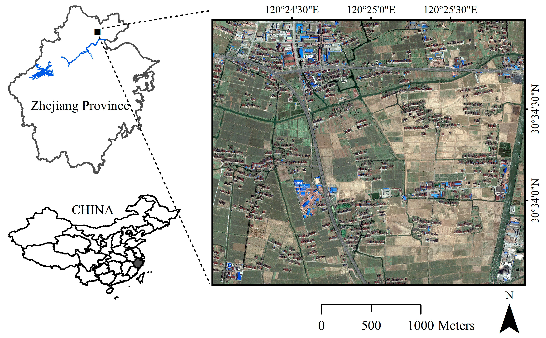
2.1. Study Area

In this study, we selected a typical rural region in the Yangtze River Delta. The study site includes three villages located in Chongfu Town and Shimeng Town, Tongxiang County, Zhejiang Province (120°24′45″E, 30°34′00″W, Figure 1). The region has a subtropical climate with a clear monsoonal character and four distinct seasons. The annual average temperature and total annual precipitation are approximately 16.5 °C and 1246.7 mm, respectively [26]. Due to the excellent climate and soil conditions, various crops are suitable to grow in study area. This place was the traditional main grain producing area of China for millennia. Nevertheless, massive scale industrialization and rapid development have taken place since the 1990s. This study site also includes Economic and Technological Development Zones (ETDZs) of Shimeng Town, which have over 60 companies and beyond 5000 employees [26]. Therefore, this area represents a typical landscape of township economic prosperity and development in a rural region of Eastern China.
This area includes natural or semi-natural land cover materials (e.g., water, trees/shrubs, bare soil, and crops) and various anthropogenic material features (e.g., asphalt, concrete roads/parking lots and different roof top materials, Figure 2). A category schema was developed that detailed land-cover heterogeneity throughout the rural area. The land-cover classes identified were: asphalt, concrete (including rooftops, grain-sunning ground, roads and parking lots), clay rooftops (including dark or red color rooftops both from settlement and industry buildings), metal rooftops (mainly blue rooftops of warehouse and factory), farmland, trees and shrubs, bare soil, and water.

2.2. Data and Preprocessing
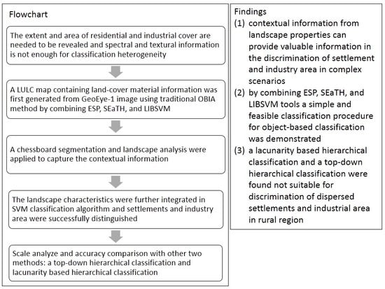
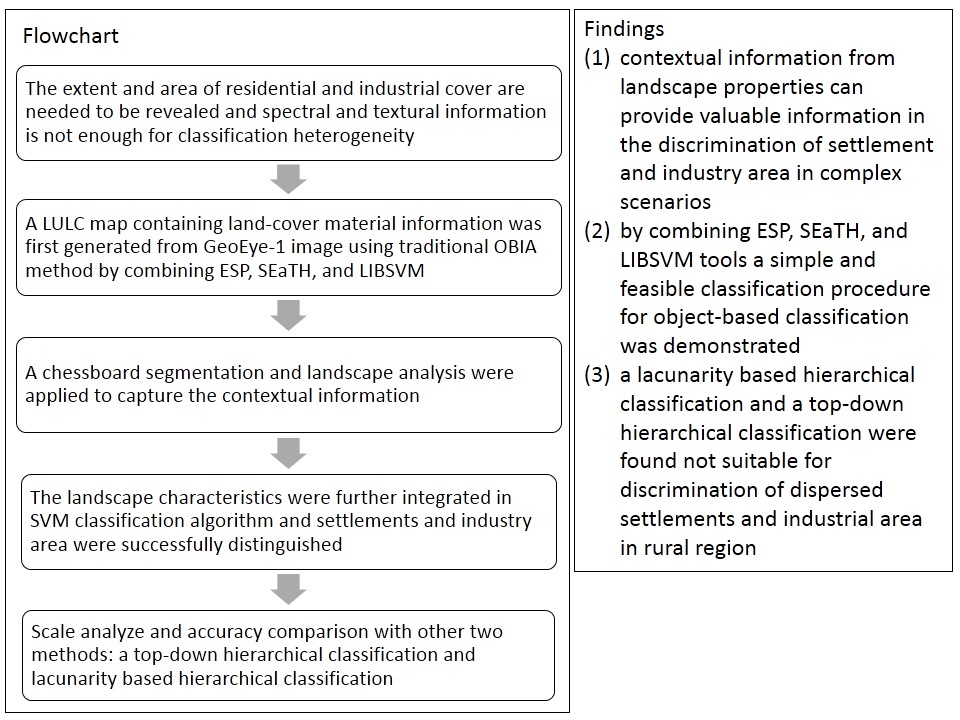
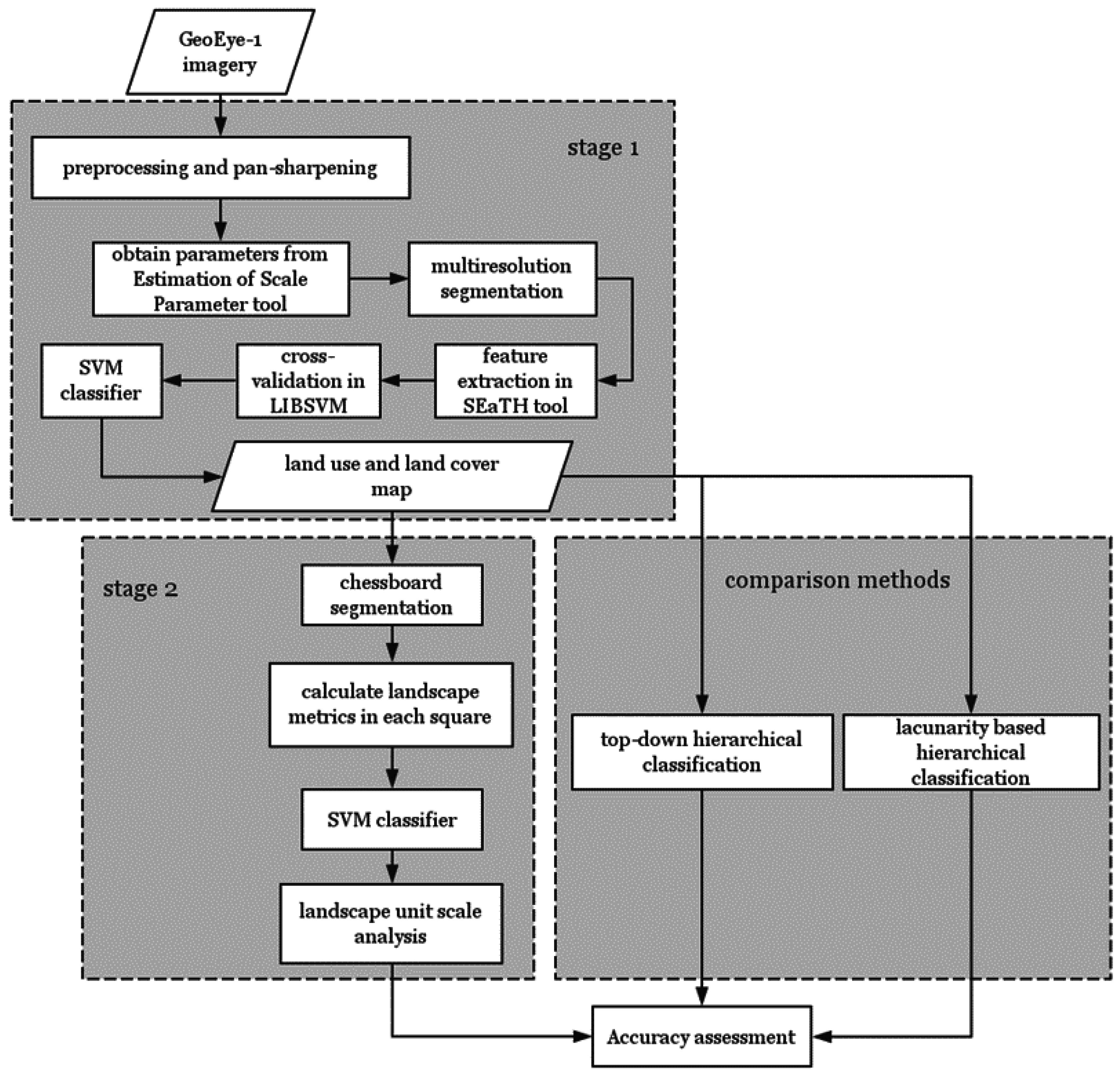
This study used a GeoEye-1 image acquired on 12 May 2010 with multispectral bands (MSI) in spatial resolution of 2 m and a panchromatic band (PAN) in high spatial resolution of 0.5 m.
The image was radiometric corrected by the data provider (GeoEye Imagery Collection Systems Inc., Dulles, VA, USA), and was orthorectified into the Universal Transverse Mercator (UTM) projection system. For the cloud-free atmospheric condition in whole image, there was no need for atmospheric correction in preprocessing step. Gram–Schmidt pan-sharpening method (ENVI, ITT Visual Information Systems, Version 5.1) was used to fuse the multispectral and panchromatic bands. To cover the study area, a rectangle subset of the image was used in segmentation and classification steps, subsequently. Due to its fine spatial resolution, the image data are still sizeable (5500 rows × 6500 columns). Except the original bands, Normalized Difference Vegetation Index (NDVI) was used in the analysis.
In addition to the above raster data, ancillary data were collected in this study. Land-use maps from the National Detailed Land-use Inventory in 2011 were employed in image processing step and accuracy assessment. These land-use maps were derived by visual interpretation on sub-metric resolution aerial photograph and been corrected by ground survey.

3. Methodology

The classification approach we proposed is twofold. Land-cover information was derived in Stage 1, and settlements and industry area was distinguished in Stage 2. In order to verify whether the proposed method can effectively improve the classification accuracy, this study also used other two classification methods based on the result from Stage 1:
  • Top-down hierarchical classification network using only spectral, textural and shape properties; and
  • Hierarchical classification integrating lacunarity properties.
The whole network of classification is illustrated in Figure 3. Classification Stage 1 and Stage 2 are described in Section 3.1 and Section 3.2, respectively. Two comparison methods are outlined in Section 3.3 and Section 3.4, followed by accuracy assessment in Section 3.5.

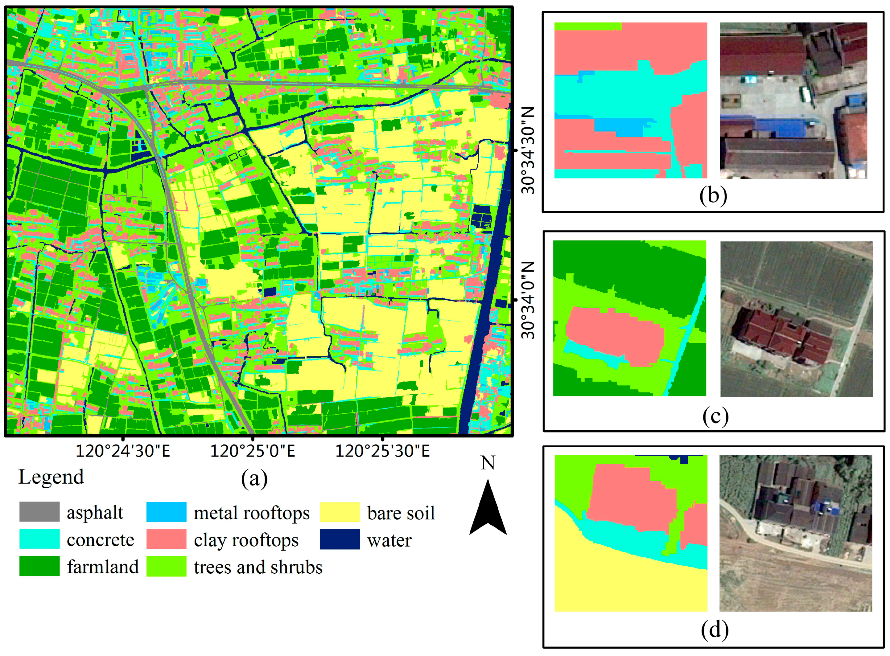
3.1. Stage 1: Mapping Land-Use and Land-Cover (LULC) Using OBIA

In order to ensure the simplicity of the entire distinction process, a single-scale non-hierarchical classification approach was adopted in eCognition® (v9.0, Trimble Germany GmbH, Munich, Germany) in this stage. First, a segmentation algorithm was operated and a set of objects (segments) was generated, which was semantic meaningful. Many papers used multiresolution segmentation embedded in eCognition software package [27,28,29]. Multiresolution segmentation is also known as Fractal Net Evolution Approach (FNEA), which is based on region growing methods and based on some certain homogeneity criteria: scale parameter, shape and compactness [30,31].
Usually, optimum segmentation parameters were obtained by subjective manual trial-and-error test. To make our framework operational and portable, an objective method named Estimation of Scale Parameter, i.e., ESP2 tool [32], was used to identify the statistically most suitable scale parameter for segmentation algorithm. ESP tool iteratively generates image-objects at multiple scale levels in fixed step size and calculates the local variance (LV) in each scale. The rates of change of LV (ROC-LV) were plotted against the corresponding scale in Figure 4. Based on the plot diagram, the peaks of the curve indicated appropriate scale parameter for segmentation [33,34,35]. The scale of 110 appeared promising as the first break in ROC-LV curve after continuous and abrupt decay. Dotted vertical lines indicated optimal scale parameters in Figure 4. As a result, we set segmentation scale as 110.
A visual assessment showed that the ESP2 tool identified the suitable scale parameter accurately to delineate meaningful objects, especially rooftops and concrete materials.
The shape and color parameters were weighted equally as 0.5, whereas the compactness was prioritized instead of smoothness and set as 0.8 because we focus on extracting buildings, especially the rooftops of settlements and industrial area which are more compact spatially.
After creating these objects, support vector machine (SVM) classifier was employed to identify the LULC types [36,37]. An automatic methodology called SEparability and THresholds (SEaTH) [38] tool was adopted in feature selection step to seek significant features of optimal class separation [15,39]. SEaTH calculates the separability in Jeffries–Matusita distance and the corresponding thresholds of object classes for any number of given features on training examples. Eventually, mean values of brightness and all image bands, Normalized Difference Vegetation Index (NDVI), standard deviation, and GLCM (homogeneity, contrast, dissimilarity, entropy, angular second moment, mean, standard deviation and correlation) are selected as optimal feature subset and used in SVM classifier. All these features are normalized before classification applied. An SVM radial basis function (RBF) kernel was applied using the optimal parameters obtained from 5-fold cross-validation in LIBSVM [40].
One thing to note here is that asphalt and water were not treated as automatic classification categories. Instead, we used land-use map from the National Detailed Land-Use Inventory to assign these types directly. For asphalt category, this material is not universal, and there are only two lanes throughout the study area. Thus, it represents only 1% of the total number of objects after segmentation. Meanwhile, water cover surface is often covered by tree canopy, or aquatic plant, resulting in classification confusion with other land-cover types. Similar to asphalt, water surface only contains the linear feature of canal and few ponds in the study site. It is not only time-consuming, but could also cause harmful effect on other terrain categories’ accuracy, for example classify them as asphalt and water cover.

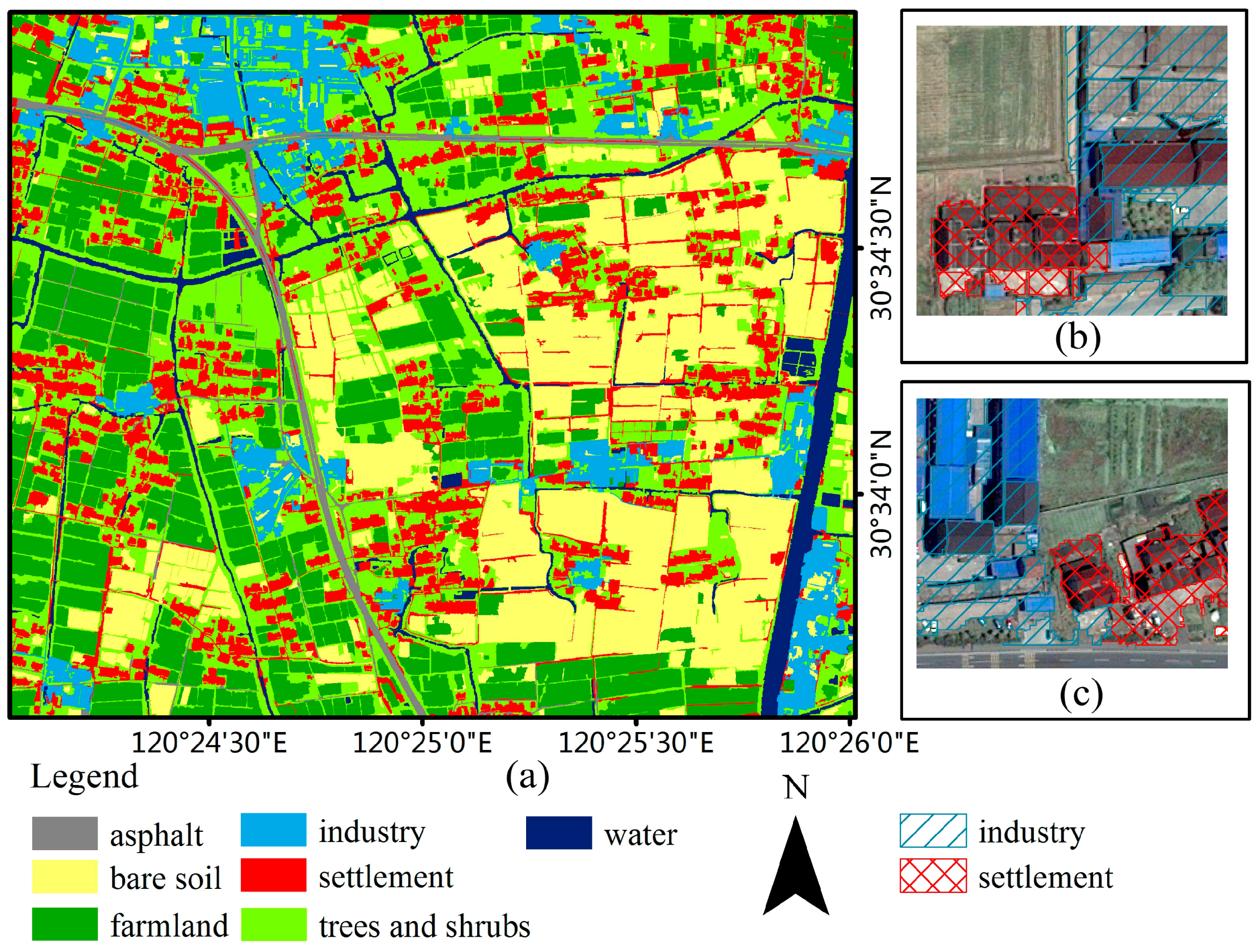
3.2. Stage 2: Landscape Metrics and Chessboard Segmentation

After the Stage 1, the LULC map is derived from Geoeye imagery. However, the area of residential and industrial cover is still unrevealed. In Stage 2, contextual information from inside different land-use units was applied to discriminate settlement and industrial area.
The composition, structure and pattern characteristic of different land-cover objects within a land-use unit, compose valuable information reflecting land use behavior. This information can be described and quantified by landscape metrics.
Defining land-use units is crucial for further landscape patterns analysis. Therefore, a chessboard segmentation was applied to the LULC map derived in Stage 1 to create land-use units, i.e., chessboard square, for further calculating landscape metrics. Chessboard segmentation is a simple segmentation algorithm. It cuts the image into equal square objects of a given size. Block squares (or fishnet squares, or chessboard squares) are commonly used to describe the landscape characteristics of the urban growth [41] and agricultural landscape patterns [42]. Chessboard segmentation can keep the spatial units in a uniform size. In this form, landscape features become comparable among spatial units, i.e., separable or categorizable. It is obvious that chessboard segmentation is a scale-dependent approach. In this paper, we tested different chessboard scales ranging from 40 m to 100 m, with 20 m step-size.
Landscape metrics that characterize area, shape, edge, aggregation and diversity properties were collected as feature space for classification. Percentage of Landscape (PLAND) of each LULC types, Number of Patches (NP), Total Edge (TE), Landscape Shape Index (LSI) and Shannon’s Diversity Index (SHDI) were calculated for each unit and used as features in SVM classifier (Table 1). The RBF kernel was applied again and still using the optimal parameters. Those chessboard squares were classified into three categories: settlement unit, industry unit and other unit. Twenty classification examples for each category are manually selected. Eventually, artificial land-cover types that intersect in settlement unit or industry unit were reclassified into settlement or industry area respectively.

3.3. Top-Down Hierarchical Classification

In order to compare the accuracy of classification, this study also used two other methods to distinguish between these two built-up types. Based on the land-cover map derived from Stage 1, a top-down approach was applied under the results of the first level of classification. Concrete, clay rooftops and metal rooftops were separated into settlement and industry subclasses. Three artificial land-cover types were subdivided into six categories, e.g., settlement clay rooftops and industry clay rooftops. It is noteworthy that there was no new segmentation process in this classification stage, using only the segments generated from Stage 1. Twenty classification examples were equally selected and then the SVM was used to further distinguish settlements and industrial area. More features were added into the classifier. Rooftops and harden ground material in settlements are smaller in objects’ geometry, and also are different in shape. Therefore, geometry metrics containing area, length, width, length/width, asymmetry, border index, compactness, density, roundness, shape index of extend and shape attributes were add into features for classification.

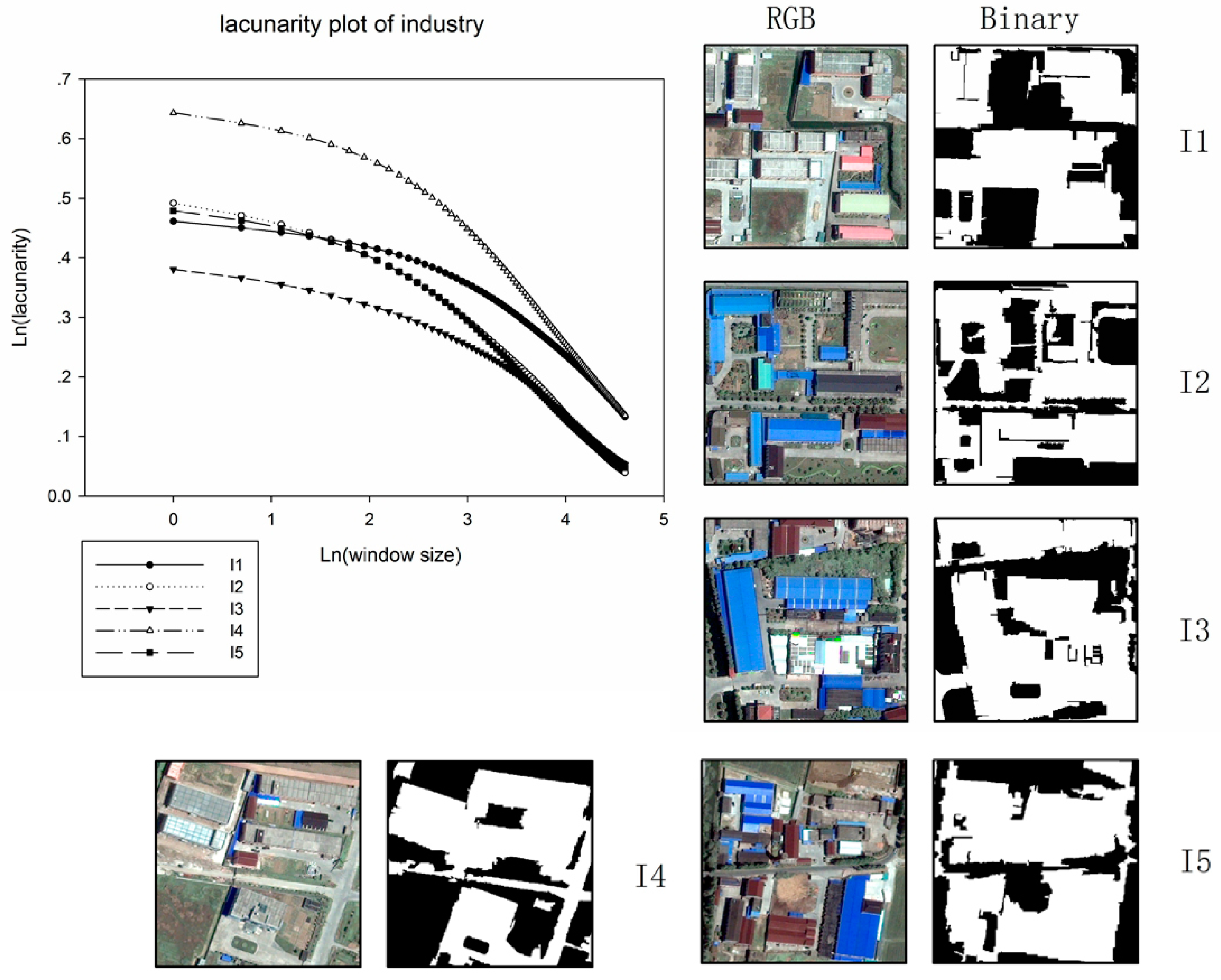
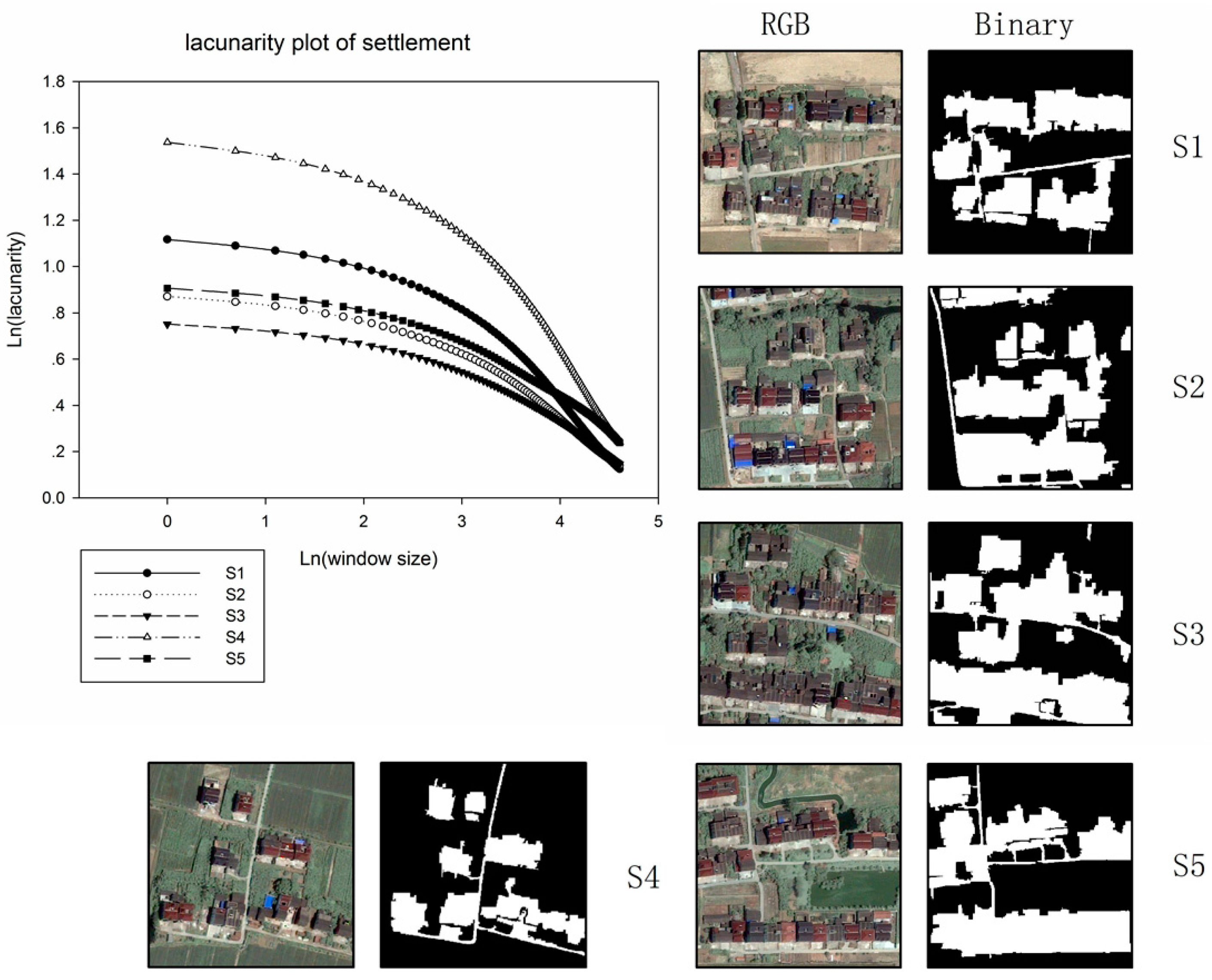
3.4. Lacunarity Based Hierarchical Classification

In addition to the landscape metrics, there are spatial statistics methods to analyze landscape spatial pattern, e.g., the lacunarity. Lacunarity is a measure of “gappiness” or “hole-iness” of a geometric structure and has been used to describe the distribution of the gap sizes in a fractal sequence [43]. Lacunarity algorithm was demonstrated in discriminating land-use types or building types in some urban area [20,21]. In this paper, a lacunarity properties based hierarchical classification was compared with the other two methods. Lacunarity analysis can be based both on binary and grayscale images [44]. Here, we generated build-up areas/non-build-up areas binary images on Stage 1 classification result, and assigned values of 1 or 0, respectively. Lacunarity analysis is carried out in an extension implemented in ArcGIS software [45]. The lacunarity Λ(r) at scale r can be defined as:
Λ ( r ) = S 2 × Q ( S , r ) [ S × Q ( S , r ) ] 2
where S represents occupied sites, and Q ( S , r ) represents the probability of distribution of occupied sites S, which can be obtained by dividing n ( S , r ) by the total number of boxes.
Lacunarity is a function of window size and gliding box, so it is important to identify the optimal size by lacunarity-window size plot. This value can be determined when the image appears as self-autocorrelation. Under these circumstances, three consecutive points on the lacunarity curve are linear, and the coefficient of determination (r2) approaches 1 [43].
The relationship between window-size and lacunarity was analyzed based on 200 m× 200 m examples. Figure 5 illustrated how the lacunarity plots vary with increasing window scale in both settlement and industry area.
Rural settlement area appears as smaller and more scattered patchy built-up areas with larger percent of gaps in analyzed examples than industrial area; meanwhile, gaps in rural settlement area seem more irregular in distribution. Consequently, settlement areas present higher lacunarity than industry areas. As window size increases, the lacunarity values decreased dramatically. For comparison, two types of land-use lacunarity normalized curves were analyzed. In general, land-use features appeared to self-autocorrelate at around 35 window size, implying the quasi-linear decrease in the normalized lacunarity plot. As a result, optimal window size was set as 35. With gliding-box sizes of 3 × 3, 5 × 5, 7 × 7, and 9 × 9, four lacunarity features were calculated for subsequent classification.

3.5. Accuracy Assessment

Accuracy statistics, including producer’s accuracy (PA), user’s accuracy (UA), overall accuracy (OA), and kappa coefficient were calculated based on the error matrix [46]. An error matrix that expresses the number of sample segments assigned to a particular LULC category relative to the actual category is created. The producer’s accuracy is a measure of omission error, indicating the probability of an actual category being correctly classified, whereas the user’s accuracy is a measure of commission error, indicating the probability that a segment classified on the image actually represents that actual category. Overall accuracy is the percentage of correctly classified samples. Kappa analysis is a widely-used and powerful multivariate technique for accuracy assessment. The estimate of kappa is the so-called Kappa coefficient. Kappa coefficient is a measure of overall statistical agreement of a confusion matrix. Therefore, it provides a more rigorous assessment of classification accuracy [47].
In Stage 1, a real land-use and land-cover map was generated through visual interpretation. In visual interpretation step, we used National Detailed Land-Use Inventory Maps in 2011 as reference data (Figure S1). Then, the error matrix was calculated after randomly selected segments were compared with the real land-use and land-cover vector data. In Stage 2, a ground investigation was conducted to confirm that the selected segments are industrial or residential area.
In total, 956 randomly selected segments were used for construction of the error matrix for Stage 1. Among these segments, the man-made objects, i.e., concrete and rooftops, which were classified correctly, were collected to generate error matrix to enable the scale analysis in Stage 2 and the comparison between three different classification approaches. Totally, 467 artificial class objects were collected and no less than 220 objects for settlement and industry types each. A fully rigorous and exhaustive approach named McNemar test was adopted for expressing the statistical significance on different classification results [48]. Z values were calculated on every paired result combinations. A z value matrix clearly identified those classification pairs that are significantly different and those that are not. With four scales of chessboard and two other hierarchy classification approaches, there are a total of 15 z values in the matrix.

4. Results

4.1. Stage 1 Result and Accuracy Assessment

After visual examination on the output maps (Figure 6), land-use and land-cover categories were extracted successfully. The confusion matrix with kappa analysis is shown in Table 2. We found highest Kappa value in clay rooftops of 0.99, and PA of clay rooftops exceeded other LULC accuracies with 99.61%. Both PA and UA of metal rooftops were beyond 90%, with 0.93 Kappa value. For concrete type, PA were 86.82% and UA were 80.58% (Kappa = 0.85). As a result, built-up areas were classified successfully with all PA and UA over 80% and over 0.85 in Kappa per class. We noticed that some bare soil cover in reference were misclassified as concrete, and vice versa, leading to a decrease in both PA of bare soil and UA of concrete. Some trees and shrubs segments were misclassified as clay rooftops too. PA of bare soil and UA of concrete were the two lowest in all classification accuracy results, at 73.81% and 80.58%, respectively, and bare soil and trees and shrubs showed the lowest in Kappa coefficients, 0.71 and 0.81, respectively. The reason is that the spectral characteristics of the bare soil and concrete were similar [49]. Some trees and shrubs segments were misclassified as clay rooftops because of shadow effect located around buildings [50].

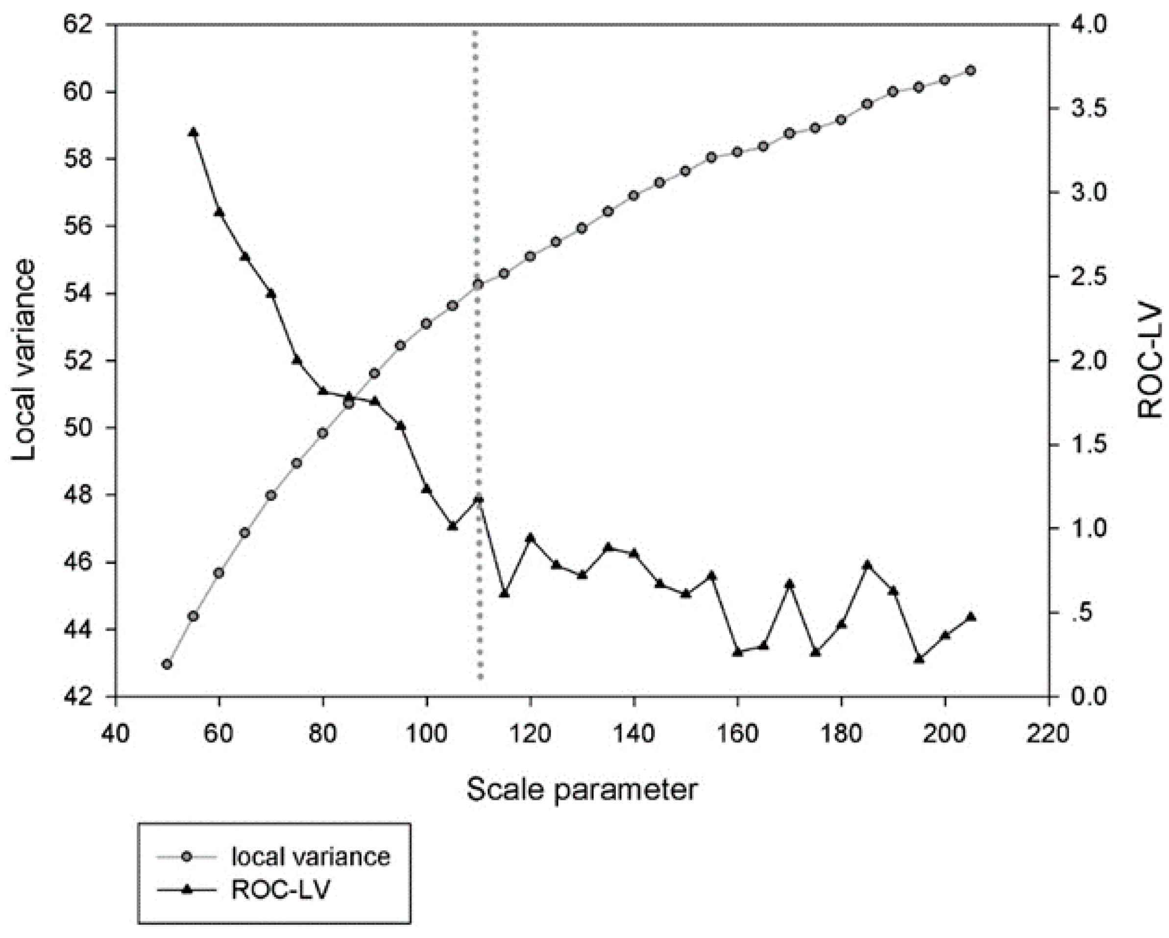
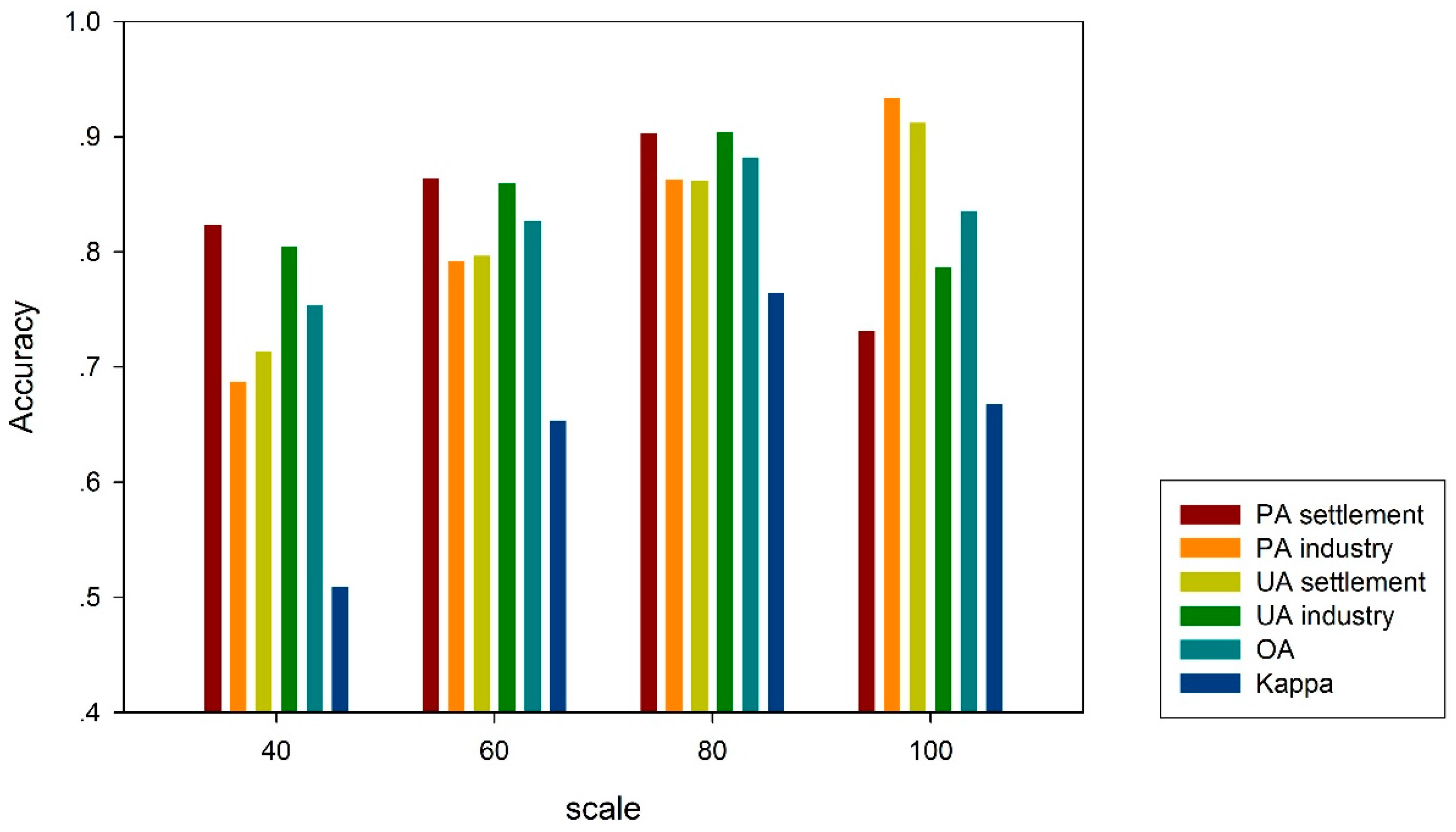
4.2. Landscape Unit Scale Analysis

To analyze scale effect of landscape unit, Table 3 showed the classification accuracies for 40 m, 60 m, 80 m, and 100 m chessboard scales. A histogram of classification accuracies for both types of settlement and industry in all these different scales is provided in Figure 7. This figure presents producer’s accuracy (PA), user’s accuracy (UA), overall accuracies (OA) and kappa coefficient to enable direct assessment of the differences between classification results from individual scale.
With the increasing of scale, both PA of industry and UA of settlement increased continuously, ranging from 68.75% to 93.33% and 71.37% to 91.21%, respectively. In contrast, PA of settlement and UA of industry started to decline after scale 80 m, and overall accuracy and Kappa coefficient followed the same law. Scale 80 m had the highest value in OA and overall Kappa, 88.22% and 0.76, respectively. In general, scale 80 m is a suitable scale to distinguish these two types of land-use in study area. A final classification result of scale 80 m was presented in Figure 8.

4.3. Accuracy Comparison of Three Methods

Classification accuracy results of the other two comparison classification frameworks are shown in Table 4, Results merely using the top-down hierarchical network and lacunarity based hierarchical classification were not satisfactory. Overall accuracy of top-down hierarchical network was 74.73% and overall Kappa value was less than 0.50. Statistics in PA, UA and OA showed the lacunarity based approach produced slightly better classification results than top-down hierarchical network (OA = 75.37%, Kappa = 0.51). Comparing Table 3 with Table 4, it is evident that the approach using landscape metrics by an optimal chessboard scale outperformed the other methods by achieving overall accuracy over 88%.
The McNemar test z values matrix of every classification approach are presented in Table 5, Paired McNemar analysis suggested that using landscape metrics could improve classification accuracy dramatically with appropriate chessboard scales, and the advantage of using lacunarity algorithm was still not significant. The highest value, 5.88, indicated statistically significant different between scale 40 m and 80 m. The value of 5.46 showed significant different between scale 80 m and top-down hierarchical network. There was slight difference between scale 40 m and lacunarity based approach, also observed with similar OA and overall kappa in Table 3 and Table 4.

5. Discussion

5.1. Landscape Unit and Landscape Metrics

Landscape patterns in land-use spatial units can reflect various human land-use behaviors. In this study, the concept of rural residential dwelling unit or housing unit is introduced. A typical rural settlement unit often contains the following features: a house with outbuildings, grain-sunning ground, garden or farmland around the main building. Accordingly, an industry unit contains a larger area of artificial material, i.e., rooftops and concrete, and smaller area of natural surface such as lawn.
The landscape characteristics of rural settlement units show clear differences from those of industry units. The settlement units have diverse land-cover types, while the industry units are generally dominated by artificial material. Consequently, rural settlement units and industry units show significant differences in patch size, patch number, patch edge, fragmentation and diversity. These distinct patterns captured by landscape analysis provide valuable information to improve the discrimination of settlement and industry units in rural region.
Few previous studies focused on the landscape characteristics for classification procedure, although some landscape metrics such as ratio of effective mesh size was proposed and reported to improve the accuracy of object-based classification in a hierarchy approach [19]. However, landscape metrics were not inherent designed for the classification step in image processing, and they are typically used for investigating detailed LULC types in the classification results [23]. In this paper, chessboard segmentation was adopted to generate a set of landscape spatial units, then the landscape metrics was calculated in each spatial units.
This study confirms that landscape properties presented at the chessboard segment squares can provide valuable information in classification. Spectral and textures are the inherent characteristics of the object, and they are not sufficient for classification or discrimination of heterogeneity in complex scenario. Therefore, the contextual information about the relationship between the object and its surrounding features or circumstances is essential. By investigating landscape patterns in residential and industrial units, significant difference was found in proportion of LULC types, patches number, edges and diversity between these two land-use units. Thus, landscape metrics in various segmentation scales were used and can be beneficial for classification. The comparative analysis demonstrates that landscape and chessboard methods outperformed the hierarchical network and lacunarity algorithm in this study.

5.2. Landscape Unit Scale Effect

Chessboard segmentation is a scale-dependent method, and the spatial scale variation affect the accuracy of classification. By using an inapposite scale such as 40 m, a similar unsatisfying result was obtained compared to the other two hierarchy methods (OA = 75.37% in Table 3, OA = 74.73% and 75.37% in Table 4). Beyond the optimal scale 80 m, both overall accuracy and Kappa value started to decrease. Although the OA was still over 80% in an oversize scale, there was no evidence that a larger scale would benefit separation of the industrial and settlement areas. The larger the scale, the more error occurred for the classification of industry area, and substantial confusion is produced between these two types. Meanwhile, the scale 80 m makes practical sense. The building blocks in industry areas approximately occupy 80 × 80 m squares. Thus, the average area of buildings should be calculated as reference before landscape unit scale analysis.
It is crucial to generate a set of spatial units for calculating landscape metrics, because these metrics are designed for characterizing LULC distribution in a certain spatial scale. We chose chessboard segmentation since each segment has a same spatial area. Furthermore, the boundaries of segments from chessboard segmentation does not coincide with the corresponding elements in the landscape, and a patch or a LULC class type may extend beyond the boundary of a segment unit, causing so-called scale problem and boundary problem [51,52]. To address the scale problem, we analyzed the classification accuracy with respect to different chessboard scales ranging from 40 to 100 m, and identified the optimal scale for classification scheme. Unfortunately, the boundary problem caused by fragmentation in patches, classes and landscape is not investigated, as the main purpose of this study is to develope a simple solution for discrimination of settlements and industrial area in rural areas to fulfill the urgent need for the detailed information in rural or agricultural lands.

5.3. Lacunarity Algorithm and Limitation

This study found that there is no significant improvement by only using lacunarity-based hierarchical classification approach for discrimination of dispersed settlements and industrial area in rural region. This is because the lacunarity method only measures the distribution of gap size among land-cover features, which is suitable to distinguish features in state of aggregation, such as broadleaf forest and coniferous forest in tropical forest canopies [43], or aggregated urban structure [20]. On the contrary, the lacunarity algorithm is not appropriate to extract the dispersed industrial spot in rural area, as there is no obvious aggregated pattern in settlement and industrial buildings, neither clear boundaries exist between these two types of LULC. Table 6 summarizes the pros and cons of the classification methods tested in this paper.

5.4. Classification Framework Portability

The simplicity and objectivity of a method is a premise of the feasibility, portability and universality of this method. Various land-cover features have different spatial scales in remotely sensed images, and many articles tend to adopt multi-scale concept and hierarchical classification [32,33,34,35]. However, these classification frameworks often lead to a trial-and-error problem, as a result of the visual assessment of the segmentation suitability [32]. This paper demonstrated a simple and feasible classification procedure in Stage 1 by combining ESP, SEaTH, and LIBSVM tools [53,54], and optimum parameters were obtained by objective statistics. Owing to the universal characteristics, the classification schema in Stage 1 can be also transplant to other classification applications.
The classification framework in Stage 2 highly depends on the spatial scale, so a single parameter is not sufficient when generalized to other datasets or other study sites. However, a specific relationship between the scale parameters and the spatial distribution characteristics of buildings is found in this study. This is in agreement with the study in lacunarity [21], in which the optimum window size was related to the mean building block sizes. However, this relationship still needs to be further validated using independent dataset, and a standard and objective process need to be introduced to determine scale parameter.

5.5. Potential Applications

Previously, some studies were located in slum districts or shantytowns in urban and suburban areas [3,16,20]. Only few studies focused on discrimination of land-use types of rural area or agriculture land. Some articles differentiate LULC types or building types by integrating VHR and normalized Digital Surface Model (nDSM) derived from radar data [21]. However, radar data may meet challenge in coverage of rural area, as the height of factory and settlement buildings are similar, between 3 and 4 floors in typical rural areas of the Yangtze River Delta. Thus, it is necessary to develop some approaches for subdivision of LULC using only VHR multispectral data. Our method is developed based on the orbital VHR data with temporally consistent observation, making it possible to analyze the rural LULC changes.

6. Conclusions

In order to obtain precise information of land-use and discriminate settlements and industrial area in rural areas, this paper demonstrates a classification scheme integrating OBIA, landscape metrics and chessboard segmentation. A LULC map containing land-cover material information was first generated from GeoEye-1 image using traditional OBIA method. Next, a chessboard segmentation and landscape analysis were conducted to capture the contextual information between the object and its surroundings in each unit. The landscape characteristics were further integrated in SVM classification algorithm, and settlements and industry area were successfully distinguished.
Two commonly used approaches, i.e., the top-down hierarchical classification network using spectral, textural and shape properties, and lacunarity based hierarchical classification were also tested in our study. The comparative analysis demonstrates that our method performed better and produced more accurate results than the two other approaches, with the highest overall accuracy, Kappa coefficient and McNemar test. Thus, the landscape properties can contribute to the discrimination of settlement and industry area in complex scenarios.
Furthermore, the scale dependence of our method was also tested by analyzing the classification accuracy at various scales, i.e., 40 m, 60 m, 80 m, and 100 m. The overall accuracy ranged from 75% to 88%, and Kappa coefficient ranged from 0.51 to 0.76, both peaking at scale 80 m. The optimal scale parameter was found to be related to the size of the building blocks in industry area.

Supplementary Materials

The following are available online at www.mdpi.com/2072-4292/8/10/845/s1, Figure S1. Example (a,b) are Geoeye images overlaid by reference data, example (c,d) are land-use and land-cover maps from Stage 1. Example (a,c) provide a comparison from a same location, accordingly (b,d) are also from the same location. The Geoeye images (a,b) are overlaid by Land-Use Inventory Maps, which are blue vector data with land-use attributes. Visual interpretation was conducted by using Geoeye imagery and this vector data as reference. The real land-use and land-cover map was generated in visual interpretation workspace.

Acknowledgments

This research was supported by International Science & Technology Cooperation Program of China (2012DFA20930). We also thank the anonymous reviewers for their constructive comments.

Author Contributions

Xinyu Zheng designed the study and wrote the manuscript; Muye Gan and Jing Zhang supervised the study and reviewed the manuscript; Yang Wang, Ke Wang, Zhangquan Shen and Ling Zhang contributed to the discussions; and Longmei Teng contributed to the discussions and revise writing. All authors read and approved the final manuscript.

Conflicts of Interest

The authors declare no conflict of interest.

References

  1. Hansen, M.C.; DeFries, R.S.; Townshend, J.R.; Sohlberg, R. Global land cover classification at 1 km spatial resolution using a classification tree approach. Int. J. Remote Sens. 2000, 21, 1331–1364. [Google Scholar] [CrossRef]
  2. Jensen, J.R. Digital Change Detection. In Introductory Digital Image Processing: A Remote Sensing Perspective, 3rd ed.; University of South Carolina: Columbus, OH, USA, 1986; pp. 337–339. [Google Scholar]
  3. Owen, K.K.; Wong, D.W. Exploring structural differences between rural and urban informal settlements from imagery: The basureros of Cobán. Geocarto Int. 2013, 28, 562–581. [Google Scholar] [CrossRef]
  4. Tuia, D.; Ratle, F.; Pacifici, F.; Kanevski, M.F.; Emery, W.J. Active learning methods for remote sensing image classification. IEEE Trans. Geosci. Remote Sens. 2009, 47, 2218–2232. [Google Scholar] [CrossRef]
  5. Hussain, M.; Chen, D.; Cheng, A.; Wei, H.; Stanley, D. Change detection from remotely sensed images: From pixel-based to object-based approaches. ISPRS J. Photogramm. 2013, 80, 91–106. [Google Scholar] [CrossRef]
  6. Nagendra, H.; Lucas, R.; Honrado, J.P.; Jongman, R.H.G.; Tarantino, C.; Adamo, M.; Mairota, P. Remote sensing for conservation monitoring: Assessing protected areas, habitat extent, habitat condition, species diversity, and threats. Ecol. Indic. 2013, 33, 45–59. [Google Scholar] [CrossRef]
  7. Kuffer, M.; Barrosb, J. Urban morphology of unplanned settlements: The use of spatial metrics in VHR remotely sensed images. Procedia Environ. Sci. 2011, 7, 152–157. [Google Scholar] [CrossRef]
  8. Li, X.; Chen, W.; Cheng, X.; Wang, L. A comparison of machine learning algorithms for mapping of complex surface-mined and agricultural landscapes using ZiYuan-3 stereo satellite imagery. Remote Sens. 2016, 8, 514. [Google Scholar] [CrossRef]
  9. Blaschke, T. Object based image analysis for remote sensing. ISPRS J. Photogramm. Remote Sen. 2010, 65, 2–16. [Google Scholar] [CrossRef]
  10. Nussbaum, S.; Menz, G. Satellite Imagery and Methods of Remote Sensing. In Object-Based Image Analysis and Treaty Verification: New Approaches in Remote Sensing-Applied to Nuclear Facilities in Iran; Springer Science & Business Media: Berlin, Germany, 2008; pp. 17–27. [Google Scholar]
  11. Su, W.; Li, J.; Chen, Y.; Liu, Z.; Zhang, J.; Low, T.M.; Suppiah, I.; Hashim, S.A.M. Textural and local spatial statistics for the object-oriented classification of urban areas using high resolution imagery. Int. J. Remote Sens. 2008, 29, 3105–3117. [Google Scholar] [CrossRef]
  12. Pacifici, F.; Chini, M.; Emery, W.J. A neural network approach using multi-scale textural metrics from very high-resolution panchromatic imagery for urban land-use classification. Remote Sens. Environ. 2009, 113, 1276–1292. [Google Scholar] [CrossRef]
  13. Zhang, R.; Zhu, D. Study of land cover classification based on knowledge rules using high-resolution remote sensing images. Expert Syst. Appl. 2011, 38, 3647–3652. [Google Scholar] [CrossRef]
  14. Han, N.; Du, H.; Zhou, G.; Sun, X.; Ge, H.; Xu, X. Object-based classification using SPOT-5 imagery for Moso bamboo forest mapping. Int. J. Remote Sens. 2014, 35, 1126–1142. [Google Scholar] [CrossRef]
  15. Niebergall, S.; Loew, A.; Mauser, W. Integrative assessment of informal settlements using VHR remote sensing data—The Delhi case study. IEEE J. Sel. Top. Appl. Earth Obs. Remote Sens. 2008, 1, 193–205. [Google Scholar] [CrossRef]
  16. Kuffer, M.; Barros, J.; Sliuzas, R.V. The development of a morphological unplanned settlement index using very-high-resolution (VHR) imagery. Comput. Environ. Urban Syst. 2014, 48, 138–152. [Google Scholar] [CrossRef]
  17. Chen, G.; Liang, S.; Chen, J. The extraction of plantation with texture feature in high resolution remote sensing image. In Proceedings of the 3rd International Workshop on Earth Observation and Remote Sensing Applications, Changsha, China, 11–14 June 2014; pp. 384–387.
  18. Han, N.; Du, H.; Zhou, G.; Xu, X.; Ge, H.; Liu, L.; Gao, G.; Sun, S. Exploring the synergistic use of multi-scale image object metrics for land-use/land-cover mapping using an object-based approach. Int. J. Remote Sens. 2015, 36, 3544–3562. [Google Scholar] [CrossRef]
  19. Han, N.; Wang, K.; Yu, L.; Zhang, X. Integration of texture and landscape features into object-based classification for delineating Torreya using IKONOS imagery. Int. J. Remote Sens. 2012, 33, 2003–2033. [Google Scholar] [CrossRef]
  20. Kit, O.; Lüdeke, M.; Reckien, D. Texture-based identification of urban slums in Hyderabad, India using remote sensing data. Appl. Geogr. 2012, 32, 660–667. [Google Scholar] [CrossRef]
  21. Ma, L. Discrimination of residential and industrial buildings using LiDAR data and an effective spatial-neighbor algorithm in a typical urban industrial park. Eur. J. Remote Sens. 2015, 48, 1–15. [Google Scholar] [CrossRef]
  22. Fan, C.; Myint, S. A comparison of spatial autocorrelation indices and landscape metrics in measuring urban landscape fragmentation. Landsc. Urban Plan 2014, 121, 117–128. [Google Scholar] [CrossRef]
  23. McGarigal, K.; Cushman, S.A.; Neel, M.C.; Ene, E. FRAGSTATS: Spatial Pattern Analysis Program for Categorical Maps. Available online: http://www.umass.edu/landeco/research/fragstats/fragstats.html (accessed on 10 May 2016).
  24. Turner, M.G.; Gardner, R.H.; O’Neill, R.V. Landscape Ecology in Theory and Practice; Springer: New York, NY, USA, 2015; pp. 479–494. [Google Scholar]
  25. Jaeger, J.A.G. Landscape division, splitting index, and effective mesh size: New measures of landscape fragmentation. Landsc. Ecol. 2000, 15, 115–130. [Google Scholar] [CrossRef]
  26. Statistics Bureau of Tongxiang. Tongxiang Statistical Year Books; China Statistical Press: Beijing, China, 2012. [Google Scholar]
  27. Blaschke, T.; Hay, G.J.; Kelly, M.; Lang, S.; Hofmann, P.; Addink, E.; Feitosa, R.Q.; van der Meer, F.; van der Werff, H.; van Coillie, F.; et al. Geographic object-based image analysis—Towards a new paradigm. ISPRS J. Photogramm. 2014, 87, 180–191. [Google Scholar] [CrossRef] [PubMed]
  28. Yu, Q.; Gong, P.; Clinton, N.; Biging, G.; Kelly, M.; Schirokauer, D. Object-based detailed vegetation classification with airborne high spatial resolution remote sensing imagery. Photogramm. Eng. Remote Sens. 2006, 72, 799–811. [Google Scholar] [CrossRef]
  29. Bhaskaran, S.; Paramananda, S.; Ramnarayan, M. Per-pixel and object-oriented classification methods for mapping urban features using IKONOS satellite data. Appl. Geogr. 2010, 30, 650–665. [Google Scholar] [CrossRef]
  30. Baatz, M.; Schäpe, A. Multiresolution segmentation: An optimization approach for high quality multi-scale image segmentation. Angew. Geogr. Inf. Verarb. 2000, 58, 12–23. [Google Scholar]
  31. Benz, U.C.; Hofmann, P.; Willhauck, G.; Lingenfelder, I.; Heynen, M. Multi-resolution, object-oriented fuzzy analysis of remote sensing data for GIS-ready information. ISPRS J. Photogramm. Remote Sen. 2004, 58, 239–258. [Google Scholar] [CrossRef]
  32. Drăguţ, L.; Csillik, O.; Eisank, C.; Tiede, D. Automated parameterisation for multi-scale image segmentation on multiple layers. ISPRS J. Photogramm. Remote Sen. 2014, 88, 119–127. [Google Scholar] [CrossRef] [PubMed]
  33. Drǎguţ, L.; Tiede, D.; Levick, S.R. ESP: A tool to estimate scale parameter for multiresolution image segmentation of remotely sensed data. Int. J. Geogr. Inf. Sci. 2010, 24, 859–871. [Google Scholar] [CrossRef]
  34. Hellesen, T.; Matikainen, L. An Object-based approach for mapping shrub and tree cover on grassland habitats by use of LiDAR and CIR orthoimages. Remote Sens. 2013, 5, 558–583. [Google Scholar] [CrossRef]
  35. Belgiu, M.; Drǎguţ, L. Comparing supervised and unsupervised multiresolution segmentation approaches for extracting buildings from very high resolution imagery. ISPRS J. Photogramm. Remote Sen. 2014, 96, 67–75. [Google Scholar] [CrossRef] [PubMed]
  36. Mountrakis, G.; Im, J.; Ogole, C. Support vector machines in remote sensing: A review. ISPRS J. Photogramm. 2011, 66, 247–259. [Google Scholar] [CrossRef]
  37. Heumann, B.W. An object-based classification of mangroves using a hybrid decision tree—Support vector machine approach. Remote Sens. 2011, 3, 2440–2460. [Google Scholar] [CrossRef]
  38. Nussbaum, S.; Niemeyer, I.; Canty, M.J. SEATH—A new tool for automated feature extraction in the context of object-based image analysis. In Proceedings of the 1st International Conference on Object-Based Image Analysis, Salzburg, Austria, 4–5 July 2006.
  39. Gao, Y.; Marpu, P.; Niemeyer, I.; Runfola, D.M.; Giner, N.M.; Hamill, T.; Pontius, R.G. Object-based classification with features extracted by a semi-automatic feature extraction algorithm—SEaTH. Geocarto Int. 2011, 26, 211–226. [Google Scholar] [CrossRef]
  40. Fan, R.; Chen, P.; Lin, C. Working set selection using second order information for training support vector machines. J. Mach. Learn. Res. 2005, 6, 1889–1918. [Google Scholar]
  41. Zhang, Z.; Su, S.; Xiao, R.; Jiang, D.; Wu, J. Identifying determinants of urban growth from a multi-scale perspective: A case study of the urban agglomeration around Hangzhou Bay, China. Appl. Geogr. 2013, 45, 193–202. [Google Scholar] [CrossRef]
  42. Su, S.; Xiao, R.; Zhang, Y. Multi-scale analysis of spatially varying relationships between agricultural landscape patterns and urbanization using geographically weighted regression. Appl. Geogr. 2012, 32, 360–375. [Google Scholar] [CrossRef]
  43. Malhi, Y.; Román-Cuesta, R.M. Analysis of lacunarity and scales of spatial homogeneity in IKONOS images of Amazonian tropical forest canopies. Remote Sens. Environ. 2008, 112, 2074–2087. [Google Scholar] [CrossRef]
  44. Dong, P. Test of a new lacunarity estimation method for image texture analysis. Int. J. Remote Sens. 2000, 21, 3369–3373. [Google Scholar] [CrossRef]
  45. Dong, P. Lacunarity analysis of raster datasets and 1D, 2D, and 3D point patterns. Comput. Geosci. 2009, 35, 2100–2110. [Google Scholar] [CrossRef]
  46. Congalton, R.G. A review of assessing the accuracy of classifications of remotely sensed data. Remote Sens. Environ. 1991, 37, 35–46. [Google Scholar] [CrossRef]
  47. Thapa, R.B.; Murayama, Y. Urban mapping, accuracy, & image classification: A comparison of multiple approaches in Tsukuba City, Japan. Appl. Geogr. 2009, 29, 135–144. [Google Scholar] [Green Version]
  48. Foody, G.M. Thematic map comparison: Evaluating the statistical significance of differences in classification accuracy. Photogramm. Eng. Remote Sens. 2004, 70, 627–633. [Google Scholar] [CrossRef]
  49. Weng, Q. Remote sensing of impervious surfaces in the urban areas: Requirements, methods, and trends. Remote Sens. Environ. 2012, 117, 34–49. [Google Scholar] [CrossRef]
  50. Sawaya, K. Extending satellite remote sensing to local scales: Land and water resource monitoring using high-resolution imagery. Remote Sens. Environ. 2003, 88, 144–156. [Google Scholar] [CrossRef]
  51. Moser, B.; Jaeger, J.A.G.; Tappeiner, U.; Tasser, E.; Eiselt, B. Modification of the effective mesh size for measuring landscape fragmentation to solve the boundary problem. Landsc. Ecol. 2007, 22, 447–459. [Google Scholar] [CrossRef]
  52. Girvetz, E.H.; Thorne, J.H.; Berry, A.M.; Jaeger, J.A.G. Integration of landscape fragmentation analysis into regional planning: A statewide multi-scale case study from California, USA. Landsc. Urban Plan 2008, 86, 205–218. [Google Scholar] [CrossRef]
  53. Lausch, A.; Salbach, C.; Schmidt, A.; Doktor, D.; Merbach, I.; Pause, M. Deriving phenology of barley with imaging hyperspectral remote sensing. Ecol. Model. 2015, 295, 123–135. [Google Scholar] [CrossRef]
  54. Chang, C.; Lin, C. LIBSVM: A library for support vector machines. Acm Trans. Intell. Syst. Technol. 2011, 2, 1–27. [Google Scholar] [CrossRef]
Figure 1. Study area location in a rural region of Zhejiang, and a Geoeye image in true color.
Remotesensing 08 00845 g001
Figure 2. Example of artificial cover types: (a) Clay rooftops and grain-sunning ground of settlement; (b) Clay rooftops of industry; (c) Metal rooftops of factory; (d) Metal rooftops of settlement; and (e) Concrete rooftops and roads in factory.
Remotesensing 08 00845 g002
Figure 3. Flow chart of the classification network in this paper, including Stage 1, Stage 2 and the comparison methods.
Remotesensing 08 00845 g003
Figure 4. Plot diagram of local variance (LV, black circles and gray line) and rates of change of LV (ROC-LV, black triangles and black line) plotted against corresponding scale. Grey dotted vertical lines indicated optimal scale parameters selected.
Remotesensing 08 00845 g004
Figure 5. Ln(lacunarity) plotted against ln(window size), and industrial and residential samples are analyzed (samples are 200 m× 200 m). I and R represent industrial and residential, respectively. The x- and y-axes represent the moving window size and lacunarity value, respectively, all in logarithmic scale. This means the width of moving window square in pixels and lacunarity values were logarithmically transformed. If the decline in log-log lacunarity curve is linear (or quasi-linear) over a range of spatial scale, then the image exhibits self-similar or fractal properties over that range of scales.
Remotesensing 08 00845 g005aRemotesensing 08 00845 g005b
Figure 6. Output map from SVM classifier in Stage 1, for the whole study area (a); some subset example for industry area (b); settlement surround by agriculture land (c); and settlement surround by uncultivated land (d).
Remotesensing 08 00845 g006
Figure 7. A summary histogram of producer’s accuracy (PA), user’s accuracy (UA), and overall accuracies (OA) for 40 m, 60 m, 80 m, and 100 m chessboard scales.
Remotesensing 08 00845 g007
Figure 8. Final classification map for the whole study area (a) at scale 80 m, and some subset example presented the mix situation that there are no clear boundaries between industry and settlement area, and the approach proposed discriminated this two area successfully (b,c).
Remotesensing 08 00845 g008
Table 1. Description of object features selected in classification network.
Classification StageObject FeaturesDescription
Mapping land-use and land-cover in Stage 1Mean brightness Mean layer 1 to 4Mean values of brightness and all image bands
Stdev layer 1 to 4Standard deviation for each object in all bands
NDVIMean values for each object in Normalized Difference Vegetation Index
GLCM_homogeneity, GLCM_contrast, GLCM_dissimilarity, GLCM_entropy, GLCM_Ang.2nd moment, GLCM_mean, GLCM_standard deviation, GLCM_correlationEight grey-level co-occurrence matrix (GLCM) texture measures calculated for each object, from each image layer values
Top-down hierarchical classificationExcept object features in Stage 1, add: Area, length, width, length/width, asymmetry, border index, compactness, density, roundness, shape indexExtent and shape attributes of each object
Lacunarity based hierarchical classificationExcept object features in Stage 1, add lacunarity images window size: 35 3 × 3, 5 × 5, 7 × 7, 9 × 9Lacunarity analyze result from binary image with moving-window size of 35 pixel, and gliding-box size of 3 × 3, 5 × 5, 7 × 7, 9 × 9
Landscape metrics and chessboard segmentation methodPLAND_asphalt, PLAND_concrete, PLAND_farmland, PLAND_clay rooftops, PLAND_metal rooftops, PLAND_trees and shrubs, PLAND_bare soil, PLAND_water, NP, TE, LSI, SHDIPercentage of Landscape (PLAND) of each LULC type in each square and Number of Patches (NP), Total Edge (TE), Landscape Shape Index (LSI) and Shannon’s Diversity Index (SHDI) in landscape metrics
Table 2. Error matrix for the object-based image analysis (OBIA) classification result in Stage 1. PA: producer’s accuracy; UA: user’s accuracy; OA: overall accuracy.
Reference Class
ConcreteMetal RooftopsClay RooftopsFarmlandTrees and ShrubsBare SoilSum
Predicted classconcrete112211419139
metal rooftops2990010102
clay rooftops442563263296
farmland01010918119
trees and shrubs000101833196
bare soil11000093104
Sum129106257123215126
PA86.82%93.40%99.61%88.62%85.12%73.81%
UA80.58%97.06%86.49%91.60%93.37%89.42%
Kappa Per Class85%93%99%87%81%71%
OA89.12%
Overall Kappa87%
Table 3. A summary of classification accuracies for different chessboard scales.
Scale 40 mReference Class Scale 60 mReference Class
SettlementIndustrySumSettlementIndustrySum
Predicted classSettlement18775262Settlement19650246
Industry40165205industry31190221
Sum227240 Sum227240
PA82.38%68.75% PA86.34%79.17%
UA71.37%80.49% UA79.67%85.97%
OA75.37% OA82.66%
Kappa51% Kappa65%
Scale 80 mReference Class Scale 100 mReference Class
SettlementIndustrySumSettlementIndustrySum
Predicted classsettlement20533238settlement16616182
industry22207229industry61224285
Sum227240 Sum227240
PA90.31%86.25% PA73.13%93.33%
UA86.13%90.39% UA91.21%78.60%
OA88.22% OA83.51%
Kappa76% Kappa67%
Table 4. A summary of results from comparison classification frameworks.
Hierarchy NetworkReference Class Lacunarity ApproachReference Class
SettlementIndustrySumSettlementIndustrySum
Predicted classsettlement16354217settlement16452216
industry64186250industry63188251
Sum227240 Sum227240
PA71.81%77.50% PA72.25%78.33%
UA75.12%74.40% UA75.93%74.90%
OA74.73% OA75.37%
Kappa49% Kappa51%
Table 5. McNemar test matrix showing the statistical significance between classification approaches.
ScalesHierarchy NetworkLacunarity
40 m60 m80 m100 m
Scales40 m
60 m3.47 **
80 m5.88 **3.06 **
100 m3.1 **0.372.37 *
Hierarchy Network0.233.03 **5.46 **3.36 **
Lacunarity0.082.81 **5.35 **3.21 **0.65
Where z values ≥2.57 (**) are statistically significant at the 99% confidence; Z values ≥1.96 (*) are statistically significant at the 95% confidence.
Table 6. A summary of the pros and cons of the classification methods tested.
Classification MethodsAdvantagesLimitations
Landscape metrics and chessboard segmentation methodTaking the differences in landscape properties between LULC types into consideration, successfully discriminated land-use typesTime consuming, still room for improvement
Top-down hierarchical classificationEasy to deployCauses confusion, spectral and textural information is not enough for classification heterogeneity due to the similarity between different LULC types.
Lacunarity based hierarchical classificationSuitable for discrimination of forest types and urban structure in aggregated formInappropriate in extraction of dispersed and disorderly target

