A High-Fidelity Haze Removal Method Based on HOT for Visible Remote Sensing Images

Abstract

Spatially varying haze is a common feature of most satellite images currently used for land cover classification and mapping and can significantly affect image quality. In this paper, we present a high-fidelity haze removal method based on Haze Optimized Transformation (HOT), comprising of three steps: semi-automatic HOT transform, HOT perfection and percentile based dark object subtraction (DOS). Since digital numbers (DNs) of band red and blue are highly correlated in clear sky, the R-squared criterion is utilized to search the relative clearest regions of the whole scene automatically. After HOT transform, spurious HOT responses are first masked out and filled by means of four-direction scan and dynamic interpolation, and then homomorphic filter is performed to compensate for loss of HOT of masked-out regions with large areas. To avoid patches and halo artifacts, a procedure called percentile DOS is implemented to eliminate the influence of haze. Scenes including various land cover types are selected to validate the proposed method, and a comparison analysis with HOT and Background Suppressed Haze Thickness Index (BSHTI) is performed. Three quality assessment indicators are selected to evaluate the haze removed effect on image quality from different perspective and band profiles are utilized to analyze the spectral consistency. Experiment results verify the effectiveness of the proposed method for haze removal and the superiority of it in preserving the natural color of object itself, enhancing local contrast, and maintaining structural information of original image.

1. Introduction

In recent years, an increasing number of projects and applications are carried out relying on moderate or high-resolution satellite images. Given the constraints of satellite orbital characteristics and atmospheric conditions, comprehensive satellite data with haze-affected scenes are usually obtained. Due to the existence of haze, the image is degraded by the scattering of atmosphere more or less, resulting in reduction of contrast and difficulty in identifying object features [1,2,3]. As a consequence, haze removal from satellite images would normally be treated as a pre-processing step for ground information extraction [4,5].

Theoretically, it is feasible to remove haze from hazy images via atmospheric correction techniques, of which the desirable characteristics should involve robustness (i.e., applicable to a wide range of haze conditions), ease-to-use (i.e., minimal and simple operator) and scene-based since there typically is paucity of ancillary data [5].

Liang et al. [6,7] proposed a cluster matching technique for Landsat TM data based on an assumption that each land cover cluster has the same visible reflectance in both clear and hazy regions. The demand for existence of aerosol transparent bands makes it impractical for high-resolution satellite imagery, since visible bands and the near-infrared band are contaminated by haze more or less. It was noted that haze seems to be a major contributor to the fourth component of tasseled-cap (TC) transformation [8,9]. However, the applicability of the method based on TC transformation is problematic due to the sensitivity to certain ground targets and the necessity to properly scale the estimated haze values.

Zhang et al. [10] proposed a haze optimized transformation (HOT) method for haze evaluation, assuming that digital numbers (DNs) of band red and blue will be highly correlated for pixels within the clearest portions of a scene and that this relationship holds for all surface classes. HOT combined with dark object subtraction (DOS) [11] has been shown to be an operational technique for haze removal of Landsat TM and high-resolution satellite data [10,12]. Although this technique provides good results for vegetated areas, some surface classes (water bodies, snow cover, bare soil and urban targets) can induce low or high HOT values that eventually result in under-correction or over-correction of these targets [10,13]. Liu et al. [14] developed a technique to remove spatially varying haze contamination, comprising three steps: haze detection, haze perfection, and haze removal. This method uses background suppressed haze thickness index (BSHTI) to detect relative haze thickness and virtual cloud point (VCP) for haze removal. Artificial intervention is necessary to outline thick haze and clear regions and set parameters during subsequent processing [14,15]. It is stressed that the two methods are relative atmospheric correction techniques in view of the fact that most image classification algorithms (e.g., unsupervised clustering and supervised maximum likelihood classification) do not require absolute radiometric calibration.

Makarau et al. [16] presented a haze removal method that calculates a haze thickness map (HTM) based on a local non-overlapping search of dark objects. Assuming an additive model of the haze influence, the haze-free signal at the sensor is restored by subtracting the HTM from the hazy images. Makarau et al. [17] continue to develop a novel combined haze/cirrus removal that uses visible bands and a cirrus band to calculate the HTM in [17]. This method is fast and parameter-free since it is independent of critical and time-consuming cirrus parameter estimation. Shen et al. [18] developed a simple but highly efficient and effective method based on the homomorphic filter (HF) [19] for the removal of thin clouds in visible remote sensing images. Three stages are included in this method: cut-off frequency decision, thin cloud removal, and the mosaicking of the cloudy and cloud-free sub-images.

He et al. [20] observed that in most of the non-sky patches of haze-free outdoor images, at least one color channel has very low intensity at some pixels. They proposed an efficient haze removal and depth map estimation method for outdoor colored RGB images based on dark channel prior calculation. Dark channel prior was applied for haze removal of remote sensing image in [21]. Instead of soft matting method, Long et al. [21] refined the atmospheric veil with a low-pass Gaussian filter. In order to eliminate the color distortion and oversaturated areas in the restored images, the transmission is recomputed, which can lead to good results and sufficient speed.

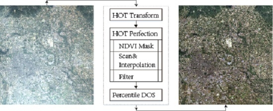
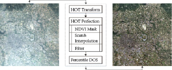
In this paper, we present an effective method based on the HOT transformation for haze or thin clouds removal in visible remote sensing images. We intend to gain a high-fidelity haze-free image especially in RGB channels for the sake of visual recognition and land cover classification. Our proposed method is comprised of three steps in sequence: semi-automatic HOT transform, HOT perfection and percentile DOS with detailed description in the following sections. To verify the effectiveness of our proposed method, experiments on Landsat 8 OLI and Gaofen-2 High-Resolution Imaging Satellite (GF-2) images are carried out. The dehazed results are compared with those of original HOT and BSHTI. Meanwhile, three quality assessment indicators are selected to evaluate the image quality of haze removed results from various perspectives and band profiles are utilized to analyze the spectral consistency. The conclusion is given at the end of this paper.

2. Proposed Method

Through MODTRAN simulations, Zhang et al. [10] found out that DNs of band red and blue are highly correlated in clear sky or thin cloud conditions for Landsat TM data. In the two-dimensional spectral space consisting of band red and blue, a clear line (CL) can be defined, whose direction depends on the characteristics of the scene. The distance of a given pixel from the CL is proportional to the amount of haze that characterizes the pixel, thus making it possible to estimate the haze component to subtract from the original data. The direction of the CL can be expressed by its slope angle θ, and hence HOT, the transformation that quantifies the perpendicular displacement of a pixel from this line can be given by Equation (1):

$$HOT=B_1\text{ sin }\theta -B_3\text{ cos }\theta$$

(1)

where B₁ and B₃ are the pixel’s DNs of band blue and red, respectively.

Equation (1) is derived from a CL through the origin supposing an ideal atmosphere without background aerosols. If the scattering effect of the background aerosols is taken into consideration, the position of the CL would shift, but its slope would not change appreciably since the background aerosol effect is linearly related to other path scattering effects.

Zhang et al. [10] illustrated that diverse atmospheric conditions could be detected in detail by HOT. Nevertheless, some surface types could potentially trigger spurious HOT responses. These classes include snow cover, shadows over snow, water bodies and bare soil. Moro and Halounova [12] confirmed that man-made features could also induce wrong HOT response. These types are called sensitive targets hereafter. The sensibility of HOT response can lead to over-correction or under-correction of sensitive targets and color distortion in RGB synthetic image of haze removal results.

To overcome the shortcomings of original HOT method, a high-fidelity haze removal method based on HOT is proposed and described in next section. It should be noted that haze here means contamination by spatially varying, semitransparent cloud and aerosol layers, which can arise from a variety of atmospheric constituents including water droplets, ice crystals or fog/smog particles [10]. Three stages are included: semi-automatic HOT transform, HOT perfection and percentile DOS. In the first stage, the relative clearest regions of the whole scene are located automatically through R-squared criterion. In the second stage, spurious HOT responses are first masked out and filled by means of four-direction scan and dynamic interpolation, and then homomorphic filter is performed to compensate for loss of HOT of masked-out regions with large areas. Finally, a procedure similar to DOS is implemented to eliminate the influence of haze. In this stage, each band of original images is sliced into different layers according to different HOT response and percentiles of histograms are utilized to determine the adjusted DNs of each layer.

2.1. Semi-Automatic HOT Transform

In order to generate the HOT map of the whole scene, the clearest portions of a scene must be delineated beforehand. As mentioned before, the clearest regions should at least meet the following two conditions:

Condition one (C1): Have relative lower radiances of visible bands.

Condition two (C2): Band blue and red radiances are highly correlated.

The two conditions are useful for us to identify the clearest regions. Thus, we use a non-overlapping window scanning the original image to search regions where the two conditions are met at the same time. We can simply use 64 (0.25 × 256) as a threshold of C1 after stretching the range of radiance to 0–255. As for C2, R-squared is used to measure how well a regression line approximates band radiances of pixels within each window. Generally, an R-squared of 1.0 (100%) indicates a perfect fit. The formula for R-squared is:

$$\mathrm{R}(\mathbf{X},\mathbf{Y})=\text{Cov}(\mathbf{X},\mathbf{Y})/\left[\text{StdDev}\right(\mathbf{X})\times \text{StdDev}(\mathbf{Y}\left)\right]$$

(2)

where X and Y are two vectors representing band blue and red, respectively; and Cov and StdDev are shorthand of covariance and standard deviation, respectively. We choose 0.95 as the threshold of C2. Those windows whose R-squared values are greater than 0.95 and means of visible bands are lower than 64 are stored for a more accurate estimation of the slope of CL. The size of the window should be adjusted according to the real distribution of haze and clouds. By the experimental analysis, it is suggested that the minimum window size had better ensure a field size of 3 km × 3 km. For each stored window, the regression coefficient k is calculated as Equation (3):

$$\mathrm{k}=\frac{n{\displaystyle \sum _{i=1}^n{x}_i{y}_i}-{\displaystyle \sum _{i=1}^n{x}_i}{\displaystyle \sum _{i=1}^n{y}_i}}{n{\displaystyle \sum _{i=1}^n{x_i}^2}-{({\displaystyle \sum _{i=1}^n{x}_i{y}_i})}^2}$$

(3)

where n is the total number of pixels in each window; and x_i and y_i are radiances of band blue and red, respectively. All regression coefficients of stored windows can be represented by a vector K.

Ideally, the clearest regions should contain dense vegetation to reduce impact of sensitive targets. However, there can be cloudless and homogeneous regions with large areas in a scene, whose R-squared values may also greater than 0.95 but regression coefficients are not consistent with dense vegetation regions. Typical examples include water surface such as a lake or a river, shadows of clouds or mountains. These regions are mixed in the stored windows, thus the mean of k are likely to be influenced due to its sensibility to extreme values. A feasible solution is to substitute mean for median. It has been proven to be suitable in our experiments. Therefore, we can calculate the slope θ by solving an arc tangent function:

$$\theta =\text{arctan}(\text{median}(\mathbf{K}))$$

(4)

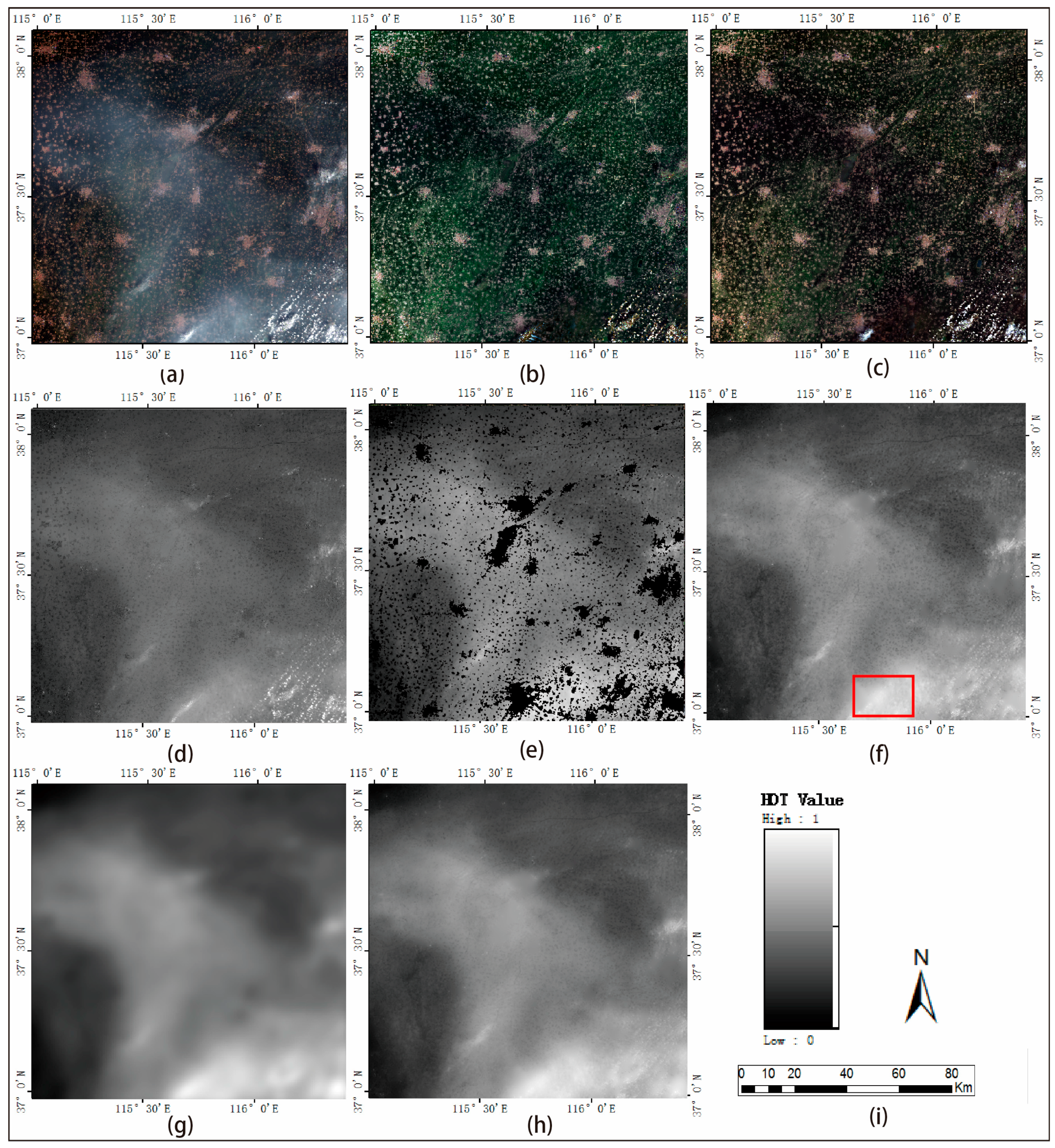
Finally, HOT transformation is applied to each pixel to generate a HOT map (hereafter H0) of the whole image through Equation (1). Figure 1d shows the HOT map of Figure 1a. Overall, HOT map reflects the relative intensity of the haze properly. However, spurious HOT responses also exist, especially in the regions corresponding to sensitive targets. If using it as the reference for DOS, serious color distortion would appear in the dehazed image, as shown in Figure 1b. Hence, refinement is required to gain a more accurate estimation. Figure 1e–h show all HOT maps during the process of HOT perfection and Figure 1c is the final dehazed result of our proposed method. Next, we give a detailed description of HOT perfection and percentile DOS.

2.2. HOT Perfection

2.2.1. Valid Pixel Set

Experiment in [10,12] proved that HOT combined DOS technique provided good results for vegetated areas. Thus, we can treat vegetation cover areas as effective region for utilizing HOT to assess relative haze thickness and the corresponding part in initial HOT map as valid pixel set. In order to extract the valid pixel set, we demand for a universal mask. The normalized difference vegetation index (NDVI) can achieve this goal easily since it owns the ability to assess whether the target being observed contains live green vegetation or not. The formula for NDVI is:

$$\text{NDVI}=({\rho }_{nir}-{\rho }_r)/({\rho }_{nir}+{\rho }_r)$$

(5)

where ${\rho }_{\mathit{nir}}$ and ${\rho }_r$ stand for the spectral reflectance measurements acquired in band near-infrared and red, respectively. The NDVI varies between −1.0 and +1.0. In general, the NDVI of an area containing a dense vegetation canopy will tend to positive values while clouds, water and snow fields will be characterized by negative values. In addition, bare soils tend to generate rather low positive or even slightly negative NDVI values. Hence, the threshold (hereafter T₁) between 0.1 and 0.3 of NDVI is suggested to extract dense vegetation.

However, in our experiments we find some man-made features whose colors are close blue or red are neglected. Observed that the absolute differences of these features between band blue and red are much higher than valid pixel set, we therefore recommend utilizing red-blue spectral difference (RBSD), equal to DNs of band blue minus that of band red, as an assistant. Their locations and boundaries are obvious in the grey-scale map of RBSD, thus the threshold (T₂) can be determined through histogram after two or three attempts of threshold classification. Combing NDVI with RBSD, a general mask can be designed to get rid of sensitive targets.

Pixels with NDVI values higher than T₁ and RBSD values lower than T₂ are regarded as valid pixels. Then, invalid pixels are masked out from H0 and the values of them are inferred from the valid pixel set. Figure 1e shows the masked-out HOT map.

2.2.2. Scanning and Interpolation

We adopt a four-direction scan and dynamic interpolation method to gain the filled value of masked-out areas, which can maintain the spatial continuity and local correlation of surface features. In this section, the detail of this method is described.

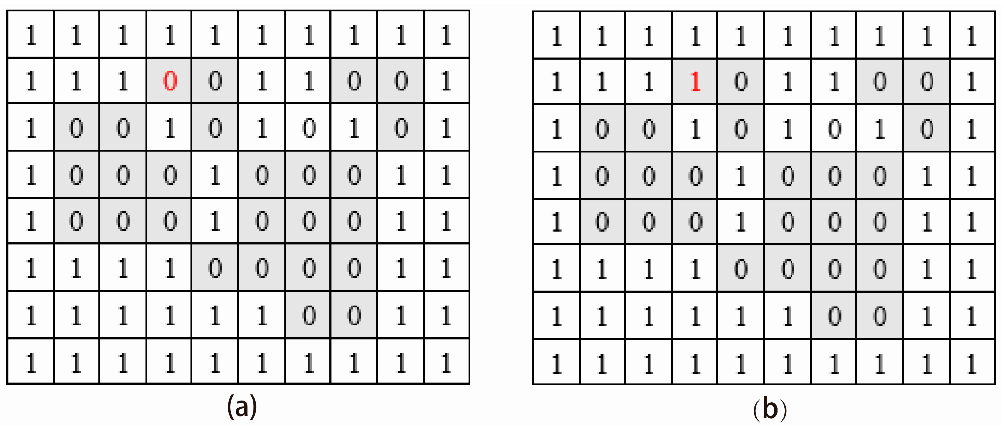
Assuming the valid pixels are labeled as 1 and others 0, we firstly consider a simple situation as shown in Figure 2a, whose masked-out areas are located inside the whole image. Next, start the first scan from the upper left corner following the direction from left to right and then top to bottom. When scanning to a pixel labeled 0 such as the pixel at row 2 and column 4, a local window with a radius of 3 pixels is used to search valid pixels surrounding it. The average HOT value of all valid pixels in this window is regarded as the value of that pixel and the value is filled into the current matrix. Now, the state of the matrix is as Figure 2b. The same process is repeated until reaching to the lower right corner. As the state of matrix is changed every time coming across a pixel labeled 0, this process is called dynamic interpolation.

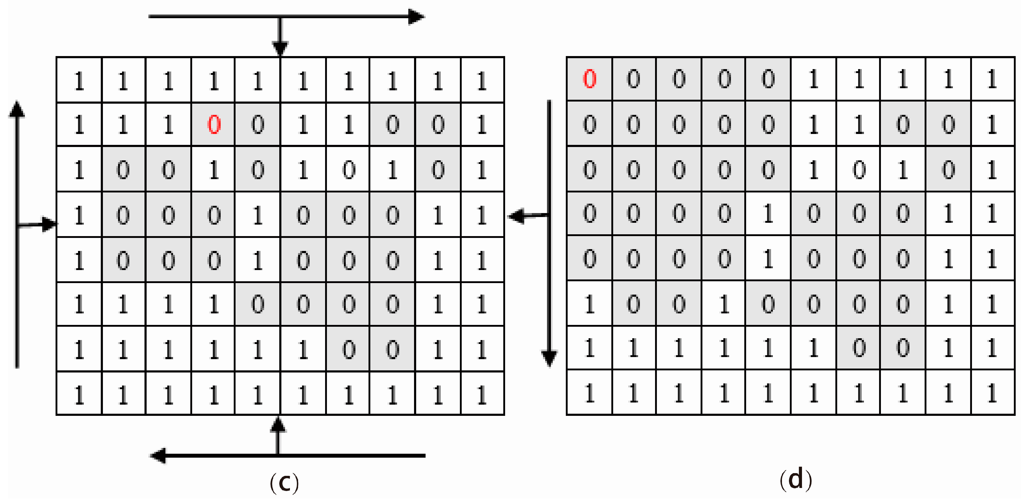
Then, scan the mask-out HOT map from the other three directions as shown in Figure 2c in which the long arrows represent the direction of scanning line and the short arrows stand for the moving direction of scanning line. It is stressed that four scans are independent of each other, originating from the initial masked-out HOT map. The four matrices of four scanning results are added up to compute the average to generate our final result of interpolation (hereafter H1).

More complex situation should be taken into consideration, such as Figure 2d. When scanning from the upper left corner and locating at row 1 and column 1, we cannot find any valid pixel in the pixel’s 3 × 3 neighborhood. Hence, its tag remains unchanged and its HOT value is still null. If we changed the starting point, such as upper right, this problem will be solved successfully. We find that all masked-out areas are surrounded by valid pixels in at least two directions of the four in Figure 2c. Thus, after four-direction scan and dynamic interpolation, all masked-out areas are filled and the influence of valid pixels in different directions has been delivered to the point to be interpolated. In addition, this process is efficient and only takes 13 s for an image of size 7771 × 7901 pixels.

Figure 1f shows the interpolation result of Figure 1e. Spurious HOT responses are corrected after interpolation and the contrast of different haze intensity becomes more vivid. However, another problem occurs in large-scale mask-out areas, such as water surface or thick haze. With the increase of distance, the influence of valid pixels is weakened, resulting in the lower HOT value of central pixels of a large masked-out regions than marginal pixels, such as the area labeled by red rectangular in Figure 1f. Therefore, compensating for these areas is required.

2.2.3. Homomorphic Filter for Compensating

There is a common characteristic of large-scale haze and water surface that their spatial distributions are locally aggregated and continuous. The property is transferred to the original HOT map through HOT transformation. Therefore, large-scale haze or clouds and water surface are assumed to locate in the low-frequency of H0 [22,23]. In this section, we utilize a homomorphic filter method to extract the low-frequency information of H0. The algorithm is described as follows:

(1)

H0 is expressed as Equation (6) [18]:

$$\mathbf{H}\mathbf{0}=f(x,y)=i(x,y)\times r(x,y)$$

(6)

where i(x,y) is the low-frequency information to enhance and r(x,y) is the noise to suppress.

(2)

Logarithmic transformation: convert the multiplicative process of Equation (6) to an additive one

$$z(x,y)=\text{ln }f(x,y)=\text{ln }i(x,y)+\text{ln }r(x,y)$$

(7)

(3)

Fourier transformation: transform z(x,y) from space domain to frequency domain F{z(x,y)} = F{ln i(x,y)} + F{ln r(x,y)}, simplified as:

$$Z(u,v)=F_i(u,v)+F_r(u,v)$$

(8)

where F_i(u,v) and F_r(u,v) represent the Fourier transformation of ln i(x,y) and ln r(x,y).

(4)

Filtering: use a Gaussian low-pass filter H(u,v) to enhance the low-frequency information including large-scale haze or water surface, and meanwhile suppress the high-frequency information including noise:

$$S(u,v)=H(u,v)Z(u,v)=H(u,v)F_i(u,v)+H(u,v)F_r(u,v)$$

(9)

and H(u,v) is defined as:

$$H(u,v)=\text{exp}[-\frac{D^2(u,v)}{2{{\sigma }_0}^2}]$$

(10)

${\sigma }_0$ denotes the cut-off frequency, u and v are the coordinates, and D(u,v) denotes the distance between the (u,v) coordinate and the origin of Z(u,v). The cut-off frequency, which is used to separate the high and the low frequencies, should be adjusted according to actual situation. In general, the smaller cut-off frequency means more enhancement of low-frequency information. In our experiments, ${\sigma }_0$ is fixed to 10.

(1)

Inverse Fourier transformation:

$$s(x,y)=F^{-1}\{s(u,v)\}$$

(11)

(2)

Exponential transformation:

$$g(x,y)=\text{exp}[s(x,y)]$$

(12)

Figure 1g shows the result of g(x,y) (hereafter H2) for Figure 1d. It can be seen that background noise relating to land cover types has been suppressed while the main or relative large-scale haze has been enhanced. H2 can be used to evaluate relative haze thickness at a large scale but may neglect some details, such as small haze patches or silk ribbons. H1 preserves the details but underestimate the haze thickness of large-scale haze or water surface. Thus, fusion of H1 and H2 can provide a more accurate estimation of haze. The final HOT map (hereafter H) is obtained as:

$$\mathbf{H}=\lambda \mathbf{H}\mathbf{1}+(1-\lambda )\mathbf{H}\mathbf{2}$$

(13)

where $\lambda \in [0,1]$ is used to weight the contribution of H1 and H2 in the final result. λ is fixed to 0.5 in our experiments unless otherwise stated. Figure 1h shows the final HOT map of Figure 1a.

2.3. Percentile DOS

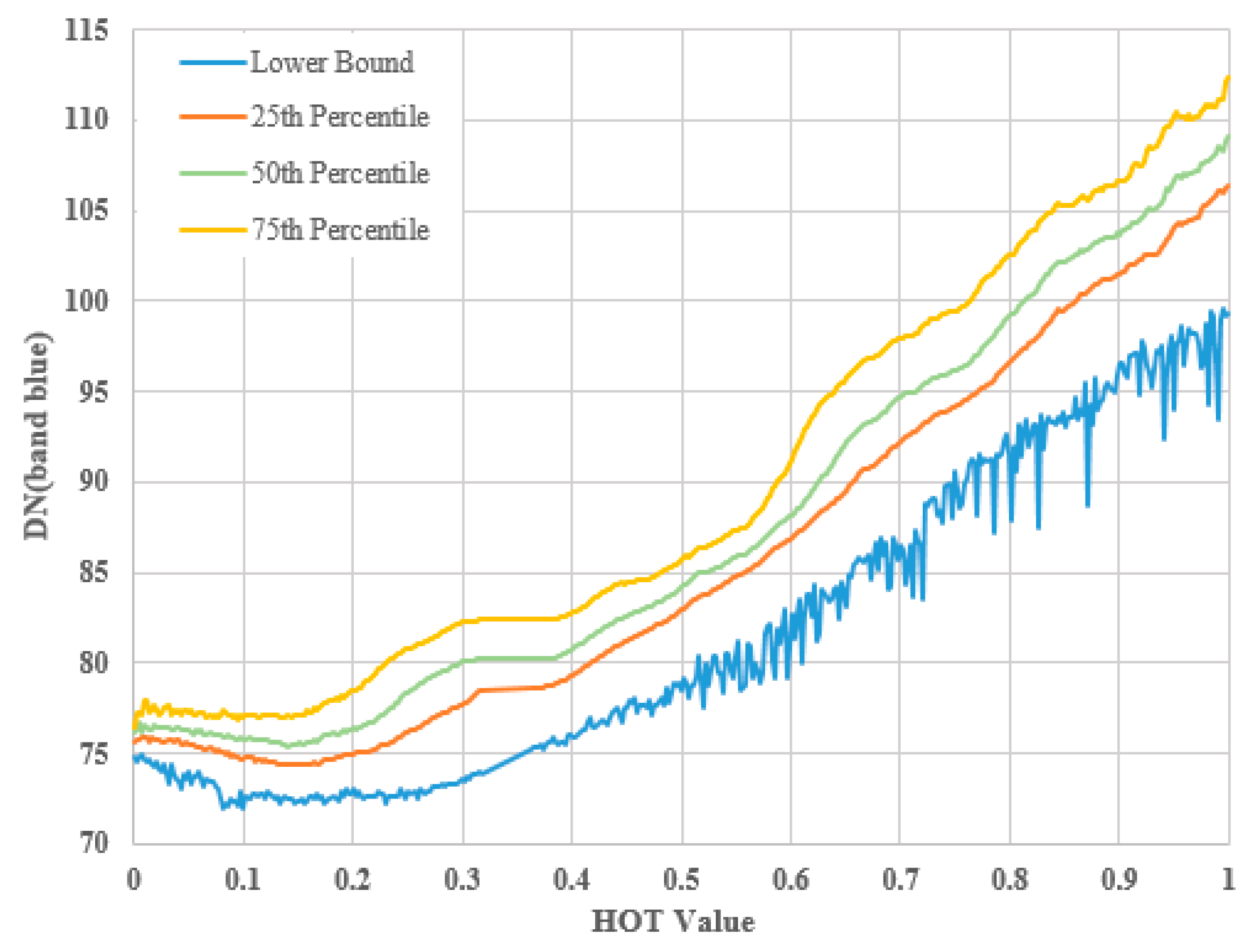
After HOT perfection, spurious HOT responses of sensitive targets have been eliminated and H provides us correct evaluation of relative haze thickness. If slicing each band of original images into different layers to ensure the HOT responses of each layer are the same or vary in a small range, we can consider the atmosphere condition of each layer is homogeneous and it becomes reasonable to apply DOS method for haze removal. Utilizing histograms of each layer, we determine a curve $\psi =\text{DN }(\text{HOT})$ (The blue curves in Figure 3 shows an example of band blue), reflecting the relationship between the lower-bound DN value and HOT level. We quantify the level of migration of a given layer by the offset of its lower-bound level relative to that of a selected reference layer and this migration determines the adjusted DN of pixels in this layer. For example, supposing the lower bound of the selected reference is 70 and that of a given layer ($\text{HOT}\in (0.50,0.55]$) is 87, the adjusted DN of pixels in this layer should be 17, equal to 87 minus 70. That is to say, pixels with an observed HOT level between 0.50 and 0.55 should have its DN of band blue reduced by 17 during the radiometric adjustment phase. In addition, we usually choose the minimal lower-bound value as the reference. This procedure is used to adjust all visible bands for which the histogram analysis has been done.

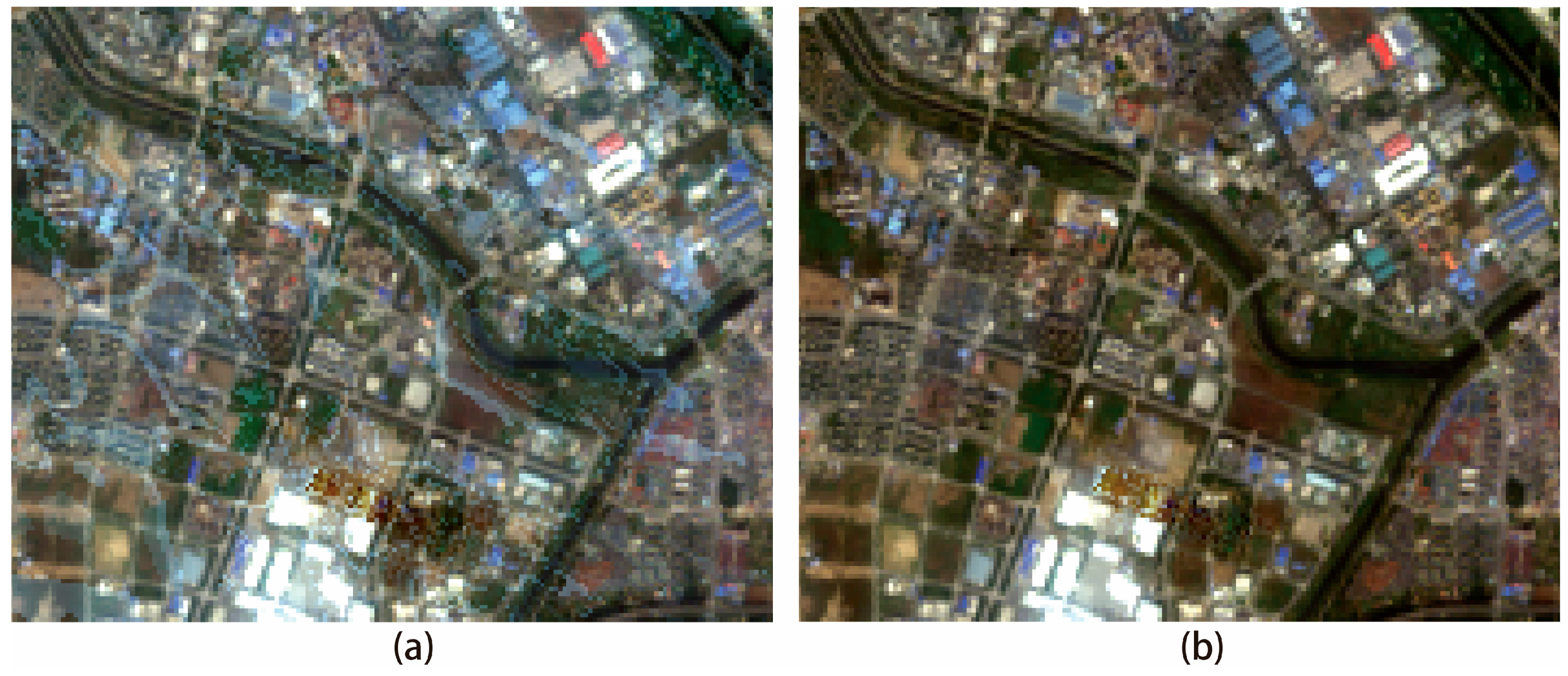
However, experiments show that the lower-bound values often appear unstable, especially for band blue which is notoriously noisier than others. Thus, the adjusted values determined by $\psi$ tend to jump up and down between adjacent HOT levels, finally leading to many patches and halo artifacts in the dehazed image, such as Figure 4a. An effective approach to solve this problem is to replace the lower-bound with percentiles of histograms. Figure 3 shows the curves of 25th/50th/75th percentiles for band blue, illustrating percentiles are more stable than the lower-bound. Hence, the adjusted values determined by percentiles between adjacent HOT levels will change smoothly. As a result, the dehazed image shows a stronger integrity and patches and halo artifacts disappear as shown in Figure 4b.

Haze removal above is a “relative” method as the effect of the atmosphere is just adjusted to a homogenous background level. The traditional DOS method is applied to finish our radiometric adjustment. Figure 1c shows the final haze removal result of Figure 1a.

3. Results

To test the effectiveness of our proposed methodology, we applied it to several scenes covering representative surface cover types including sensitive targets and encompassing a broad spectrum of atmospheric conditions. The data used in our study includes Landsat 8 OLI and GF-2 images. Spatial resolution of the former is 30 m and that of the latter is 4m in visible and near-infrared spectral bands. The thresholds of NDVI in our experiments are determined according to the criteria in Section 2.2.1 unless otherwise stated.

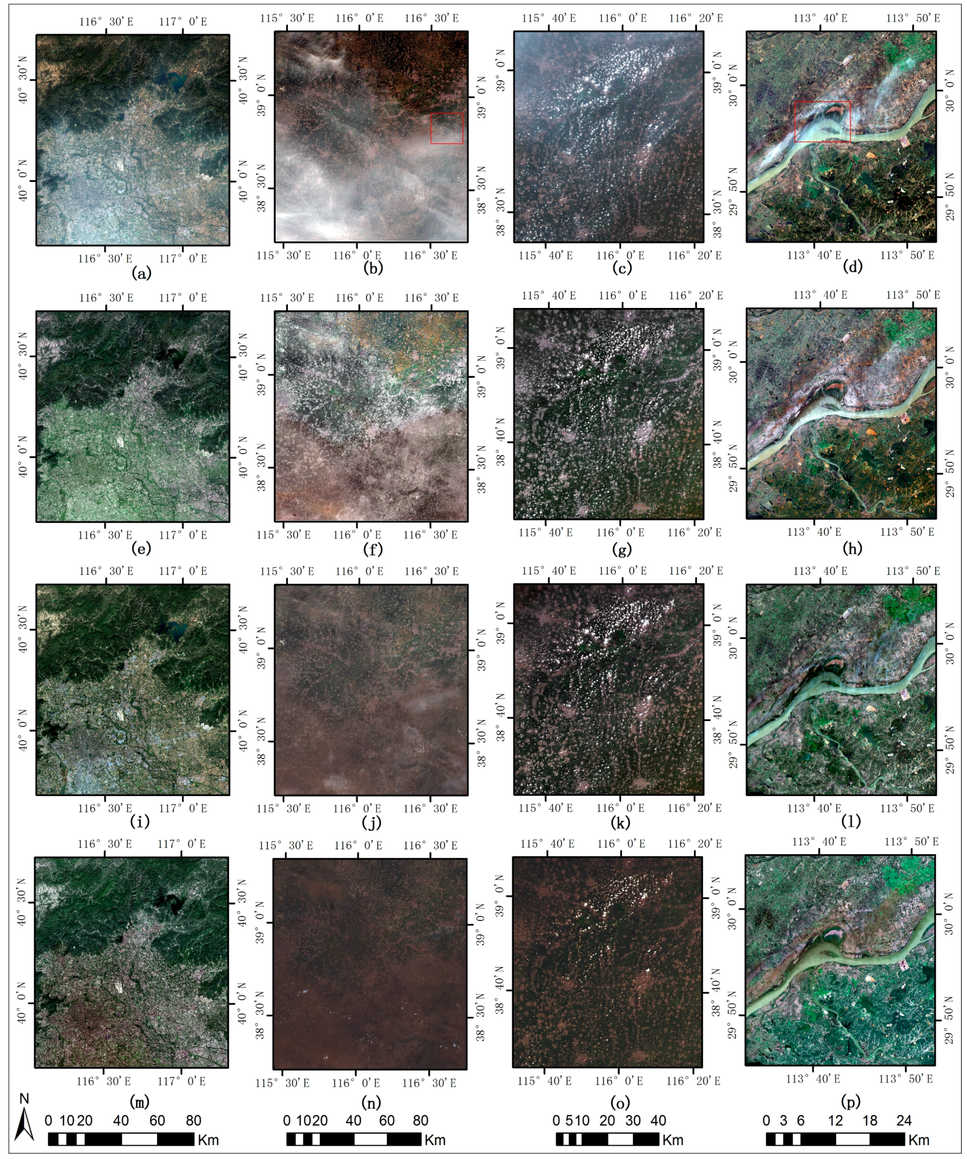
Figure 5 shows the result of haze removal of Landsat 8 OLI data, whose parameters are listed in

Table 1. Parameters of the Landsat 8 OLI data sets.

	Figure 5a	Figure 5b	Figure 5c	Figure 5d
Landsat scene ID	LC81230322013276LGN00	LC81230332015266LGN00	LC81230332015218LGN00	LC81230392016157LGN00
WRS path	123	123	123	123
WRS row	32	33	33	39
Acquired date	3 October 2013	23 September 2015	6 August 2015	5 June 2016
Solar elevation angle	43.30°	47.67°	60.83°	69.06°
Solar azimuth angle	156.79°	152.03°	133.12°	106.44°

. The results of the proposed method are compared with those of original HOT and BSHTI. Visually, all of the three methods can remove haze and thin clouds to a certain degree by correcting the values of the hazy pixels. However, the color cast is serious in the results of original HOT, and the spectra of the clear pixels are changed as well as the cloudy pixels, as the second row of Figure 5 shows. Contrarily, the result of the proposed method is pleased with a good apparent recovery of surface detail and it preserves features’ natural color properly, as shown in the third row of Figure 5. Overall, the proposed method removes haze and thin clouds while fragmentary small haze patches or silk ribbons remain, which correspond to thick cloud in original images, especially in Figure 5j. BSHTI removes haze and clouds completely, as the last row of Figure 5 shows. 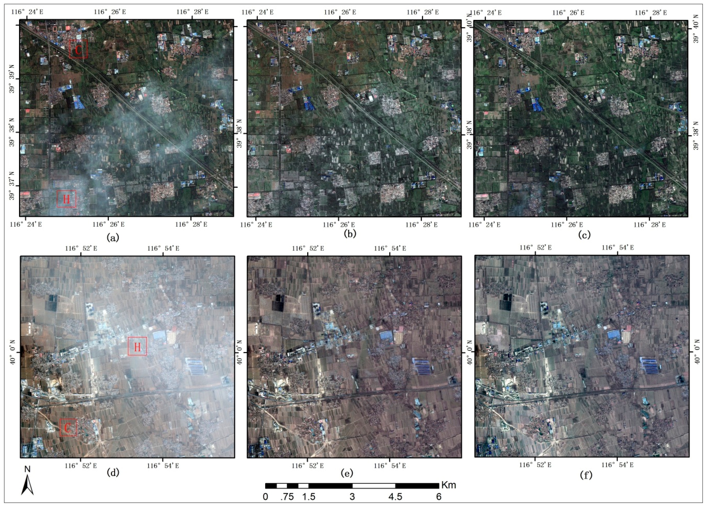However, there exist unexpected patches and halo artifacts in dehazed results which appear at the junction between thin and thick haze regions, especially in the lower-right corner of Figure 5n. Furthermore, we select two typical samples for careful comparison of the proposed method and BSHTI in Figure 6. Their locations are labeled in Figure 5 by red rectangle.

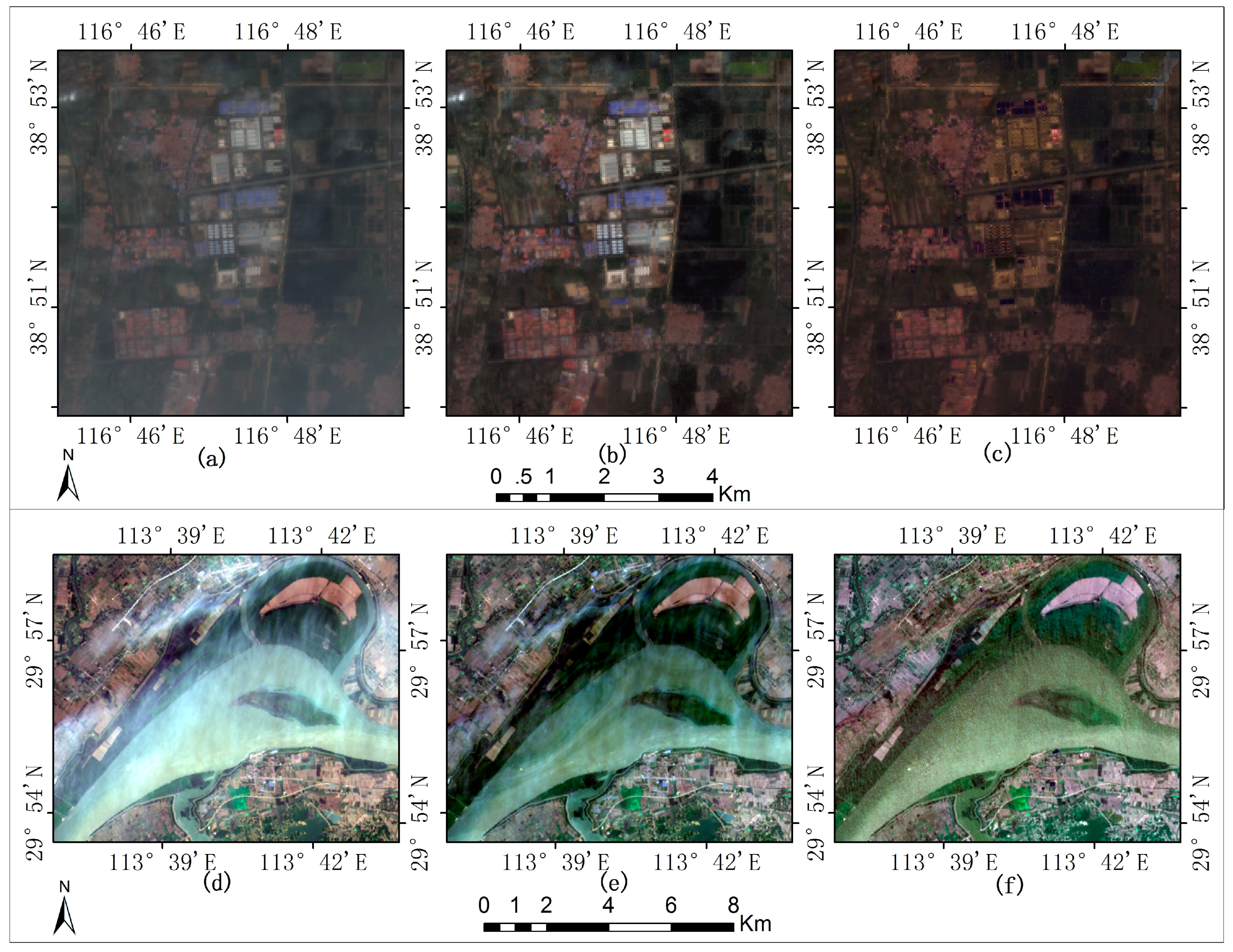
Figure 6a covers a suburban area including many colorful man-made features. The proposed method wipes out haze entirely and visibility of dehazed image has been significantly improved. Houses are clearly visible and the boundaries of them can be easily distinguished. By contrast, it becomes more difficult to distinguish houses in Figure 6c since their boundaries are mixed up with surrounding land cover types. Meanwhile, the colors of man-made features is changed greatly. This indicates that the proposed method behaves well in enhancing local contrast and preserving features’ natural color compared with BSHTI. A possible reason may be that BSHTI has treated all cover types as background noise without distinction, resulting in weakness of the differences between different types in its results. Similar situation occurs in Figure 6f, in which boundaries of riversides are blurred. The color of the transition zone from the river to land is very close to that of water surface, contrary to the reality. In fact, BSHTI has changed the color and texture of water surface compared to the original image while the proposed method maintains the general tone of the original image, as shown in Figure 6e. In addition, it seems that the small island in the river becomes a little smaller along with the erosion of its boundary, which implies that BSHTI might have destroyed the structure of the original image in the process of removing haze.

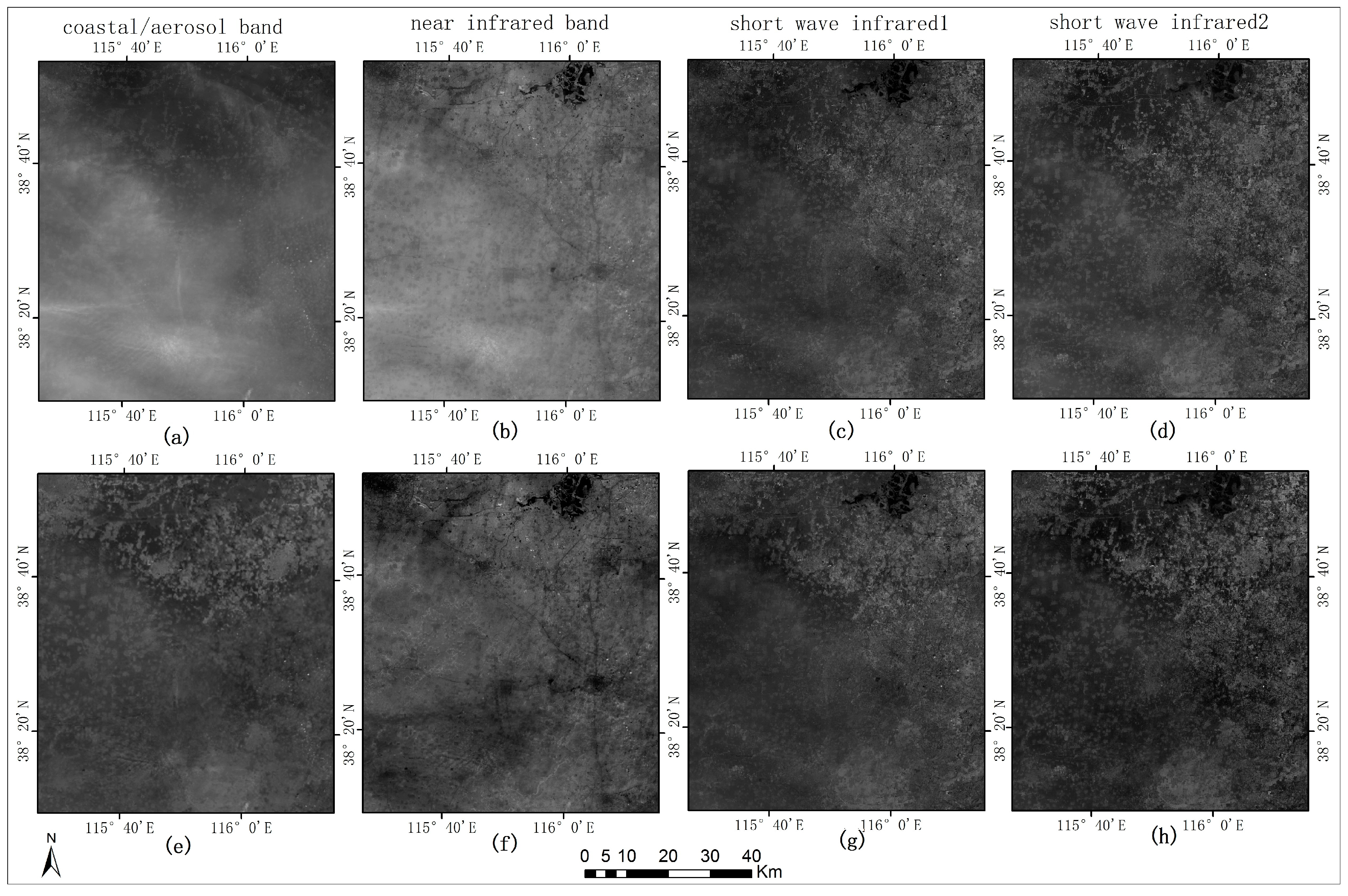
Although our proposed method is initially designed to remove haze in RGB channels, we find that the method is also suitable for haze removal in other bands, such as coastal/aerosol band (band 1), near infrared band (band 5), and short wave infrared (band 6, and band 7) of Landsat 8 OLI data. In general, longer wavelengths of the spectrum are influenced by haze much less. Thus, we just cut out the subset of Figure 5b which is affected relative seriously in longer wavelength for an observation of dehazed effect on these bands. Figure 7 shows the dehazed results in other spectral bands of Landsat 8 OLI data. It is clear that the effect of haze has been eliminated and visibility of results has been significantly enhanced.

Figure 8 shows the results of haze removal on GF-2 images with a spatial resolution of 0.8 m after fusing full-color and multi-spectral bands. The image of Figure 8a is acquired on 2 September 2015 containing rich green vegetation. The image of Figure 8d covers a rural area locating at the northern of China and it is acquired on 12 February 2015 when crops have not grown up. The lack of dense vegetation makes it difficult to implement the proposed method since the valid pixels are not enough to infer out HOT values of masked-out regions. Thus, the previous criteria (varying in 0.1–0.3) for the determination of the NDVI thresholds becomes unsuitable in this case. We have achieved the goal of removing haze by means of lowering the threshold of NDVI (varying between −0.2 and −0.1) when designing the general mask. Overall, both methods provide us with intuitively content dehazed results. That is to say, our proposed method and BSHTI are also suitable for eliminating haze of high-resolution satellite images.

For Figure 8, the color of bare soil in our results is more in line with the real state than that of BSHTI’s. In the upper left corner of Figure 8b, the boundary of bare ground and the surrounding vegetation is clear, and the color difference is obvious, whereas small bare soil blocks are mixed up with vegetation around them and their areas turn to become small in Figure 8c. As for Figure 8f, the color of the whole image seems close green, which may lead to the wrong judgment that there is a lot of green vegetation on the surface.

According to the experimental results, we can come to the conclusion that the proposed method provides a more satisfying result for haze removal. All mentioned above suggest that the proposed method is more capable of preserving the natural color of object itself, enhancing local contrast, and maintaining the structural information of original images. However, our analysis is likely to be biased as it can be influenced by different perspective or personal preference. Thus, more objective discussion should be introduced to determine which method is a high-quality implementation of haze removal. In the next section, three indices are chosen for our discussion.

4. Discussion

4.1. Quality Assessment of Dehazed Results

It is known that haze removal is a pre-processing step for subsequent applications or information extraction. Thus, our haze removal methods should provide us with results which are helpful for computer recognition and classification under the premise of ensuring accuracy. We consider less image distortion, higher structural similarity and stronger local contrast as the basic criterion to be met. Therefore, we choose three quality assessment indicators to evaluate our results: (1) Visual Image Fidelity (VIF) [24] to measure difference of pixels before and after haze removal; (2) Universal Quality Index (UQI) [25] to compare the structural similarity of images; and (3) Contrast-To-Noise Ratio (CNR) [26] to evaluate local contrast enhancement of dehazed results. We briefly review them in the following.

VIF relies on three models: Natural Scene Statistics model, distortion (channel) model and Human Visual System (HVS) model. VIF models natural images in the wavelet domain using Gaussian Scale Mixtures and assumes the coefficients in the wavelet domain are uncorrelated. It explains visual distortion of human vision as the noise of internal neurons. VIF is defined as Equation (14):

$$VIF={\displaystyle \sum _{j=1}^K[I({\stackrel{\rightharpoonup }{C}}^{N,j};{\overrightarrow{F}}^{N,j}|s^{N,j})]}/{\displaystyle \sum _{j=1}^K[I({\stackrel{\rightharpoonup }{C}}^{N,j};{\stackrel{\rightharpoonup }{E}}^{N,j}|s^{N,j})]}$$

(14)

where C and s denotes the vector and scalar random field from the reference signal; and E and F denote visual signal at the output of HVS model from the reference and the test images, respectively. $I({\stackrel{\rightharpoonup }{C}}^N;{\stackrel{\rightharpoonup }{E}}^N|s^N)$ and $I({\stackrel{\rightharpoonup }{C}}^N;{\overrightarrow{F}}^N|s^N)$ represent the information that could ideally be extracted by the brain from each-band in the reference and the test images, respectively. K represents the total numbers of sub-bands.

UQI is a mathematically defined image quality assessment index. Let $\mathbf{x}=\left\{x_i\right|i=1,2,\dots ,N\}$ and $\mathbf{y}=\left\{y_i\right|i=1,2,\dots ,N\}$ be the reference and the test image signals, respectively. The mathematical definition of UQI is given by Equation (15):

$$UQI=\frac{4{\sigma }_{xy}\overline{x}\overline{y}}{({{\sigma }_x}^2+{{\sigma }_y}^2)[{(\overline{x})}^2+{(\overline{y})}^2]}$$

(15)

where $\overline{x}=\frac{1}{N}{\displaystyle \sum _{\mathrm{i}=1}^{\mathrm{N}}{x}_i}$, $\overline{y}=\frac{1}{N}{\displaystyle \sum _{\mathrm{i}=1}^{\mathrm{N}}{y}_i}$, ${{\sigma }_x}^2=\frac{1}{N-1}{\displaystyle \sum _{\mathrm{i}=1}^{\mathrm{N}}{(x_i-\overline{x})}^2}$, ${{\sigma }_y}^2=\frac{1}{N-1}{\displaystyle \sum _{\mathrm{i}=1}^{\mathrm{N}}{(y_i-\overline{y})}^2}$, and ${\sigma }_{xy}=\frac{1}{N-1}{\displaystyle \sum _{\mathrm{i}=1}^{\mathrm{N}}(x_i-\overline{x})(y_i-\overline{y})}$.

CNR is similar to signal-to-noise ratio (SNR), but is based on a contrast rather than the raw signal. CNR provides us with more precise evaluation than SNR when there is a significant bias in an image resulting from haze et al. One way to define contrast-to-noise ratio is:

$$CNR=\frac{\left|S_A-S_B\right|}{{\sigma }_N}$$

(16)

where S_A and S_B are signal intensities for signal structures A and B, respectively; and ${\sigma }_N$ is the standard deviation of the image noise. In [20], two Gaussian kernels are used to estimate structure B and image noise while the original input image are used as structure A. It is stated that the value of CNR in

Table 2. Image quality assessment results for dehazed images.

	VIF		UQI		CNR
	PM *	BSHTI	PM	BSHTI	PM	BSHTI
Figure 5b	−0.0766	−0.1105	0.8481	0.6868	4.2339	−7.8331
Figure 5c	−0.0015	−0.0041	0.8367	0.6320	4.7505	−0.7602
Figure 8a	−0.0297	−0.0594	0.8038	0.6455	4.7502	−4.5422
Figure 8d	−0.0452	−0.0276	0.4698	0.3989	−4.8098	−11.4610

* PM means the proposed method.

is not the direct computing result according to Equation (16). In order to expose the change before and after haze removal, we use the differences of CNR values between the original images and dehazed results as the values listed in Table 2.

Table 2 lists the values of different objective quality assessment indices for haze removal results of Figure 5b,c and Figure 7a,d, which are subsets of the whole images. The original hazy data are used as the reference images and dehazed results are the test images. It is stressed that all these values are calculated in RGB channels.

In general, the closer VIF gets to zero, the less serious image distortion. According to the data, some distortions happen in all dehazed images. However, this does not mean the true distortion in dehazed results because there could be great differences between the pixels in original image and haze removed image especially when heavy haze exists. Thus, the image distortion in our results is acceptable and it can come down to the direct consequence of haze removal. For Figure 5b,c and Figure 7a, VIF values of the proposed method are much closer to 0 than BSHTI while it is inverse for Figure 8d. Regarding these statistical values, it implies that the proposed method behaves well in most cases while BSHTI is more capable of dealing with the situation where there is a lack of vegetation. For Figure 5b, the absolute values of VIF are much larger than others, which is in accord with the fact that Figure 5b contains much heavier haze.

The structural similarity is independent of the contrast and color of the image. It can be seen that both methods gain relatively high values of UQI, which means strong ability to preserve structural information. The contrast of UQI indicates that the proposed method is superior to BSHTI in this aspect. Meanwhile, note that UQI values of Figure 5b,c and Figure 7a are much larger than those of Figure 8d, which implies that we can benefit from dense vegetation when removing haze and CNR shares the same characteristic.

For the first three figures, CNR values of the proposed method are positive values while that of BSHTI are negative numbers, that is to say, the local contrast has been enhanced in the haze removed image of the proposed method while weakened in the result of BSHTI. Whereas, the proposed method also shows poor effect on local contrast enhancement for Figure 8d. It proves again that the proposed method would benefit from dense vegetation in some way. Nevertheless, we can consider the proposed method as an outstanding one to clear out the influence of haze since all results of it have larger CNR values compared with BSHTI’s.

In summary, the discussion above leads to the conclusion that the proposed method is superior in maintaining structural information of original image and enhancing local contrast to BSHTI based approach. Both methods lead to image distortion in haze removal results more or less but it is acceptable.

4.2. Analysis of Spectral Consistency

A quantitative evaluation of a dehazing method is a difficult task as the appropriate hazy data together with ground truth are difficult to collect. Since a strict validation is not possible, we choose a pair of hazy and haze-free images for analysis of spectral consistency. The images have minimal time difference and minimal difference of the Sun/sensor geometry, which allows us to use the haze-free image as a reference and to perform an evaluation of the dehazing method by a comparison of the spectral information. The detailed information on the data is given in

Table 3. Parameters of hazy and haze-free (reference) data sets.

	Hazy	Haze-Free (Reference)
Landsat scene ID	LC81960292013195LGN00	LC81970292013186LGN00
WRS path	196	197
WRS row	29	29
Acquired date and time(UTC)	14 July 2013, 10:25:28	5 July 2013, 10:31:39
Solar elevation angle	61.99°	63.11°
Solar azimuth angle	138.04°	137.32°

.

Figure 9 illustrates the dehazed results for a Landsat 8 OLI sub-scene. Visual interpretation of the dehazed image (Figure 9b) and comparison to the reference (Figure 9c) using a true color RGB composition confirm that the proposed method performs well. We intend to compare the channel intensity profiles in the hazy, dehazed and reference image to analyze the spectral consistency. Figure 10 presents band profiles (Figure 9a, vertical red line) of coastal/aerosol band (band 1, 0.433 μm), blue band (band 2, 0.483 μm), near infrared band (band 5, 0.865 μm), short wave infrared1 (band 6, 1.610 μm) for the original hazy (red line), dehazed (green line) and reference (blue line) images.

The original and dehazed profiles have similar shapes in the haze-free region (right part of the graph in Figure 10), illustrating that the dehazing process outside the haze regions does not modify the spectral properties of the original data. Meanwhile, these two spectra have the same shape as the reference image spectrum. In the hazy region (left part of the graph), the dehazed profile illustrates a noticeable dehazing enhancement of the band intensities together with a preservation of the surface structure as it has the same shape as the profile of the reference image. It means that the method produces spectrally consistent dehazed data. The difference between the dehazed and reference spectra can be attributed to residual scene coregistration errors, different atmospheric conditions, and residual haze thickness errors. The differences in long wavelength range are minimal due to the weak effect of haze and atmospheric conditions.

We have applied the proposed method to a full-size Landsat 8 OLI data (3 October 2013; scene ID: LC81230322013276LGN00), whose size is 7771 × 7901 pixels. The result is partially displayed in Figure 5i. The execution time to handling four bands (RGB and NIR) is approximately 506 s on Intel Xeon E3-1225, using an MATLAB implementation of the algorithm.

In all, the proposed method produces high-fidelity and spectrally consistent haze removal results. The color of RGB composites is close to that in reality, which is helpful for visual interpretation. Spectral consistency ensures that haze removal would not influence other algorithm relying on spectral information of images. The dehazed data are expected to be used as data sources of land cover classification and mapping, surface change detection and other applications involving ground information extraction.

5. Conclusions

In this paper, we propose a high-fidelity haze removal method for visible remote sensing data. This method is effective in removing haze and thin clouds and can result in haze-free images with high color fidelity. Three steps are included in our proposed method: semi-automatic HOT transform, HOT perfection and percentile DOS. First, a non-overlapping window is utilized to search the relative clearest regions of the whole scene automatically through the R-squared criterion. Second, NDVI and RBSD are used to design a general mask for the sake of masking out spurious HOT responses from the original HOT map. The masked-out areas are filled by means of four-direction scan and dynamic interpolation, and then homomorphic filter is performed to compensate for loss of HOT of masked-out regions with large areas. Then, each band of original images is sliced into different layers according to different HOT responses and percentiles of histograms are utilized to determine the adjusted DNs of each layer. Finally, DOS procedure is implemented to eliminate the influence of haze.

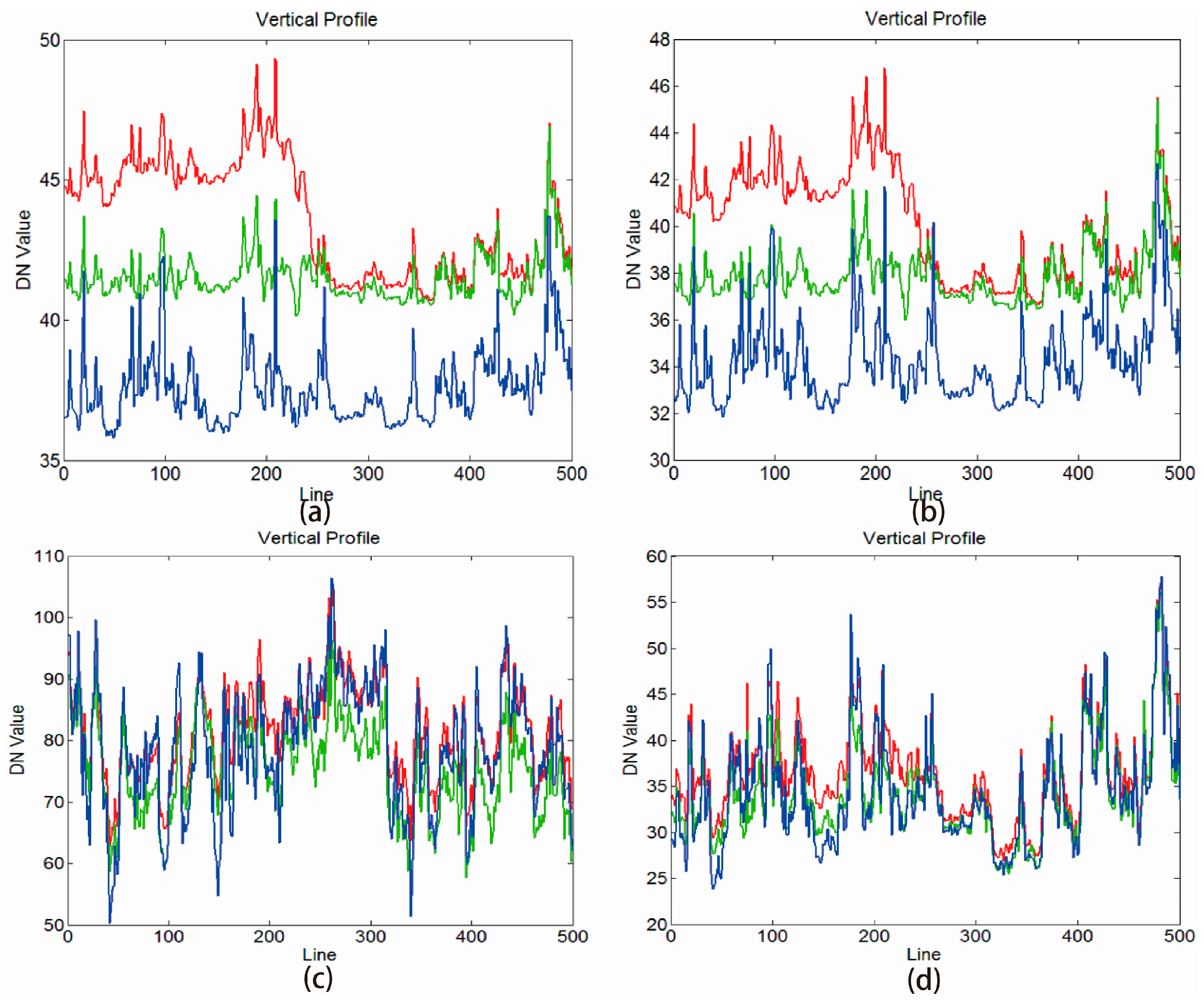
Experiments on several remote sensing data with medium and high spatial resolutions, including Landsat 8 OLI and GaoFen-2 images, validate the effectiveness of the proposed method. The halo artifacts are significantly smaller in our dehazed results. Image distortion exists in haze removal results more or less but it is acceptable. Comparative analysis verifies that the proposed method is superior in preserving the natural color of object itself, enhancing local contrast, and maintaining structural information of original images. As BSHTI treats all land cover types as background noise without distinction, differences between objects are weakened which leads to difficulty in land cover classification and mapping. Band profiles show that the dehazed result shares the similar spectral characteristic with the reference (haze-free) image in all spectral bands.

However, the proposed method is out of work at the area or in the season of sparse vegetation as it depends on a valid pixel set, such as the northwest arid area, the northern winter. Meanwhile, patches and halo artifacts arise in the results of Gaofen-2 images when zooming in the resulting image to a large scale. We consider it a substantial limitation of this method in view of that slicing the image might destroy the local integrity of land cover types. Anyway, it indicates the requirements of further improvements.