1. Introduction
Very high resolution (VHR) remote sensing images are images with very high spatial resolution. Higher spatial resolution remote sensing images not only exhibit better visual performance but also allow us to acquire a large amount of detailed ground information in urban areas. Thus, the potential applications of remote sensing, such as land cover mapping and monitoring [
1], human activity analysis [
2], and tree species classification [
3], have increased. Numerous practical applications based on VHR remote sensing depend on classification results. However, given the limitation of remote sensing technology, VHR images are often coupled with poor radiometry, with less than three or five spectral bands. Therefore, this characteristic (i.e., a high spatial resolution but poor spectral radiometry) does not necessarily reflect higher classification accuracies when the images are applied in practice [
4,
5,
6].
Spatial features based on pixel-wise analysis are usually employed to improve the performance of VHR image classification. Zhang et al. proposed the pixel shape index to describe the spatial information around the central pixel [
7]. Fauvel et al. presented a spatial-spectral classification method using SVMs and morphological profile (MP) [
8]. In addition, morphological profiles (MPs) with different structural elements were proposed for structural feature extraction and classification of VHR images [
9]. In previous studies [
4,
10], the spatial feature is combined not only with the spectral feature but is also often integrated with others. Many previous studies have demonstrated that high classification accuracies can be obtained by exploring the spatial features of VHR images in a pixel-wise manner. However, spatial–spectral feature-based methods depend on the performance of the spatial feature extraction algorithm and are usually data dependent. Any methods cannot be labeled as either a good or bad classification method [
5], because although the high spatial resolution provides the possibility of detecting and distinguishing various objects with an improved visual effect, the classification of VHR images usually suffers from uncertainty regarding the spectral information, because the increase of the intra-class variance and decrease of the inter-class variance lead to a decrease of the separability in the spectral domain, particularly for the spectrally similar classes. In other words, as different objects may present similar spectral values in a VHR image, it is a difficult task to extract reasonable spatial features in practical application.
Object-based techniques have been proposed for VHR image classification to solve the above problems, which are brought about by the higher resolution and lower spectral information of the VHR images [
11]. Object-based approaches usually start with segmentation to generate the image object, and an image object is formed by a group of pixels that are spectrally similar and spatially contiguous [
12,
13,
14]. Recently, object-based classification methods for VHR remote sensing images have been studied extensively in practical applications [
14,
15,
16,
17,
18]. For example, object-based spatial feature extraction has been proposed. This method aims to explore the relationship between each image object and its surrounding objects in the spectral and spatial domains. Zhong et al. defined an object-oriented conditional random field classification system for VHR remote sensing images, and the system utilized conditional random fields to extract contextual information in an objective manner [
19]. Zhang et al. proposed an object correlative index that can describe the shape of a target in an objective manner [
20]. Aside from the two aforementioned analyses, other powerful tools that maximize the spatial information of VHR image have been proposed for VHR images classification. These methods include graph theory [
21], semantic clustering algorithm [
22], and fuzzy rule-based approach [
23]. As the analysis scale increases from a single pixel to an object, more features (such as texture, shape, and length) can be obtained than when a single pixel is used, and salt-and-pepper noise has usually been alleviated in the classification map of a VHR remote sensing image. Comparisons between pixel-wise and object-oriented approaches were conducted. The object-based approach demonstrated certain advantages in terms of classification results [
24,
25,
26,
27]; for instance, that it can smooth the noise in the classified map and that more image features (e.g., the texture and shape of the object) can be utilized. However, several limitations of the object-based approach to VHR image classification relative to a pixel-based approach were found. For example, although some scale estimate approaches have been proposed [
28,
29,
30,
31], it is still difficult to determine the optimal segmental scale parameters [
32,
33].
Aside from pixel-wise and object-based VHR image classification methods, a multi-scale strategy is an effective approach toward improving the classifying performance of VHR images. Bruzzone et al. revealed a multi-level context-based system for VHR classification. The system aimed to obtain accurate and reliable maps both by preserving geometrical details in images and properly considering multilevel spatial context information [
34]. Huang et al. revealed a multi-scale feature fusion approach for the classification of VHR satellite imagery [
35,
36]. Johnson et al. proposed a competitive multi-scale object-based approach for land cover classification by using VHR remote sensing image [
37]. All the aforementioned works have verified that multi-scale feature extraction or multi-level system can effectively increase classification accuracy. Scale influence was also crucial in the classification of VHR images [
38]. However, lots of papers focused on spectral–spatial feature extraction algorithms, object-based, or multi-scale based approaches for VHR image classification. To our knowledge, few techniques specifically focus on the influence of the image scene scale on the classification of VHR images. Moreover, from s theoretical viewpoint, classification accuracy can be improved by increasing the number of representative training samples for a supervised classifier, and this can be found in the existing literature [
39,
40]. Therefore, on the contrary, it is interesting to investigate how to improve the classification accuracies through decomposing the complexity of the image content in the case of pre-defined training samples.
In this paper, we attempt to improve the classification accuracy through reducing the complexity of image content, and propose a generalized system based on observational scene scale decomposition (OSSD) to improve the performance of VHR image classification. Unlike other methods presented in the literature, the proposed OSSD-based system is general and data-independent.
The rest of the paper is organized as follows:
Section 2 presents a detailed description of the proposed OSSD-based system for classification of VHR imagery.
Section 3 presents the dataset used for experiments and reports the experimental results. Finally,
Section 4 provides a discussion of the proposed approach and concludes the paper.
2. The Proposed OSSD-Based Classification Method
In theory, the boundary among classes is more distinct, and a classifier can separate them more easily. However, because of the high spatial resolution and insufficient spectral information in a VHR image, intra-classes may have different spectral values, and the same spectral value may indicate different classes. Thus, determining the boundary between classes is difficult. Furthermore, spatial arrangement and spectral heterogeneity on the earth’s surface are complex. In general, a larger geographic area may contain more classes. By contrast, a smaller area may cover fewer classes. Considerably complex image content will make classification difficult. Thus, an interesting task is to investigate whether observational scale decomposition can allow a supervised classifier to achieve a better boundary and obtain a higher accuracy than without any observational scene scale decomposition.
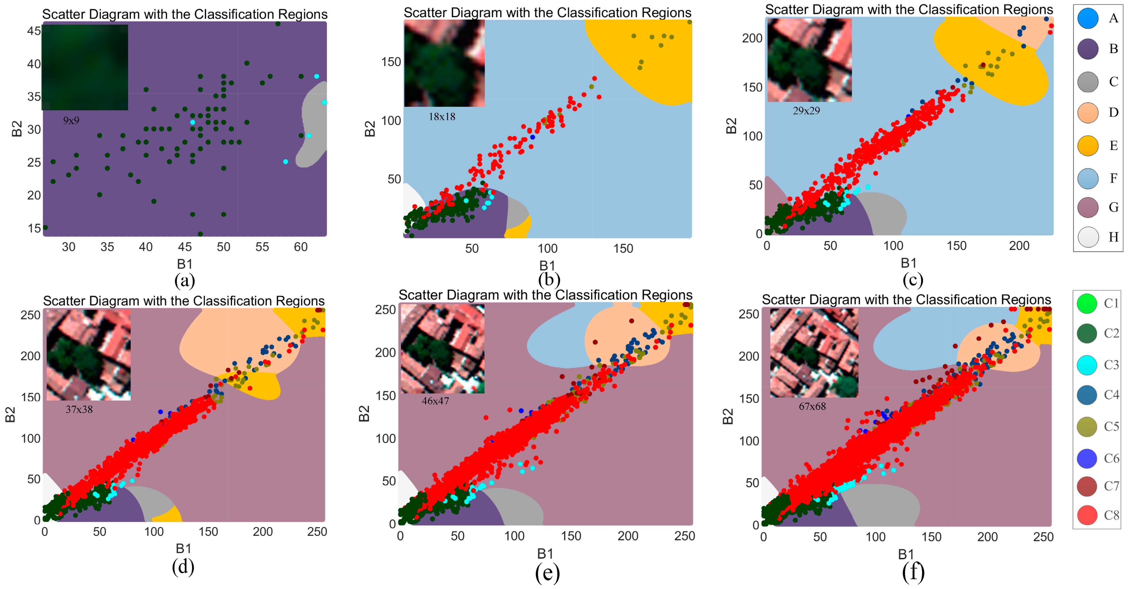
To verify our deduction, a primary example with different sized images is shown in
Figure 1, where the image block is extracted from an aerial image that is acquired by an ADS-80 sensor with three false-color bands and high spatial resolution. The image content becomes increasingly complex as the image size increases. In this comparison, bands 1 and 2 are the input features. Based on the pixels’ distribution in the feature space, the classification region is predicted by using a support vector machine (SVM) classifier with a Radial basis function (RBF) and a five-fold cross-validation. Data points are related to each pixel of the upper-left image. The training sample is set to ensure the fairness of each prediction. In
Figure 1, region “A” matches with class “C1,” region “B” matches with class “C2,” and so on. It can be found that the distribution of each class is greater mixed with the increase of the image size, meaning that more points are misclassified compared with the related region.
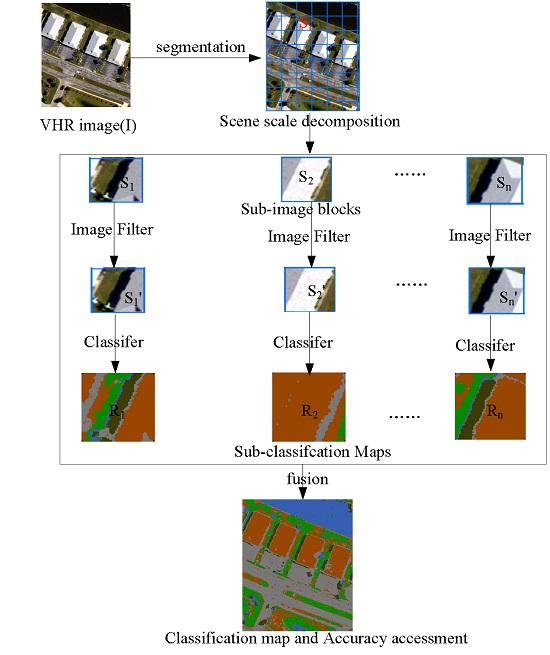
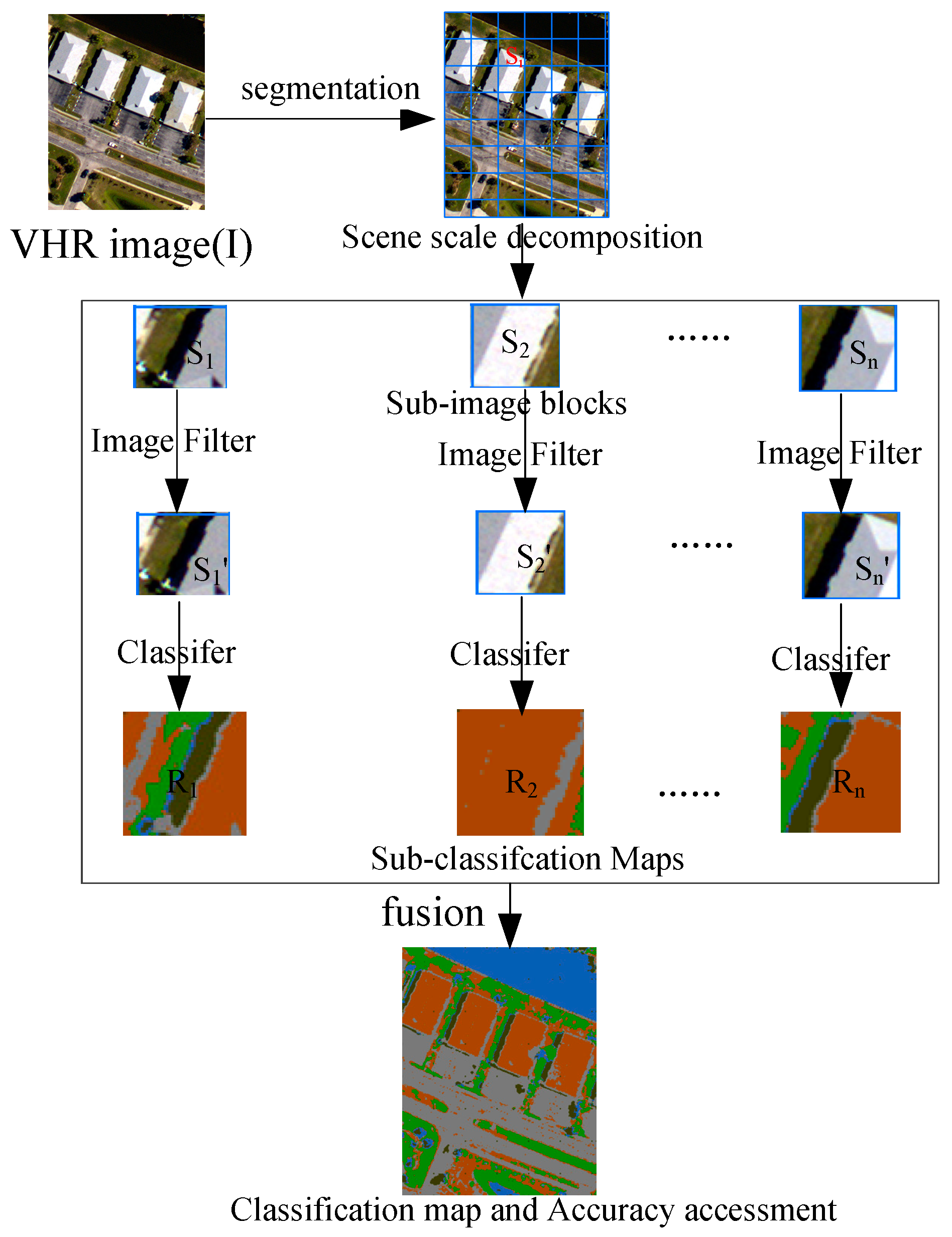
Therefore, exploring the relationship between image content decomposition and its classification accuracies is valuable and significant. To achieve this purpose, an image will be decomposed into sub-image blocks, each of which is classified. The flowchart of the proposed OSSD-based classification system is shown in
Figure 2. Three main blocks are contained. First, the whole image
is segmented by chessboard segmentation, and the image scene is decomposed according to the segmental vector. Second, each sub-image block (
) can be classified directly, or each sub-image block is processed through a filter, e.g., a median filter, to remove noise, and the filtered result is given as
Then, each band of the sub-image block is taken as the input feature for a classifier, and the classification result is
. Finally, the accuracy is evaluated based on the classification map, which is fused using each sub-image classification. In
Figure 2,
n is the number of sub-image blocks.
2.1. Scene Decomposition Using Chessboard Segmentation
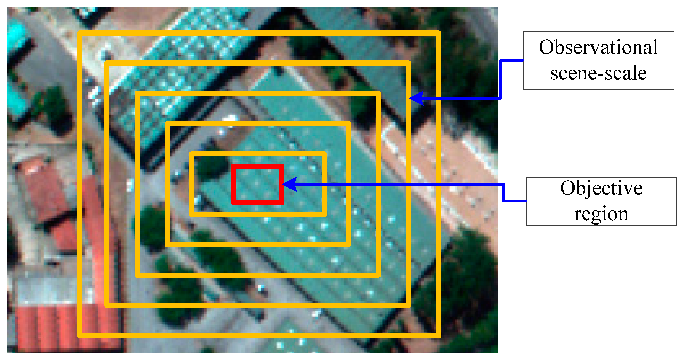
OSSD is adopted to limit spatial range and reduce the image complexity for classification. Observational scene scale is defined as the range of a sub-image block, as shown in
Figure 3. In theory, a smaller observation scene scale corresponds to lower complexity of a sub-image block, because more targets will be covered for classification as the observational scene scale increases. Therefore, the observational scene scale potentially affects the classification of VHR remote sensing images.
In this study, OSSD is achieved by chessboard segmentation, which is embedded in eCognition 6.8 business software. Chessboard segmentation decomposes the scene into equal squares of a given size. The chessboard segmentation algorithm produces simple square objects. Thus, this algorithm is often used to subdivide images. Here, chessboard segmentation can satisfy the requirements of the scene decomposition of our proposed system. A parameter called object size is important for chessboard segmentation and is symbolized by O. Object size is defined as the size of the square grid in pixels, and variables are rounded to the nearest integer.
2.2. Sub-Image Block Processing with Image Filter or Feature Extraction
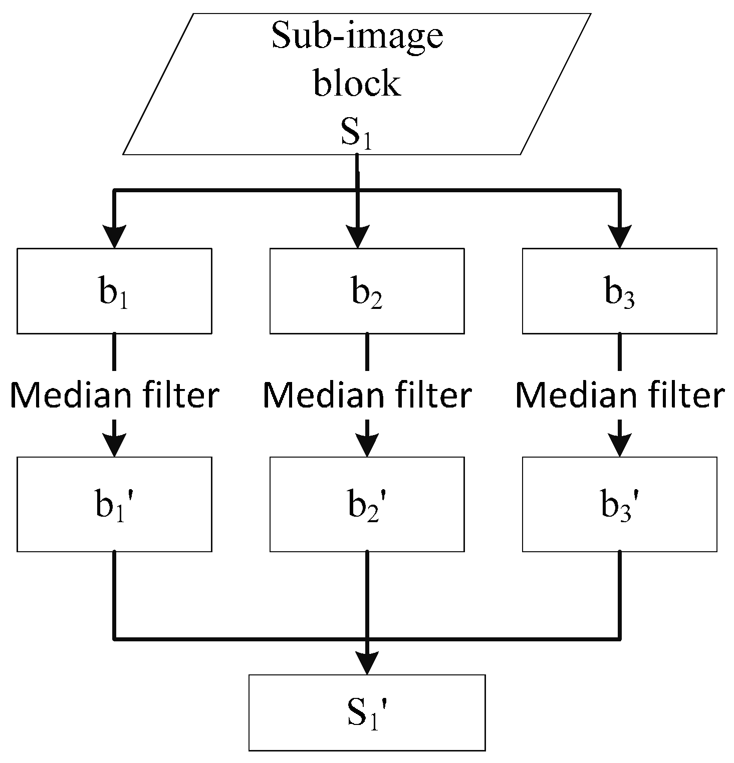
While a scene is being decomposed by the chessboard segmentation method, an image scene is split into numerous sub-image blocks. In this step, each entire sub-image block will be processed by a median filter to remove noise. The median filter algorithm replaces the pixel value with the median of the neighboring pixels. The pattern of neighbors is called the “window,” which slides over the entire sub-image block pixel by pixel, and the size of the window is defined as
. As shown in
Figure 4, the bands (
,
and
) of each sub-image block are processed by median filter, and the result of this process (
,
and
) is fused together as
.
Notably, the processing method for a sub-image block is not limited to a median filter. In general, a spatial feature extraction approach, such as a morphology profile (MP) [
41,
42], can also be used. MP is an effective and classical approach for extracting the spatial information of a VHR image; morphological opening and closing operators are used in order to isolate bright (opening) and dark (closing) structures in the images. Thus, in the following experiments, the proposed system coupled with the MP will also be investigated extensively.
2.3. Sub-Image Block Classification Using a Supervised Classifier
In this section, a training set was selected randomly from the whole image scene in a manual manner and a supervised classifier is adopted to achieve each sub-image block classification. On one hand, from the view of visual cognition, the complexity of the image scene is reduced by the OSSD. On the other hand, from the view of the previous demonstration (
Figure 1), for a pre-given training sample and a supervised model (such as an SVM classifier), it can be found that it is more difficult to classify a larger sub-image block than that of a smaller sub-image block. In theory, it is difficult to evaluate the ability of a supervised classifier for different size testing image-blocks with a pre-given training sample. The classification accuracies not only relate to the distribution of testing datasets and training sample, they also have a strong correlation with the separability of the data and the ability of classifier. Therefore, we try to investigate the effectiveness and feasibility of the proposed OSSD-based approach by experimental comparisons.
3. Experimental Section
In this section, two VHR remote sensing images are used to validate the effectiveness and adaptability of the proposed system for improving the classification performance. Three parts are designed to achieve this purpose. In the first part, the study area is well described. In the second part, two experiments are set up, and the parameter settings are detailed. Finally, the results of the two experiments are given.
3.1. Datasets
Two real VHR remote sensing images are used to assess the effectiveness and adaptability of the proposed system.
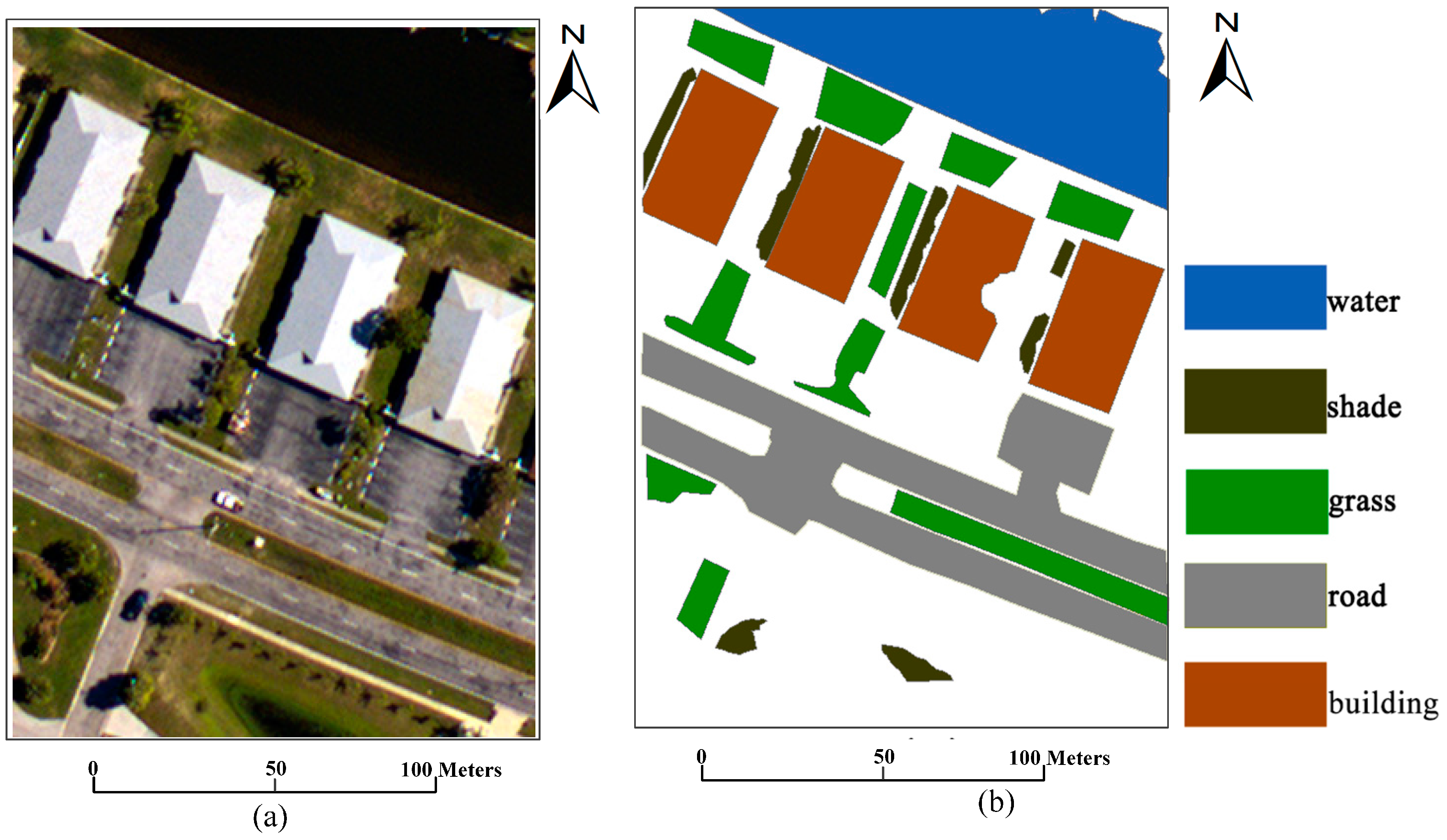
The first image is an aerial image, which is acquired by an airborne ADS80 sensor, as shown in
Figure 5. The relative flying height is approximately 3000 m, and the spatial resolution is 0.32 m. This aerial image is used to compare the accuracy obtained by the proposed OSSD-based classification system with that of without OSSD. The image is classified into five classes, namely, water, shade, grass, road, and building.
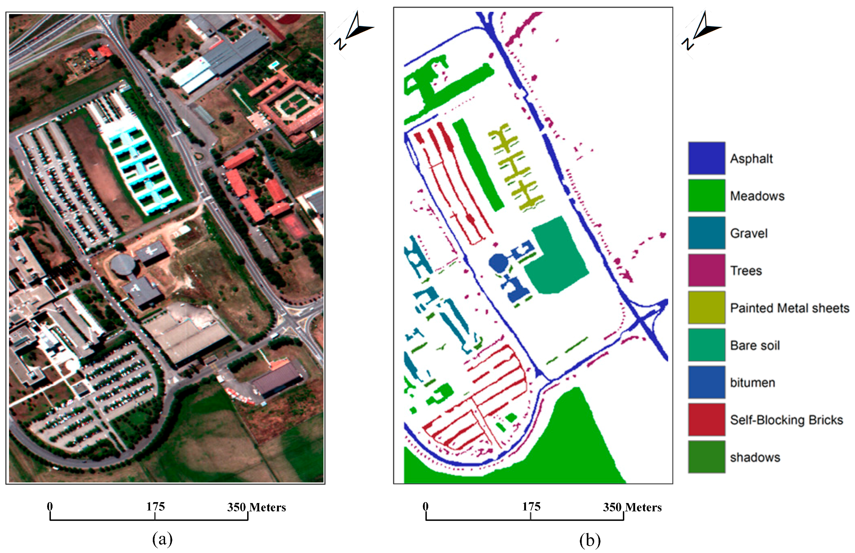
The second dataset is for an image acquired by the ROSIS-03 sensor, which covers the area of Pavia University, north Italy. The original dataset is 610 × 340 pixels with 115 spectral bands, with a spatial resolution of 1.3 m. A false color composite of the image with channels 60, 27, and 17 for red, green, and blue, respectively, is adopted here for our experiment, and the false color image is shown in
Figure 6a. The following nine classes of interest were considered: trees, asphalt, bitumen, gravel, painted metal sheets, shadows, bricks, meadows, and soil. The ground reference map is shown in
Figure 6b.
For both datasets, classification is challenging because of the very high spatial resolution, which is 1.3 m or higher. Only three bands are used as the false color image for each experiment. In addition, as shown in the scene of each image, roads, buildings, water, and shade may be confused with one another. Hence, uncertainties may be engendered during land cover classification.
3.2. Experimental Setup and Parameter Settings
On the basis of the two VHR remote sensing images shown above, the accuracy and adaptability of the proposed OSSD-based classification system are investigated through the following two experimental setups.
The first experiment aims to evaluate the classification accuracies obtained by the proposed OSSD-based system and that of without OSSD processing. Training samples and reference data are collected for the following comparisons. The number of training samples and the reference data are shown in
Table 1. The following four tests are designed: (1) the original test, in which the aerial image is classified without any image processing; (2) a median filter (MedF) test, in which the image is classified on the basis of median filter processing with a 3 × 3 window; (3) an OSSD-based test, in which the image is decomposed by chessboard segmentation, and each sub-image block is classified respectively by the supervised classifier; and (4) the MedF + OSSD test, in which the image is classified through the proposed OSSD-based system. In all the tests, the object size (
) is equal to 90 for the chessboard algorithm. Then, to ensure a fair comparison, the median filter with a 3 × 3 window was also used to process each sub-image block. The above tests were performed based on the same training and reference pixels to ensure fairness.
Adaptability is investigated with four different supervised classifiers, namely, K-nearest neighbor (KNN) [
43], naive Bayes classifier (NBC) [
44], maximum likelihood classifier (MLC) [
45], and SVM [
46], in the above comparison tests. KNN is a non-parametric method used for classification and regression. NBC is a simple probabilistic classifier based on the use of Bayes’ theorem with strong (naive) independence assumptions between the features. MLC depends on the maximum likelihood estimation for each class. The SVM classifier with RBF kernel function and parameters is set by five-fold cross-validation.
OSSD coupled with the spatial feature extraction-MP approach is also investigated in this experiment. A structuring element with a disk shape and a size of 5 × 5 is used to extract structural information in the experiment. The image was first processed by OSSD with a parameter O = 70. Then, each sub-image block is processed by MP instead of a median filter. The processed result is used for classification.
The second experiment: This experiment has two objectives. First, similar to the first experiment, it aims to test the effectiveness of the proposed system. Second, it aims to explore the relationship between parameters and classification accuracies. In this experiment, for the study area of the Pavia University image, training samples were selected randomly, and the reference data are detailed in
Table 2. To achieve these objectives, this experiment is designed as follows:
(1) Classification based on the proposed OSSD-based system is compared with that without OSSD. In addition, the proposed system is also compared with OSSD without any image processing.
(2) The sensitivity of the parameters, including the object size () and the radius () of the median filter, is investigated. The experimental approach incorporated one varied parameter, and the other parameters are constant. The details are shown in the experimental results section.
3.3. Experimental Results
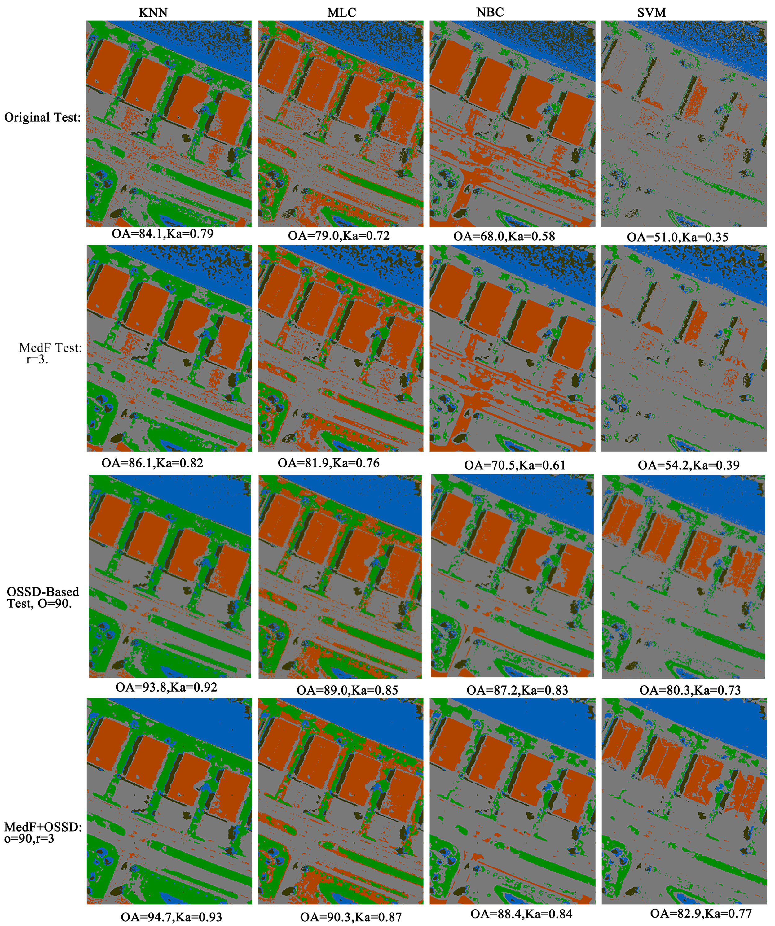
Experiments on the aerial image: The classification results of the four tests for the aerial image are compared in
Figure 7. The results of each test are detailed as follows.
In the original test, the aerial image was directly classified by KNN, MLC, NBC, and SVM. As shown in the first column of
Figure 6, salt-and-pepper noise is observed in each classified map, and the highest accuracy is obtained by KNN. The overall accuracy (OA) for KNN is 84.1%, whereas the kappa coefficient (Ka) is 0.79.
In the MedF-test, the aerial image was classified on the basis of median filter processing. The radius (r) is given as 3 × 3. Compared with the accuracy achieved in the original test, the accuracy of each classifier is improved by approximately 3%, and the noise in the classification map was more or less eliminated.
Further, in the OSSD + MedF test, the proposed OSSD-based system is applied to classify the aerial image. The results indicate that the classification performance achieved by the proposed system is evidently improved for each supervised classifier. The highest accuracy was achieved by the proposed system in terms of the four comparisons with different classifiers. Furthermore, the accuracy of each specific class based on the classifier KNN was also considered in the comparison, as shown in
Table 3. Notably, the classification accuracies of water and grass are obviously improved. The classification accuracy of roads increased from 84.3% to 96.3%.
Finally, another test was adopted for MP. This test investigated the effectiveness of the proposed OSSD coupled with a spatial feature extraction MP, and a disk-shaped structural element with a size of 5 × 5 is employed for MP. The results are shown in
Table 4. The comparison among each result of the original test, MP, and MP + OSSD test indicates that the OA, average accuracy (AA), and Ka are improved when the proposed OSSD is employed for the KNN supervised classifier.
Experiments on the Pavia University Image: In this experiment, the effectiveness of the proposed system was evaluated by comparing the different classification methods for the Pavia University image. Then, the different values for the parameters of the proposed system were tested to detect their influence on the system. The number of training and test pixels in each class is listed in
Table 2, and the available reference data are shown in
Figure 6b. Details about this experiment are given below.
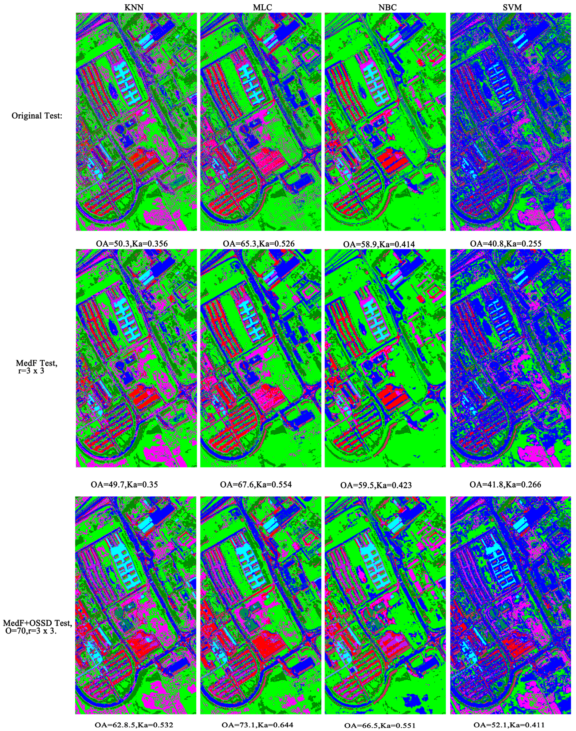
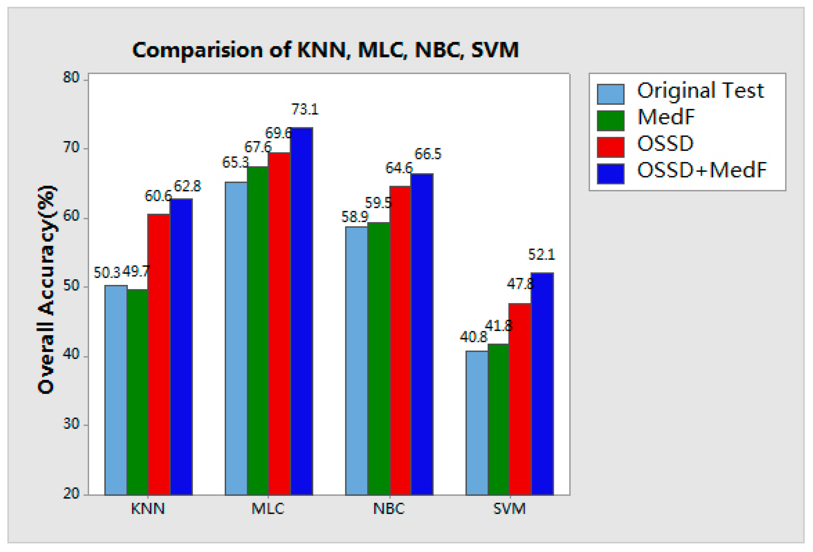
Classification maps acquired by different methods are grouped into four tests and, similar to the first experiment, four supervised classifiers are used, namely, KNN, MLC, NBC, and SVM. As shown in
Figure 8, the original test obtains classification without any scene decomposition or image processing; the MedF test provides the result of the Pavia University image filtered by a median filter with
r = 3. Compared with the original classification, the image scene is decomposed with
O = 70, and the accuracy is improved from 50.3% to 60.6% for KNN. Finally, the OSSD + MedF test shows the results of our proposed approach with parameter settings of
O = 70 and
r = 3.
Specific classes of the four tests according to the KNN classifier were also assessed, as shown in
Table 5. This table, original test and MedF test demonstrated similar accuracies, and the proposed approach for OSSD-based or OSSD + MedF test improved the classification accuracy of most classes. In particular, bitumen and self-blocking bricks were improved by approximately 75% and 51%, respectively. This result was obtained because, compared with their neighboring targets, these classes were more easily identified in a limited spatial range of a single sub-image block by using OSSD processing.
4. Discussion
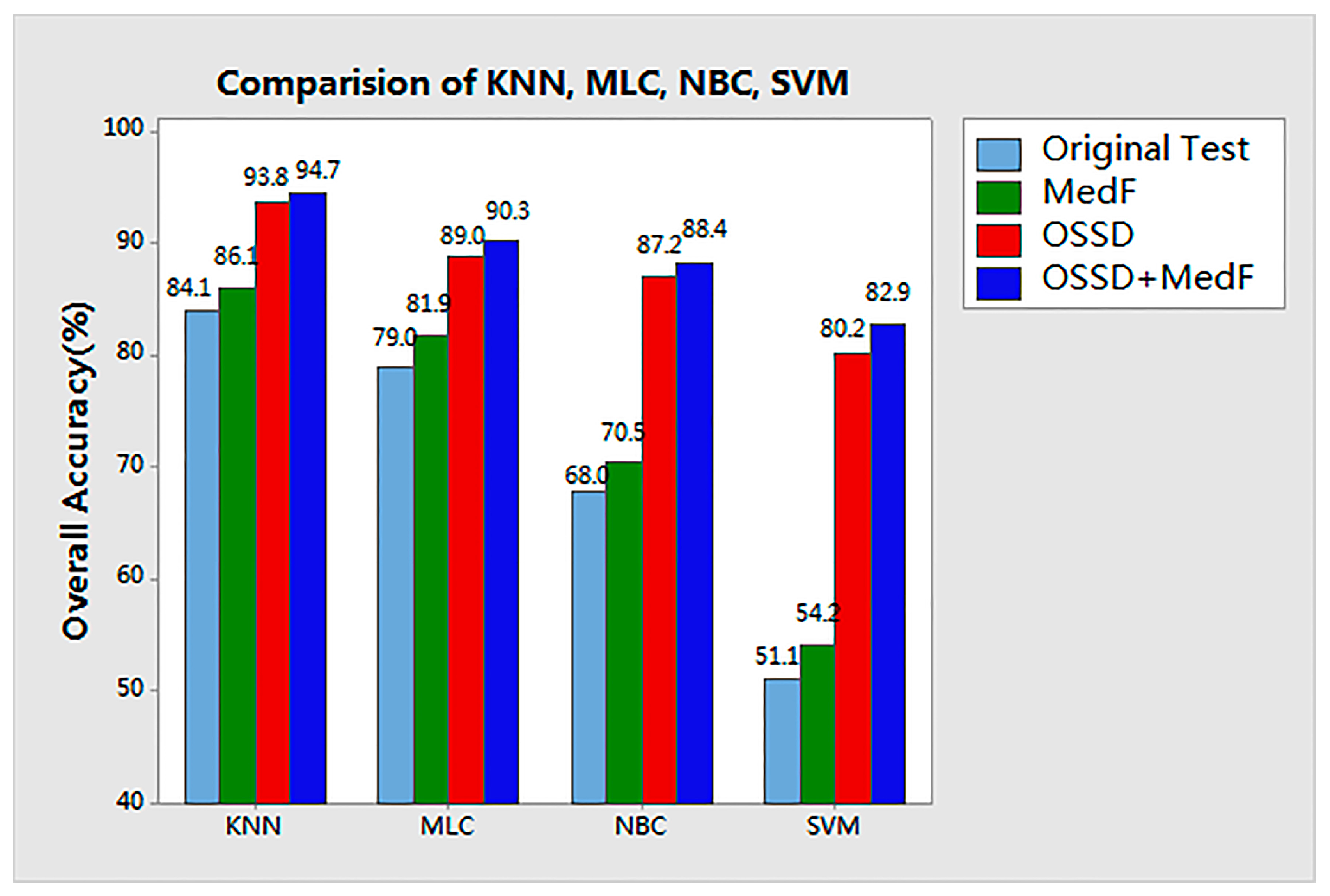
Discussion of Experiment 1: Compared with the results of raw classification, as shown in
Figure 9, while the original image is decomposed and each sub-image block is classified respectively, it can be found that the classification accuracy is notably improved by the decomposition of the image scene.
Notably, in the first experimental results, ground objects with a large scale, such as water, grass, and roads, can be identified with a higher accuracy when OSSD is integrated with MP. However, some smaller and regular-shaped ground objects, such as shade and buildings, exhibited poorer accuracy because their spatial features (such as shape and structure) may be destroyed when OSSD processing is adopted.
Discussion of Experiment 2: A comparison among the results of the four tests on the Pavia University image, as shown in
Figure 10, shows that the classification performance of each supervised classifier in terms of accuracy is improved by the proposed OSSD-based system. The OA of the KNN classifier in particular exhibited an improvement of approximately 12.4%, while OSSD is adopted to decompose the complexity of the image content. MLC, NBC, and SVM all achieved an obvious improvement in terms of OA when OSSD is employed.
Furthermore, the different values for the two parameters, namely, object size (
O) and filter radius (
r), of the proposed system were investigated in this experiment. The training set (
Table 2) and the four classifiers (KNN, MLC, NBC, and SVM) are also employed for this evaluation.
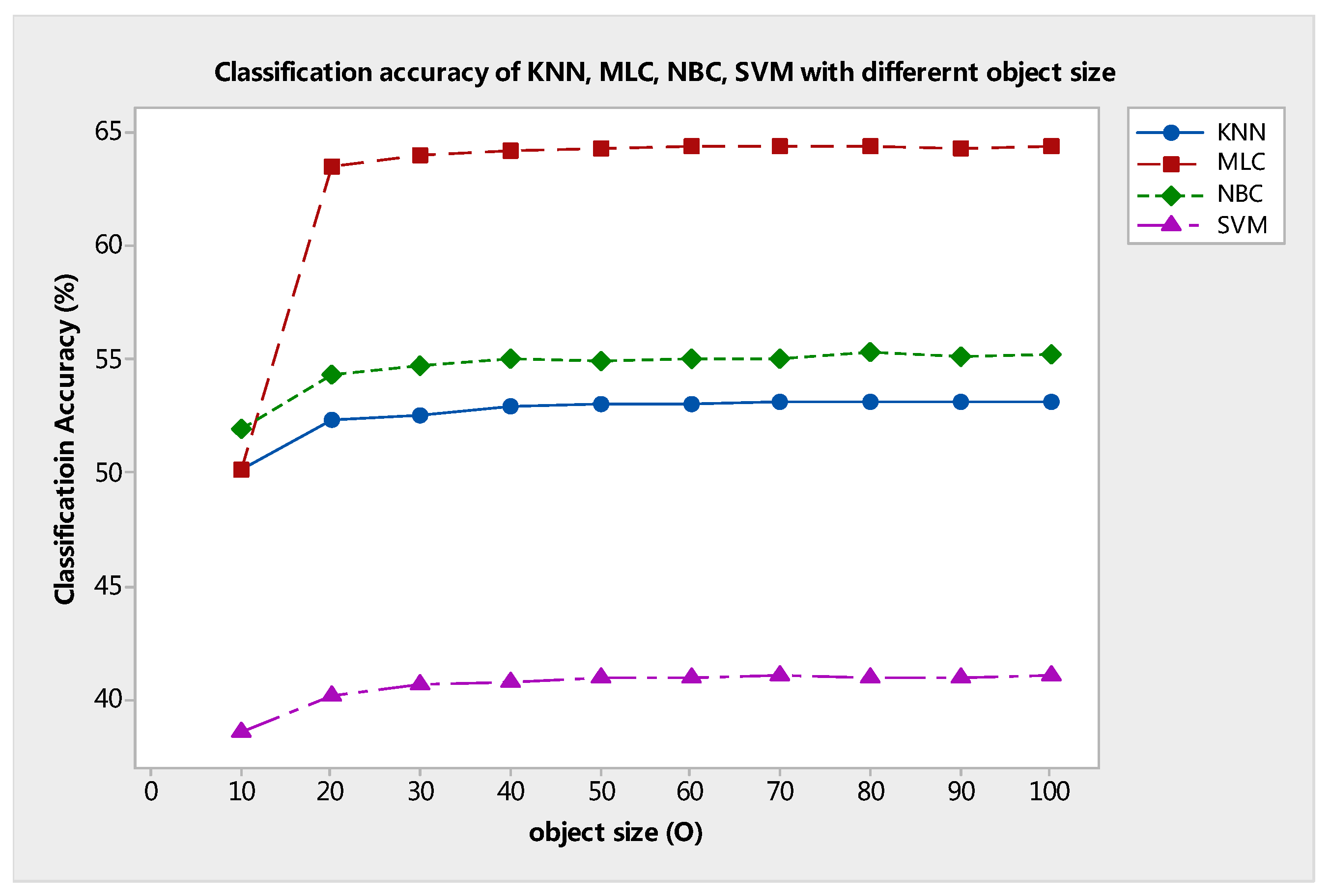
As discussed above, object size (
O) is a parameter of chessboard segmentation. This parameter also indicates the observational scene scale of the proposed system as prepared for the classifier. As mentioned in methodology section A, when the value of
O increases, the larger observational scene scale image block will be extracted from the scene of the image through chessboard segmentation. Therefore, the value of
O is larger, and fewer sub-image blocks will be produced through chessboard segmentation. The classification results with different
O values are shown in
Figure 11. At a fixed median filter radius of
r = 3 × 3, the OA curve grows almost to the horizontal level as
O increases from 10 to 20. Moreover, the classification accuracies of each classifier also increase. However, the curve does not increase with the increment of
O. In fact, the curve gradually reaches a stable trend and remains above 62% (KNN), 72% (MLC), 66% (NBC), and 52% (SVM), despite the wide range of
O from 30 to 100. This test indicates that, if the value of
O is small, then to a certain extent the proposed OSSD-based system cannot work effectively. This result occurs because if a smaller scene covers a single class, then it cannot provide sufficient information for distinguishing between classes.
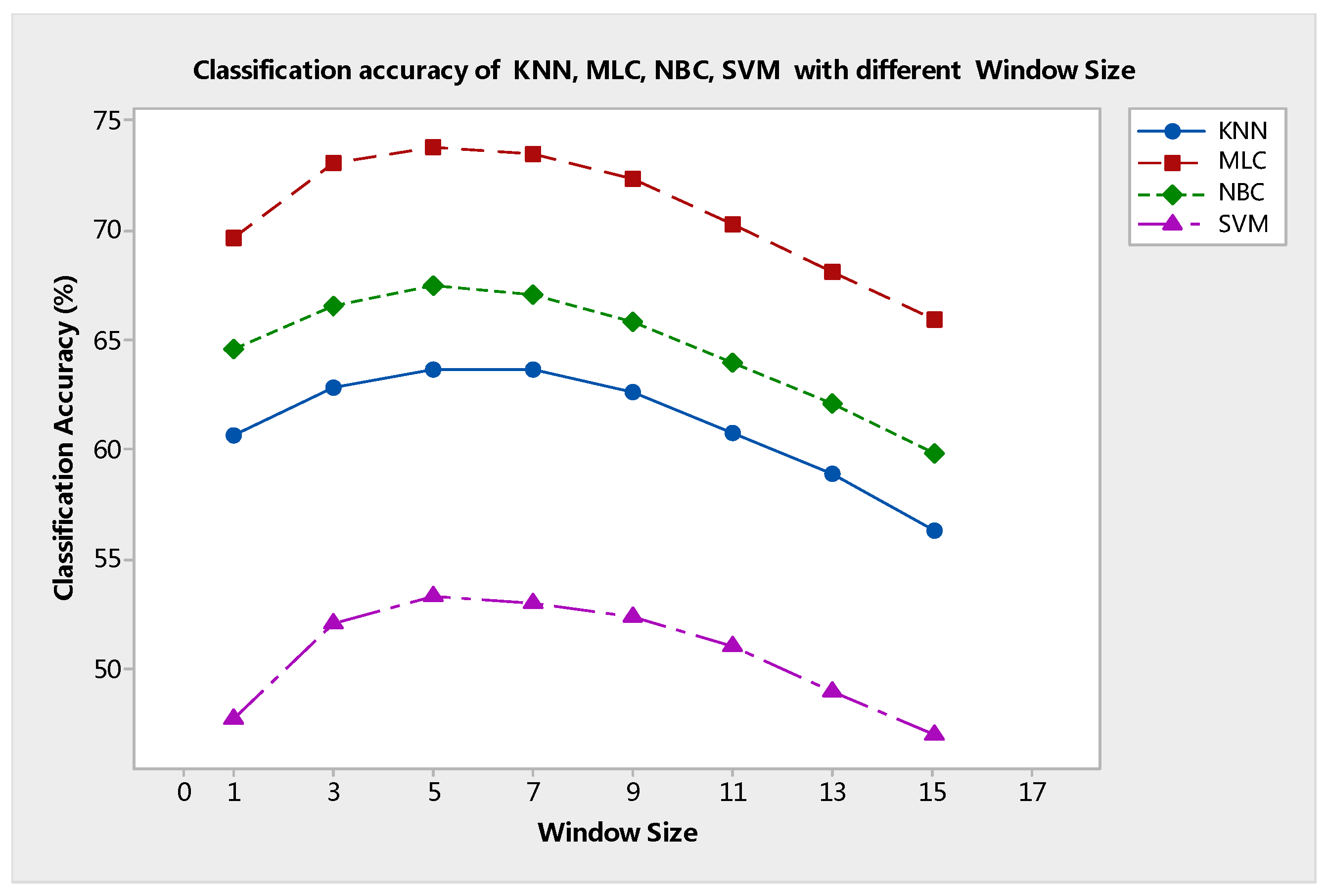
Next, the parameter
r indicates the window size for the median filter processing of every sub-image block. The relationship between OA and
r is shown in
Figure 12. This figure shows that the value of
O was fixed at 90. When the value of
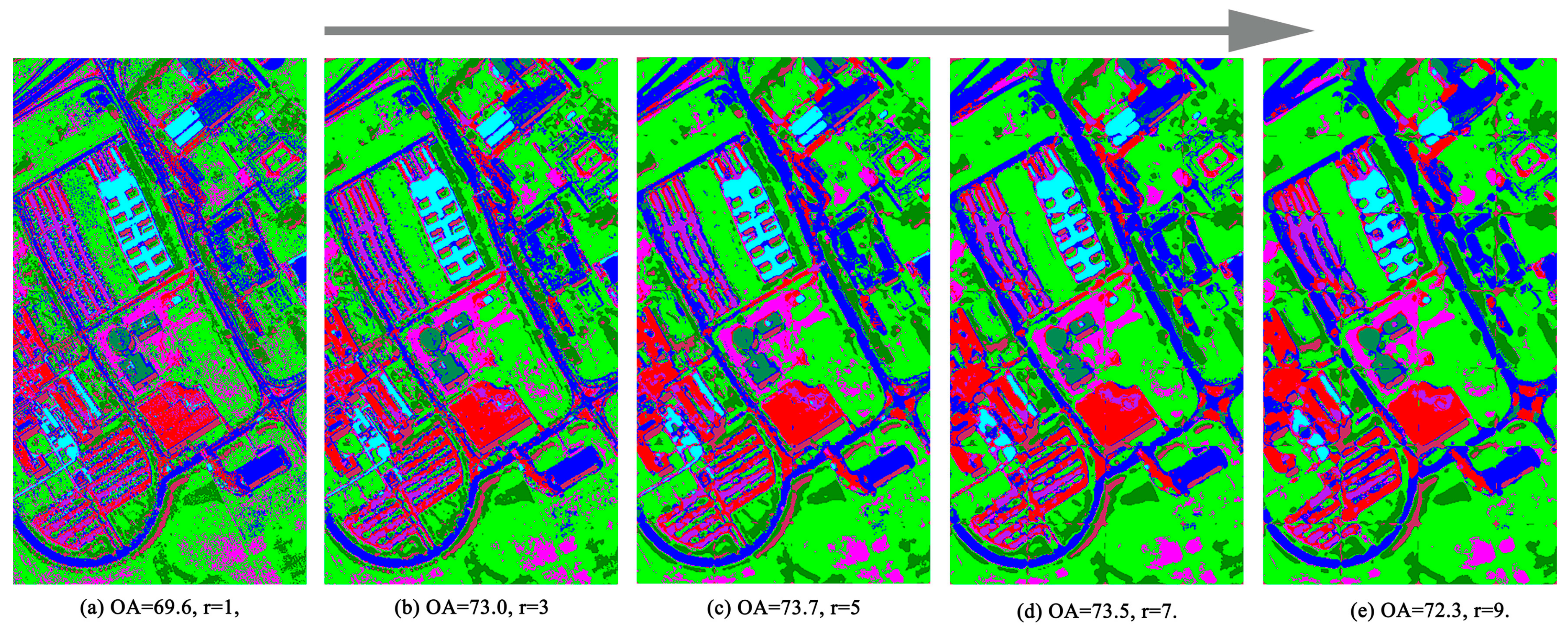
r was varied from 1 to 5, the accuracy gradually escalated to the maximum value. Then, OA declined successively to the minimum when the value of
r increased from 5 to 15. With the increase in window size, sufficient spatial information is considered, and the processing effect of the median filter reaches the optimum. However, an overly large
r value will excessively remove the noise and blur the edge between different objects. Classification map comparisons based on the different values of
r also reveal this fact, as seen in
Figure 13.
Based on the two experimental discussions, it can be seen that the SVM classifier exhibits lower performance compared to the kNN ones in the proposed OSSD method, especially in the Pavia University image scene. This is owing to two aspects: (i) the training size of the Pavia University image is very small, with the training size being only 541 pixels, thus only 1.26% of the total ground truth 42,676 pixels; (ii) when the given image is decomposed into smaller sub-blocks, the number of training/testing samples contained by them is very small, which leads to insufficient learning of the respective classifiers. Therefore, one limitation of the proposed OSSD method is that accuracy depends on the decomposition scale (object size “O”) and each obtained block should contain a few training samples for proper learning of the respective classifiers.
5. Conclusions
In this paper, the relationship between the decomposition of image scene and classification accuracies has been investigated, and a generalized OSSD-based system has been proposed. The proposed system utilized OSSD to limit the spatial range of an image and reduce the complexity of the image content to improve the classification performance. The accuracies of the supervised classifier can be improved by the OSSD-based framework. Experiments were carried out on two real VHR remote sensing images. The results of the experiments showed the effectiveness and feasibility of the proposed OSSD method in improving the classification performance. Moreover, the proposed method has demonstrated several advantages, as is shown in the following:
(1) Our proposed OSSD-based system provides a generalized approach to improving the performance of classifiers. Furthermore, it can be generally applied to many supervised classifiers, because the proposed system presents no a priori constraints and is also data independent. Therefore, our proposed approach has more potential applications in VHR imagery processing and analysis.
(2) With respect to the experimental results, it reveals the fact that land cover classification accuracy can be improved through image scene decomposition. In addition, when OSSD is employed or coupled with an image filter or a feature extraction approach, an overall accuracy and kappa coefficient higher than that without OSSD processing can also be obtained. Therefore, the proposed OSSD-based system proves that the observational scene scale needs to be considered in the classification of VHR images.
With the development of remote sensing technology, a large amount of VHR images can be acquired conveniently, with land cover classification referring to the surface cover on the ground, whether it be vegetation, urban infrastructure, water, bare soil, or other. Identifying, delineating, and mapping land cover is important for global monitoring studies, resource management, and planning activities. Therefore, a generalized and simple classification system plays an important role in practical application.
This study provides a simple and effective strategy to improve VHR image classification accuracy. From the current experiments, it has been noted that the number and size of sub-blocks should be determined according to the class content variability in the terrain. A segmentation method should be chosen to delineate the blocks spatially. However, the class content of a sub-block is uncertain and unknown before classification. In future research, an extensive study of this will be conducted. In addition, the theory of the proposed OSSD-based system will be investigated extensively in other remote sensing applications and image scenes, such as for SAR images or forest image scenes.


