Article

A Case Study of Land-Surface-Temperature Impact from Large-Scale Deployment of Wind Farms in China from Guazhou

1
Center for Earth System Science, Tsinghua University, Beijing 100084, China
2
Public Meteorological Service Center of CMA, Beijing 100081, China
3
National Climate Center, Beijing 100081, China
*
Author to whom correspondence should be addressed.
Remote Sens. 2016, 8(10), 790; https://doi.org/10.3390/rs8100790
Submission received: 13 April 2016 / Revised: 9 September 2016 / Accepted: 19 September 2016 / Published: 23 September 2016
(This article belongs to the Special Issue Remote Sensing of Wind Energy)

Abstract

:
The wind industry in China has experienced a rapid expansion of capacity after 2009, especially in northwestern China, where the China’s first 10 GW-level wind power project is located. Based on the analysis from Moderate Resolution Imaging Spectroradiometer (MODIS) land surface temperature (LST) data for period of 2005–2012, the potential LST impacts from the large-scale wind farms in northwestern China’s Guazhou are investigated in this paper. It shows the noticeable nighttime warming trends on LST over the wind farm areas relative to the nearby non-wind-farm regions in Guazhou and that the nighttime LST warming is strongest in summer (0.51 °C/8 years), followed by autumn (0.48 °C/8 years) and weakest in winter (0.38 °C/8 years) with no warming trend observed in spring. Meanwhile, the quantitative comparison results firstly indicate that the nighttime LST warming from wind farm areas are less than those from the urban areas in this work.

Graphical Abstract

1. Introduction

Although the wind power installed capacity in China was significantly below the potential by the end of 2007 [1], large-scale wind farms are being built at a rapid rate in recent years, especially over the barren Gobi Desert in northwestern China’s Gansu Province. Gaining the advantages of the abundant wind resources there, the ground-breaking ceremony of China’s first 10 GW-level wind power project, namely Jiuquan Wind Power Base, took place on 8 August 2009 [2]. Since then, the capacity of the wind farms in Guazhou known as the “World Wind Library” expanded dramatically. Records show that the installed wind capacity in Guazhou hit 1.12 GW at the end of 2009, 3.0 GW at August 2010, 3.8 GW by the end of 2010 [3,4,5,6], and 4.0 GW at May 2013 [7] with a relatively low expansion speed from 2011 to 2012.
Since the wind turbines convert wind’s kinetic energy into electricity, some efforts have been dedicated to the impacts from the installation and operation phases of wind farms on local climate. Wind turbines could modify the surface-atmosphere exchanges by increasing surface roughness [8,9,10], changing the stability of atmospheric boundary layer (ABL) [11], enhancing turbulence in the rotor wakes [12,13], and interrupting the low-level-jet in stable ABL [14]. A few studies show that the large-scale deployment of wind farms alters the local temperature by up to a few degrees [10,13,15,16,17], reduces precipitation by up to 20% [18], and even mitigates extreme weather [19]. These studies are basically based on limited observation analysis [13,16,20] or model simulations [12,21,22,23]. However, due to the lack of observations, the effects of wind farms are usually parameterized into numerical models by explicitly increasing either surface roughness length or turbulence kinetic energy [24] and the simulating results from these models do not always agree owing to the model or region adopted [25,26], especially the parameterization model of the wind farm effects. Evidently, more in-depth analysis about the wind farm impacts from observations should be strengthened to further the understanding about this question.
Regarding the possible impacts of wind farms on surface temperature, to date only a few studies have used the observed data from operational wind farms, such as the measurements in California [13] and in the Midwestern US [17]. The warming effect from wind farms at night was firstly revealed and was attributed to the turbulence generated by the rotors enhancing the vertical mixing [13]. In the stable atmosphere when a warm layer overlies a cool layer, enhanced vertical mixing mixes warm air down and cold air up, leading to a warming near the surface [12,13]. Then, in situ observations from a large onshore wind farm show that there is little impact on the potential temperature structure during day, but at night the presence of the wind farm does significantly decrease the vertical gradients of potential temperature, largely by increasing the 2-m temperature [17]. However, the short episode (less than two months) as well as the point measurements limit the representativeness of their results. Therefore, more observational evidence of wind farm effects at larger and longer periods have been presented over Texas [16,24,27] and other regions in USA [11,28] based on satellite remote sensing observations. Using Moderate Resolution Imaging Spectroradiometer (MODIS) data, Zhou et al. [16] presented the first observational evidence for the nighttime warming trend of wind farms on LST over the wind farm area relative to the nearby non-wind farm areas with no warming signal at daytime. The seasonal and diurnal variations of such impacts are examined over Texas and their results consistently showed a nighttime warming during all seasons [24]. The possible contributions to these warming signals are also discussed and examined, e.g., wind speed [24], atmospheric stability, land cover, surface albedo [16], topography [27], and turbulence kinetic energy (TKE) [29]. It is pointed out the seasonal variations of wind speed and the relative ratio of TKE induced by the wind turbines compared to the background TKE should play a key role in explaining the above LST changes detected in USA [16,29].
In China, Guazhou is featured by the continental desert climate with dry and infrequent rain throughout the year. Wind blowing with sands often happens in spring and autumn. Temperature difference varies greatly during a day. The unique funneling terrain from the Qilian Mountain to its south, the Mazong Mountain to its north and the flat Gobi Desert in its center (Figure 1a) gives raise to the abundant wind resources in this area.
Because the wind farms over USA and our study area are built on significantly different topography and climate conditions, the primary question of this study is whether the wind farms in Guazhou would yield results similar to the previous studies by analyzing the MODIS LST data and in situ observations from a meteorological station near the wind farm over the study area. This paper demonstrates that (a) the nighttime warming impacts from wind farms in the previous work are not unique; (b) the nighttime LST warming from wind farms are less than those from the urbanization.

2. Materials and Methods
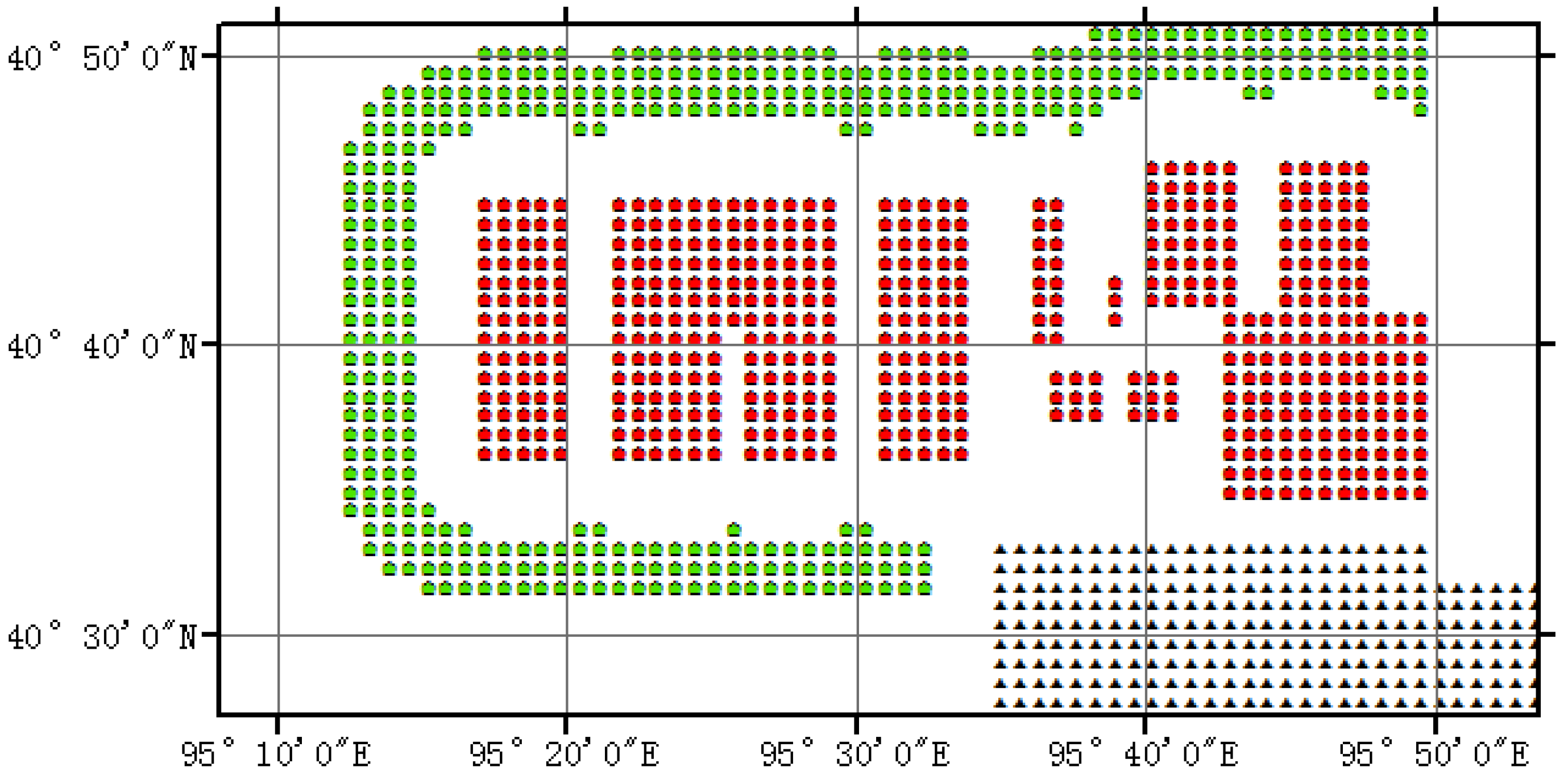
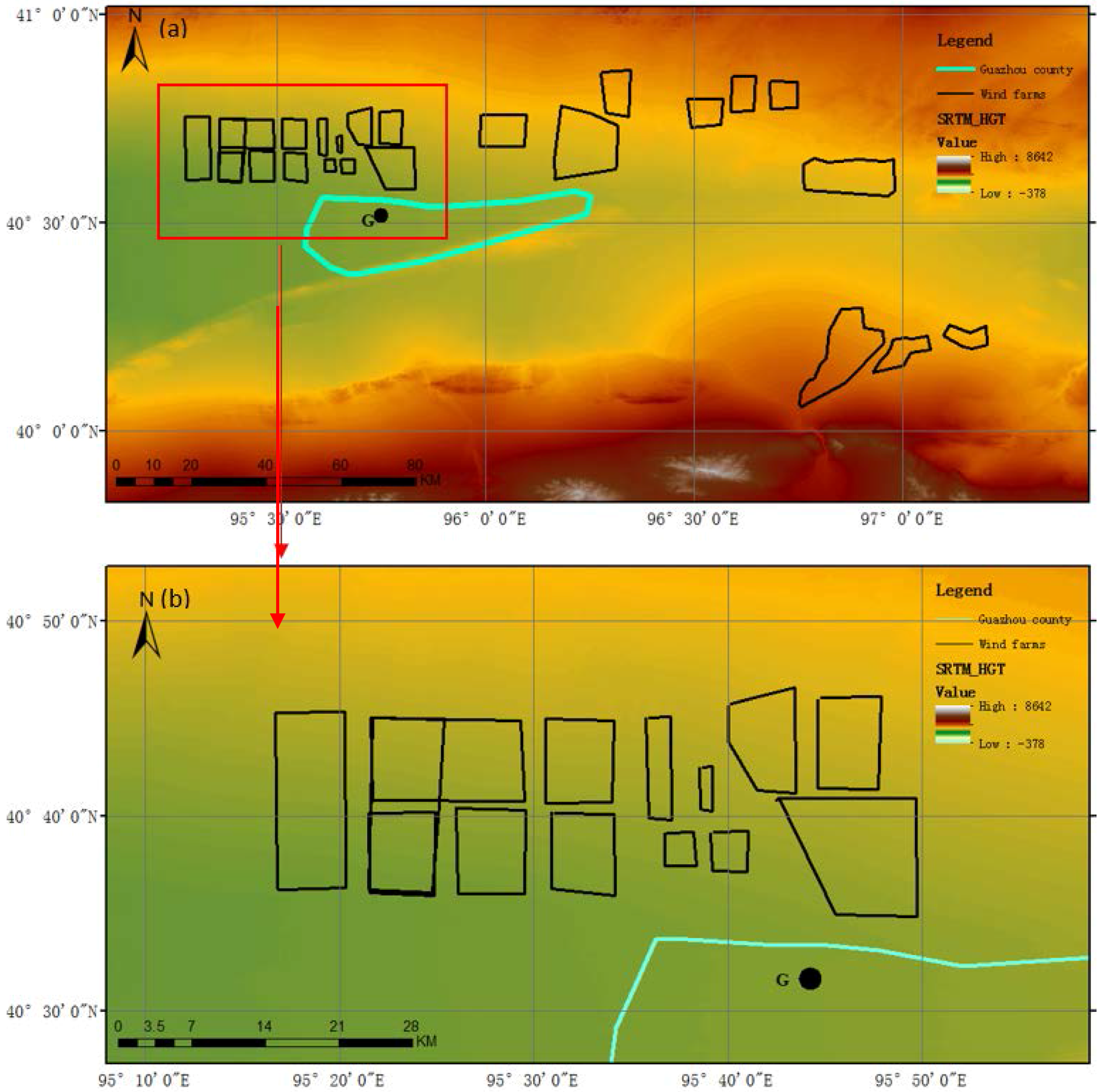
2.1. Study Area

The study area (40.38–40.86°N, 95.08–95.88°E) is located in northwestern China’s Guazhou, as shown in Figure 1. The wind farm locations are verified via Google Earth, where each turbine is visible. In addition to wind farm locations, the center of Guazhou county is also verified and marked by the cyan line in Figure 1. It should be noted that the boundaries of wind farms and Guazhou county are firstly verified through Google Earth and then plotted in Figure 1 by ArcMap. The elevation over this area is defined as the height above the mean sea level and the SRTM digital elevation database at spatial resolutions of ~90 m [30] is used to identify the geographic features of the study area.

2.2. MODIS Data

Eight full years of the Collection 5 MODIS 8-days LST data (MOD11A2 and MYD11A2) [31] and monthly Normalized Difference Vegetation Index (NDVI) data (MOD13A3 and MYD13A3) are used from 2005 through 2012. The two satellites (Terra and Aqua) pass the equator at around local solar time ~10:30 (Terra) and ~13:30 (Aqua) during daytime and ~22:30 (Terra) and ~1:30 (Aqua) at night. Therefore, MODIS Terra and Aqua LST data are combined to produce daytime (averages of local solar time ~10:30 and ~13:30) and nighttime (averages of local solar time ~22:30 and ~1:30) LST in this study.
The spatial resolution of these data is approximately 1 km on a sinusoidal projection, and then re-projected onto a 0.01° resolution grid of pixels using MODIS Re-projection Tool. Because the MODIS thermal infrared signals cannot penetrate thick clouds, there are cloud-contaminated LSTs in the MODIS LST data [32]. The dry and continental climate in Guazhou allows us to use the MODIS LST data mostly for the clear-sky land pixels in the study area. Therefore, the eight-day LST products averaged by 2–8 days daily products are involved in this study, and they represent the best quality retrieval possible from clear-sky conditions with an error better than 1 K [33].

2.3. Meteorological Data

Ground surface temperature (GST) at 0 cm and surface winds at 10 m above the ground for the period 2005–2012 are obtained from an automated meteorological station, located in Guazhou county, which lies in the south of the wind farms (Figure 1, black point G). The meteorological data is provided by the National Meteorological Information Centre of China Meteorological Administration and recorded at six-hour intervals. Here we use these data to create the climatological winds and the inter-annual GST variations at a location closer to the wind farms. This dataset is provided at China Standard Time (CST). The values at 14:00 CST (~13:00 local time in our study area) and 02:00 CST (~01:00 local time in our study area) are chosen to represent the winds at daytime and nighttime, which roughly correspond to the MODIS measurement times.

2.4. Data Processing and Methods

Since MODIS LST contains the background regional inter-annual variability that is unrelated to wind farms, in order to minimize this effect, for each year we firstly subtract the regional mean LST from the original LSTs as proposed by Zhou et al. [24]. This emphasizes the LST spatial variability on the pixel scale. Then the pixel-level anomalies are produced for each month and theses anomalies are aggregated into seasonal ones. For brevity, here we use the following acronyms to represent four different seasons: March-April-May (MAM) is for spring, June-July-August (JJA) for summer, September-October-November (SON) for autumn, and December-January-February (DJF) for winter. Zhou et al. [16] proposed two methods to detect and quantify wind farm impacts on LST between two periods (before and after the wind farms are built). As described in Section 1, the wind turbines in our study area were mostly built from 2009 to the first half year of 2010. In order to avoid the noise from the serious phenomenon of the large scale abandoned wind to brownouts during 2013 over our study area [34], we chose the first three years (2005–2007) of data to represent the case with the least impacts and last three years (the second half year of 2010 to 2012) of data to represent the case with the most likely impacts.
The pixel-level LST differences between the last three years’ mean anomaly values and the first three years’ mean anomaly values are calculated (referred to as method I). Meanwhile, the regional mean LSTs in 2005 and 2012 are similar in our study area (figures not shown here), therefore, they will be used to illustrate the LST change in two individual years in the following section. Note that the resulting warming or cooling rate in method I represents a change relative to the regional mean value.
In order to quantify the impacts of wind farms on LST, the differences between the mean LST value over wind farm pixels (WFM) and that over nearby non-wind farm pixels (NNWF ) for each year (WFM minus NNWF, referred to as method II) are examined. This method has been also used to estimate urban-heat-island effects by comparing the mean LST value over Guazhou county pixels (GZ) and that over NNWF for each year in this paper. Unlike method I, method II does not remove the regional mean value. As showed in Figure 2, pixels with at least one turbine are defined as WFM (in total: 528 pixels in red dots), and NNWF (in total: 448 pixels in green dots) are selected in an area around the WFM that is 3–4 pixels wide and 3–4 pixels away from the nearest WFM. It is noted that the defined NNWF are far enough from the WFM to eliminate downstream impacts [11,29,35]. The black triangles in Figure 2 indicate the pixels (in total: 249 pixels) where the center of Guazhou county is located.

3. Results

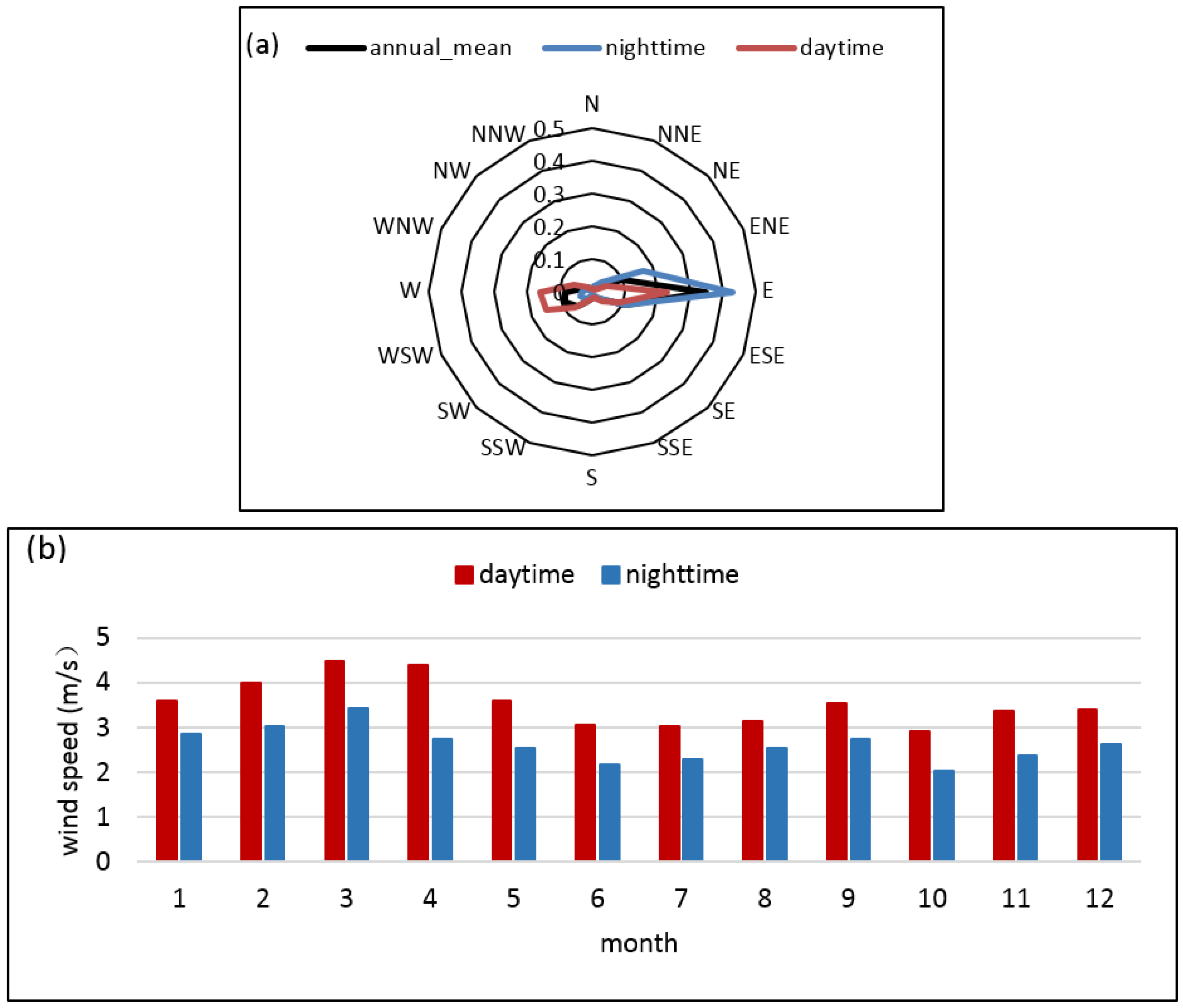
3.1. Climatic Features of Wind in Guazhou

As illustrated in Figure 1a, the funneling terrain in Guazhou has an important effect on the high frequency of easterly winds in this area, especially during nighttime (Figure 3a). As for wind speed in Guazhou, the measurements from the meteorological station show that the wind speeds are stronger at daytime than those at nighttime with a maximum value in spring and a relatively small value in summer for the period 2005–2012 (Figure 3b). These unique climatic features of wind make Guazhou known as the “World Wind Library”.

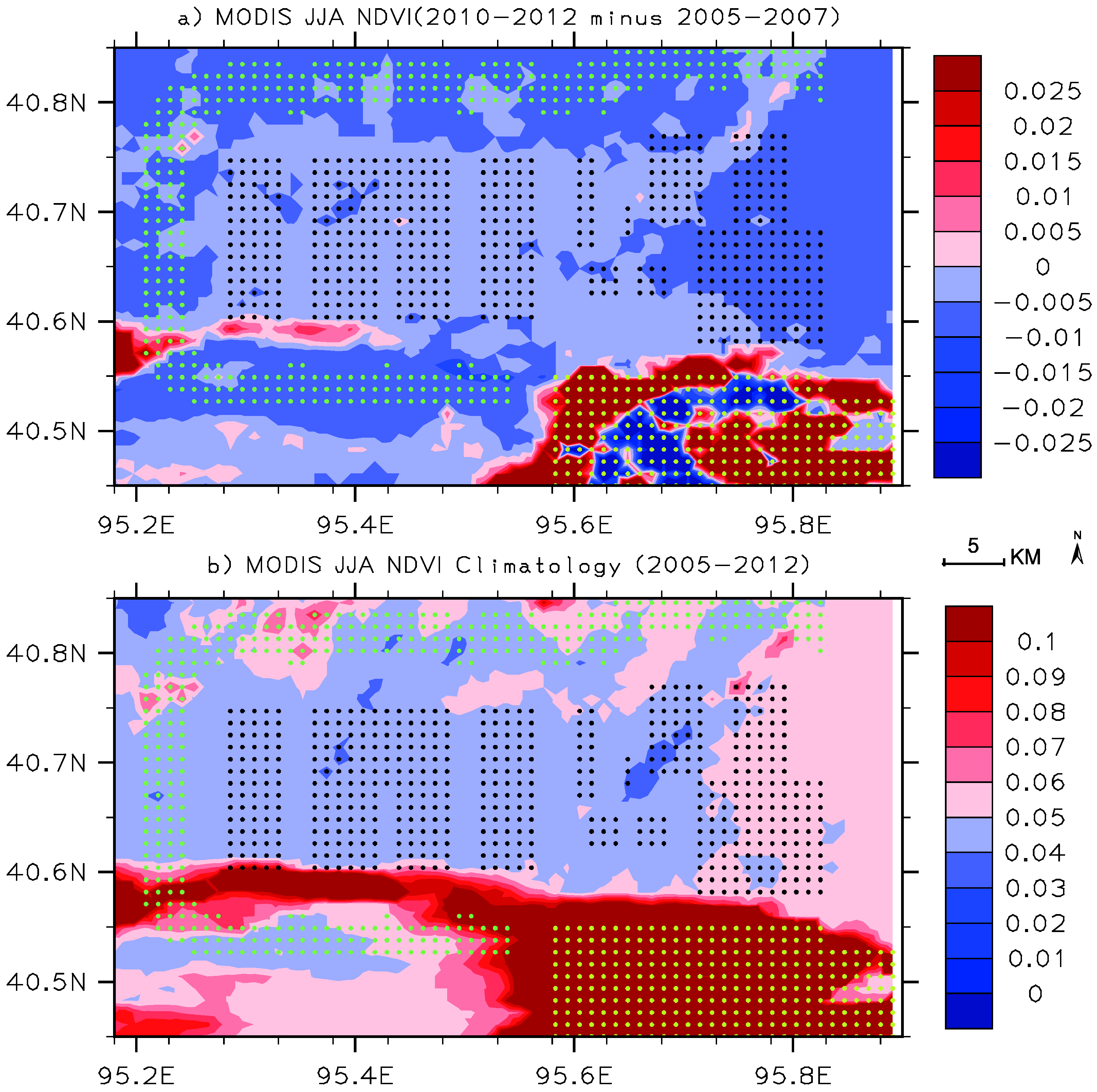
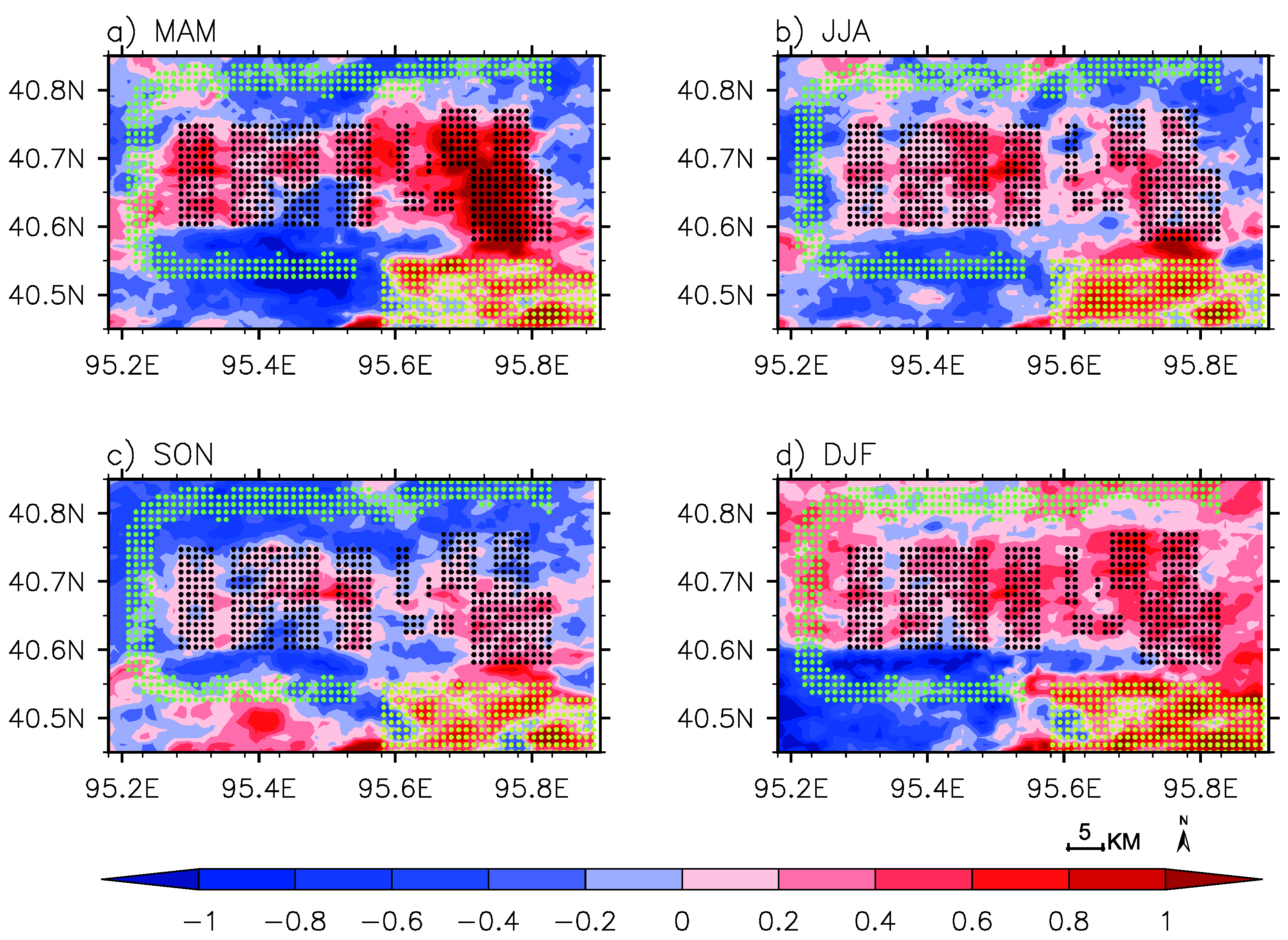
3.2. Spatial Coupling Analysis of LST Changes

In order to detect the spatial LST changes with the wind turbines, the LST anomalies for the pre-turbine period (2005–2007) are subtracted from the LST anomalies for the post-turbine period (the second half year of 2010–2012) and Figure 4 shows the seasonal LST differences for these two periods at nighttime (method I). Similarly, the two individual years, 2005 and 2012, are chosen to illustrate the LST changes in the typical year as well as to demonstrate the effectiveness of the approach (Figure 5). The regional mean value is removed from the LST anomaly difference to highlight the LST changes relative to the regional mean [16]. Therefore, it should be noted that the resulting warming or cooling rate in Figure 4 and Figure 5 represent a change relative to the regional mean value.
In these two figures, the red contours indicate areas where the LST anomaly in post-turbine years is greater than that in the pre-turbine years, while the blue contours are the areas with lower LST anomaly in the post-turbine years. It shows that the LST anomalies over WFM pixels are higher than those over NNWF pixels at nighttime during almost all seasons with the most prominent pattern in summer and the relatively noisy signal in spring (Figure 4). Figure 5 exhibits the similar features at nighttime as Figure 4 but with a larger magnitude. The signal of daytime LST anomalies shows a lot of noise (figures not shown here) and is therefore not included. The noticeable nighttime warming during almost all seasons are likely caused by the wind turbine operation since the spatial warming patterns generally resemble the wind farm layouts to some extent.
In both Figures, there’s an area of strong positive anomalies just the location of Guazhou county indicated by yellow dots. This feature is investigated further, and it is primarily attributed to the local urban heat island effects in Guazhou county, which maintains a high-speed economic development mainly driven by the dramatic expansion of wind power industry [36,37,38,39,40]. The potential LST impacts from wind farm versus Guazhou county will be quantified and compared in the following section. Although there are some WFM pixels characterized by either neutral or negative LST variability, likely due to cloud and aerosol contamination, the averaging methods used here should remove most of the high-frequency noise [24] and could be used to uncover the wind farm impacts.

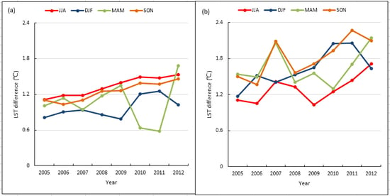
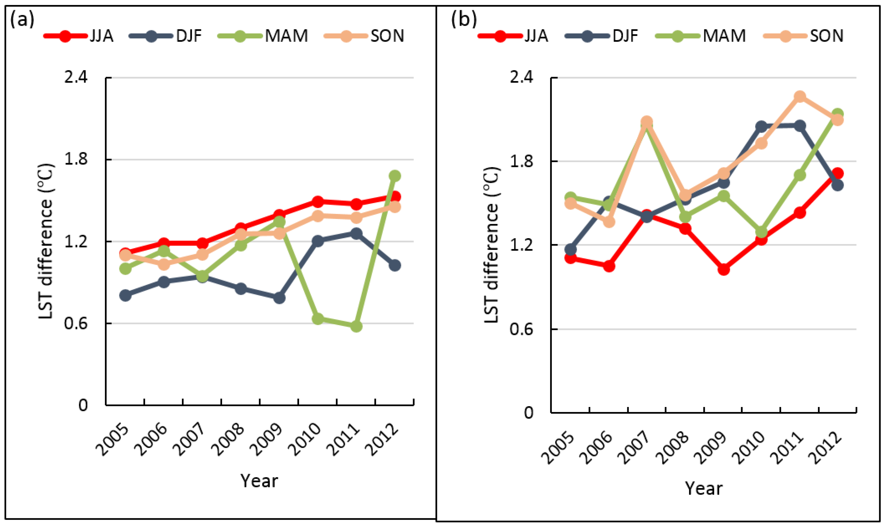
3.3. Temporal Variability of LST Impacts from Wind Farm Versus Guazhou County

As described in Section 2.4, method II is used to examine how the LST differences between WFM and NNWF changes temporally with the development of wind farms as done in Zhou et al. [16]. This method has been also used to estimate urban-heat-island effects by comparing the mean LST value over Guazhou county pixels (GZ) and that over NNWF for each year here. Figure 6 shows the areal mean seasonal time series of LST differences (WFM minus NNWF in Figure 6a; GZ minus NNWF in Figure 6b) from 2005 to 2012. Since the mean height over the WFM pixels (1237.8 m) is lower than that over the NNWF pixels (1293.3 m), the LST differences in Figure 6a start above 0.6 °C before the wind farms are installed. Therefore, the results based on method II here might overestimate the magnitude of LST difference in the individual year, but the total trend is clear.
Despite the strong inter-annual variability, there are clearly warming trends of LST differences during summer, autumn, and winter at nighttime both in Figure 6a,b, which indicate that the construction of wind turbines and the development of urbanization respectively warm the WFM and GZ relative to NNWF at night during these seasons. The total trend is calculated as the linear trend per year estimated using least squares fitting multiplied. The estimated trends are listed in Table 1.
Although there are only eight years of data, method II can be used to quantify the warming changes with time because the correlation coefficient (R) between the linear trend and the observations can be used to tell whether the linear trend value is statistically significant as shown in Table 1. The LSTWFM-NNWF warming trend is found to be the largest in summer (0.51 °C/8 years), followed by autumn (0.48 °C/8 years), and winter (0.38 °C/8 years) at night. The LSTGZ-NNWF holds similar warming trends but with larger magnitudes especially in autumn (0.80 °C/8 years) and winter (0.76 °C/8 years). These warming trends are statistically significant to the results of t-test [41] at 5% confidence level. The larger warming trends of LSTGZ-NNWF compared to LSTWFM-NNWF in our study area present the case that the LST impacts from wind farms are less than those from the urban area (Guazhou county).
However, the LSTWFM-NNWF and LSTGZ-NNWF trends in spring at nighttime and in all seasons at daytime are considered not significant (Table 1). The noisy signal in these issues may suggest that the characteristics of the near-surface boundary layer at spring night and all daytime in Guazhou are not favorable for allowing wind farm and urban impacts to be observed with these methods (further discussion is later provided).
The MODIS LST is the only high quality satellite data that are publicly available and have long time spans covering both day and night times. Although the MODIS data used in this study do contain errors and noise [23], the use of spatial and temporal averaging should largely remove such errors and uncertainties whose remaining residuals cannot accidently create the spatial coupling shown above [16]. Furthermore, the validation results indicate that MODIS LST matches well with the in situ observations near our study area [42,43]. Meanwhile, some of the LST changes could associate with the turbine footprint, such as turbine blades, towers, and access roads et al. However, the footprint area occupies only a small percentage of the total land area of wind farms because inter-turbine spacing is required to maximize its efficiency [16]. Therefore, the warming effect seen in the MODIS over wind farms are very likely due to the development of wind farms.

4. Discussion

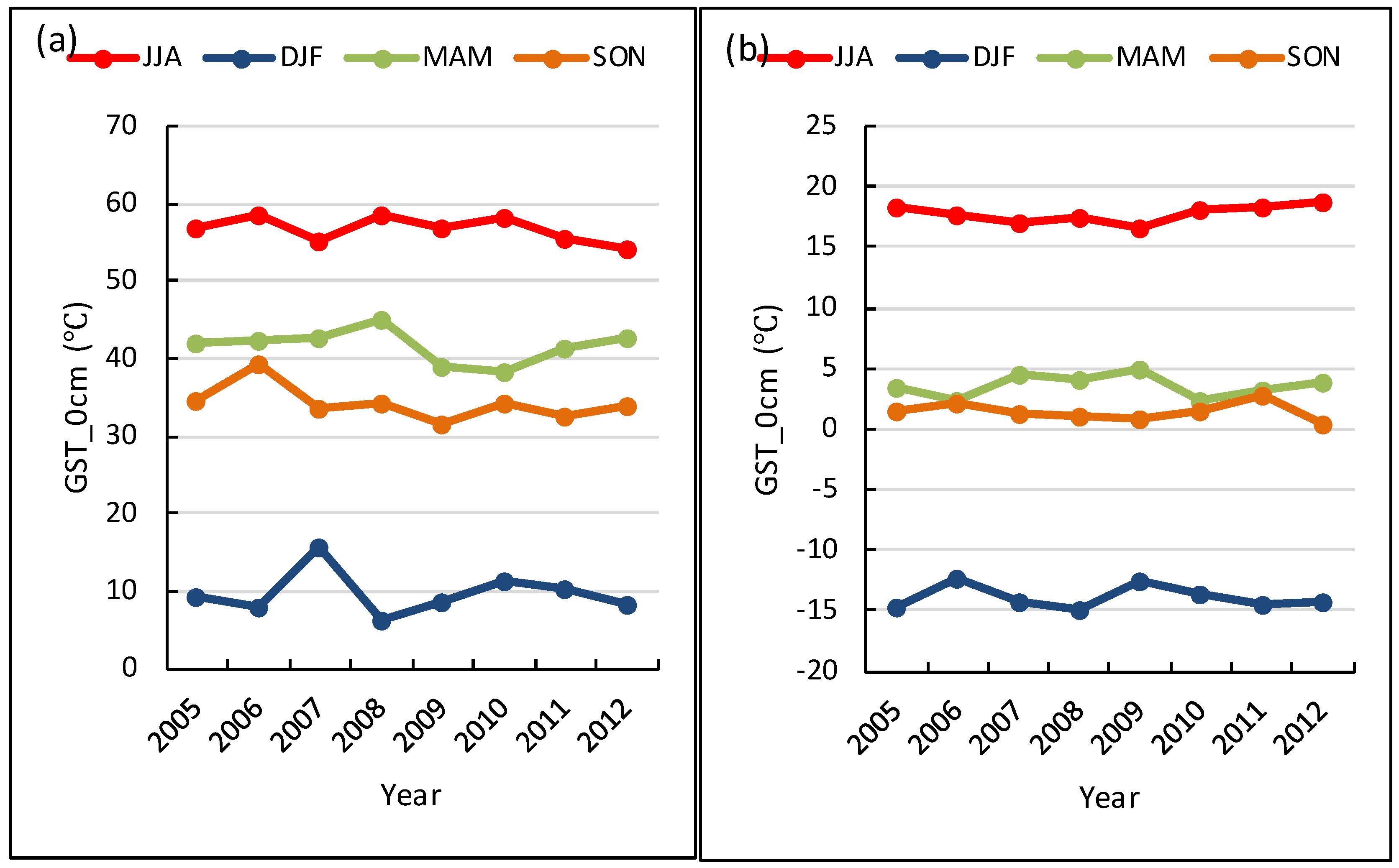
4.1. Inter-Annual Variations of GST Observed in Guazhou

Figure 7 illustrates the inter-annual variability of GST for the period 2005–2012 observed at Guazhou meteorological station. It shows a relatively smooth variation of the GST both at daytime and nighttime (Figure 7a,b). The total trends are calculated as the linear trend per year estimated using least squares fitting multiplied. The estimated trends and the correlation coefficient (R) between the linear trend and the observations show that the trends of GST in Guazhou are not significant both at day and night on the basis of t-test at a 5% confidence level, which indicates a relatively weak background climate signal for this period in our study area. These findings make the results in Section 3 more certain.

4.2. Possible Impacts of Temporal Changes in Land Cover on LST Variability

The above results indicate that there is a warming effect seen by MODIS at nighttime coupled with the wind farms over our study area. Land surface properties can be also modified by the temporal changes in precipitation, soil moisture, and vegetation et al. Here, we use the MODIS vegetation data (NDVI) to quantify possible changes in land surface properties.
We quantify changes in NDVI by examining their spatial patterns as done for LST. It shows that the NDVI changes exhibit no apparent WFM versus NNWF differences and no spatial coupling with the LST changes (Figure 8a versus Figure 4b). Meanwhile, the wind farms in our study area are built on the barren Gobi Desert in northwestern China. The climatology NDVI values on WFM pixels are almost less than 0.05 (Figure 8b). The increased vegetation greenness over GZ pixels is proposed to have a positive contribution to the nighttime warming observed in the urban area (Guazhou county). Compared to their surrounding NNWF pixels, WFM pixels do show negligible decrease in vegetation greenness. On average, the mean absolute NDVI value in 2010–2012 decreased by −0.0038 relative to that in 2005–2007, representing a change of 7.9% of the climatology value 0.048 over the WFM region (Figure 8). Such changes are too small and cannot explain the nighttime warming effects over WFM pixels seen by MODIS.
Given the small size of our study region as well as the approach involved here, the contributions from the incoming radiation and the land surface properties (topography, land-cover type et al.) to the warming impacts are likely been minimized [16]. Based on the reanalysis wind data, Zhou et al. (2012) proposed that the seasonal and diurnal variations in wind speed primarily determine the seasonal variations of the wind farm-induced warming [16]. However, the strongest wind speed in MAM (Figure 3b) cannot explain the noisy wind farm-induced warming in spring (Table 1) observed over this wind farm. Therefore, it is reasonable to assume that other factors may play an important role in this question.
Because of the solar heating at the surface, the daytime ABL is typically unstable and much thicker than the nocturnal ABL. It is expected that the enhanced vertical mixing generated by wind turbine rotors will create a warming effect at nighttime by pulling down warmer near-surface air from higher altitudes [8,12]. The diurnal difference suggests that the wind farm impact is much larger and thus more detectable at nighttime than at daytime. This agrees with the asymmetric day–night differences in the MODIS LST changes observed over the wind farms (Table 1).
Based on the radiosonde observations, recent study finds that the turbine-induced turbulence relative to the background TKE plays an essential role in determining those in the magnitude of LST changes over the wind farms [29]. The strong wind speeds (Figure 3b) and the frequently complex synoptic-scale weather events [12] in spring are more likely to induce strong background TKE, which will mask the turbine-induced turbulence effect and consequently contribute to the noisy warming signals (0.12 °C/8 years) in this season. Further understanding about the complex processes in this question will rely on more and longer observations in the future.
Furthermore, there is a seasonal shift in the spatial coupling between nighttime LST warming and wind farm pixels, especially during autumn and winter (Figure 4c,d). The dominant easterly winds at nighttime during the whole year (Figure 3a) could be an important factor for these shifts in the spatial coupling, as the positive LST anomalies are located primarily in the western pixels near the wind farms.

5. Conclusions

Based on the analysis from MODIS LST data, we further the recent work carried out by Zhou et al. (2012) through investigating the potential LST impacts from the large-scale wind farms in northwestern China’s Guazhou, where the topography and climate conditions are significantly different from those in USA. Our analysis shows significant warming trends at nighttime during summer, autumn, and winter for the period 2005–2012, but no noticeable impact is detected during daytime. In terms of the seasonal magnitude of the warming trend, it shows that the nighttime LST warming is strongest in summer (0.51 °C/8 years), followed by autumn (0.48 °C/8 years), and weakest in winter (0.38 °C/8 years) with no warming trend observed in spring. The nighttime warming trends of LSTWFM-NNWF compared to LSTGZ-NNWF with the magnitude of 0.51–0.80 °C/8 years show that the LST impacts from wind farms are less than those from the urban area.
These warming signals are important for the development of wind project in Guazhou, since the spatial pattern couples well with the geographic layouts of wind turbines, which provides further observational evidence for the WF-induced surface warming at nighttime proposed by Zhou et al. (2012). However, analysis of seasonal variations in wind speed suggest that the seasonal variations in the magnitude of the warming trends in Guazhou do not correspond to the magnitude of wind speeds, which is totally different from the work carried by Zhou et al. (2012) [16]. Further understanding about the complex processes in this question will rely on more and longer observations in the future.
When interpreting our results, it should be noted that (a) the wind turbine itself does not create a net warming of the air, but only transports the heat between different heights in the atmosphere [13]; and (b) the overall warming effect from wind farms reported in this study is local and is small compared to the strong warming effects from the urbanization.

Acknowledgments

The funding for the project “A Study on Climate Effects of Large Scale Construction Program of Wind Farms and Solar PV Plants in China” from the National Natural Science Foundation of China (Grant No. 41475066), the project “Study on the estimation of the mid-high latitude offshore extreme winds based on numerical modeling and spectrum analysis” from the National Natural Science Foundation of China (Grant No. 41605086), the project “Studies on the potential of wind energy and carbon dioxide emission in China” from the Climate Change Special Fund of China Meteorological Administration (Grant No. CCSF201624), and Tsinghua University Initiative Scientific Research Program (Grant No. 20131089357) are kindly acknowledged.

Author Contributions

Rui Chang and Rong Zhu designed and performed the research; Rui Chang and Peng Guo analyzed the data and wrote the manuscript.

Conflicts of Interest

The authors declare no conflict of interest.

References

  1. Wu, C.; Sha, Y.; Gu, W.; Yin, L.; Fang, Z.; Zhang, Y. Trend in China’s wind power. Electricity 2009, 1, 17–24. [Google Scholar]
  2. Li, W.Z. High on Wind Power. In China Today-Explaining China to the World (Special Report on Website). Available online: http://www.chinatoday.com.cn/ctenglish/se/txt/2009-11/26/content_231445.htm (accessed on 13 April 2016).
  3. Li, Z.; Yang, S. “Three Gorges on Land” emerges at Qiuquan: Song of the wind sang in Gobi and renewable energy turned out by rotors. RENMI RIBAO, 8 August 2009. (In Chinese) [Google Scholar]
  4. Li, X. Exploration of large-scale wind power base in Qiuquan. China News, 24 August 2010. (In Chinese) [Google Scholar]
  5. Li, S.; Liu, X. Guazhou’s wind power generating capacity totaled at 15.36 billion degrees. Chinese Wind Energy Industry, 9 June 2013. (In Chinese) [Google Scholar]
  6. Zhang, H. Guazhou’s wind power installed capacity ranks the first in China. Gansu Daily, 23 February 2011. (In Chinese) [Google Scholar]
  7. Zhang, W. Guazhou’s wind power installed capacity has ranked the first in China. Gansu Daily, 9 July 2013. (In Chinese) [Google Scholar]
  8. Barrie, D.B.; Kirk-Davidoff, D.B. Weather response to a large wind turbine array. Atmos. Chem. Phys. 2010, 10, 769–775. [Google Scholar] [CrossRef]
  9. Wang, C.; Prinn, R.G. Potential climatic impacts and reliability of very large-scale wind farms. Atmos. Chem. Phys. 2010, 10, 2053–2061. [Google Scholar] [CrossRef]
  10. Kirk-Davidoff, D.B.; David, W.K. On the climate impact of surface roughness anomalies. J. Atmos. Sci. 2008, 65, 2215–2234. [Google Scholar] [CrossRef]
  11. Slawsky, L.; Zhou, L.; Baidya, R.S.; Xia, G.; Vuille, M.; Harris, R.A. Observed thermal impacts of wind farms over northern illinois. Sensors 2015, 15, 14981–15005. [Google Scholar] [CrossRef] [PubMed]
  12. Baidya, R.S.; Pacala, S.W.; Walko, R.L. Can large wind farms affect local meteorology? J. Geophys. Res. 2004, 109. [Google Scholar] [CrossRef]
  13. Baidya, R.S.; Traiteur, J.J. Impacts of wind farms on surface air temperatures. Proc. Natl. Acad. Sci. USA 2010, 107, 17899–17904. [Google Scholar] [CrossRef] [PubMed]
  14. Bhaganagar, K.; Mithu, D. Implications of stratified atmospheric boundary layer turbulence on the near-wake structure of wind turbines. Energies 2014, 7, 5740–5763. [Google Scholar] [CrossRef]
  15. Keith, D.W.; DeCarolis, J.F.; Denkenberger, D.C.; Donald, H.L.; Sergey, L.M.; Stephen, P.; Philip, J.R. The influence of large-scale wind-power on global climate. Proc. Natl. Acad. Sci. USA 2004, 101, 16115–16120. [Google Scholar] [CrossRef] [PubMed]
  16. Zhou, L.; Tian, Y.; Baidya, R.S.; Thorncroft, C.; Bosart, L.F.; Hu, Y. Impacts of wind farms on land surface temperature. Nat. Clim. Chang. 2012, 2, 539–543. [Google Scholar] [CrossRef]
  17. Smith, C.M.; Barthelmie, R.J.; Pryor, S.C. In situ observations of the influence of a large onshore wind farm on near-surface temperature, turbulence and wind speed profiles. Environ. Res. Lett. 2013, 8. [Google Scholar] [CrossRef]
  18. Fiedler, B.H.; Bukovsky, M.S. The effect of a giant wind farm on precipitation in a regional climate model. Environ. Res. Lett. 2011, 6, 045101. [Google Scholar] [CrossRef]
  19. Jacobson, M.Z.; Cristina, L.A.; Willett, K. Taming hurricanes with arrays of offshore wind turbines. Nat. Clim. Chang. 2014, 4, 195–200. [Google Scholar] [CrossRef]
  20. Rajewski, D.A.; Takle, E.S.; Lundquist, J.K.; Oncley, S.; Prueger, J.H.; Horst, T.W.; Rhodes, M.E.; Pfeiffer, R.; Hatfield, J.L.; Spoth, K.K.; et al. Crop wind energy experiment: Observations of surface-layer, boundary layer, and meso-scale interactions with a wind farm. Am. Meteorol. Soc. 2013, 94, 655–672. [Google Scholar] [CrossRef]
  21. Frandsen, S.T.; Jorgensen, H.E.; Barthelmie, R.; Rathmann, O.; Badger, J.; Hansen, K.; Ott, S.; Rethore, P.E.; Larsen, S.E.; Jensen, L.E. The making of a second generation wind farm efficiency model complex. Wind Energy 2009, 12, 445–458. [Google Scholar] [CrossRef]
  22. Keith, D.; DeCarolis, J.; Denkenberger, D.; Lenschow, D.; Malyshev, S.; Pacala, S.; Rasch, P.J. The influence of large-scale wind power on global climate. Proc. Natl. Acad. Sci. USA 2004, 101, 16115–16120. [Google Scholar] [CrossRef] [PubMed]
  23. Fitch, A.; Olson, J.; Lundquist, J.; Dudhia, J.; Gupta, A.; Michalakes, J.; Barstad, I. Local and mesoscale impacts of wind farms as parameterized in a mesoscale NWP model. Mon. Weather Rev. 2012, 140, 3017–3038. [Google Scholar] [CrossRef]
  24. Zhou, L.; Tian, Y.; Baidya, S.R.; Dai, Y.; Chen, H. Diurnal and seasonal variations of wind farm impacts on land surface temperature over western Texas. Clim. Dyn. 2013, 41, 307–326. [Google Scholar] [CrossRef]
  25. Fitch, A.C.; Olson, J.B.; Lundquist, J.K. Parameterization of wind farms in climate models. J. Clim. 2013, 26, 6439–6458. [Google Scholar] [CrossRef]
  26. Lu, H.; Fernando, P.A. Large-eddy simulation of a very large wind farm in a stable atmospheric boundary layer. Phys. Fluid. 2011, 23, 065101. [Google Scholar] [CrossRef]
  27. Zhou, L.; Tian, Y.; Chen, H.; Dai, Y.; Harris, R.A. Effects of topography on assessing wind farm impacts using MODIS data. Earth Interact. 2013, 17, 1–18. [Google Scholar] [CrossRef]
  28. Harris, R.A.; Zhou, L.; Xia, G. Satellite observations of wind farm impacts on nocturnal land surface temperature in Iowa. Remote Sens. 2014, 6, 12234–12246. [Google Scholar] [CrossRef]
  29. Xia, G.; Zhou, L.; Freedman, J.M.; Baidya, S.R.; Harris, R.A.; Cervarich, M.C. A case study of effects of atmospheric boundary layer turbulence, wind speed, and stability on wind farm induced temperature changes using observations from a field campaign. Clim. Dyn. 2016, 46, 2179. [Google Scholar] [CrossRef]
  30. The CGIAR Consortium for Spatial Information. Available online: http://srtm.csi.cgiar.org/SELECTION/inputCoord.asp (accessed on 13 April 2016).
  31. Land Processes Active Archive Center (LP DAAC). Available online: https://ladsweb.nascom.nasa.gov/data/search.html (accessed on 13 April 2016).
  32. Wan, Z. Land Surface Temperature Measurements from EOS MODIS Data, Semi-Annual Report Submitted to the NASA; 2003. Available online: http://www.docin.com/p-1247583966.html (accessed on 13 April 2016).
  33. Wan, Z. New refinements and validation of the MODIS land surface temperature/ emissivity products. Remote Sens. Environ. 2008, 112, 59–74. [Google Scholar] [CrossRef]
  34. Regulatory Report about Situation of the Renewable Energy Power Generation and Network in Gansu. Available online: http://www.bipvcn.org/news/market/domestic/27605.html (accessed on 13 April 2016). (In Chinese)
  35. Barthelmie, R.J. Quantifying the impact of wind turbine wakes on power output at offshore wind farms. J. Atmos. Ocean Technol. 2010, 27, 1302–1317. [Google Scholar] [CrossRef]
  36. Wu, Q. China’s first 10 GW-plus wind project on verge of the completion. Wind Power Monthly, 16 September 2010. [Google Scholar]
  37. Dong, K.W. “world wind library” turned to “land of Three Gorges”. Gansu Moring Paper, 12 January 2010. (In Chinese) [Google Scholar]
  38. Ma, J.Y. Development of renewable energy—Wind power industry in Guazhou County. Jiuquan Daily, 10 November 2010. (In Chinese) [Google Scholar]
  39. Ma, Z.X. The comprehensive economy of Guazhou has been increased markedly during the “Eleventh Five year”. Guazhou Development and Reform Commission, 8 December 2010. (In Chinese) [Google Scholar]
  40. Liang, Y.Z. The Development and Variation of the Population in Guazhou County. Available online: http://www.gstj.gov.cn/www/HdClsContentDisp.asp?Id=23044 (accessed on 13 Arpil 2016). (In Chinese)
  41. Wei, F.Y. Modern Climatic Statistical Diagnosis and Prediction Technology; China Meteorological Press: Beijing, China, 2008. (In Chinese) [Google Scholar]
  42. Wang, Y.; Min, W. MODIS/LST product validation for mixed pixels at Linzhi of Tibet. J. Appl. Meteorol. Sci. 2014, 25, 722–730. (In Chinese) [Google Scholar]
  43. Gao, M.; Qin, Z. The validation of Chinese land surface temperature products retrieved from Moderate Resolution Imaging Spectroradiometer. Remote Sens. Land Resour. 2006, 69, 15–18. (In Chinese) [Google Scholar]
Figure 1. SRTM Elevation map of the study area and its surrounding areas. The surrounding areas (39.5–41.3°N, 95–98.5°E) corresponds to frame (a); and the study area (40.38–40.86°N, 95.08–95.88°E) corresponds to frame (b). The existence of these wind farm boundaries by the end of 2010 is verified through Google Earth, where each turbine is visible: the wind farm boundaries are marked by the black lines and the center of Guazhou county is framed by the cyan line.
Remotesensing 08 00790 g001
Figure 2. Wind farm pixels (WFM) in red dots, nearby non-wind-farm pixels (NNWF) in green dots and the center of Guazhou county pixels (GZ) in black triangles over the study area. The pixel resolution is 0.01°.
Remotesensing 08 00790 g002
Figure 3. Climatological (a) wind roses and (b) monthly wind speeds observed at 10 m from meteorological station in Guazhou for the period 2005–2012.
Remotesensing 08 00790 g003
Figure 4. MODIS night-time LST differences between the post-turbine-construction years (2010–2012) and pre-turbine-construction years (2005–2007) in (a) spring; (b) summer; (c) autumn; and (d) winter. Black dots represent the wind farm pixels, cyan dots refer to the NNWF pixels and yellow dots indicate the center of Guazhou county pixels.
Remotesensing 08 00790 g004
Figure 5. The same as Figure 4 but for the difference between the two individual years, 2012 minus 2005 in (a) spring; (b) summer; (c) autumn; and (d) winter.
Remotesensing 08 00790 g005
Figure 6. Inter-annual mean MODIS LST differences (°C) at nighttime for the period 2005–2012: (a) WFM minus NNWF; (b) GZ minus NNWF.
Remotesensing 08 00790 g006
Figure 7. Inter-annual mean GST (°C) for the period 2005–2012: (a) at daytime; (b) at nighttime.
Remotesensing 08 00790 g007
Figure 8. MODIS NDVI in JJA (a) differences (2010–2012 minus 2005–2007) and (b) the climatology for the period 2005–2012. Black dots represent the wind farm pixels. Note that the regional inter-annual variability was removed in Figure 8a to emphasize the relative NDVI changes at the pixel level (method I). Results are only shown for JJA when the largest warming effect is observed.
Remotesensing 08 00790 g008
Table 1. LST trends of the areal mean differences between WFM (GZ) and NNWF pixels during the four seasons from MODIS data for the period 2005–2012. R indicates the correlation coefficient. The trend significant at 5% level (R = 0.6319) is highlighted by bold characters.
LSTWFM-NNWF TrendLSTGZ-NNWF Trend
NighttimeMAM0.12 °C/8 years (R = 0.098)0.30 °C/8 years (R = 0.302)
JJA0.51 °C/8 years (R = 0.975)0.51 °C/8 years (R = 0.670)
SON0.48 °C/8 years (R = 0.953)0.80 °C/8 years (R = 0.748)
DJF0.38 °C/8 years (R = 0.665)0.76 °C/8 years (R = 0.767)
DaytimeMAM0.13 °C/8 years (R = 0.197)−0.03 °C/8 years (R = 0.014)
JJA0.08 °C/8 years (R = 0.112)−0.46 °C/8 years (R = 0.532)
SON−0.25 °C/8 years (R = 0.324)0.03 °C/8 years (R = 0.026)
DJF−0.67 °C/8 years (R = 0.323)−0.35 °C/8 years (R = 0.161)

