Mapping Fractional Cropland Distribution in Mato Grosso, Brazil Using Time Series MODIS Enhanced Vegetation Index and Landsat Thematic Mapper Data

Abstract

Mapping cropland distribution over large areas has attracted great attention in recent years, however, traditional pixel-based classification approaches produce high uncertainty in cropland area statistics. This study proposes a new approach to map fractional cropland distribution in Mato Grosso, Brazil using time series MODIS enhanced vegetation index (EVI) and Landsat Thematic Mapper (TM) data. The major steps include: (1) remove noise and clouds/shadows contamination using the Savizky–Gloay filter and temporal resampling algorithm based on the time series MODIS EVI data; (2) identify the best periods to extract croplands through crop phenology analysis; (3) develop a seasonal dynamic index (SDI) from the time series MODIS EVI data based on three key stages: sowing, growing, and harvest; and (4) develop a regression model to estimate cropland fraction based on the relationship between SDI and Landsat-derived fractional cropland data. The root mean squared error of 0.14 was obtained based on the analysis of randomly selected 500 sample plots. This research shows that the proposed approach is promising for rapidly mapping fractional cropland distribution in Mato Grosso, Brazil.

1. Introduction

Global population increase in addition to frequent extreme weather events (e.g., drought, flooding) require accurately updating cropland distribution and its dynamic change in a large area [1,2,3,4]. Remote sensing has become a primary data source for mapping cropland distribution over large areas [5,6,7,8,9]. Due to its long term history of data availability at no cost, Landsat imagery has been applied extensively for land use and land cover change detection [10,11,12], including cropland dynamic change [10]. However, due to relatively infrequent re-visit times (e.g., 16 days re-visit for Landsat Thematic Mapper (TM)), obtaining cloud-free images may be difficult, especially in tropical and subtropical regions [13]. Because of the time-consuming and extensive labor in analyzing high or medium spatial resolution images (e.g., Landsat) of a large area and the difficulty in acquiring cloud-free optical sensor images in the moist tropical regions, much research in the past decade has shifted to the use of low spatial resolution but high temporal resolution imagery such as AVHRR (Advanced Very High Resolution Radiometer), SPOT (Satellite Pour l’Observation de la Terre) VEGETATION, and MODIS (Moderate-resolution Imaging Spectroradiometer) for regional or global cropland mapping [6,14,15,16,17,18,19,20,21,22,23].

Time series MODIS data may be the most common imagery source for mapping cropland distribution at regional and global scales (e.g., [5,6,14,20,21,22,23,24,25]). Cropland has unique characteristics compared to other land covers such as forest and pasture, in particular, cropland goes through different stages which are repeated annually from preparation of fields, planting, growing, and harvest.. Different crops may be grown in the same location depending on season. Thus, the cropland may be classified as pasture/grass and bare soil/sand/impervious surfaces [26], depending on the time of year the base imagery was acquired. This presents a challenge when attempting to extract cropland distribution using an individual image. Phenology information is critical for cropland mapping. The MODIS vegetation indices (e.g., normalized difference vegetation index (NDVI) and enhanced vegetation index (EVI)) with daily global coverage are often used to extract vegetation phenology information. In the Brazilian Amazon, time series MODIS vegetation indices are also used to map cropland distribution and its dynamic change [6,16,17,18,19,20,21]. Thresholding-based approaches are commonly used to extract cropland from the time series MODIS NDVI (or EVI), or from the derived images using the Fourier or wavelet analysis [20,27,28]. One key to utilizing the thresholding approach is to identify optimal thresholds, which is often criticized due to its subjective nature.

In addition to threshold-based approaches, pixel-based classification approaches such as artificial neural network (ANN), support vector machine (SVM), and decision tree classifier (DTC) are also used for mapping cropland distribution in large areas [6,21,29,30]. In these classification approaches, selection of training samples is critical, but often difficult because of the coarse spatial resolution in the MODIS data resulting in complex composition of different land covers within one pixel, referred to as mixed pixels. The mixed pixel problem is especially common for those sites with relatively small patch sizes [31,32,33,34,35], resulting in high uncertainty in calculation of cropland. To reduce the mixed pixel problem, subpixel based approaches such as spectral mixture analysis may be used for cropland mapping [16,31,36,37], but have not been extensively explored. The difficulty is in identifying proper endmembers and the complex composition of cropland in a coarse spatial resolution imagery, complicating the extraction of cropland from the developed endmember images.

In the Brazilian Amazon, regional mapping of cropland distribution and its dynamic change is especially difficult due to the following problems: (1) frequent cloud cover in the rainy season make it difficult to acquire cloud-free optical sensor images (e.g., MODIS, Landsat); (2) different cropping systems such as single or double cropping result in different crop phenology in a study area, and complicate the extraction of cropland using traditionally thresholding approach or classification approaches; and (3) the different crop phenology also makes it difficult to identify suitable endmembers that can be used in spectral mixture analysis. Therefore, this research aims to propose a new approach called seasonal dynamic index (SDI) based on three key cropping stages using the time series MODIS EVI data and to develop a regression model for mapping fractional cropland distribution in Mato Grosso, Brazil through establishing the relationship between SDI and Landsat-derived cropland data.

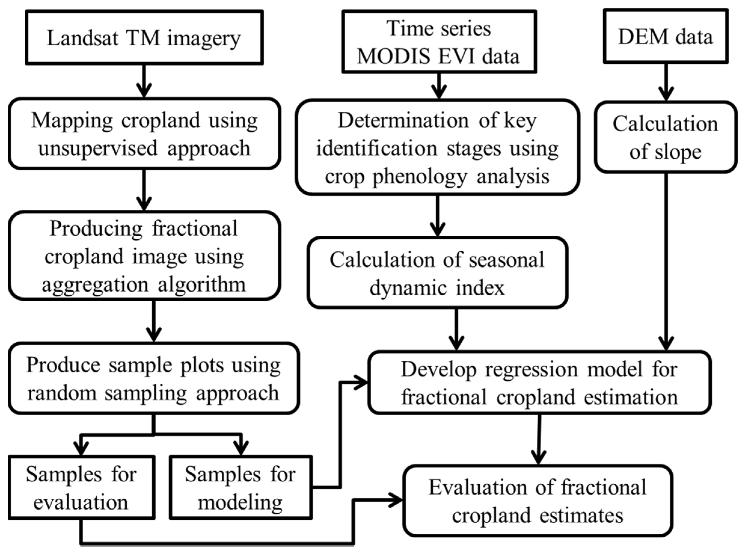
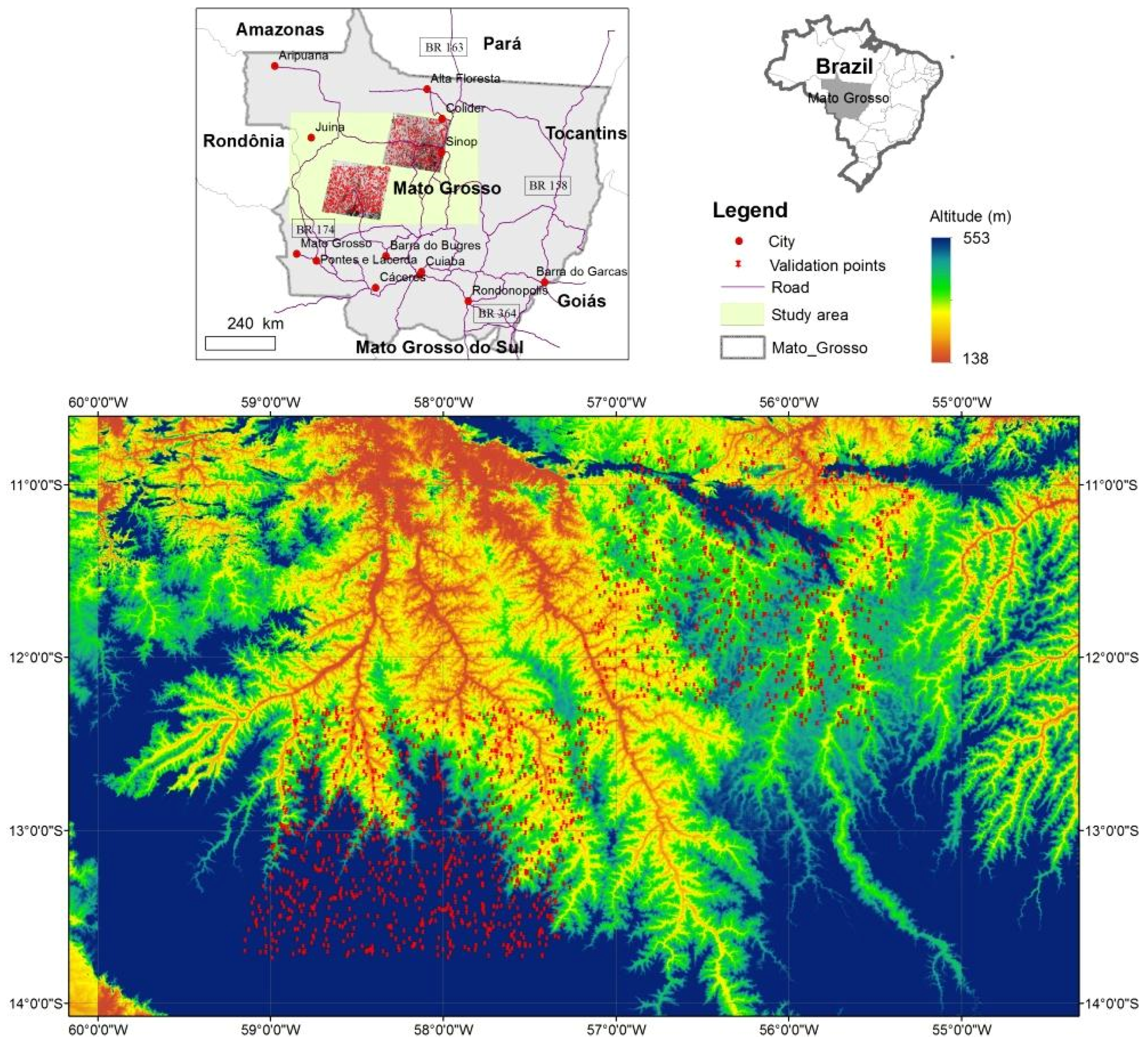
2. Study Area and Materials

The study area is located in the central and western part of Mato Grosso State, Brazil (Figure 1), featured by a transition from savanna in the south to tropical rainforests in the north. Soy is the main crop in this area and the sowing calendar for soybeans goes from mid-September to late December, depending on agricultural zoning for different soils, regions, and the onset of the rainy season [6,24]. According to IBGE 2015 (The Brazilian Institute of Geography and Statistics), area planted in soybeans increased by 5.59 million ha from 1995 (2.34 million ha) to 2013 (7.93 million ha). In Mato Grosso State, six cropping types (soy–corn, soy–cotton, soy–millet, soy–soy, cotton and pasture) account for 91.5% of reported agricultural land area [24]. These planting structures include single and double cropping systems.

Figure 1. Study area—part of Mato Grosso State, Brazil.

Figure 1. Study area—part of Mato Grosso State, Brazil.

In this research, two Landsat Thematic Mapper (TM) images acquired in 2011 (path/row: 228/69 and 227/68) were downloaded from United States Geological Survey (USGS) [38]. An unsupervised classification (i.e., ISODATA) was used to classify the Landsat multispectral bands (six spectral bands) with 30 m spatial resolution into 50 clusters. An analyst assigned each cluster into cropland or others through visual interpretation of the TM color composites and QuickBird images. The cropland distribution was examined visually to make sure no obvious misclassification occurred. Using the mean algorithm the cropland imagery with 30 m spatial resolution was aggregated into a new image with a cell size of 250 m for generating fractional cropland data in order to match the cell size of MODIS EVI data. The data were reprojected from its original Universal Transverse Mercator (UTM) coordinate system to Lambert Azimuthal Equal Area Projection.

Time series MODIS EVI product (MOD13Q1, h12v10) from July 2001 to July 2011 were downloaded from the USGS GLOVIS website as well. The originally sinusoidal projection was converted to the Lambert Azimuthal Equal Area Projection. SRTM (Shuttle Radar Topography Mission) DEM (digital elevation model) data with 90 m spatial resolution were downloaded from USGS [39].

3. Methods

Figure 2 illustrates the framework of mapping fractional cropland distribution using the MODIS EVI data and the two Landsat TM images. The major steps include: (1) extract cropland from Landsat TM imagery using unsupervised classification, aggregate the cropland image from 30 m cell size to 250 m cell size for producing fractional cropland distribution using the mean algorithm, and select sample plots using random sampling technique. Half of the selected samples were used for development of regression model and the other half were used to evaluate the estimates; (2) identify three key stages—sowing, growing, and harvest using the crop phenology analysis of time series MODIS EVI data and then calculate SDI; (3) develop a regression model for estimating fractional cropland by relating SDI and TM-derived fraction cropland data; and (4) evaluate the fractional cropland estimates using the SDI-based approach. The first step—extraction of cropland reference data from Landsat imagery was briefly described in Section 2. The following subsections describe the remaining steps.

Figure 2. Framework of fractional cropland mapping approach using the integration of time series MODIS (Moderate-resolution Imaging Spectroradiometer) Enhanced Vegetation Index (EVI) and Landsat Thematic Mapper (TM) data.

Figure 2. Framework of fractional cropland mapping approach using the integration of time series MODIS (Moderate-resolution Imaging Spectroradiometer) Enhanced Vegetation Index (EVI) and Landsat Thematic Mapper (TM) data.

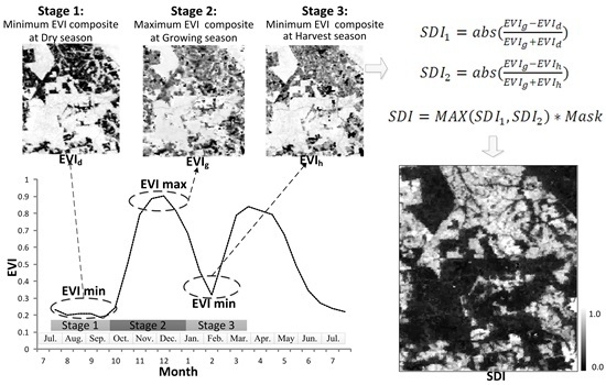
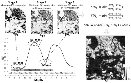
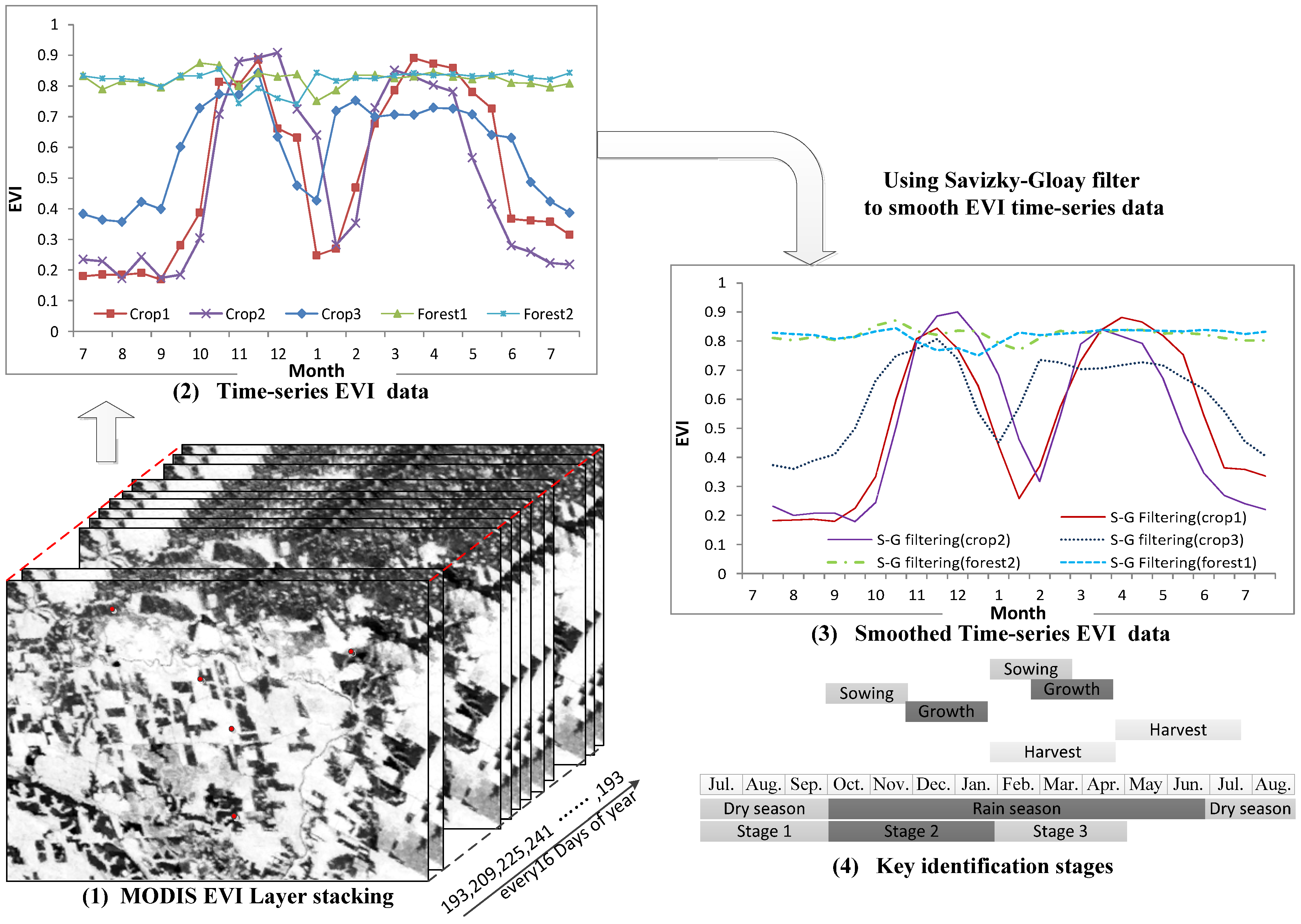
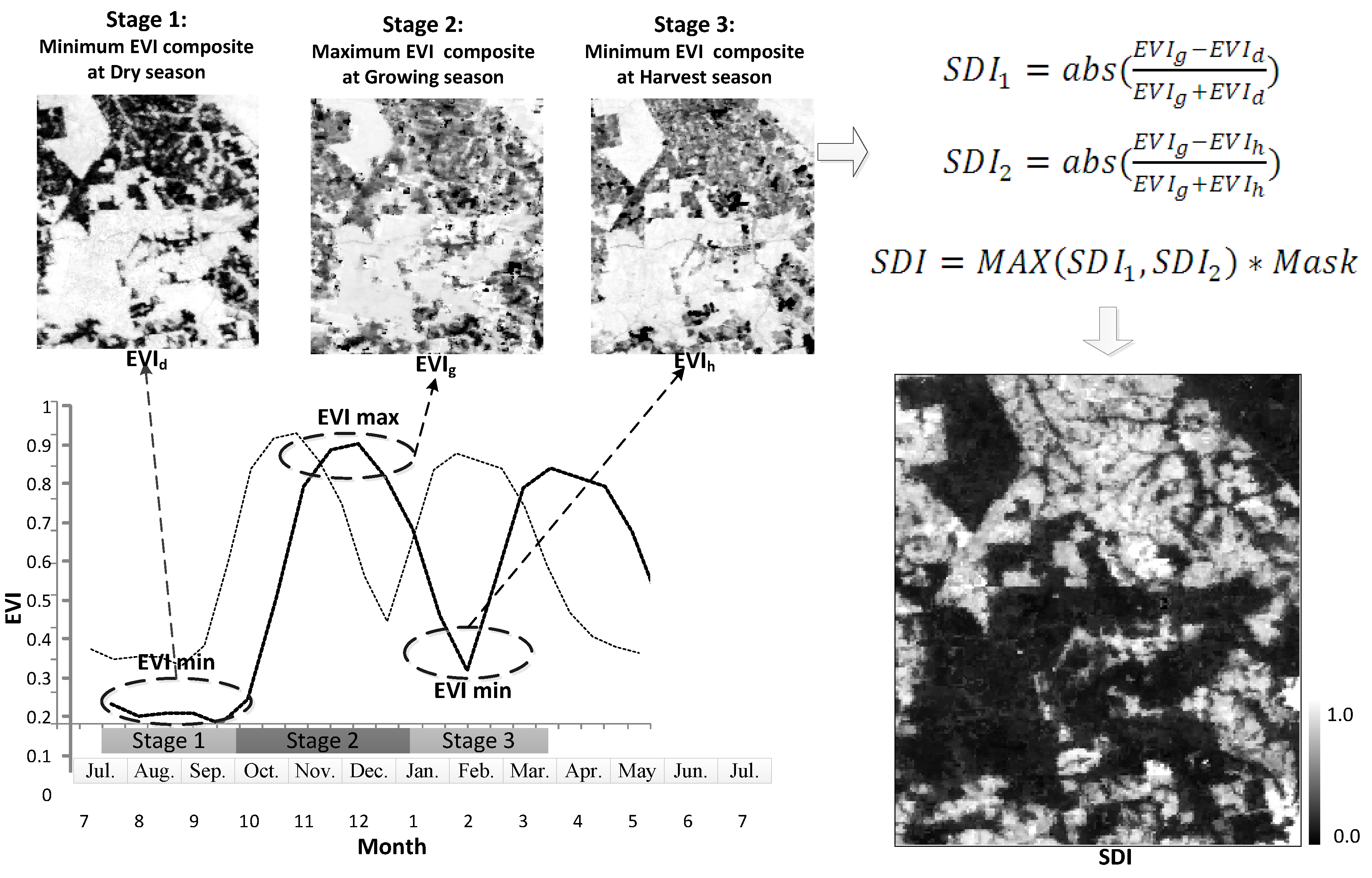
3.1. EVI Profiles and Crop Phenology Analysis

The seasonal patterns of croplands provide the foundation for cropland extraction using time series remote sensing imagery. Crop phenology is primary information for cropland mapping based on the spectral-temporal crop growth profile analysis. Crops have their own characteristics in the stages of planting, growing and maturing compared to other vegetation types such as forests. In Figure 3 we illustrate the EVI time series profiles for different land cover types based on the cropping system in Mato Grosso State. Through a year the EVI values in croplands vary drastically in different stages from sowing and growing to harvest. In contrast, forest has constant EVI profiles throughout the year. Crop phenology analysis is used to determine the key identification stages (KIS): sowing (Stage 1—from dry to wet season transition), growing (Stage 2), and harvest (Stage 3) seasons. Figure 3 implies that croplands can be identified from the three stages, instead of time series data of an entire year. This is critical for mapping cropland distribution in tropical and subtropical regions because of the cloud cover problem resulting in the difficulty in acquisition of cloud-free imagery.

Figure 3. Determination of key identification stages based on crop phenology analysis.

Figure 3. Determination of key identification stages based on crop phenology analysis.

3.2. Time Sparse Resampling (TSR)

Cloud contamination and noise are still common in the MODIS vegetation index composites. The Savitzky–Golay (S-G) filter is often used to reduce this problem [40,41,42,43]. Based on the regional crop phenology, a time sparse resampling (TSR) algorithm was proposed at the basis of the S-G filter (See Figure 4). The TSR algorithm was used to produce a cloud-free composite at different crop growth stages and to reduce the effect of the large variation of EVI profiles within each season. The time series EVI profile contains a large variation in croplands within a single year. The TSR used several images from the time series to produce a stable indicative factor within each season. For example, in Mato Grosso, Brazil, the croplands in the sowing season (from September to October) have very limited vegetation cover, a minimum EVI value is used in this period. The crops in growing season (November, December, and January) have the highest biomass, thus a maximum EVI value is selected. In the first harvest season (from January to March), there is a valley in annual crop growth profile, thus, the TSR algorithm is adjusted to acquire the minimum EVI value in the harvest season. The TSR is used to generate a new EVI composite in KIS as expressed in Equations (1)–(3).

$${\text{EVI}}_{\text{d}}=\text{MIN}({\text{EVI}}_{225},{\text{EVI}}_{241},{\text{EVI}}_{257},{\text{EVI}}_{273},{\text{EVI}}_{289})$$

(1)

$${\text{EVI}}_{\text{g}}=\text{MAX}({\text{EVI}}_{305},{\text{EVI}}_{321},{\text{EVI}}_{337},{\text{EVI}}_{353},{\text{EVI}}_{001}),$$

(2)

$${\text{EVI}}_{\text{h}}=\text{MIN}({\text{EVI}}_{017},{\text{EVI}}_{033},{\text{EVI}}_{049},{\text{EVI}}_{065},{\text{EVI}}_{081}),$$

(3)

where ${\text{EVI}}_{017},{\text{EVI}}_{033}$,……, ${\text{EVI}}_{353}$ are the multi-temporal 16-day composite L3 MODIS EVI products (MOD13Q1, 250 m spatial resolution) acquired in a year and the number subscript is the day of the year (DOY). ${\text{EVI}}_{\text{d}}$, EVI_g, and EVI_h are cloud-free EVI composites from the dry to wet transition, growth, and harvest seasons.

Figure 4. The Enhanced Vegetation Index (EVI) features at different crop growth stages and the seasonal dynamic index.

Figure 4. The Enhanced Vegetation Index (EVI) features at different crop growth stages and the seasonal dynamic index.

3.3. Seasonal Dynamic Index (SDI)

According to the EVI fluctuations at the different crop stages, the variation of EVI in a pixel can be assumed to have a positive correlation with the proportion of cropland area. Based on this hypothesis, the seasonal dynamic index (SDI) model is proposed through the EVI composites at different stages, as shown in Figure 4 for a typical crop phenology curve. Thus, SDI can be expressed as follows:

$$\text{SDI}=\text{MAX}\left({\text{SDI}}_1,{\text{SDI}}_2\right)\times \text{Mask}$$

(4)

$${\text{SDI}}_1=\text{abs}(\frac{{\text{EVI}}_{\text{g}}-{\text{EVI}}_{\text{d}}}{{\text{EVI}}_{\text{g}}+{\text{EVI}}_{\text{d}}})$$

(5)

$${\text{SDI}}_2=\text{abs}(\frac{{\text{EVI}}_{\text{g}}-{\text{EVI}}_{\text{h}}}{{\text{EVI}}_{\text{g}}+{\text{EVI}}_{\text{h}}})$$

(6)

$$\text{Mask}={\text{Pas}}_{\text{mask}}\times {\text{Slp}}_{\text{mask}}$$

(7)

where $\text{SDI}$ is seasonal dynamic index and ${\text{SDI}}_1$ and ${\text{SDI}}_2$ correspond to the seasonal dynamic index at different crop cycles. Considering the positive values of ${\text{SDI}}_1$ and ${\text{SDI}}_2$ in the double cropping system and negative values in the single cropping system, abs (absolute value) is used. To be classified as cropland, in addition to slope restrains, the pixel should meet three conditions (see Figure 4): EVI has (1) low value in the sowing period (Stage 1); (2) high value in the growing period (Stage 2); and (3) low value in the harvest period (Stage 3). In order to improve fractional cropland estimation accuracy, Mask is used as an indicator for calculating cropland fraction, which includes terrain (slope) mask and grassland (or savanna) mask. Here the slope mask and grassland mask are defined as follows:

(1)

${\text{Slp}}_{\text{mask}}$ is the topographic factor mask which the slope is derived from SRTM data. A threshold of 12% is used for ${\text{Slp}}_{\text{mask}}$, that is, the pixels having slopes greater than 12% are excluded from calculation, because a relatively flat landscape is required for allowing the use of farm machinery [21]. Therefore, ${\text{Slp}}_{\text{mask}}$ is assigned to 1 when slope is less than 12%; otherwise, ${\text{Slp}}_{\text{mask}}$ is assigned to 0.

(2)

${\text{Pas}}_{\text{mask}}$ is a pasture mask. For ${\text{Pas}}_{\text{mask}}$, the ratio of ${\text{SDI}}_1$ and ${\text{SDI}}_2$ is used to discriminate grassland and cropland. ${\text{SDI}}_1$ and ${\text{SDI}}_2$ have high value in double cropping, but ${\text{SDI}}_1$ has low value and ${\text{SDI}}_2$ has high value in single cropping. In contrast, grass land has a high value in ${\text{SDI}}_1$ and a low value in ${\text{SDI}}_2$. Based on trial and error testing a threshold of 2.5 is used. That is, if the ratio of ${\text{SDI}}_1$ and ${\text{SDI}}_2$ is greater than 2.5, the pixel is assigned to 0; otherwise, the pixel is assigned to 1.

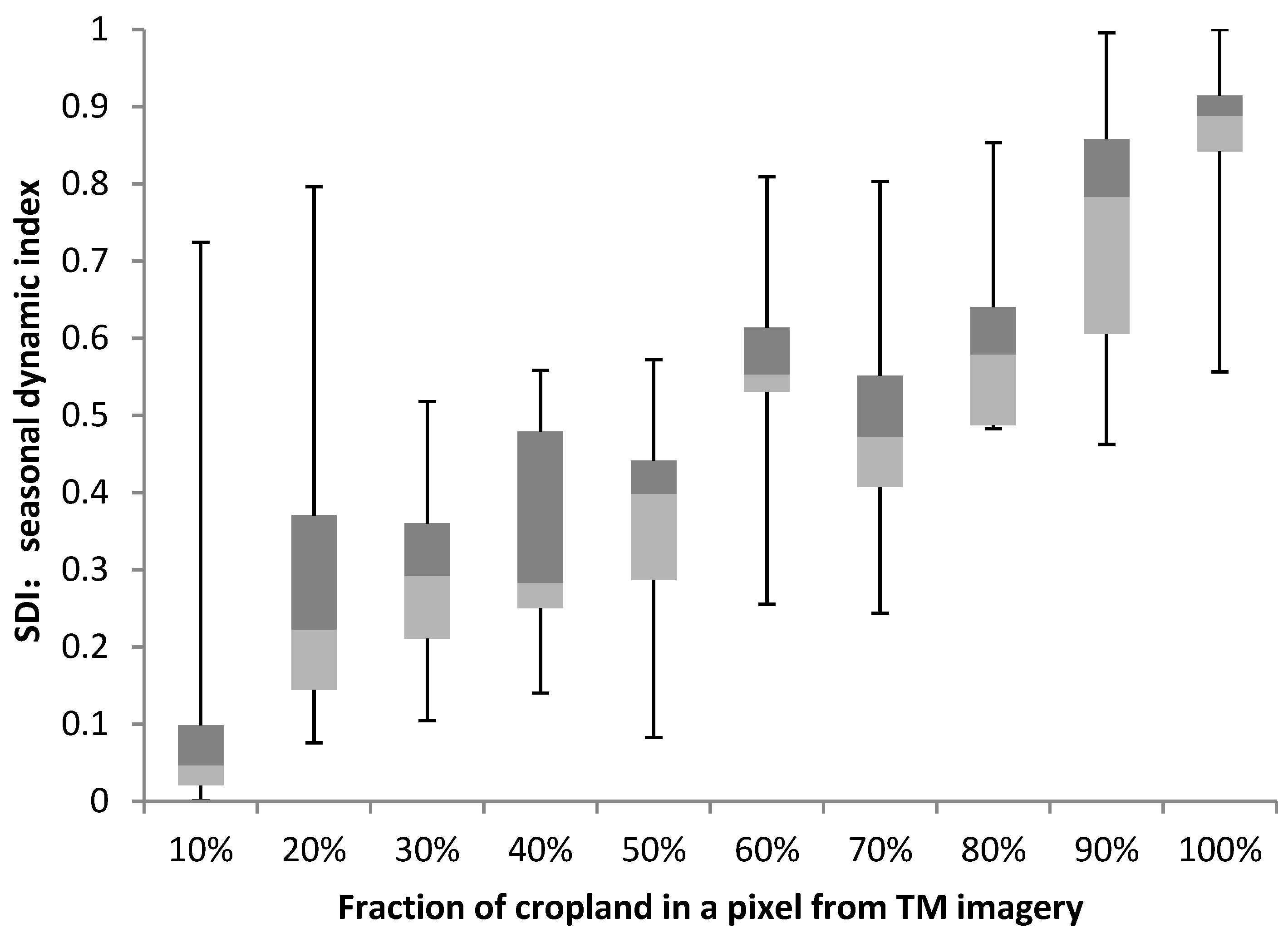
3.4. Analysis of the Relationship between SDI and Fraction Croplands

The Landsat-derived cropland imagery was aggregated to generate fractional cropland imagery with the same cell size as the SDI imagery. A total of 1000 sample plots were randomly selected from the overlapping regions between the fractional cropland imagery and the SDI imagery to extract the fraction value and corresponding SDI value at the same locations. The box whisker plot approach was used to examine SDI features, representing the graphical distribution of fractional cropland in a sample plot against the pixel SDI value (Figure 5). The fractional values ranging from 0% to 100% were separated into 10 groups with an interval of 10%. The SDI values range from 0 to 1 depending on the proportion of cropland cover in a MODIS pixel. In general, higher proportions of cropland in a sample plot correspond to a higher SDI values, as shown in Figure 5. This implies that the fraction of cropland in sample plots has a linear relationship with SDI values. This provides the foundation for developing a linear regression model for estimating fractional cropland values using the SDI variable.

Figure 5. The relationship between seasonal dynamic index (SDI) and fractional croplands.

Figure 5. The relationship between seasonal dynamic index (SDI) and fractional croplands.

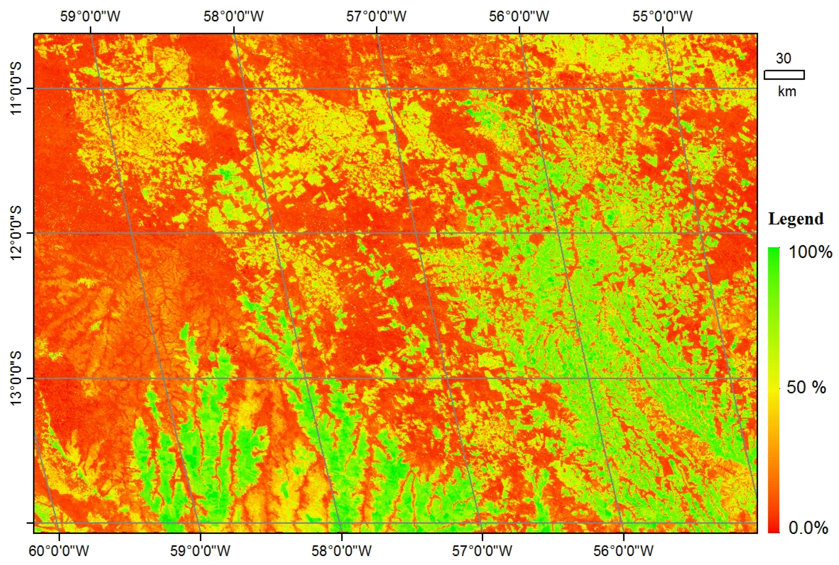
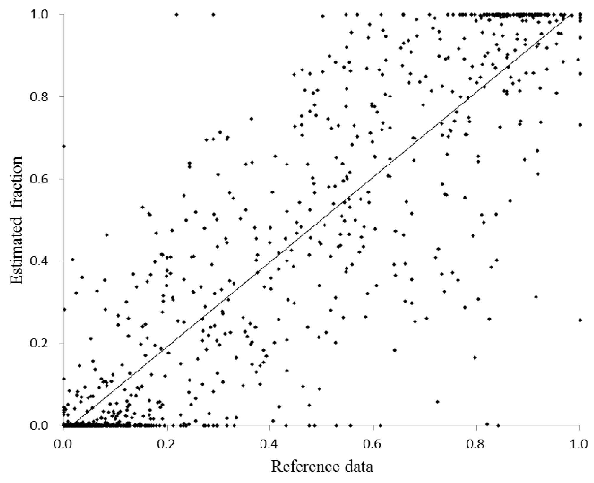
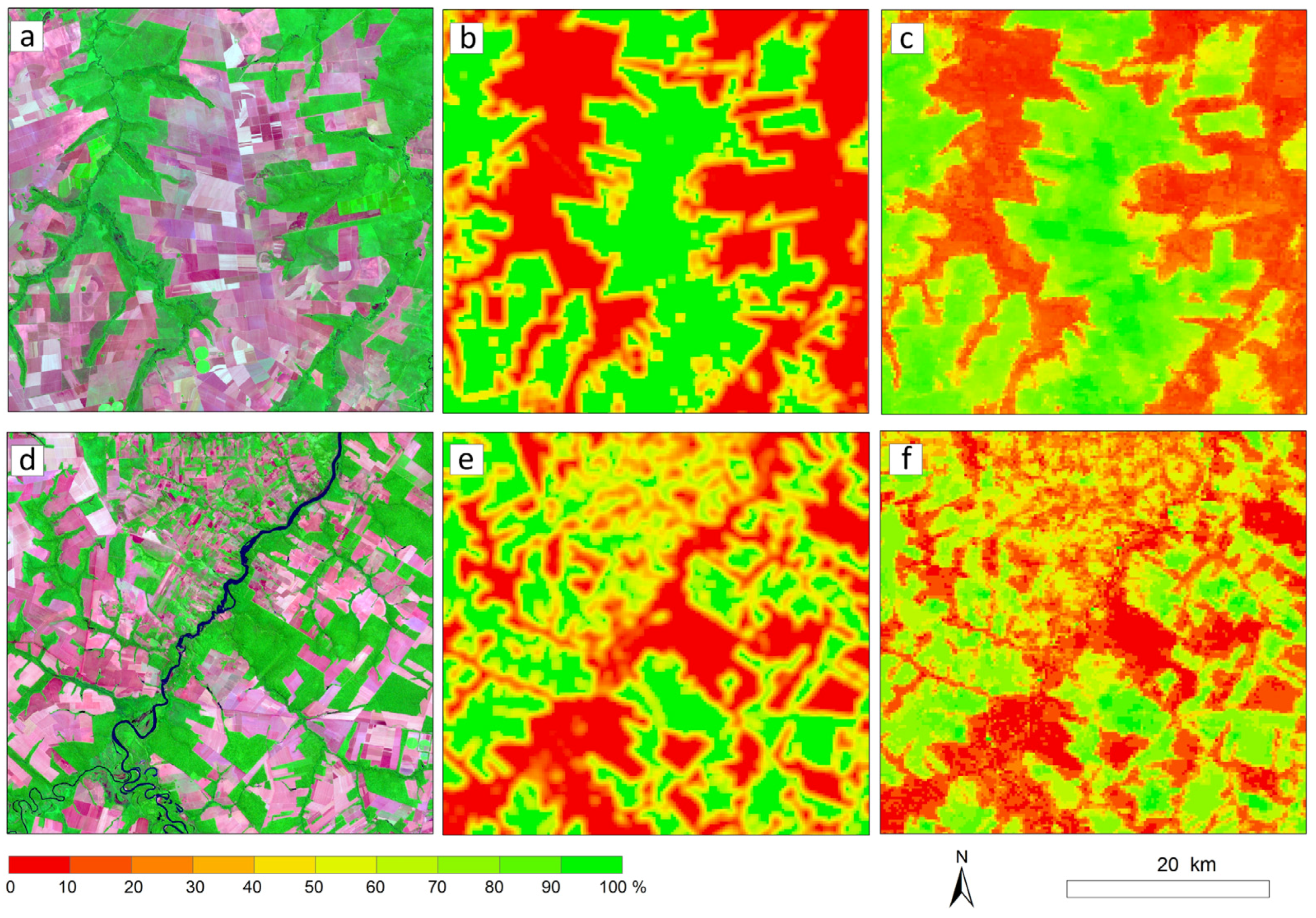
3.5. Mapping of Fractional Cropland Distribution and Evaluation of the Estimates

Based on the randomly selected 500 test samples, a regression model was developed to estimate fractional cropland areas for the whole study area, in which the fractional cropland data from TM data were used as a dependent variable, and SDI was used as an independent variable. The coefficient of determination (R²) was used to evaluate the fitness of the regression model because it measures the percentage of variation explained by the regression model.

Since the cropland estimation for each pixel is a fraction value, the traditional pixel-based classification assessment approach [43,44] cannot be directly used for the evaluation of this estimates. Therefore, root-mean squared error (RMSE) and the scatterplot between reference data and estimates were used to evaluate the fractional cropland estimation results.

3.6. Application of the Proposed Approach to Other Dates for Mapping Fractional Cropland Distribution

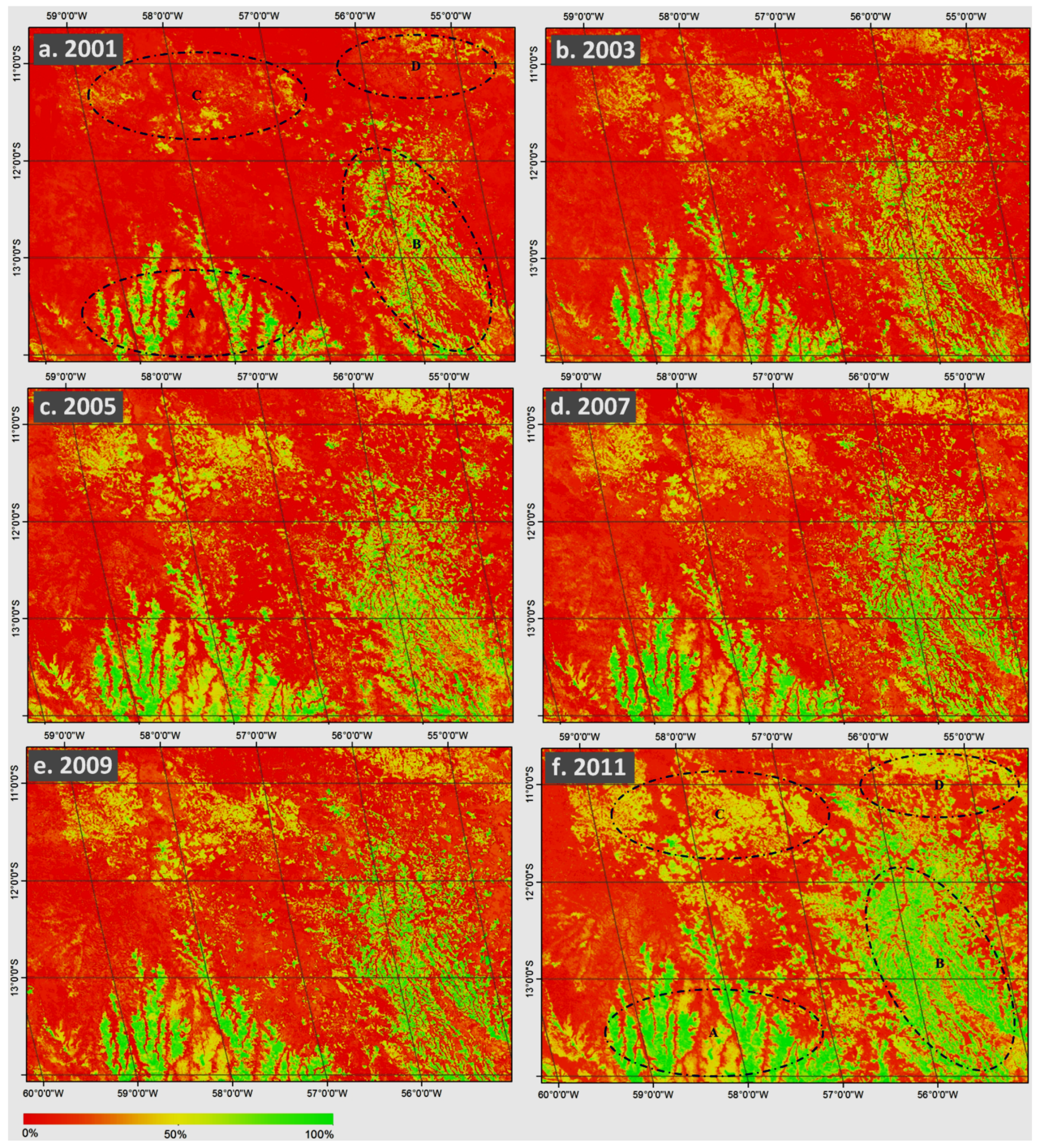
The above-mentioned approach is based on the 2011 MODIS EVI data and two Landsat TM images in Mato Grosso. In order to explore the transferability of this proposed approach, we applied this approach to other years of MODIS EVI data in the same study area for estimating fractional cropland distribution. The time series EVI images from 2001 to 2011 at two-year intervals were collected. The SDI image for each selected year was developed using the methods discussed above. The same regression model which was developed from the relationship between the 2011 SDI and corresponding fractional cropland data from Landsat TM imagery was then applied to each SDI image. The spatial patterns of the fractional cropland distribution were visually compared, especially for four typical sites within the study area.

4. Results

A regression model, that is, f_crop =1.1959 × SDI − 0.03, was developed and it was used to map fractional cropland distribution for entire study area (see Figure 6). In this factional map, the croplands are concentrated in southern and eastern parts with high fraction values, but are scattered in northern and western parts with fractional values of less than 50% in a pixel.

Figure 6. Fractional cropland distribution which is developed using the regression model based on MODIS EVI data in Mato Grosso, Brazil.

Figure 6. Fractional cropland distribution which is developed using the regression model based on MODIS EVI data in Mato Grosso, Brazil.

In order to examine the impacts of different cropland patch sizes on fractional cropland mapping performance, Figure 7 provides a comparison of cropland distributions between two sites: Site 1 (Figure 7a–c) representing large patch sizes of croplands, and site 2 (Figure 7d–f) representing the complex land cover composition with relatively small patch sizes of croplands. The results indicate that the cropland estimates with large patch sizes have similar spatial patterns with the cropland distributions from Landsat data (Figure 7a–c), but the croplands with relatively small patch sizes have different spatial patterns (Figure 7d–f) because the complex composition of different land covers in a pixel results in relatively poor estimates. This implies that the complex landscape of the study area may be a major factor resulting in poor performance of cropland estimation.

Figure 7. A comparison of fractional cropland distributions between Landsat-derived reference data and the SDI-based estimates (note: (a–c) represent Landsat TM color composite (7/4/2 bands), fractional cropland distribution from Landsat imagery, and fractional cropland distribution from MODIS EVI data at typical site 1, respectively; (d–f) represent Landsat TM 7/4/2 band color composite, fractional cropland distribution from Landsat imagery, and fractional cropland distribution from MODIS EVI data at typical site 2, respectively).

Figure 7. A comparison of fractional cropland distributions between Landsat-derived reference data and the SDI-based estimates (note: (a–c) represent Landsat TM color composite (7/4/2 bands), fractional cropland distribution from Landsat imagery, and fractional cropland distribution from MODIS EVI data at typical site 1, respectively; (d–f) represent Landsat TM 7/4/2 band color composite, fractional cropland distribution from Landsat imagery, and fractional cropland distribution from MODIS EVI data at typical site 2, respectively).

The scatterplot between the estimates and reference data based on the 2011 test samples are illustrated in Figure 8. A RMSE of 0.14 and the correlation coefficient of 0.89 were obtained, indicating a good overall estimation performance. The major errors are from two aspects, the pixels having fraction values of less than 0.2 or more than 0.8. This implies that the SDI-based model cannot accurately estimate the fraction values when the cropland proportion is greater than 80% or smaller than 20% in a MODIS pixel.

Figure 8. The relationship between estimates from SDI and corresponding cropland fraction reference data from Landsat TM data in 2011.

Figure 8. The relationship between estimates from SDI and corresponding cropland fraction reference data from Landsat TM data in 2011.

The SDI-based approach was used to estimate fractional cropland distribution between 2001 and 2009 in two-year intervals, which the regression model was developed from the 2011 datasets. A comparison of the fractional cropland distributions among these years (Figure 9) indicates the rapid cropland expansion in the study area. As shown in the sites a, b, c, and d in Figure 9, major cropland distribution and expansion is located in southern and southeastern parts of the study area. This Figure also implies the feasibility of transferring the same model to different dates.

Figure 9. A comparison of the developed fractional cropland distributions between 2001 and 2011 at a two-year interval, which is developed using the SDI-based approach (a–f represent the fractional cropland distribution in 2001–2011).

Figure 9. A comparison of the developed fractional cropland distributions between 2001 and 2011 at a two-year interval, which is developed using the SDI-based approach (a–f represent the fractional cropland distribution in 2001–2011).

5. Discussion

Continuous time series NDVI or EVI data can provide detailed vegetation phenology information, thus they are often used for mapping cropland distribution [14,20,21,28]. However, in tropical and subtropical regions, it is impossible to collect continuous time series optical sensor data (e.g., MODIS) due to the cloud cover problem. Therefore, we proposed the TSR algorithm in this research to solve the data collection problem. The TSR can enhance the differences between cropland and other land cover types, and so aid in the separation of cropland from other land cover. Meanwhile, the use of SDI can help explore the impacts of single or double cropping systems on cropland mapping. The linear relationship between SDI and fractional cropland values in a pixel further documents the potential to estimate fractional cropland in a large area using the SDI image.

This research indicated that errors occurred more frequently when the proportion of croplands in a pixel is very high or very low. When pixels have high proportion of croplands such as greater than 0.8, SDI is often saturated; however, when the pixels have low proportion of croplands such as less than 0.2, SDI is not sensitive enough, resulting in underestimation of cropland area. This situation is similar to previous studies when the cell size of the remotely sensed data is larger than the size of individual objects, this is especially true in urban landscapes, and referred to as mixed pixels [45]. The results illustrated in Figure 8 also confirm that the small patch size of croplands, i.e., mixed pixels, is an important source of cropland mapping uncertainty.

Many previous “hard” classification methods such as thresholding approaches or classification algorithms are used to map cropland distribution [6,20,21,27], but the mixed pixel problem inherent in the coarse spatial resolution imagery (e.g., MODIS) often results in large uncertainty in cropland area statistics, resulting in poor area estimation and inaccurate spatial patterns. Although spectral mixture analysis presents an effective way to decompose the spectral reflectance of a pixel into different proportions, and has proven valuable in medium spatial resolution images such as Landsat or hyperspectral data [12,46,47], this approach is not so promising in coarse spatial resolution images such as MODIS due to the complex land cover composition and the difficulty in identifying suitable endmembers in large areas. This research using Landsat-derived cropland data as reference to establish a regression model by relating it to the SDI variable has proven feasible in estimating fractional cropland.

In addition to the spectral mixture analysis in reducing the mixed pixel problem, another approach is the use of data fusion of multi-resolution/sensor data [48,49,50,51]. However, in a large area, the data fusion of Landsat TM and MODIS data may not be cost effective or may be not necessary because Landsat TM image can reliably provide cropland classification. In addition, in tropical regions like this study area, Landsat images are not available for many sites due to the cloud cover problem, thus this kind data fusion is not feasible. Therefore, this research proposed the combination of MODIS and a limited number of Landsat TM image to solve this data availability problem. A similar work has been used for mapping fractional forest distribution [45]. A combination of multi-source data such as MODIS, Landsat images, and ancillary data is an alternative to improve cropland mapping performance [25]. However, attention should be paid to potential geometric errors between different data sources. For example, the misregistration between Landsat and MODIS can reach a minimum of 50 m (nadir) [52].

The application of using this approach to other years of MODIS data in the same study area has indicated its value in rapidly mapping fractional cropland distribution in a large area. However, caution should be taken when attempting to transfer this approach to other study areas due to the different land cover composition. For future study, subpixel based approaches using nonparametric algorithms may be another direction for better extracting croplands, especially when accurate cropland area statistics are required [6,31,35].

6. Conclusions

The proposed SDI-based approach provided a feasible way for mapping fractional cropland distribution in Mato Grosso, Brazil. In summary, the following conclusions can be obtained:

(1)

The use of the TSR algorithm based on crop phenology analysis effectively solved the difficulty in collecting continuous time series data because of cloud contamination and noise.

(2)

The proposed SDI approach effectively extracted fractional cropland distribution in a large area.

(3)

The use of masks based on slope and pasture further reduced the confusion between croplands and pastures, and thus improved cropland mapping performance.

(4)

A RMSE of 0.14 was obtained for the cropland distribution in 2011.

References

1. Ramankutty, N.; Evan, A.T.; Monfreda, C.; Foley, J.A. Farming the planet: 1. Geographic distribution of global agricultural lands in the year 2000. Glob. Biogeochem. Cycles 2008, 22. [Google Scholar] [CrossRef]
2. Godfray, H.C.J.; Beddington, J.R.; Crute, I.R.; Haddad, L.; Lawrence, D.; Muir, J.F.; Pretty, J.; Robinson, S.; Thomas, S.M.; Toulmin, C. Food security: The challenge of feeding 9 billion people. Science 2010, 327, 812–818. [Google Scholar] [CrossRef] [PubMed]
3. Tilman, D.; Balzer, C.; Hill, J.; Befort, B.L. Global food demand and the sustainable intensification of agriculture. Proc. Natl. Acad. Sci. USA 2011, 108, 20260–20264. [Google Scholar] [CrossRef] [PubMed]
4. Fritz, S.; See, L.; You, L.; Justice, C.; Becker-Reshef, I.; Bydekerke, L.; Cumani, R.; Defourny, P.; Erb, K.; Foley, J. The need for improved maps of global cropland. Eos Trans. Am. Geophys. Union 2013, 94, 31–32. [Google Scholar] [CrossRef]
5. Pittman, K.; Hansen, M.C.; Becker-Reshef, I.; Potapov, P.V.; Justice, C.O. Estimating global cropland extent with multi-year MODIS data. Remote Sens. 2010, 2, 1844–1863. [Google Scholar] [CrossRef]
6. Arvor, D.; Jonathan, M.; Meirelles, M.S.P.; Dubreuil, V.; Durieux, L. Classification of MODIS EVI time series for crop mapping in the state of Mato Grosso, Brazil. Int. J. Remote Sens. 2011, 32, 7847–7871. [Google Scholar] [CrossRef]
7. Thenkabail, P.; Lyon, J.G.; Turral, H.; Biradar, C. Remote Sensing of Global Croplands for Food Security; CRC Press: Baco Raton, FL, USA, 2009. [Google Scholar]
8. Thenkabail, P.S.; Biradar, C.M.; Noojipady, P.; Dheeravath, V.; Li, Y.; Velpuri, M.; Gumma, M.; Gangalakunta, O.R.P.; Turral, H.; Cai, X. Global irrigated area map (giam), derived from remote sensing, for the end of the last millennium. Int. J. Remote Sens. 2009, 30, 3679–3733. [Google Scholar] [CrossRef]
9. Thenkabail, P.S.; Hanjra, M.A.; Dheeravath, V.; Gumma, M. A holistic view of global croplands and their water use for ensuring global food security in the 21st century through advanced remote sensing and non-remote sensing approaches. Remote Sens. 2010, 2, 211–261. [Google Scholar] [CrossRef] [Green Version]
10. Wulder, M.A.; Masek, J.G.; Cohen, W.B.; Loveland, T.R.; Woodcock, C.E. Opening the archive: How free data has enabled the science and monitoring promise of Landsat. Remote Sens. Environ. 2012, 122, 2–10. [Google Scholar] [CrossRef]
11. Lu, D.; Li, G.; Moran, E.; Hetrick, S. Spatiotemporal analysis of land-use and land-cover change in the Brazilian Amazon. Int. J. Remote Sens. 2013, 34, 5953–5978. [Google Scholar] [CrossRef] [PubMed]
12. Lu, D.; Li, G.; Moran, E. Current situation and needs of change detection techniques. Int. J. Image Data Fusion 2014, 5, 13–38. [Google Scholar] [CrossRef]
13. Asner, G.P. Cloud cover in Landsat observation of the Brazilian Amazon. Int. J. Remote Sens. 2001, 22, 3855–3862. [Google Scholar] [CrossRef]
14. Wardlow, B.D.; Egbert, S.L. Large-area crop mapping using time-series MODIS 250 m NDVI data: An assessment for the U.S. Central great plains. Remote Sens. Environ. 2008, 112, 1096–1116. [Google Scholar] [CrossRef]
15. Moulin, S.; Kergoat, L.; Viovy, N.; Dedieu, G. Global-scale assessment of vegetation phenology using NOAA/AVHRR satellite measurements. J. Clim. 1997, 10, 1154–1170. [Google Scholar] [CrossRef]
16. Braswell, B.H.; Hagen, S.C.; Frolking, S.E.; Salas, W.A. A multivariable approach for mapping sub-pixel land cover distributions using misr and MODIS: Application in the Brazilian Amazon region. Remote Sens. Environ. 2003, 87, 243–256. [Google Scholar] [CrossRef]
17. Morton, D.C.; DeFries, R.S.; Shimabukuro, Y.E.; Anderson, L.O.; Arai, E.; del Bon Espirito-Santo, F.; Freitas, R.; Morisette, J. Cropland expansion changes deforestation dynamics in the southern Brazilian amazon. Proc. Natl. Acad. Sci. USA 2006, 103, 14637–14641. [Google Scholar] [CrossRef] [PubMed]
18. Arvor, D.; Meirelles, M.; Dubreuil, V.; Bégué, A.; Shimabukuro, Y.E. Analyzing the agricultural transition in Mato Grosso, Brazil, using satellite-derived indices. Appl. Geogr. 2012, 32, 702–713. [Google Scholar] [CrossRef]
19. Arvor, D.; Dubreuil, V.; Simões, M.; Bégué, A. Mapping and spatial analysis of the soybean agricultural frontier in Mato Grosso, Brazil, using remote sensing data. GeoJournal 2012, 78, 833–850. [Google Scholar] [CrossRef]
20. Victoria, D.D.C.; Paz, A.R.D.; Coutinho, A.C.; Brown, J.C. Cropland area estimates using MODIS-NDVI times series in the state of Mato Grosso, Brazil. Pesqui. Agropecu. Bras. 2012, 47, 1270–1278. [Google Scholar] [CrossRef]
21. Brown, J.C.; Kastens, J.H.; Coutinho, A.C.; Victoria, D.D.C.; Bishop, C.R. Classifying multiyear agricultural land use data from Mato Grosso using time-series MODIS vegetation index data. Remote Sens. Environ. 2013, 130, 39–50. [Google Scholar] [CrossRef]
22. Zhang, M.; Wu, B.; Yu, M.; Zou, W.; Zheng, Y. Crop condition assessment with adjusted NDVI using the uncropped arable land ratio. Remote Sens. 2014, 6, 5774–5794. [Google Scholar] [CrossRef]
23. Shao, Y.; Lunetta, R.S.; Ediriwickrema, J.; Iiames, J. Mapping cropland and major crop types across the Great Lakes Basin using MODIS-NDVI data. Photogramm. Eng. Remote Sens. 2010, 76, 73–84. [Google Scholar] [CrossRef]
24. Gusso, A.; Arvor, D.; Ducati, J.R.; Veronez, M.R.; da Silveira, L.G., Jr. Assessing the MODIS crop detection algorithm for soybean crop area mapping and expansion in the Mato Grosso State, Brazil. Sci. World J. 2014, 2014, 863141. [Google Scholar] [CrossRef] [PubMed]
25. Thenkabail, P.S.; Wu, Z. An automated cropland classification algorithm (acca) for Tajikistan by combining Landsat, MODIS, and secondary data. Remote Sens. 2012, 4, 2890–2918. [Google Scholar] [CrossRef]
26. Lu, D.; Batistella, M.; Li, G.; Moran, E.; Hetrick, S.; Freitas, C.; Dutra, L.; Sant’Anna, S.J.S. Land use/cover classification in the Brazilian Amazon using satellite images. Braz. J. Agric. Res. 2012, 47, 1185–1208. [Google Scholar] [CrossRef] [PubMed]
27. Gusso, A.; Formaggio, A.R.; RizziII, R.; Adami, M.; Rudorff, B.F.T. Soybean crop area estimation by MODIS/EVI data. Remote Sens. 2012, 47, 425–435. [Google Scholar] [CrossRef]
28. Mingwei, Z.; Qingbo, Z.; Zhongxin, C.; Jia, L.; Yong, Z.; Chongfa, C. Crop discrimination in northern china with double cropping systems using fourier analysis of time-series MODIS data. Int. J. Appl. Earth Obs. Geoinf. 2008, 10, 476–485. [Google Scholar] [CrossRef]
29. Kehl, T.N.; Todt, V.; Veronez, M.R.; Cazella, S.C. Amazon rainforest deforestation daily detection tool using artificial neural networks and satellite images. Sustainability 2012, 4, 2566–2573. [Google Scholar] [CrossRef]
30. Zheng, B.; Myint, S.W.; Thenkabail, P.S.; Aggarwal, R.M. A support vector machine to identify irrigated crop types using time-series Landsat NDVI data. Int. J. Appl. Earth Obs. Geoinf. 2015, 34, 103–112. [Google Scholar] [CrossRef]
31. Lobell, D.B.; Asner, G.P. Cropland distributions from temporal unmixing of MODIS data. Remote Sens. Environ. 2004, 93, 412–422. [Google Scholar] [CrossRef]
32. Fisher, P. The pixel: A snare and a delusion. Int. J. Remote Sens. 1997, 18, 679–685. [Google Scholar] [CrossRef]
33. Defries, R.S.; Field, C.B.; Fung, I.; Justice, C.O.; Los, S.; Matson, P.A.; Matthews, E.; Mooney, H.A.; Potter, C.S.; Prentice, K.; et al. Mapping the land surface for global atmosphere biosphere models toward continuous distributions of vegetations functional properties. J. Geophys. Res. Atmos. 1995, 100, 20867–20882. [Google Scholar] [CrossRef]
34. Wu, J.; Shen, W.; Sun, W.; Tueller, P.T. Empirical patterns of the effects of changing scale on landscape metrics. Landsc. Ecol. 2002, 17, 761–782. [Google Scholar] [CrossRef]
35. Ozdogan, M. The spatial distribution of crop types from MODIS data: Temporal unmixing using independent component analysis. Remote Sens. Environ. 2010, 114, 1190–1204. [Google Scholar] [CrossRef]
36. Busetto, L.; Meroni, M.; Colombo, R. Combining medium and coarse spatial resolution satellite data to improve the estimation of sub-pixel NDVI time series. Remote Sens. Environ. 2008, 112, 118–131. [Google Scholar] [CrossRef]
37. DeFries, R.S.; Hansen, M.C.; Townshend, J.R.G. Global continuous fields of vegetation characteristics: A linear mixture model applied to multiyear 8 km AVHRR data. Int. J. Remote Sens. 2000, 21, 1389–1414. [Google Scholar] [CrossRef]
38. USGS GLOVIS. Available online: http://glovis.usgs.gov/ (accessed on 9 December 2015).
39. USGS. Available online: https://lpdaac.usgs.gov/ (accessed on 9 December 2015).
40. Ma, M.; Veroustraete, F. Reconstructing pathfinder AVHRR and NDVI time-series data for the north-west of China. Adv. Sp. Res. 2006, 37, 835–840. [Google Scholar] [CrossRef]
41. Chen, J.; Jönsson, P.; Tamura, M.; Gua, Z.; Matsushita, B.; Eklundh, L. A simple method for reconstructing a high-quality NDVI time-series data set based on the Savitzky-Golay filter. Remote Sens. Environ. 2004, 91, 332–344. [Google Scholar] [CrossRef]
42. Savitzky, A.; Golay, M.J.E. Smoothing and differentiation of data by simplified least squares procedures. Anal. Chem. 1964, 36, 1627–1639. [Google Scholar] [CrossRef]
43. Congalton, R.G. A review of assessing the accuracy of classifications of remotely sensed data. Remote Sens. Environ. 1991, 37, 35–46. [Google Scholar] [CrossRef]
44. Congalton, R.G.; Green, K. Assessing the Accuracy of Remotely Sensed Data: Principles and Practices; CRC press: Baco Raton, FL, USA, 2008. [Google Scholar]
45. Lu, D.; Batistella, M.; Moran, E.; Hetrick, S.; Alves, D.; Brondizio, E. Fractional forest cover mapping in the Brazilian Amazon with a combination of MODIS and TM images. Int. J. Remote Sens. 2011, 32, 7131–7149. [Google Scholar] [CrossRef]
46. Adams, J.B.; Sabol, D.E.; Kapos, V.; Filho, R.A.; Roberts, D.A.; Smith, M.O.; Gillespie, A.R. Classification of multispectral images based on fractions of endmembers: Application to land cover change in the Brazilian Amazon. Remote Sens. Environ. 1995, 52, 137–154. [Google Scholar] [CrossRef]
47. Mustard, J.F.; Sunshine, J.M. Spectral analysis for earth science: Investigations using remote sensing data. Remote Sens. Earth Sci. Man. Remote Sens. 1999, 3, 251–307. [Google Scholar]
48. Zhang, J. Multisource remote sensing data fusion: Status and trends. Int. J. Image Data Fusion 2010, 1, 5–24. [Google Scholar] [CrossRef]
49. Gumma, M.K.; Thenkabail, P.S.; Hideto, F.; Nelson, A.; Dheeravath, V.; Busia, D.; Rala, A. Mapping Irrigated Areas of Ghana Using Fusion of 30 m and 250 m Resolution Remote-Sensing Data. Remote Sens. 2011, 3, 816–835. [Google Scholar] [CrossRef]
50. Ghamisi, P.; Benediktsson, J.A.; Phinn, S. Land-cover classification using both hyperspectral and LiDAR data. Int. J. Image Data Fusion 2015, 6, 189–215. [Google Scholar] [CrossRef]
51. Zhu, X.; Helmer, E.H.; Gao, F.; Liu, D.; Chen, J.; Lefsky, M.A. A flexible spatiotemporal method for fusing satellite images with different resolutions. Remote Sens. Environ. 2016, 172, 165–177. [Google Scholar] [CrossRef]
52. Wolfe, R.E.; Nishihama, M.; Fleig, A.J.; Kuyper, J.A.; Roy, D.P.; Storey, J.C.; Patt, F.S. Achieving sub-pixel geolocation accuracy in support of MODIS land science. Remote Sens. Environ. 2002, 83, 31–49. [Google Scholar] [CrossRef]