Modeling and Mapping Agroforestry Aboveground Biomass in the Brazilian Amazon Using Airborne Lidar Data

Abstract

Agroforestry has large potential for carbon (C) sequestration while providing many economical, social, and ecological benefits via its diversified products. Airborne lidar is considered as the most accurate technology for mapping aboveground biomass (AGB) over landscape levels. However, little research in the past has been done to study AGB of agroforestry systems using airborne lidar data. Focusing on an agroforestry system in the Brazilian Amazon, this study first predicted plot-level AGB using fixed-effects regression models that assumed the regression coefficients to be constants. The model prediction errors were then analyzed from the perspectives of tree DBH (diameter at breast height)—height relationships and plot-level wood density, which suggested the need for stratifying agroforestry fields to improve plot-level AGB modeling. We separated teak plantations from other agroforestry types and predicted AGB using mixed-effects models that can incorporate the variation of AGB-height relationship across agroforestry types. We found that, at the plot scale, mixed-effects models led to better model prediction performance (based on leave-one-out cross-validation) than the fixed-effects models, with the coefficient of determination (R²) increasing from 0.38 to 0.64. At the landscape level, the difference between AGB densities from the two types of models was ~10% on average and up to ~30% at the pixel level. This study suggested the importance of stratification based on tree AGB allometry and the utility of mixed-effects models in modeling and mapping AGB of agroforestry systems.

1. Introduction

Agroforestry denotes land use systems where woody perennials (trees, shrubs, palms, etc.) are cultivated on the same land units as agricultural crops and/or animals [1,2]. In this study, we use agroforestry as a general term to refer to the land use system of cultivating woody perennials, either polyculture or monoculture (i.e., plantation) on agricultural land, regardless the current existence of crops or animals. Over 10 million km² of agricultural lands have greater than 10% tree cover [3]. Through the provision of diversified products, agroforestry has been advocated and practiced by many countries to offer a wide range of economic, social, and ecological benefits: (1) increasing the per capita farm income by planning high-value tree products [4]; (2) improving soil fertility and land productivity [5]; (3) increasing household resilience [4]; (4) mitigating the impacts of climate variability and change [6,7]; (5) conserving biodiversity [8,9,10]; and (6) improving air and water quality [11,12,13].

Agroforestry offers high potential for carbon (C) sequestration [14] not only because the carbon density of agroforestry is usually higher than annual crops or pasture [15,16,17] but also because the trees produce fuelwood and timbers that otherwise would be harvested from natural forests [1]. The fine and coarse wood debris of plants are also stored in the soil C pool for long periods [18]. Thus, the role of agroforestry for C sequestration is increasingly recognized by the IPCC (Intergovernmental Panel on Climate Change) [19]. However, for agroforestry to be successful as a strategy for C sequestration, it is necessary to have sound detection and monitoring systems [20].

Remote sensing provides an effective way to estimate and monitor the biomass and C stock of different vegetation types [21] including agroforestry systems [22,23,24,25]. In particular, airborne lidar (Light Detection and Ranging) has emerged in the 21 century as the most accurate technology to quantify forest aboveground biomass (AGB) at the landscape level [21,26]. Lidar is especially powerful over forests of high biomass where passive optical imaging or radar sensors have saturation problems. One of the main advantages of lidar is that it can penetrate through the small canopy gaps for detecting vertical structure and extracting ground elevation. The height information derived from lidar is strongly related to biomass for most tree species. A large number of studies have reported the use of airborne lidar for mapping AGB in boreal (e.g., [27,28,29]), temperate (e.g., [30,31]), and tropical (e.g., [32,33,34,35,36]) forests.

Compared to the large body of literature of lidar remote sensing of carbon and biomass for forests, the use of this frontier technology for quantifying agroforestry AGB is very limited. One of the best examples of agroforestry of relative economic success of colonization in the Brazilian Amazon occurred in the Tomé-Açu [37]. Focusing on an agroforestry system in Tomé-Açu, this study aims to (1) predict plot-level agroforestry AGB using regular fixed-effects regression models that treat the regression coefficients as constants; (2) identify the causes of AGB prediction errors when such models are used; (3) propose new ways to stratify vegetation types and apply mixed-effects models to reduce the AGB prediction errors; and (4) discuss the challenges and future directions for modeling and mapping agroforestry AGB.

2. Study Area

This study was conducted in the Quatro Bocas district in the municipality of Tomé-Açu (2°28′S and 48°20′W), located in the northeastern region of Pará state in Brazil (Figure 1). The study area is 2 km by 5 km. Topography in the region is characterized by low flat plateaus, terraces, and lowlands with altitudes varying from 14 to 96 m. The soils are classified as Ferralsols, Plintosols, and Fluvisols. The average annual rainfall is 2300 mm [38]. The Tomé-Açu region has a humid mesothermal climate—Ami according to the Köppen classification—with high average annual temperatures (26 °C) and relative air humidity rate of about 85%. The original vegetation is lowland dense ombrophilous forest, which has been intensely altered. The landscape mosaic is dominated by pasture, agricultural fields, and secondary forests. Forest remnants are observed especially at the margins of streams.

Tomé-Açu started its agricultural development in the 1920’s, with the beginning of the Japanese immigration to the region. The immigrants implanted horticulture and, later, black pepper (Piper nigrum L.). They were provided with lands by the Brazilian government, which made technological development possible and turned Pará into the greatest black pepper producer in Brazil. With the decay of the black-pepper cycle from the 1970’s on, caused by fusarium blight, the farmers looked for new production alternatives. According to Homma [39], the way out of this ecological crisis for the immigrants was to diversify their activities, with emphasis in fruit crops, especially papaya, melon, acerola, orange, dende (oil palm), cupuacu, passion fruit, and other native and exotic fruit trees and vines that initiated a new economic cycle for the region. The current agroforestry systems (1 to 34 years old) have a great variety of fruit and timber tree species. Homma [40] pointed out that the success of the region’s agricultural development resulted from the Japanese-Brazilian farmers’ innovative thinking, their holistic view of future markets, and their social-minded spirit, which made possible the creation of the Cooperativa Agrícola Mista de Tomé-Açu (Camta) in 1931, whose intention was to sell vegetables and nowadays commercializes the agroforestry products (fruit, pulp, juice, and oil) in various countries.

Figure 1. The study area—Tomé-Açu at Pará state in Brazil (Data source: Lidar data were acquired in 2013 and 13 plots were measured in 2014) (Note: colors from red to blue represent the elevation of the laser points).

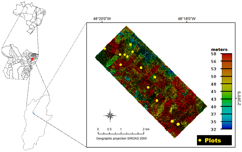
Figure 1. The study area—Tomé-Açu at Pará state in Brazil (Data source: Lidar data were acquired in 2013 and 13 plots were measured in 2014) (Note: colors from red to blue represent the elevation of the laser points).

3. Methods

3.1. Field Data Collection and AGB Estimation

Field inventory followed methods consistent with standardized protocols for tropical forests (e.g., [41]). Thirteen field plots of 30 m × 30 m were established in agroforestry regions using a differential GNSS (Trimble GeoXH-6000) during August and October 2014. The plot locations were selected to cover agroforestry fields with different ages and floristic compositions [22]. Diameter at breast height (DBH) was measured with metric tapes. Tree height was measured with tape and clinometer with the estimated accuracy of 10% of the tree height [42,43].

Over the 13 plots, the field crew collected measurements for a total of 1173 live trees to a minimum DBH of 5 cm from 22 species (Table 1). Four out of 13 plots grew monocultures including teak (plots 9 and 10), dende (plot 11), and cupuacu (plot 15), while the rest of the plots were mixed with two to eight species (Table 2).

Table 1. Tree species of the field plots and their wood densities.

Common Name	Scientific Name	Tree Count	ρ (g/cm3)	Type
Acai	Euterpe oleracea	287	0.41	Palm
Ameixa (Tallow plum)	Ximenia americana	108	0.64	Other
Andiroba	Carapa guianensis	7	0.57	Other
Cacau (Cocoa)	Theobroma glaucum	408	0.53	Other
Castanha dopara (Brazil nut)	Bertholletia excelsa	4	0.64	Other
Cupuacu	Theobroma grandiflorum	72	0.53	Other
Dende (American oil palm)	Elaeis oleifera	13	0.41	Palm
Embauba	Cecropia ficifolia	5	0.27	Other
Freijo cinza	Cordia goeldiana	1	0.50	Other
Goiaba (Guava)	Myrciaria floribunda	6	0.77	Other
Guariuba	Clarisia racemosa	5	0.59	Other
Ipe	Tabebuia chrysotricha	34	0.64	Other
Ipe rosa	Tabebuia roseo-alba	2	0.52	Other
Mogno (Mahogany)	Swietenia macrophylla	11	0.51	Other
Molongo	Ambelania acida	2	0.52	Other
Murta	Strychnos subcordata	1	0.54	Other
Paliteira	Clitoria fairchildiana	2	0.64	Other
Parica	Schizolobium amazonicum	2	0.49	Other
Pelo de Cutia	Banara guianensis	24	0.61	Other
Seringa (Rubber)	Hevea brasiliensis	35	0.49	Other
Tamanqueira	Zanthoxylum rhoifolium	1	0.49	Other
Teca (Teak)	Tectona grandis	143	0.64	Other

Note: ρ is species-specific wood density (g/cm³).

Table 1. Tree species of the field plots and their wood densities.

Common Name	Scientific Name	Tree Count	ρ (g/cm3)	Type
Acai	Euterpe oleracea	287	0.41	Palm
Ameixa (Tallow plum)	Ximenia americana	108	0.64	Other
Andiroba	Carapa guianensis	7	0.57	Other
Cacau (Cocoa)	Theobroma glaucum	408	0.53	Other
Castanha dopara (Brazil nut)	Bertholletia excelsa	4	0.64	Other
Cupuacu	Theobroma grandiflorum	72	0.53	Other
Dende (American oil palm)	Elaeis oleifera	13	0.41	Palm
Embauba	Cecropia ficifolia	5	0.27	Other
Freijo cinza	Cordia goeldiana	1	0.50	Other
Goiaba (Guava)	Myrciaria floribunda	6	0.77	Other
Guariuba	Clarisia racemosa	5	0.59	Other
Ipe	Tabebuia chrysotricha	34	0.64	Other
Ipe rosa	Tabebuia roseo-alba	2	0.52	Other
Mogno (Mahogany)	Swietenia macrophylla	11	0.51	Other
Molongo	Ambelania acida	2	0.52	Other
Murta	Strychnos subcordata	1	0.54	Other
Paliteira	Clitoria fairchildiana	2	0.64	Other
Parica	Schizolobium amazonicum	2	0.49	Other
Pelo de Cutia	Banara guianensis	24	0.61	Other
Seringa (Rubber)	Hevea brasiliensis	35	0.49	Other
Tamanqueira	Zanthoxylum rhoifolium	1	0.49	Other
Teca (Teak)	Tectona grandis	143	0.64	Other

Note: ρ is species-specific wood density (g/cm³).

Table 2. Tree species of individual field plots and plot attributes including AGB, height (H), basal area (BA), and wood density (${\rho }_{plot}$).

Plot ID	Species (Tree Count)	Type	AGB (Mg/ha)	H (m)	BA (m2/ha)	${\rho }_{plot}$ (g/cm3)
1	Acai (90), Cacau (95)	Polyculture	46.0	6.8	18.9	0.44
3	Cacau (59), Ipe (29), Parica (2)	Polyculture	78.0	8.6	17.8	0.58
5	Cacau (50), Seringa (35), other (2)	Polyculture	107.7	9.6	21.1	0.49
7	Cacau (51), Andiroba (7), Ipe Rosa (2), Molongo (2), Paliteira (2), Cupuacu (1)	Polyculture	159.4	7.4	23.3	0.56
8	Acai (69), Cacau (63), Cupuacu (25)	Polyculture	124.3	8.0	25.6	0.57
9	Teca (30)	Monoculture	178.4	18.9	21.1	0.64
10	Teca (113)	Monoculture	255.5	17.7	31.1	0.64
11	Dende (13)	Monoculture	219.8	11.2	103.3	0.41
12	Cacau (45), IPE (3)	Polyculture	13.1	3.9	6.7	0.52
13	Acai (70), Pelo de Cutia (23), Ameixa (14), Guariuba (5), Goiaba (2), other (2)	Polyculture	41.7	7.5	11.1	0.56
14	Ameixa (94), Acai (54), Embauba (4), Goiaba (4), other(1)	Polyculture	105.1	9.2	22.2	0.61
15	Cupuacu (46)	Monoculture	28.1	4.5	15.6	0.53
16	Cacau (45), Mogno (5), Ipe (2)	Polyculture	10.6	3.5	5.6	0.53

Note: Plot-level wood density (${\rho }_{plot}$) was calculated by weighting individual tree wood density with their size (basal area $\ast$ tree height). H is the mean of individual tree heights.

Table 2. Tree species of individual field plots and plot attributes including AGB, height (H), basal area (BA), and wood density (${\rho }_{plot}$).

Plot ID	Species (Tree Count)	Type	AGB (Mg/ha)	H (m)	BA (m2/ha)	${\rho }_{plot}$ (g/cm3)
1	Acai (90), Cacau (95)	Polyculture	46.0	6.8	18.9	0.44
3	Cacau (59), Ipe (29), Parica (2)	Polyculture	78.0	8.6	17.8	0.58
5	Cacau (50), Seringa (35), other (2)	Polyculture	107.7	9.6	21.1	0.49
7	Cacau (51), Andiroba (7), Ipe Rosa (2), Molongo (2), Paliteira (2), Cupuacu (1)	Polyculture	159.4	7.4	23.3	0.56
8	Acai (69), Cacau (63), Cupuacu (25)	Polyculture	124.3	8.0	25.6	0.57
9	Teca (30)	Monoculture	178.4	18.9	21.1	0.64
10	Teca (113)	Monoculture	255.5	17.7	31.1	0.64
11	Dende (13)	Monoculture	219.8	11.2	103.3	0.41
12	Cacau (45), IPE (3)	Polyculture	13.1	3.9	6.7	0.52
13	Acai (70), Pelo de Cutia (23), Ameixa (14), Guariuba (5), Goiaba (2), other (2)	Polyculture	41.7	7.5	11.1	0.56
14	Ameixa (94), Acai (54), Embauba (4), Goiaba (4), other(1)	Polyculture	105.1	9.2	22.2	0.61
15	Cupuacu (46)	Monoculture	28.1	4.5	15.6	0.53
16	Cacau (45), Mogno (5), Ipe (2)	Polyculture	10.6	3.5	5.6	0.53

Note: Plot-level wood density (${\rho }_{plot}$) was calculated by weighting individual tree wood density with their size (basal area $\ast$ tree height). H is the mean of individual tree heights.

Based on wood density, DBH, and tree height, the oven-dry aboveground biomass (${\widehat{B}}_{tree}$) of individual trees was estimated using the following allometric models:

For palm trees (Acai and American oil palm),

$${\widehat{B}}_{tree} \left(kg\right)=0.001\ast \left(\exp \left(0.9285\ast \ln \left(DB{H}^2\right)+5.7236\right)\ast 1.05001\right)$$

(1)

For other trees:

$${\widehat{B}}_{tree} \left(kg\right)=0.0704\ast {(\rho \ast DB{H}^2\ast H)}^{0.9701}$$

(2)

where DBH is in cm, ρ is wood density in g/cm³, H is total plant height in meter. Model 1 was developed from stemmed palms in Amazon [44]. Model 2 was a model derived from the pan-tropical destructive tree AGB database [45]. The model was fitted using a generalized nonlinear least squares method [31] instead of log-transformation-based approaches [45]. Species-specific wood density was based on the Global Wood Density Database [46,47] for all species except American oil palm, for which we found more recent estimate from Fathi [48]. The plot-level AGB density ${\widehat{B}}_{plot}$ was calculated by summing the individual tree AGB at each plot and then divided by the plot area (900 m²). The AGB density of the plots is within the range of 10.6 to 255.5 Mg/ha (Table 2).

3.2. Airborne Lidar Data Acquisition and Processing

Airborne lidar was collected by GEOID Laser Mapping on 2 September 2013 using an Optech ALTM Orion M200 sensor with an integrated GPS, IMU system at an average height of 853 m above ground and a scan angle of 11°. Global positioning system data were collected at a ground station simultaneously with the flight at a ground survey location to permit post-processing for estimated horizontal and vertical accuracies (1 σ) of ±0.3 m and 0.15 m, respectively. The average point density is 24 pt/m².

The airborne lidar data were processed using the Toolbox for Lidar Data Filtering and Forest Studies (Tiffs) [49]. The lidar point cloud was classified into ground returns and non-ground returns by the data provider. These ground returns were interpolated into a 1-m Digital Terrain Model (DTM). The relative height of every laser point was calculated as the difference between its Z coordinate and the underlying DTM elevation. Based on the relative height of every laser point, statistics such as mean, standard deviation, skewness, kurtosis, quadratic mean height, percentile height (10th, 20th, …, 90th), and the proportion of points within different bins (0–5 m, 5–10 m, …, 45–50 m) for each plot were extracted. Note that we calculated the lidar metrics based on all returns, including those from ground, to incorporate both horizontal and vertical canopy structure information [20,21]. To map AGB over the landscape, we also generated lidar metric rasters at 30 m resolution, the same dimension as the field plots.

3.3. Lidar-Based AGB Modeling and Mapping

We developed two types of models for biomass estimation. First, we used a fixed-effects model to estimate biomass for all plots. This was developed with multiplicative power models [36,50] at the plot level for biomass estimation:

$${\widehat{B}}_{plot}=f_{plot}\left(\phi ,z\right)={\phi }_0{z}_1^{{\phi }_1}{z}_2^{{\phi }_2}\dots z_m^{{\phi }_m}$$

(3)

where z₁, z₂, and z_m are different lidar metrics, ${\phi }_0,{\phi }_1,{\phi }_2,\dots ,{\phi }_m=\pi r^2$ are model parameters. To select the most relevant lidar metrics for biomass prediction, we used the same approach as [36] with feature selection using log-scale forward stepwise regression and then iteratively fitted nonlinear multiplicative power models by keeping the statistically significant variables. We then examined the residual errors of the above model from the perspectives of both tree DBH-H relationship and wood density at the plot scale. We calculated the plot-level average wood density by weighting each tree’s wood density with a proxy of tree stem volume:

$${\rho }_{plot}=\frac{{\sum }_i\left(DB{H}_i^2\ast H_i\right){\rho }_i}{{\sum }_i\left(DB{H}_i^2\ast H_i\right)}$$

(4)

where i is the subscript for a tree in a plot and DBH² × H is the proxy of tree stem volume.

To test whether AGB prediction can be improved by stratification, we divided the plots into n different vegetation groups and estimated AGB using nonlinear mixed-effects models. The mixed-effects models assume that the parameters of lidar-based AGB models vary by vegetation groups. Each model parameter is considered as a combination of fixed and random effects:

$${\phi }_k=\beta +b_k$$

(5)

where ${\phi }_{\mathrm{k}}$is a parameter for group k (k $\subset$[1,n]), $\beta$ is the fixed effect or population-level constant, $b_{\mathrm{k}}$ is the random effect that varies across different vegetation groups. The random effects can be modeled as Gaussian variables with mean of zeros and covariance matrix ψ.

We used the nonlinear power model as the starting point for developing the mixed-effects models. In other words, we assumed the mixed-effects models have the same predictor(s) and model form as the fixed-effects models, but their parameters were modeled as random variables. We began our fitting of the mixed-effects models by assuming the random effects covariance matrix ψ to be fully unconstructed. If the estimate of any random effects was statistically insignificant from zero across all different vegetation types, the random effect was dropped from the model.

The RMSE (Root Mean Squared Error) and AIC (Akaike Information Criterion) were calculated to compare the performance of different models [51]. Pesudo-R² was denoted and calculated as:

$$R^2=1-\frac{{\sum }_i{(B_{plot,i}-{\widehat{B}}_{plot,i})}^2}{{\sum }_i{(B_{plot,i}-{\overline{B}}_{plot})}^2}$$

(6)

where i is the subscript of individual field plot, $B_{plot,i}$ is the plot-level AGB estimated from field data, ${\overline{B}}_{plot}$ is the mean of all plots’ AGB field estimates, ${\widehat{B}}_{plot,i}$ is the predicted plot AGB based on fixed-effects or mixed-effects models. We calculated R² and RMSE using both re-substitution and cross-validation methods. We mapped the AGB density by applying the plot-level models using the 30-m airborne lidar metrics at the landscape level.

3.4. Mapping Agroforest Distribution with Visual Interpretation

The results of the mixed-effects models suggested the need to classify the study area into forests, American oil palm, teak, and other agroforests for predicting AGB over the landscape. We classified the landscape via visual interpretation of airborne lidar data in 2D and 3D GIS environment with the aid of Google Earth imagery acquired in 2010. The visual interpretation was mainly based on information such as tree shape, plantation pattern, and color derived from airborne lidar point cloud and high spatial resolution Google Earth imagery. A Canopy Height Model (CHM) of 1-m spatial resolution was generated and used as a backdrop image for delineating the boundary of vegetation patches and roads. Visual interpretation instead of automatic classification was chosen to ensure the highest classification accuracy (without the salt-and-pepper noise in pixel-based classification or boundary inaccuracy in object-based classification), which can help us to conduct a focused analysis of the importance of stratification on landscape-level AGB mapping.

Some remnant forests also exist in the study area. Because the focus of this study is agroforestry, the areas of forests were identified and masked out via visual interpretation. Often, the differences between agroforests and forests were sharp in the lidar image (see Figure 2a,b). However, for some fields that have large trees in the overstory and were only marginally managed with few trees planted underneath, the distinction between agroforests and forests was not so obvious, both conceptually and visually (see Figure 2c,d). Our strategy was to classify a field into agroforestry only if we saw clear evidence of planting activities (e.g., rows of trees). This might lead to large omission errors but will have minimal commission errors in the identification of agroforests. Such a strategy can be justified because our focus in this study is the AGB of agroforestry. Within the agroforestry areas, the American oil palm and teak can be easily identified with visual interpretation due to their unique characteristics (Figure 3) and the small size of our study area.

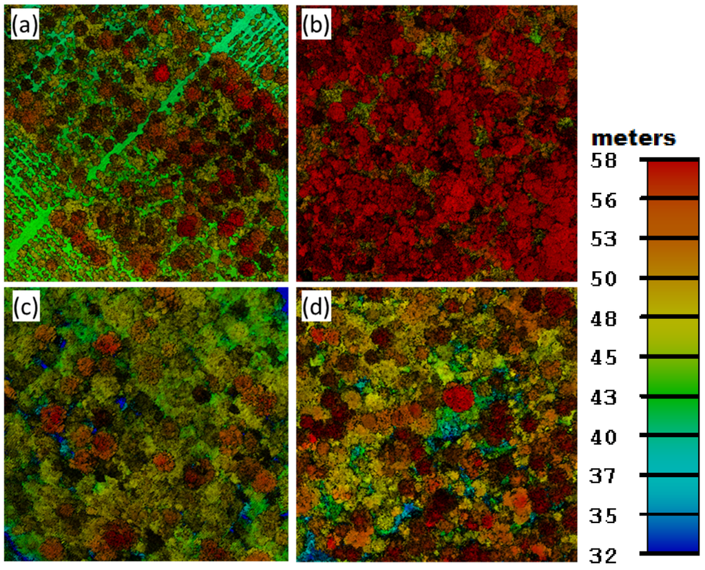
Figure 2. Examples (a–d) of agroforestry (left) and forests (right) fields shown in airborne lidar. Color (from red to blue) represents the elevation of the laser points.

Figure 2. Examples (a–d) of agroforestry (left) and forests (right) fields shown in airborne lidar. Color (from red to blue) represents the elevation of the laser points.

Figure 3. Teak plantations shown in the field (a); aerial photo (b); and lidar data (c); American oil palm sample tree (d); and plantation shown in aerial photos (e); and lidar data (f).

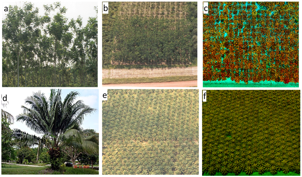
Figure 3. Teak plantations shown in the field (a); aerial photo (b); and lidar data (c); American oil palm sample tree (d); and plantation shown in aerial photos (e); and lidar data (f).

4. Results

With the multiplicative power model and our feature selection procedure, the final plot-level AGB prediction model is a simple power model based on the 90th percentile height:

$${\widehat{B}}_{plot}=13.94\ast H_{90th}^{0.86}$$

(7)

The model R² is 0.47 and the RMSE is 60.4 Mg/ha (see Figure 4a). Note that the mean AGB of all plots is 105.2 Mg/ha, which means that the coefficient of variation (CV) or relative prediction error is almost 60%. In particular, we found that plots 10 and 11 have relatively large residuals. Plot 11 is in an American oil palm plantation. The large residual of plot 11 is mainly caused by the unique DBH-H relationship of American oil palm trees, which implies that the AGB of American oil palm needs to be modeled separately from other vegetation types (see Section 5.1). However, we had only one plot of American oil palm, which eliminates the possibility of independently assessing the model prediction errors. Thus, plot 11 was excluded in our analysis, and the corresponding AGB model (see Figure 4b) developed after feature selection was:

$${\widehat{B}}_{plot}=8.28\ast H_{80th}^{1.06}$$

(8)

where H_80th is the 80th percentile height of lidar points.

Figure 4. Models for predicting plot-level AGB with the American oil palm plot included (a) and excluded (b); and the relationship between residual and wood density at the plot level (c).

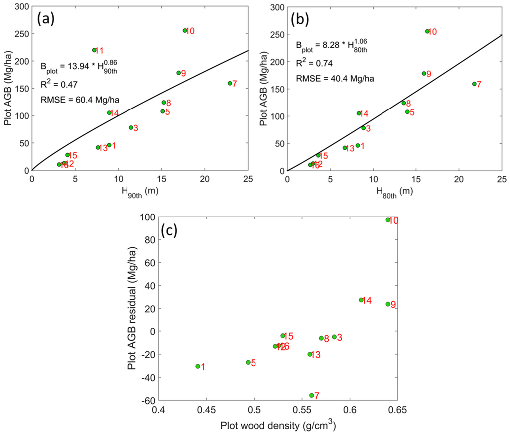
Figure 4. Models for predicting plot-level AGB with the American oil palm plot included (a) and excluded (b); and the relationship between residual and wood density at the plot level (c).

Note that when the allometric model for non-palm trees (Equation (2)) was used to estimate AGB, wood density is an important variable. As shown in Table 2, the teak plantation plots (plots 9 and 10) have the highest plot-level wood density. Plot 14 also has high average wood density because some of the species within it, such as ameixa and goiaba have high wood density (see Table 1 and Table 2). The large plot-level wood density of these three plots can explain why they all have positive residuals in AGB prediction models (Figure 4b).

The patterns revealed in the residual errors of plot-level AGB model prediction (i.e., plots with large wood density led to large positive residuals) (Figure 4c) suggest that the residuals are not statistically independent, i.e., an obvious violation of the basic assumption of the ordinary least squares (OLS) regression models. A statistical approach that can naturally consider the correlation within individual observations is mixed-effects models. The idea of mixed-effects models is to stratify the observations (i.e., plots in this study) into different groups and allow the model parameters vary as realizations of random variables across the groups. By doing so, the residuals of model prediction within individual groups will become more statistically independent. Mixed-effects models provide a trade-off between fitting all data points with one model and fitting models for each group independently. Hence it is well suited for handling data with few observations within groups [50].

The use of mixed-effects models requires the grouping of individual plots. The relatively large wood density of plots 9, 10, 14, and their positive residuals in the fixed-effects model imply that these three plots can be put into one group. The teak plantations (plots 9 and 10) not only have high wood density but also have the potential of being mapped over large area from remotely sensed data. Thus, we also tried to put only plots 9 and 10 into one group. As a result, we consider two different grouping scenarios as shown in Table 3. As shown in Equation (8), the developed fixed-effects model was a simple power model (in the form of y = a*x^b, where a and b are model parameters) with the 80th percentile height of lidar points as the predictor. In all of our mixed-effects modeling experiments, we found that only the parameter $b$ had statistically significant random effects. Therefore, in the mixed-effects models, only the parameter $b$ varies with vegetation groups. For grouping scheme A, the model parameters a = 8.63, b₁ = 1.15, and b₂ = 0.98, where b₁ and b₂ are the parameters for groups 1 and 2, respectively. For grouping scheme B, the model parameters a = 7.23, b₁ = 1.22, and b₂ = 1.03. Note that here the mixed-effects model for a given grouping scheme is equivalent to two simple power models for the two vegetation groups within the scheme (Figure 5).

Table 3. Different schemes of grouping plots for developing mixed-effects models.

Scheme	Group#1	Group#2
A	Teak plantation (plot 9, 10)	Non-teak (other plots)
B	High wood density plots (plot 9, 10, 14)	Other (other plots)

Table 3. Different schemes of grouping plots for developing mixed-effects models.

Scheme	Group#1	Group#2
A	Teak plantation (plot 9, 10)	Non-teak (other plots)
B	High wood density plots (plot 9, 10, 14)	Other (other plots)

When we used the same plots for calibration and validation (i.e., re-substitution), the R² was much higher and RMSE was much smaller when we used mixed-effects models in comparison to fixed-effects models (Table 4). The increase of goodness-of-fit in these statistics was expected because mixed-effects models are more complex (i.e., more parameters) than fixed-effects models. AIC is a statistic that penalizes the increase of model fitness due to the use of more complex models [51]. When we fitted mixed-effects models based on two groups, the AIC values decreased slightly for scheme A and by about four for scheme B (note that lower AIC values are preferred for modeling). Figure 5 shows the lidar-based AGB models developed from the field plots as well as their AGB prediction in comparison to the field-based estimates.

We also used leave-one-out cross-validation for calculating R² and RMSE to further assess the models’ prediction performance (Table 4). We found that the fixed-effects model had R² as low as 0.38, which was increased to 0.64 and 0.75 when mixed-effects models with scheme A and scheme B were used. This confirms the importance of stratification and mixed-effects modeling for predicting AGB.

Table 4. Comparison of fixed-effects and mixed-effects models for plot-level AGB estimation.

Model Type	Re-Substitution			Cross-Validation
	R2	RMSE (Mg/ha)	AIC	R2	RMSE (Mg/ha)
Fixed-effects model
	0.74	40.4	122.6	0.38	56.4
Mixed-effects model
Scheme A	0.91	25.9	122.0	0.64	42.9
Scheme B	0.94	21.6	118.7	0.75	35.9

Table 4. Comparison of fixed-effects and mixed-effects models for plot-level AGB estimation.

Model Type	Re-Substitution			Cross-Validation
	R2	RMSE (Mg/ha)	AIC	R2	RMSE (Mg/ha)
Fixed-effects model
	0.74	40.4	122.6	0.38	56.4
Mixed-effects model
Scheme A	0.91	25.9	122.0	0.64	42.9
Scheme B	0.94	21.6	118.7	0.75	35.9

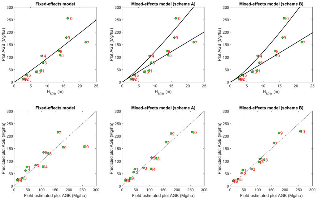
Figure 5. Comparison of fixed-effects and mixed-effects models for estimating plot AGB. The solid lines in the first-row figures are model curves. The dashed lines in the second-row figures are 1:1 line.

Figure 5. Comparison of fixed-effects and mixed-effects models for estimating plot AGB. The solid lines in the first-row figures are model curves. The dashed lines in the second-row figures are 1:1 line.

Figure 6 shows vegetation distribution 6a and the estimated AGB 6b and 6c over the whole agroforestry area using mixed- and fixed-effects models, respectively. The mean AGB densities estimated from fixed- and mixed-effects models were 57.0 Mg/ha and 51.7 Mg/ha, respectively. So, the average AGB density estimate from fixed-effects models was about 10% higher than the one from mixed-effects model. Moreover, by checking the spatial pattern of their difference at the pixel level (Figure 6d), we can see that the teak plantation AGB was underestimated by up to ~70 Mg/ha (or 33%) while the other agroforestry AGB were overestimated by up to ~60 Mg/ha (or 25%) using fixed-effects models in comparison to mixed-effects models.

Figure 6. Maps of vegetation type (a); and AGB predicted with mixed-effects model (b); and fixed-effects model (c); and the difference between AGB predicted with fixed- and mixed-effects models (d). Black color indicates the area masked for analysis.

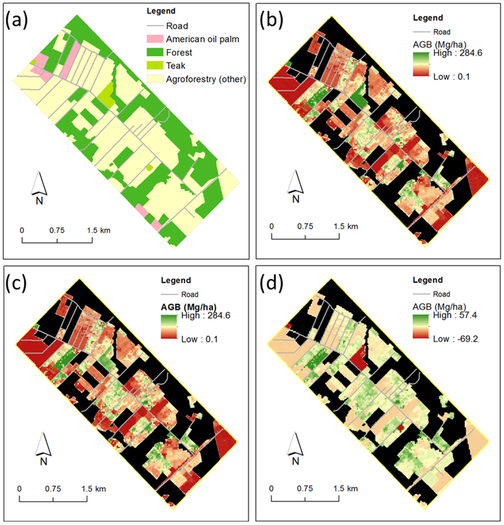
Figure 6. Maps of vegetation type (a); and AGB predicted with mixed-effects model (b); and fixed-effects model (c); and the difference between AGB predicted with fixed- and mixed-effects models (d). Black color indicates the area masked for analysis.

5. Discussion

5.1. Tree DBH-H Relationship

Note that, according to the allometric models used in this study (i.e., Equations (1) and (2)), DBH is the only predictor for estimating palm trees’ AGB and the major factor for predicting other trees’ AGB. However, lidar is more suited for estimating vegetation height than for DBH because the latter usually has to be indirectly estimated from airborne lidar data via its statistical relationship with lidar height metrics. When such allometric models are used, the capability of predicting AGB from lidar is governed by the strength of tree-level DBH-H relationship.

Figure 7 shows the relationship between DBH and tree height for all species based on the field measurements. It is clear that the tree-level data points can be separated into two groups. The group at the right includes 13 American oil palm trees, all from plot 11. Although the other tree species in this study exhibits positive relationship between DBH and height, the American oil palms do not show such a pattern. This might be due to the fact that the plants grow by increasing its diameter rather than height after reaching a certain size. As a result, the American oil palms have unique DBH-H relationship compared to most other tree species in this study. Note that the plot-level AGB model (i.e., Equation (7)) was calibrated to fit AGB from all plots while American oil palms exists in only plot 11. Hence, it is not surprising that the model (see Figure 4a) has large prediction error for the American oil palm plot. The unique DBH-H relationship of American oil palm suggested that it should be treated separately in our modeling. However, we were concerned that the model was not reliable with just one such plot. As a result, we decided to exclude the American oil palm plot in our further analysis.

Figure 7. DBH and tree height (H) relationships for American oil palm and other tree species.

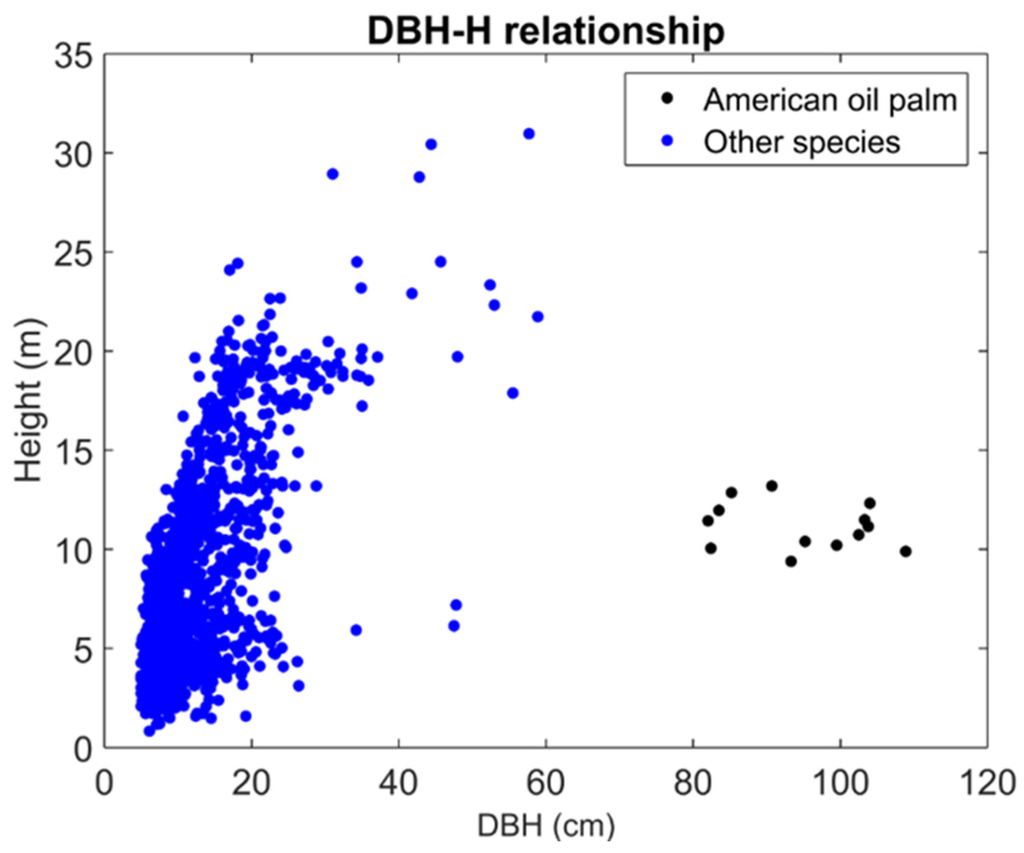
Figure 7. DBH and tree height (H) relationships for American oil palm and other tree species.

5.2. Allometry

One of the biggest uncertainties in our analysis is the tree-level AGB allometric models, especially for palms. For example, Goodman et al. [52] developed an allometric model for Euterpe precatoria, which is the allometric model that we could find and is the closest to our acai palm species (Euterpe oleracea). However, when the model (${\widehat{B}}_{tree} \left(kg\right)=13.589\ast H_s-108.81$) was applied to our acai palms, 235 out of 287 trees had negative AGB estimates. That allometric model was developed with 8 trees with a limited DBH range of 12–19 cm. Nevertheless, 242 Acai trees in this study have DBH < 12 cm. The small number and the limited range of the size for trees that were used to calibrate the model [52] can explain the failure of applying such a model into our study area. Unfortunately, no other allometric models specifically for acai palms were found in the literature. We do not have quantitative information about the errors of applying general allometric models (i.e., Equation (1)) to predict the AGB of the palm species in our study. More than 2000 species of palm trees occur in the world. Palm is the most abundant arborescent plant family in western Amazonian forest [52]. Thus, improving our knowledge about the AGB allometry for palms trees, in addition to dicotyledonous trees, is critical for accurate estimation of the AGB and carbon stock in Amazon.

Tree AGB allometric models are key to quantify the errors of remotely sensed AGB. It has been increasingly recognized that it is crucial to characterize the uncertainty of AGB estimates at the pixel and larger spatial scales [36,53,54,55]. The RMSE based on leave-one-out cross validation only characterized the errors related to the lidar-based AGB models, without considering errors related to tree AGB allometry, model parameters, field measurements, and lidar data. Chen et al. [36] did a comprehensive study of different error sources of AGB prediction when airborne lidar data and field data were combined to model and map AGB in an African tropical forest. It was found that errors related to tree AGB allometry and lidar-based regression models were the two major error sources in pixel-level AGB estimates. One of the cornerstones of that study is the availability of the destructively measured tree AGB for characterizing the error of tree AGB allometric models. Although we can apply that methodology to characterize AGB prediction errors for dicotyledonous trees in this study, palms need separate allometric models [52]. Unfortunately, the lack of access to the destructive AGB measurements for palm trees prevents us from fully assessing the errors of agroforestry AGB in this study.

5.3. Mixed-Effects Modeling

A limitation of this study is the small sample size (n = 12) for plot-level AGB modeling. We used mixed-effects models to address the dependence of lidar-AGB relationship on vegetation type and that left us with small numbers of plots per vegetation type. We should use the developed models for AGB prediction for other areas with caution, especially when there are out of the range of the input variables. In the future, more field plots ought to be collected, especially for American oil palm and teak plantations, to develop AGB models for larger areas. The one-year time difference between the times of lidar and field data acquisitions could also contribute to the errors in AGB prediction.

The use of the mixed-effects models for spatially-explicit AGB mapping requires the classification of the agroforestry fields over the whole study area based on their corresponding grouping schemes. Although we found that the grouping scheme B had the best prediction accuracy (Table 4), this model is more challenging to use in our study area because it requires the identification of high wood density areas. The calculation of the average wood density over an area depends on mapping of individual tree species, which is difficult for polyculture agroforestry fields that have multilayer canopy structure. Instead, we chose grouping scheme A for vegetation type classification because teak plantations can be more easily recognized from remotely sensed data owing to the relatively uniform and simple canopy structure (Figure 3a–c). Preliminary results from a supervised classification using 5-m RapidEye satellite imagery (unpublished data) indicated that teak plantations could be classified with a user accuracy and producer accuracy of 97.7% and 96.4%, respectively. Therefore, our methodology, when combined with digital classification of remotely sensed data, has potential to be applied and extended over large areas. One future research direction is to apply object-based image analysis (OBIA) approach and/or hyperspectral imagery to improve the classification of agroforestry fields [56,57,58].

We excluded forests to stay focused in the study of agroforestry. As shown earlier, it was difficult to separate agroforestry field and forests when an agroforestry field is dense and mixed with many tree species (see Figure 2c,d). A remaining question is whether it is necessary to separate agroforestry and forests in such cases. In other words, it is unclear whether AGB for forests and such agroforestry fields can be fit using just one model. One cold answer this question with comparable field and lidar data over forest and agroforestry plots.

6. Conclusions

Agroforestry has great potential for carbon sequestration while providing multiple benefits to individual farmers and communities. This study examined the potentials and challenges of using airborne lidar data for estimating AGB in an agroforestry system in the Brazilian Amazon. Several significant lessons were learned.

(1)

We found strong evidence to support the stratification of vegetation types in agroforestry fields for AGB modeling and mapping. This is in contrast to the widespread use of statistical models with no awareness of different vegetation types in most studies of tropical forest AGB using airborne lidar. Different from forests where trees are selected or adapted via natural processes, the trees in agroforestry are selected and planted by people to maximize economic and other benefits on purpose. Thus, the trees in agroforestry systems usually show more spatially-regularized patterns with a few co-occurring species. The species and structural diversities within agroforestry fields are usually smaller than the ones within forests while the diversities across different agroforestry fields may be larger. Therefore, the need for stratifying vegetation types in agroforestry is stronger than in forests for AGB studies.

(2)

This study analyzed the residual errors resulted from regular fixed-effects models and found that the errors have a pattern related to the variations in plot-level wood density. Based on this pattern, agroforestry fields were classified for lidar-based AGB modeling. This is an improvement over previous studies (e.g., [50]) that used existing vegetation classification schemes not specifically developed for lidar-based AGB modeling and mapping.

(3)

This study reinforced the utility of mixed-effects models for biomass modeling and mapping. Mixed-effects models can naturally incorporate how different species or groups have different wood densities and thus distinct lidar height—tree AGB relationships. Mixed-effects models also can elegantly cope with the issue of small sample size via adjustment of model parameters as a combination of fixed and random effects. With the classification of agroforestry into teak plantations and other types, we found the mixed-effects models improved the R² of AGB prediction from 0.38 to 0.64 and reduced the RMSE from 56.4 Mg/ha to 42.9 Mg/ha in comparison to fixed-effects models. We expect this study will encourage the further use of this under-investigated tool in the community of remote sensing of biomass and carbon.

This study highlighted the lack of reliable AGB allometry models, especially for palms, to comprehensively quantify the errors of lidar-based AGB estimates. This study also suggested the need to collect more field data over larger areas for automated mapping of plantation types and improved AGB modeling and mapping.

References

- Nair, P.R. An Introduction to Agroforestry; Kluwer Academic Publishers: Dordrecht, The Netherlands, 1993. [Google Scholar]
- Negash, M.; Kanninen, M. Modeling biomass and soil carbon sequestration of indigenous agroforestry systems using CO2FIX approach. Agric. Ecosyst. Environ. 2015, 203, 147–155. [Google Scholar] [CrossRef]
- Zomer, R.J.; Trabucco, A.; Coe, R.; Place, F. Trees on Farms: Analysis of the Global Extent and Geographical Patterns of Agroforestry; ICRAF Working Paper No. 89; World Agroforestry Centre: Nairobi, Kenya, 2009. [Google Scholar]
- Mbow, C.; van Noordwijk, M.; Luedeling, E.; Neufeldt, H.; Minang, P.A.; Kowero, G. Agroforestry solutions to address food security and climate change challenges in Africa. Curr. Opin. Environ. Sustain. 2014, 6, 61–67. [Google Scholar] [CrossRef]
- Albrecht, A.; Kandji, S.T. Carbon sequestration in tropical agroforestry systems. Agric. Ecosyst. Environ. 2003, 99, 15–27. [Google Scholar] [CrossRef]
- Thorlakson, T.; Neufeldt, H.; Dutilleul, F.C. Reducing subsistence farmers’ vulnerability to climate change: Evaluating the potential contributions of agroforestry in western Kenya. Agric. Food Secur. 2012, 1, 1–13. [Google Scholar] [CrossRef]
- Nguyen, Q.; Hoang, M.H.; Öborn, I.; van Noordwijk, M. Multipurpose agroforestry as a climate change resiliency option for farmers: An example of local adaptation in Vietnam. Clim. Change 2013, 117, 241–257. [Google Scholar] [CrossRef]
- McNeely, J.A. Nature vs. nurture: Managing relationships between forests, agroforestry and wild biodiversity. Agrofor. Syst. 2004, 61, 155–165. [Google Scholar]
- Jose, S. Agroforestry for conserving and enhancing biodiversity. Agrofor. Syst. 2012, 85, 1–8. [Google Scholar] [CrossRef]
- Ramos, N.C.; Gastauer, M.; de Cordeiro, A.A.C.; Meira-Neto, J.A.A. Environmental filtering of agroforestry systems reduces the risk of biological invasion. Agrofor. Syst. 2015, 89, 279–289. [Google Scholar] [CrossRef]
- Anderson, S.H.; Udawatta, R.P.; Seobi, T.; Garrett, H.E. Soil water content and infiltration in agroforestry buffer strips. Agrofor. Syst. 2009, 75, 5–16. [Google Scholar] [CrossRef]
- Hernandez, G.; Trabue, S.; Sauer, T.; Pfeiffer, R.; Tyndall, J. Odor mitigation with tree buffers: Swine production case study. Agric. Ecosyst. Environ. 2012, 149, 154–163. [Google Scholar] [CrossRef]
- Asbjornsen, H.; Hernandez-Santana, V.; Liebman, M.; Bayala, J.; Chen, J.; Helmers, M.; Ong, C.; Schulte, L. Targeting perennial vegetation in agricultural landscapes for enhancing ecosystem services. Renew. Agric. Food Syst. 2014, 29, 101–125. [Google Scholar] [CrossRef]
- Pandey, D.N. Carbon sequestration in agroforestry systems. Clim. Policy 2002, 2, 367–377. [Google Scholar] [CrossRef]
- Sharrow, S.H.; Ismail, S. Carbon and nitrogen storage in agroforests, tree plantations, and pastures in western Oregon, USA. Agrofor. Syst. 2004, 60, 123–130. [Google Scholar] [CrossRef]
- Kirby, K.R.; Potvin, C. Variation in carbon storage among tree species: Implications for the management of a small-scale carbon sink project. For. Ecol. Manag. 2007, 246, 208–221. [Google Scholar] [CrossRef]
- Nair, P.K.R. Carbon sequestration studies in agroforestry systems: A reality-check. Agrofor. Syst. 2012, 86, 243–253. [Google Scholar] [CrossRef]
- Lorenz, K.; Lal, R. Soil organic carbon sequestration in agroforestry systems: A review. Agron. Sustain. Dev. 2014, 34, 443–454. [Google Scholar] [CrossRef]
- Smith, P.; Bustamante, M.; Ahammad, H.; Clark, H.; Dong, H.; Elsiddig, E.A.; Haberl, H.; Harper, R.; House, J.; Jafari, M.; et al. Agriculture, Forestry and Other Land Use (AFOLU). In Climate Change 2014: Mitigation of Climate Change. Contribution of Working Group III to the Fifth Assessment Report of the Intergovernmental Panel on Climate Change; Edenhofer, O., Pichs-Mdruga, R., Sokana, Y., Minx, J.C., Farahani, E., Kadner, S., Seyboth, K., Adler, A., Baum, I., Brunner, S., et al., Eds.; Cambridge University Press: Cambridge, UK; New York, NY, USA, 2014. [Google Scholar]
- Skole, D.L.; Samek, J.H.; Chomentowski, W.; Smalligan, M. Forest, carbon, and the global environment: New directions in research. In Land Use and the Carbon Cycle: Advances in Integrated Science, Management, and Policy; Brown, D.G., Robinson, D.T., French, N.H.F., Reed, B.C., Eds.; Cambridge University Press: New York, NY, USA, 2013. [Google Scholar]
- Lu, D.; Chen, Q.; Wang, G.; Liu, L.; Li, G.; Moran, E. A survey of remote sensing-based aboveground biomass estimation methods in forest ecosystems. Int. J. Digit. Earth 2014. [Google Scholar] [CrossRef]
- Bolfe, É.L.; Batistella, M.; Ferreira, M.C. Correlation of spectral variables and aboveground carbon stock of agroforestry systems. Pesqui. Agropecu. Bras. 2012, 47, 1261–1269. [Google Scholar] [CrossRef]
- Czerepowicz, L.; Case, B.S.; Doscher, C. Using satellite image data to estimate aboveground shelterbelt carbon stocks across an agricultural landscape. Agric. Ecosyst. Environ. 2012, 156, 142–150. [Google Scholar] [CrossRef]
- Mitchard, E.T.A.; Meir, P.; Ryan, C.M.; Woollen, E.S.; Williams, M.; Goodman, L.E.; Mucavele, J.A.; Watts, P.; Woodhouse, I.H.; Saatchi, S.S. A novel application of satellite radar data: Measuring carbon sequestration and detecting degradation in a community forestry project in Mozambique. Plant Ecol. Divers. 2013, 6, 159–170. [Google Scholar] [CrossRef]
- Dube, T.; Mutanga, O. Investigating the robustness of the new Landsat-8 Operational Land Imager derived texture metrics in estimating plantation forest aboveground biomass in resource constrained areas. ISPRS J. Photogramm. Remote Sens. 2015, 108, 12–32. [Google Scholar] [CrossRef]
- Chen, Q. Lidar remote sensing of vegetation biomass. In Remote Sensing of Natural Resources; Wang, G., Weng, Q., Eds.; CRC Press/Taylor and Francis: Boca Raton, FL, USA, 2013; pp. 399–420. [Google Scholar]
- Montesano, P.M.; Nelson, R.F.; Dubayah, R.O.; Sun, G.; Cook, B.D.; Ranson, K.J.R.; Næsset, E.; Kharuk, V. The uncertainty of biomass estimates from LiDAR and SAR across a boreal forest structure gradient. Remote Sens. Environ. 2014, 154, 398–407. [Google Scholar] [CrossRef]
- Margolis, H.A.; Nelson, R.F.; Montesano, P.M.; Beaudoin, A.; Sun, G.; Andersen, H.E.; Wulder, M. Combining Satellite Lidar, Airborne Lidar and Ground Plots to Estimate the Amount and Distribution of Aboveground Biomass in the Boreal Forest of North America. Can. J. For. Res. 2015, 45, 838–855. [Google Scholar] [CrossRef]
- McRoberts, R.E.; Næsset, E.; Gobakken, T.; Bollandsås, O.M. Indirect and direct estimation of forest biomass change using forest inventory and airborne laser scanning data. Remote Sens. Environ. 2015, 164, 36–42. [Google Scholar] [CrossRef]
- Latifi, H.; Fassnacht, F.; Koch, B. Forest structure modeling with combined airborne hyperspectral and LiDAR data. Remote Sens. Environ. 2012, 121, 10–25. [Google Scholar] [CrossRef]
- Chen, Q. Modeling aboveground tree woody biomass using national-scale allometric methods and airborne lidar. ISPRS J. Photogramm. Remote Sens. 2015, 106, 95–106. [Google Scholar] [CrossRef]
- Asner, G.P.; Clark, J.K.; Mascaro, J.; Galindo García, G.A.; Chadwick, K.D.; Navarrete Encinales, D.A.; Paez-Acosta, G.; Montenegro, E.C.; Kennedy-Bowdoin, T.; Duque, Á.; et al. High-resolution mapping of forest carbon stocks in the Colombian Amazon. Biogeosciences 2012, 9, 2683–2696. [Google Scholar] [CrossRef]
- D’Oliveira, M.V.; Reutebuch, S.E.; McGaughey, R.J.; Andersen, H.E. Estimating forest biomass and identifying low-intensity logging areas using airborne scanning lidar in Antimary State Forest, Acre State, Western Brazilian Amazon. Remote Sens. Environ. 2012, 124, 479–491. [Google Scholar] [CrossRef]
- Andersen, H.E.; Reutebuch, S.E.; McGaughey, R.J.; d’Oliveira, M.V.; Keller, M. Monitoring selective logging in western Amazonia with repeat lidar flights. Remote Sens. Environ. 2014, 151, 157–165. [Google Scholar] [CrossRef]
- Vaglio Laurin, G.; Chen, Q.; Lindsell, J.A.; Coomes, D.A.; del Frate, F.; Guerriero, L.; Pirotti, F.; Valentini, R. Above ground biomass estimation in an African tropical forest with lidar and hyperspectral data. ISPRS J. Photogramm. Remote Sens. 2014, 89, 49–58. [Google Scholar] [CrossRef]
- Chen, Q.; Laurin, G.V.; Valentini, R. Uncertainty of remotely sensed aboveground biomass over an African tropical forest: Propagating errors from trees to plots to pixels. Remote Sens. Environ. 2015, 160, 134–143. [Google Scholar] [CrossRef]
- Yamada, M.; Gholz, H.L. An evaluation of agroforestry systems as a rural development option for the Brazilian Amazon. Agrofor. Syst. 2002, 55, 81–87. [Google Scholar] [CrossRef]
- Rodrigues, T.E.; dos Santos, P.L.; Rolim, P.A.M.; Santos, E.; Rego, R.S.; da Silva, J.M.L.; Valente, M.A.; Gama, J.R.N.F. Caracterização e Classificação dos Solos do Município de Tomé-Açu, Pará; Embrapa Amazônia Oriental: Belém, Pará, Brazil, 2001; p. 49. [Google Scholar]
- Homma, A.K.O. História da Agricultura na Amazônia: Da era Pré-Colombiana ao Terceiro Milênio; Embrapa Informação Tecnológica: Brasília, Distrito Federal, Brazil, 2003; p. 274. [Google Scholar]
- Homma, A.K.O. Dinâmica dos sistemas agroflorestais: O caso da Colônia Agrícola de Tomé-Açu, Pará. Rev. Inst. Estud. Super. Amazôn. 2004, 2, 57–65. [Google Scholar]
- Walker, W.; Baccini, A.; Nepstad, D.; Horning, N.; Knight, D.; Braun, E.; Bausch, A. Field Guide for Forest Biomass and Carbon Estimation, Version 1.0; Woods Hole Research Center: Falmouth, MA, USA, 2011. [Google Scholar]
- Keller, M.; Palace, M.; Hurtt, G. Biomass estimation in the Tapajos National Forest, Brazil: Examination of sampling and allometric uncertainties. For. Ecol. Manag. 2001, 154, 371–382. [Google Scholar] [CrossRef]
- Hunter, M.O.; Keller, M.; Victoria, D.; Morton, D.C. Tree height and tropical forest biomass estimation. Biogeosciences 2013, 10, 8385–8399. [Google Scholar] [CrossRef]
- Nascimento, H.E.; Laurance, W.F. Total aboveground biomass in central Amazonian rainforests: A landscape-scale study. For. Ecol. Manag. 2002, 168, 311–321. [Google Scholar] [CrossRef]
- Chave, J.; Réjou-Méchain, M.; Búrquez, A.; Chidumayo, E.; Colgan, M.S.; Delitti, W.B.; Duque, A.; Eid, T.; Fearnside, P.M.; Goodman, R.C.; et al. Improved allometric models to estimate the aboveground biomass of tropical trees. Glob. Change Biol. 2014. [Google Scholar] [CrossRef] [PubMed]
- Chave, J.; Coomes, D.; Jansen, S.; Lewis, S.L.; Swenson, N.G.; Zanne, A.E. Towards a worldwide wood economics spectrum. Ecol. Lett. 2009, 12, 351–366. [Google Scholar] [CrossRef] [PubMed]
- Zanne, A.E.; Lopez-Gonzalez, G.; Coomes, D.A.; Ilic, J.; Jansen, S.; Lewis, S.L.; Miller, R.B.; Swenson, N.G.; Wiemann, M.C.; Chave, J. Global Wood Density Database. Dryad. Available online: http://hdl.handle.net/10255/dryad, 235 (accessed on 21 September 2015).
- Fathi, L. Structural and Mechanical Properties of the Wood from Coconut Palms, Oil Palms and Date Palms. Ph.D. Thesis, University of Hamburg, Hamburg, Germany, 2014. [Google Scholar]
- Chen, Q. Airborne lidar data processing and information extraction. Photogramm. Eng. Remote Sens. 2007, 73, 109–112. [Google Scholar]
- Chen, Q.; Laurin, G.V.; Battles, J.J.; Saah, D. Integration of airborne lidar and vegetation types derived from aerial photography for mapping aboveground live biomass. Remote Sens. Environ. 2012, 121, 108–117. [Google Scholar] [CrossRef]
- Chen, Q.; Gong, P.; Baldocchi, D.; Tian, Y.Q. Estimating basal area and stem volume for individual trees from lidar data. Photogramm. Eng. Remote Sens. 2007, 73, 1355–1365. [Google Scholar] [CrossRef]
- Goodman, R.C.; Phillips, O.L.; del Castillo Torres, D.; Freitas, L.; Cortese, S.T.; Monteagudo, A.; Baker, T.R. Amazon palm biomass and allometry. For. Ecol. Manag. 2013, 310, 994–1004. [Google Scholar] [CrossRef]
- Wang, G.; Oyana, T.; Zhang, M.; Adu-Prah, S.; Zeng, S.; Lin, H.; Se, J. Mapping and spatial uncertainty analysis of forest vegetation carbon by combining national forest inventory data and satellite images. For. Ecol. Manag. 2009, 258, 1275–1283. [Google Scholar] [CrossRef]
- Lu, D.; Chen, Q.; Wang, G.; Moran, E.; Batistella, M.; Zhang, M.; Laurin, G.V.; Saah, D. Aboveground forest biomass estimation with Landsat and LiDAR data and uncertainty analysis of the estimates. Int. J. For. Res. 2012. [Google Scholar] [CrossRef]
- McRoberts, R.E.; Westfall, J.A. Effects of uncertainty in model predictions of individual tree volume on large area volume estimates. For. Sci. 2014, 60, 34–42. [Google Scholar] [CrossRef]
- Lu, D.; Hetrick, S.; Moran, E. Land cover classification in a complex urban-rural Landscape with QuickBird imagery. Photogramm. Eng. Remote Sens. 2010, 76, 1159–1168. [Google Scholar] [CrossRef]
- Bigdeli, B.; Samadzadegan, F.; Reinartz, P. A decision fusion method based on multiple support vector machine system for fusion of hyperspectral and LIDAR data. Int. J. Image Data Fusion 2014, 5, 196–209. [Google Scholar] [CrossRef]
- Ghamisi, P.; Benediktsson, J.A.; Phinn, S. Land-cover classification using both hyperspectral and LiDAR data. Int. J. Image Data Fusion 2015, 6, 189–215. [Google Scholar] [CrossRef]
© 2015 by the authors; licensee MDPI, Basel, Switzerland. This article is an open access article distributed under the terms and conditions of the Creative Commons by Attribution (CC-BY) license (http://creativecommons.org/licenses/by/4.0/).