
Short-Term Forecasting of Surface Solar Irradiance Based on Meteosat-SEVIRI Data Using a Nighttime Cloud Index

Abstract
: The cloud index is a key parameter of the Heliosat method. This method is widely used to calculate solar irradiance on the Earth’s surface from Meteosat visible channel images. Moreover, cloud index images are the basis of short-term forecasting of solar irradiance and photovoltaic power production. For this purpose, cloud motion vectors are derived from consecutive images, and the motion of clouds is extrapolated to obtain forecasted cloud index images. The cloud index calculation is restricted to the daylight hours, as long as SEVIRI HR-VIS images are used. Hence, this forecast method cannot be used before sunrise. In this paper, a method is introduced that can be utilized a few hours before sunrise. The cloud information is gained from the brightness temperature difference (BTD) of the 10.8 µm and 3.9 µm SEVIRI infrared channels. A statistical relation is developed to assign a cloud index value to either the BTD or the brightness temperature T10.8, depending on the cloud class to which the pixel belongs (fog and low stratus, clouds with temperatures less than 232 K, other clouds). Images are composed of regular HR-VIS cloud index values that are used to the east of the terminator and of nighttime BTD-derived cloud index values used to the west of the terminator, where the Sun has not yet risen. The motion vector algorithm is applied to the images and delivers a forecast of irradiance at sunrise and in the morning. The forecasted irradiance is validated with ground measurements of global horizontal irradiance, and the advantage of the new approach is shown. The RMSE of forecasted irradiance based on the presented nighttime cloud index for the morning hours is between 3 and 70 W/m2, depending on the time of day. This is an improvement against the previous precision range of the forecast based on the daytime cloud index between 70 and 85 W/m2.1. Introduction
With the steadily increasing contribution of photovoltaic (PV) power to the electricity mix in Europe and especially in Germany, reliable predictions of the expected PV power production are becoming increasingly important as a basis for power and grid management and operation strategies. PV power has to be offered on the auctions at the European Power Exchange [1]. At noon, the electricity is traded for the following day (day-ahead) in 24-hour intervals, requiring hourly PV power forecasts for the next day. On the intraday market, electricity contingents of 15-minute periods may be traded until 45 minutes before delivery begins. This allows for an adaptation of the day-ahead schedule to forecast updates with 15-minute resolution up to several hours ahead, which can be more accurate than the day-ahead forecasts. The remaining deviations between scheduled and needed power are adjusted by using balancing energy and reserve power on the very short-term timescale. As this is very costly, the high accuracy of the PV power forecasts is essential for cost-efficient grid integration [2].
The accuracy of forecasted PV power is reliant on the accuracy of the forecasted surface solar irradiance. Irradiance forecasts based on cloud motion vector fields from satellite images perform significantly better than forecasts of numerical weather prediction systems for short-term horizons of up to four hours; see Kühnert et al. [3]. For the calculation of surface irradiance, the Heliosat method is implemented in the forecasting routine. The Heliosat method extracts cloud information from the brightness-normalized HR-VIS (high-resolution visible wavelengths) channel. This method has two shortcomings: before sunrise, the lack of information in the dark regions of the HR-VIS images makes short-term forecasts impossible; shortly after sunrise, for high solar zenith angles, the uncertainty of the method increases due to an over-brightening of the normalized HR-VIS digital counts. A cloud product that is continuous over the day and night transition (solar terminator) could solve the problem of lacking early morning forecasts. In particular, during the winter, the quality and availability of short-term forecasts for the intraday energy market could be increased significantly.
For nighttime cloud and fog detection, the 10.8–3.9 µm brightness temperature difference (BTD) is commonly used [4–7]. It is defined as:
At night, this brightness temperature difference for a cloud free pixel is caused by the difference in surface spectral emissivity ϵ(λ) observed at both wavelengths. Emissivities for different surface types for the Northern Hemisphere have been derived from MODIS data by Chen et al. [8]. For natural surfaces, the 3.7 µm emissivity is always smaller than the 10.8 µm emissivity. The smallest emissivity difference ∆ϵ is found for water (∆ϵ ≈ 0.01); most of the land surfaces show slightly higher values for ∆ϵ between 0.02 and 0.05, while for barren or sparsely-vegetated surfaces, the emissivity difference is as high as 0.17.
Based on radiative transfer calculations, Hunt calculated emissivity differences for different wavelengths for water and ice clouds [9]. For clouds with small droplets, as found in fog and low stratus, and an optical thickness of 10, the emissivity at 3.8 µm is notably lower than at 11 µm (∆ϵ between 0.2 and 0.4). The emissivity difference is much higher than for most surfaces, except for sandy deserts. Thus, this feature is used for the detection of fog and low water clouds [10].
Ice clouds contain larger particles. Here, Hunt found only small emissivity differences between the near-infrared and infrared wavelengths. Nevertheless, semi-transparent ice-clouds have a higher transmittance at 3.9 µm, which means that the contribution of the relatively warm ground is higher at the 3.9 µm brightness temperature than at 10.8 µm (T3.9 > T10.8). With the resulting BTD, these clouds can be separated from the cloud-free case, as well as from fog and low stratus clouds.
Both classes of clouds can be distinguished from the cloudless ground by using threshold tests. These tests are only applied at night, when the solar irradiance does not affect the 3.9-µm channel radiance. Moreover, the high radiometric noise occurring in the 3.9-µm channel of the Meteosat SEVIRI instrument at low temperatures constrains the method to pixels warmer than 240 K [4]. For the detection of these clouds, the cloud-free surface BTD has to be estimated for the different surface emissivities and the prevailing atmospheric absorption. For the operational detection of high semi-transparent clouds or low water clouds, brightness temperature thresholds are pre-calculated with radiative transfer calculations for variable water vapor content and different satellite viewing angles. The results are filed in look-up tables for warm and cold ocean, land and desert surfaces [4].
As stated by Cermak and Bendix, the instrument design of Meteosat SEVIRI leads to a BTD that depends on the satellite viewing angle [11]. The SEVIRI 3.9-µm band is exceptionally wide and overlaps with the 4-µm CO2 absorption band. Therefore, the SEVIRI BTD shows an offset of 4 K compared with other radiometers. In addition, the brightness temperature difference varies with the length of the slant atmospheric column between sensor and object (limb cooling) and the varying concentrations of CO2. To account for these effects, the authors have presented a dynamic extraction of BTD thresholds for different satellite viewing angles.
Several authors have worked on the development of cloud products that are continuous across the terminator. Gustafson and d’Entremont use the BTD for both day and night cloud detection [12]. Since the 3.9-µm band consists of reflected solar radiation during daytime in addition to Earth’s thermal emission, different thresholds for daytime and nighttime are needed for cloud detection. Gustafson and d’Entremont employ a linear interpolation of these thresholds within the twilight zone to provide a continuous cloud product. Derrien and Le Gléau have improved low cloud detection from SEVIRI data at twilight by taking advantage of these clouds’ persistent temporal characteristic [13]. Mosher combines a brightness-normalized visible image during the day and a synthetic nighttime visible image for continuous cloud visualization [14]. The synthetic part of the image is derived with linear stretching from the BTD values for fog and low stratus and from brightness temperature values T10.8 for high clouds above 18,000 feet. The result is a gray-level image having the same approximate appearance in the nighttime part as in the daytime part. As the images are meant to be operationally used in aviation, the higher clouds are given a blue color.
The approach presented in this paper offers a continuous cloud product and is inspired by Mosher’s approach to use BTD values for fog and low stratus and brightness temperature values T10.8 for other clouds. However, here, a quantitative measure for cloud transmission is derived, which can be used to calculate surface solar irradiance. For this purpose, the Heliosat cloud index during daytime is used, and for the night, a cloud index from either BTD or T10.8 IR values is calculated. In addition, a statistical approach is developed that maps the IR values to the cloud index value range according to their cumulative distributions. This non-linear relation is trained for the three different classes “fog and low stratus”, “clouds with temperatures less than 232 K” and “other clouds”. The satellite viewing angle is accounted for to avoid the limb cooling observed in SEVIRI BTD. This enables the use of uniform thresholds within the European image section when assigning clouds to these three classes. The classification is based on the viewing angle corrected BTD values.
This paper briefly describes the Heliosat method to derive a conventional cloud index and the global horizontal irradiance from daytime HR-VIS SEVIRI images. The main focus of this paper lies on the description of the new approach and the calculation of the presented nighttime cloud index. A forecasting routine is applied to nighttime cloud index images to obtain global horizontal irradiance for horizons of up to eight hours. The direct validation of the nighttime cloud index is not possible. Therefore, the method is validated using the forecasted global horizontal irradiance. The uncertainties of the Heliosat method, e.g., in mountain regions or in situations with snow coverage or changing atmospheric turbidity, are not analyzed here, but considered as a reference uncertainty. The main focus of the validation is to study if the introduction of the nighttime cloud index improves the forecasting of surface solar irradiance.
2. Data and Method
2.1. Satellite Data
The Meteosat Second Generation (MSG) satellites carry the Spinning Enhanced Visible and Infrared Imager (SEVIRI), which observes the Earth using 12 spectral channels. The satellite images cover Europe, the North Atlantic and Africa and are acquired every 15 minutes. The channels cover wavelengths between 0.6 µm and 14 µm with one high-resolution broadband visible channel (HR-VIS, 0.3–0.7 µm). The spatial resolution at the sub-satellite point is 1 km × 1 km for HR-VIS and 3 km × 3 km for the other channels. The pixels in these images contain brightness information as 10-bit digital counts. For the derivation of the cloud index, the HR-VIS imagery after sunrise and the two infrared channels at 3.9 µm and 10.8 µm before sunrise are used. Clouds and snow have a similar brightness in the HR-VIS imagery. Nevertheless, it is possible to distinguish between both during daytime by calculating a normalized differential snow index from the visible channel at 0.6 µm and the near-infrared channel at 1.6 µm and applying temporal variability and temperature tests.
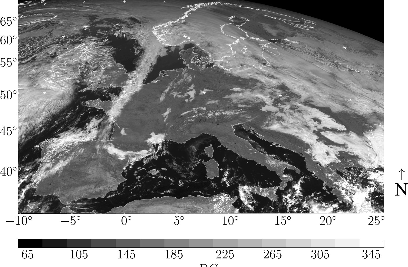
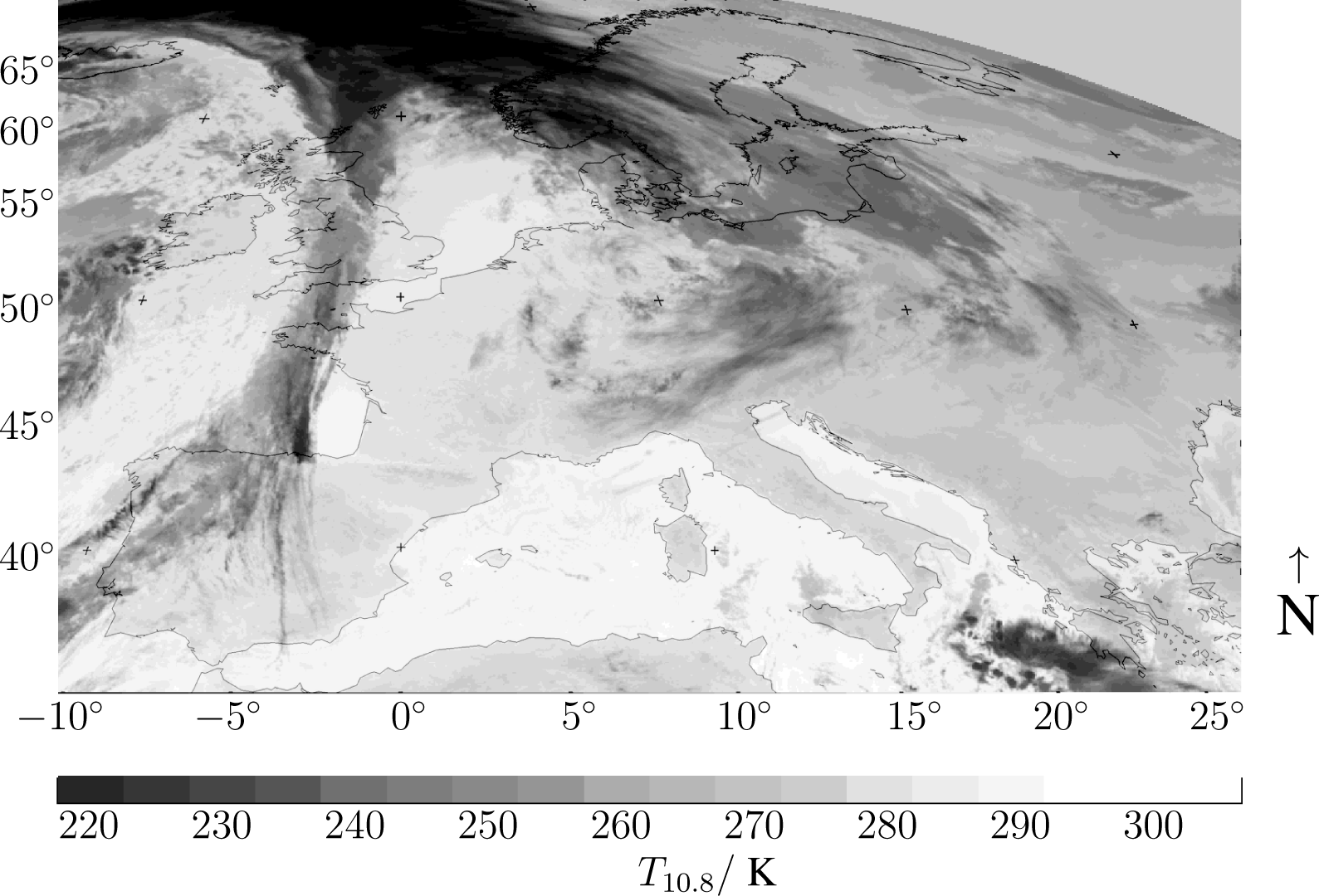
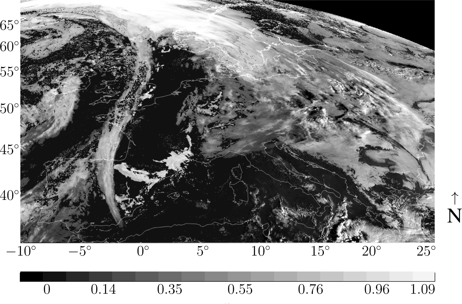
At the University of Oldenburg, forecasts of surface solar irradiance and photovoltaic power are calculated for application at the German electricity market. For this purpose, satellite images of Europe are used. The size of the high-resolution images is 1800 lines by 3072 columns. In Figures 1 and 2, examples of an HR-VIS image and an IR image are shown for the spatial area under consideration. The IR images are scaled to the same resolution as the HR-VIS images to create a continuous series of cloud index images for the entire day, including the time before sunrise.
The database used for this paper consists of images of the year 2013 for the development of the method and of the months September 2014–February 2015 for application and validation. This winter was nearly snow free in Germany, besides a few days in early February. For this reason, the application of the snow detection algorithm has not been considered within the validation study.
2.2. Cloud Index
The Heliosat method was originally proposed by Cano et al. [15]. For Meteosat Second Generation satellites, a modified version is used at the University of Oldenburg; see Hammer et al. [16]. The MSG HR-VIS digital counts C are normalized with respect to the solar zenith angle θ. These brightness-normalized digital counts are also known as relative reflectance ρ:
Here, C is the digital count (measured pixel brightness) of the satellite radiometer and C0 is the instrument offset.
The observed reflectance ρ is low for most types of Earth surfaces and high for clouds. Using this fact, the cloud index n as a measure of the cloud cover is introduced:
To find the reference value of relative surface reflectance ρg for each pixel, a statistical analysis of the darkest pixels is performed on a monthly basis. The calculation is done twice a week using the previous 30 days to account for seasonal variations of the surface reflectance. The reference values for cloud reflectance ρc are dependent on the sun-satellite geometry. Therefore, for each season, a set of ρc has been determined from frequency distributions of ρ for classes with similar geometric configurations.
The cloud index varies between n ≈ 0 for cloud-free and n ≈ 1 for overcast conditions. The cloud index for each pixel is stored as a 10-bit brightness value with a digital count value range from DC = 0 for n = −0.2 to DC = 1023 for n = 1.2. Snow is usually misinterpreted as a cloud within the Heliosat method. For this reason, snow detection is performed with the other MSG SEVIRI channels. In the case of snow and cloudless sky, the cloud index is assigned n = −0.15 and for clouds above snow n = 0.5.
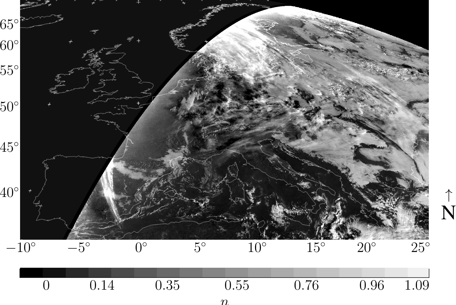
An example of the Heliosat cloud index is given in Figure 3. In this image, the western part is not illuminated, so no cloud index values can be assigned to the pixels. An over-brightening close to the terminator line is visible. Apart from this, the image contains pure cloud information in contrast to the surface features visible in Figure 1.
The reason of the over-brightening in cloud index images at sunrise (and sunset) lies in the normalization of visible counts in Equation (2). The expression for the airmass X = 1/cosθ exceeds all limits when the zenith angle θ approaches 90°, i.e., when the Sun is located just above the horizon. To avoid this effect, the airmass function given by Rozenberg [17] is introduced here:
With an airmass correction of X = 40 for θ = 90°, Equation (4) is applicable at sunrise. In twilight situations with the Sun below the horizon (θ > 90.77° and X > 64), the authors of this paper use X = 64 as an upper limit in the normalization function. Airmass definitions by other authors are given in Table 1.
2.3. Clear Sky Index and Global Horizontal Irradiance
Within the Heliosat method, the cloud index is linked to the clear sky index. The clear sky index k*∗ is defined by normalizing the actual global horizontal irradiance I with the clear sky irradiance Iclear:
Here, the clear sky irradiance is estimated with the Dumortier clear sky model [19] using the turbidity given in [20] for Europe. The clear sky index k* can be calculated from the cloud index n as follows [21]:
With Equation (6), the global horizontal irradiance I = k* · Iclear can be calculated from the cloud index n for each pixel. While the transmission of clouds is handled by the clear sky index, the atmospheric turbidity due to aerosol and water vapor content and the elevation of the site are included in the clear sky model. An independent validation of the hourly global irradiance calculated with the implementation of the Heliostat method used within this paper but using the worldwide turbidity given in [22] has been performed by Ineichen [23]. Data from 18 sites, including up to eight years of ground measurements, have been used. The relative mean bias deviation resulted in −0.8%, and the standard deviation was 17%.
2.4. Brightness Temperature Difference
The digital count (brightness) of each pixel in SEVIRI’s infrared images can be converted into the spectral radiance R by using the calibration information given in the metadata of SEVIRI images [24]. Depending on the infrared channel, these radiances are further converted to equivalent brightness temperatures T3.9 and T10.8 following the equations and parameters given by Eumetsat [25].
In this paper, in contrast to Equation (1), the brightness temperature difference BTD is defined as:
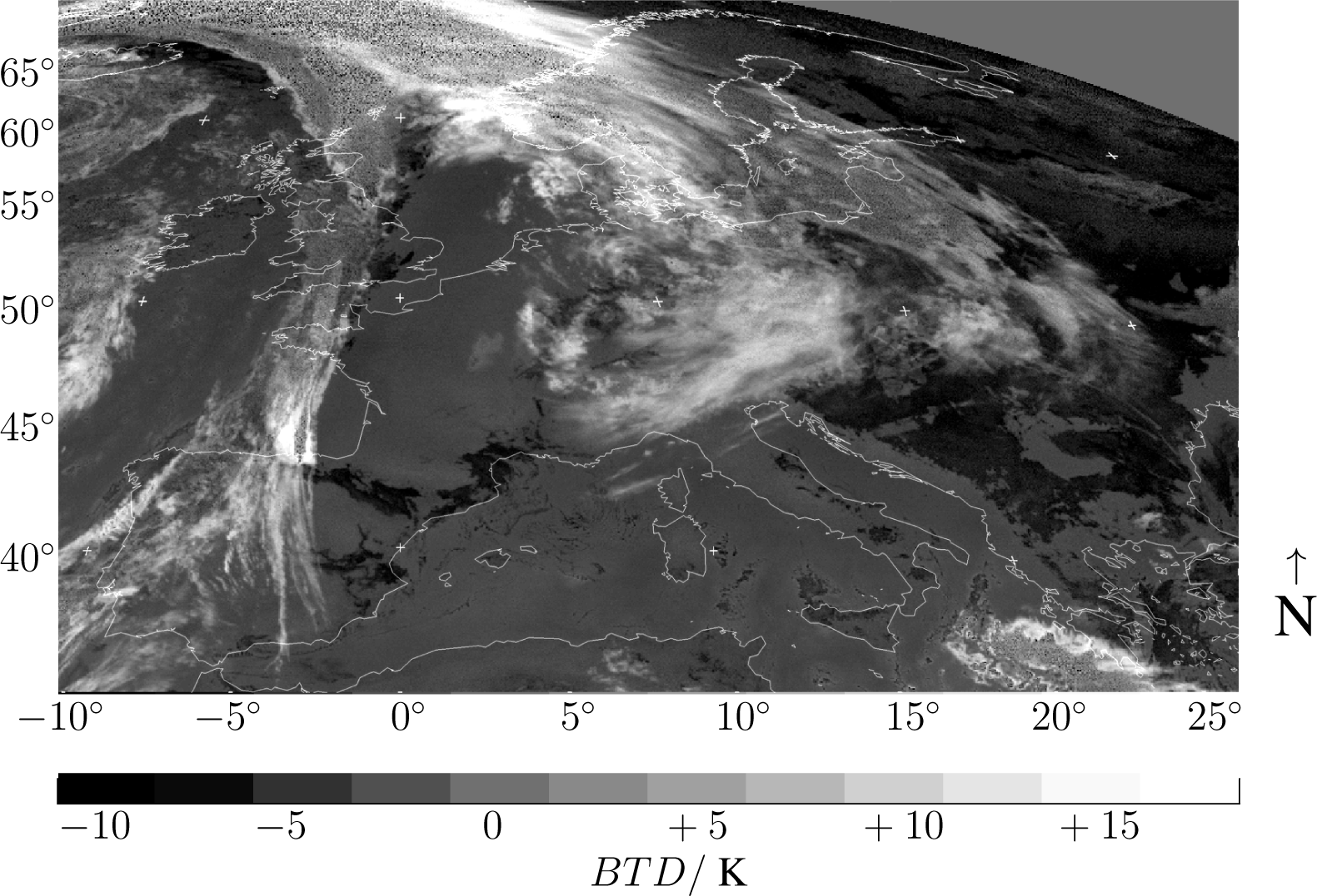
With this definition and the spectral emissivity and transmissivity differences explained in the Introduction, fog and low stratus clouds have a BTD lower than land surface or ocean. All other clouds have a higher BTD than land or ocean. An example of a BTD image is given in Figure 4. The image noise in the upper left part is due to the 3.9-μm radiometric noise occurring at low temperatures. At the same time, these low temperatures are represented as dark areas in Figure 2.
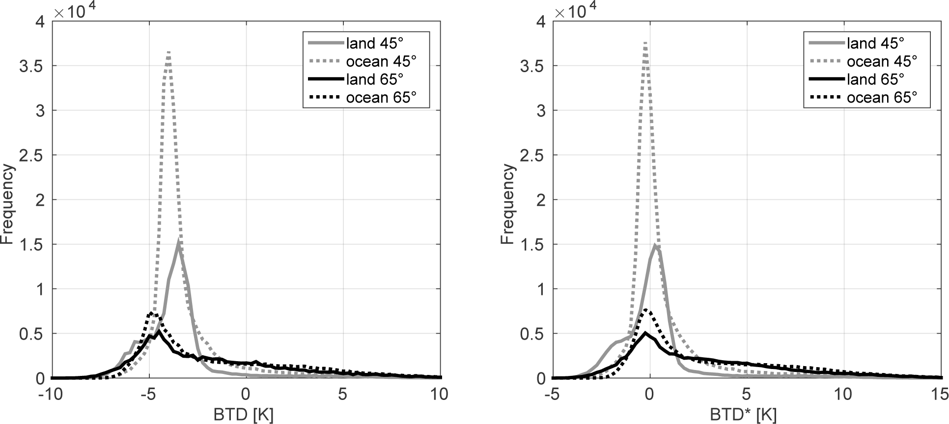
In Figure 5, left panel, the frequency distribution of brightness temperature differences is shown for the European image section for 11 January 2013, 03:00 UTC. The frequency distributions are shown separately for land and ocean pixels for two exemplary intervals of satellite viewing angles v, specified by 40° ≤ v < 50° and 60° ≤ v < 70°. The ocean and land pixels have been separated by a land mask precalculated from cloudless pixels in the SEVIRI 0.6 µm channel.
The resulting four histograms each show BTD values between −10 K and +10 K, each with a distinct peak representing cloudless pixels. Fog and low stratus pixels in the histogram are located to the left of the peak and all other clouds to the right. In this figure, the limb cooling effect is discernible: the cloudless peak lies at P = −5 K for the higher viewing angle and for the lower angle at Pocean = −4.0 K for ocean and Pland = −3.5 K for land pixels.
2.5. Viewing Angle Correction
To account for limb cooling, a viewing angle correction is applied to the brightness temperature difference. This makes it possible to define fixed thresholds for the distinction between cloudy and cloudless weather conditions. The correction function is found by observing the cloudless land and ocean peaks for different viewing angles.
Average values for the cloudless peak have been calculated from frequency distributions of 73 images in 2013. This database consists of one nighttime image every five days. The resulting averages and standard deviations for the cloudless land and ocean peaks are given in Table 2. The values for the ocean peaks have been used to find the linear fit for viewing angle correction:
This fit is used to calculate the viewing angle corrected brightness temperature difference:
For comparison, the fit results Pocean,fit are listed for five viewing angles in Table 2. The values slightly differ from the average ocean peaks, but lie well within the given standard deviation. A change in the viewing angle from 45° to 75° would result in a limb cooling of −1.1 K. This is in accordance with the empirically-developed correction for Europe given for this angle interval by [4].
The effect of Equations (8) and (9) is presented in Figure 5, right panel, in which the four histograms all peak around P = 0 K after application of the viewing angle correction. However, the corrected peaks for the entire image (histograms including all viewing zenith angles 30° ≤ v < 90°) for ocean and land differ from each other and from day to day. For these reasons, the cloudless land and ocean peaks Pland and Pocean are calculated for every night as cloudless reference values.
2.6. Cloud Classes
Satellite image pixels are sorted into cloud classes depending on the distance of their BTD* value to the cloudless peak P in the BTD* distribution and a given threshold δ that represents the width of the peak. If the distance exceeds the threshold δ, the pixel is assumed to be not clear, but cloudy.
Assuming normally-distributed values, the full width at half maximum FWHM of the peak is related to the standard deviation via σ = FWHM/2.3548. Further, 90% of all clear BTD* values fall within an interval of P ± δ around the cloudless peak with δ = 1.645 · σ, and 95% will fall within an interval with δ = 1.960 · σ.
The thresholds δ have been determined from the 0300 UTC images from March–December 2013. For these images, the frequency distributions of BTD* have been calculated. For all histograms with a cloudless land peak Pland or ocean peak Pocean with a high frequency of occurrence (>90.000), the average values of full width at half maximum FWHMocean and FWHMland have been calculated. Such high peaks have been found in 23 images for Pocean and 19 images for Pland. As a result of this approach, the standard deviations for the clear ocean have been found as σocean=0.46 K and for the clear land as σland = 0.53 K. For ocean, the 90% threshold has been chosen δocean = 0.76 K, and for land, the 95% threshold δland = 1.07 K, as the land emissivity values are more dispersed. Both thresholds are significantly smaller than the thresholds given in [7] 3.8 K for ocean and 3.5 K for land.
With these definitions and values, the cloud classes are defined as given in Table 3. The introduction of Class 3 is necessary because the BTD* cannot be used in a meaningful way for these very cold pixels. For the calculation of the nighttime cloud index, the BTD* can be utilized for pixels with brightness temperatures of T10.8 > 232 K; other authors set 240 K as the lower limit [4]. For clouds with T10.8 ≤ 232 K, the BTD* is influenced by radiometric noise on the 3.9-µm channel. For these clouds, the BTD* is not evaluated. Instead, these clouds are treated as a special class. Such very cold clouds have a very high optical thickness and, correspondingly, a very high cloud index.
For a given date, cloud classification is performed as follows: the two peaks Pocean and Pland are determined once for every night and used for cloud classification in all images of this night. The nightly recalculation of the peaks means that it is possible to follow seasonal trends in BTD* values due to changes in atmospheric content. The thresholds δocean and δland are considered as static values, which is in accordance with [6,7]. Nevertheless, as the narrower peaks have FWHM values of 0.5 K less than the wider peaks, there might be the potential for improvement in setting the thresholds. Improvements may lie in the use of seasonal thresholds or in considering the different spectral emissivities of land surface types.
2.7. Nighttime Cloud Index
The calculation of the nighttime cloud index nnight is performed on the four cloud classes introduced in the previous section. For cloud-free pixels (Class 0) a cloud index of nnight = 0 is assigned. For cloudy pixels, transformations are developed that assign the feature BTD* or T10.8 to a nighttime cloud index. To this end, the cumulative distribution F1 of brightness temperature difference BTD* is considered for fog and low stratus (lass 1), while the cumulative distributions F2 and F3 of temperature T10.8 are considered for the other clouds in Classes 2 and 3, respectively.
These nighttime distributions are derived in a resolution of 0.1 K. They are statistically related to the cumulative distributions N1, N2 and N2 of 10-bit cloud index n for the considered cloud class during daytime a few hours later. It is assumed that the clouds observed before sunrise are also visible in the daytime cloud index image a few hours later. It is further assumed that the majority of clouds may change their position within the image section, but maintain their distinctive features, like cloud index and spectral emissivity, within this period of time. Both assumptions are statistically fulfilled for images covering areas of continental dimensions as used in the method presented in this paper. Clouds entering or leaving the image frame are neglected, as well as clouds that change size or shape during the period of time.
For fog and low stratus, the statistical relation between BTD* and cloud index n has been determined with a database of 29 night and day image pairs of April 2013. Each of these pairs contains more than 500,000 cloudy pixels with BTD* < 0.5 K and T10.8 > 232 K at 0200 UTC and daytime cloud index nday > 0.1 at 0800 UTC. From all pixels that fulfill both conditions, the cumulative distributions F1(BTD*) and N1(nday) have been calculated. The following transformation maps each BTD* value to the daytime cloud index with the same quantile F1(BTD*) ≡ N1(nday); it uses the inverse of N1:
It is assumed that this transformation can also be used to assign a nighttime cloud index to the BTD* value. The resulting function f1 is a fit of the values shown in Figure 6, left panel. This estimation of the nighttime cloud index from BTD* is used whenever a pixel is classified as “fog and low stratus”.
Similarly, a cloud index is defined for the clouds in Classes 2 and 3 according to their temperature.
Following [14], the feature “temperature” is utilized for these clouds, as the dynamic range of their temperature is wider than the BTD* range. For this reason, it can be better compared to the cloud index range. For cloud Class 2, the transformation f2 is calculated for every day and used for the forecast of the next day for all clouds with T10.8 > 232 K. This procedure ensures that atmospheric temperature changes throughout the year are incorporated in the cloud index calculation.
For Class 3, a fixed relation is used, as such clouds do not occur every day. For the determination of the statistical relation between T10.8 and the cloud index n for this class, a month with a significant number of extremely cold clouds T10.8 < 232 K was chosen. In February 2013, these cold clouds occurred on 15 nights. In these nights, each 0300 UTC image contained more than 150,000 pixels of this cloud class. For these images, pixel pairs from two types of images were selected, consisting of the brightness temperature night value T10.8 at 0300 UTC and a daytime cloud index nday at 0800 UTC at the exact same location. The pixel pairs were chosen in such a way that T10.8,night < 232 K and T10.8,day < 242 K and, at the same time, nday > 0.35. This ensures that clouds that have moved from their night position are excluded from the dataset. The resulting function f3 is a fit of the values shown in Figure 6, right panel. This estimate of the nighttime cloud index from T10.8 is used whenever a pixel is classified as “very cold cloud”.
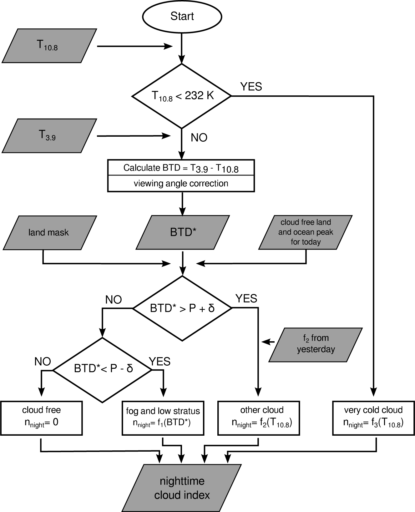
With the three Equations (10–12), it is possible to assign to each pixel a nighttime cloud index that is similar to the cloud index value during daytime. For pixels identified as belonging to Classes 1 and 3, the fixed relations shown in Figure 6 are used to calculate the nighttime cloud index nnight. The calculation of f2 for Class 2 is done dynamically once per day to follow temperature changes throughout the year. An overview of the new scheme is given in Figure 7.
2.8. Twilight and All-Day Cloud Index
With the definitions and equations given in the previous section for nnight and Equation (3) for nday, it is possible to calculate cloud index images for the entire day. Within the twilight zone, the cloud index is calculated as a weighted average of daytime and nighttime cloud index. The weights depend on the solar zenith angle for a given pixel. A similar approach was introduced in [12] for setting thresholds in the twilight zone. In this work, the twilight zone is defined by 85° < θ < 89.8°. Definitions by other authors are given in Table 1.
The all-day cloud index is calculated as:
The weights are defined by:
The combined day and night cloud index defined by Equations (13) and (14) is used as a basis for forecasting the global horizontal irradiance in the early morning. An example is given in Figure 8, where the night cloud index is seen in the western and the day cloud index in the eastern part of the image.
2.9. Short-Term Forecasting with Cloud Motion Vector Fields
The all-day cloud index images are the basis for short-term forecasting of global horizontal irradiance using cloud motion vectors (CMV). For the addressed forecast horizon, the evolution of cloud structures is most important. With the CMV forecast approach, the movement of clouds is predicted based on the current state. Forming and dissolving cloud structures are not considered by this approach. Motion vectors are calculated by comparing two consecutive cloud index images and represent the direction and speed of the clouds’ movement. Applied to the latest image, future cloud index images and, thus, surface irradiance are predicted. An additional smoothing post-processing increases forecast accuracy. A detailed description and analysis of CMV irradiance forecasts based on HR-VIS satellite images is given in [3].
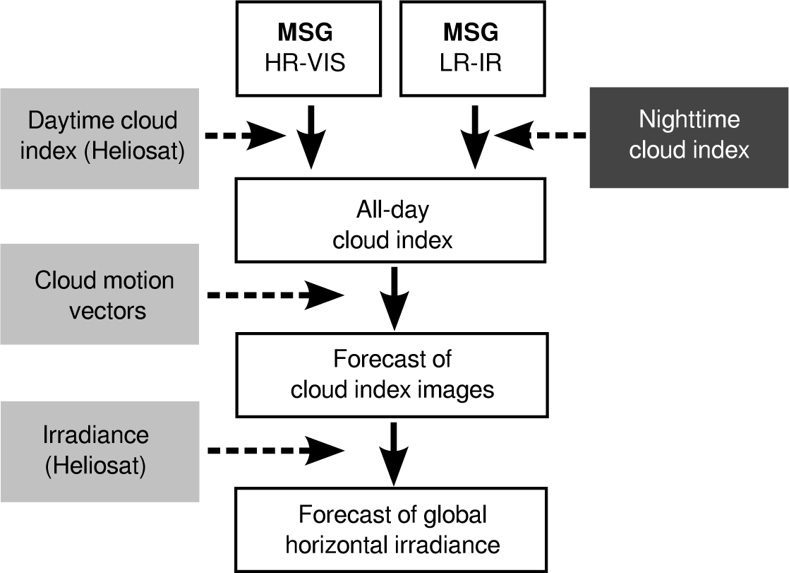
Figure 9 shows the irradiance forecast retrieval as presented here. All-day cloud index images are calculated with the Heliosat method for daytime images and with the BTD* method presented in this paper for nighttime images. The CMV method is applied to these images to forecast cloud index images and global horizontal irradiance.
2.10. Verification with Ground Measurements of Global Horizontal Irradiance
Measured surface global horizontal irradiance data are used to validate the presented method. The measured data are provided by the German Weather Service (DWD, Deutscher Wetterdienst) and by Meteogroup GmbH in an hourly resolution. A total of 116 sites distributed over Germany are included in the dataset, maintained by the corresponding provider regarding quality control and instrument calibration. Details on the measurement networks, instruments and the accuracies can be found in [26] and [27]. The dataset covers the months September 2014–February 2015.
To validate the presented method, the accuracy of predicting daytime global horizontal irradiance at these stations is derived by applying the CMV forecast method to the all-day cloud index images. The validation focuses on forecast lead times of two to three hours, since this time horizon is of high importance for application at the energy market. For the validation, RMSE and bias error measures are utilized. Forecasts using all-day cloud index images are compared to forecasts based on daytime cloud index images derived from the HR-VIS channel only. Additionally, irradiance derived with the Heliosat method is given for reference, being based on the daytime cloud index without forecast.
3. Results and Discussion
The nighttime cloud index is validated using CMV irradiance forecasts by extrapolating cloud information from nighttime to daytime when irradiance measurements are available.
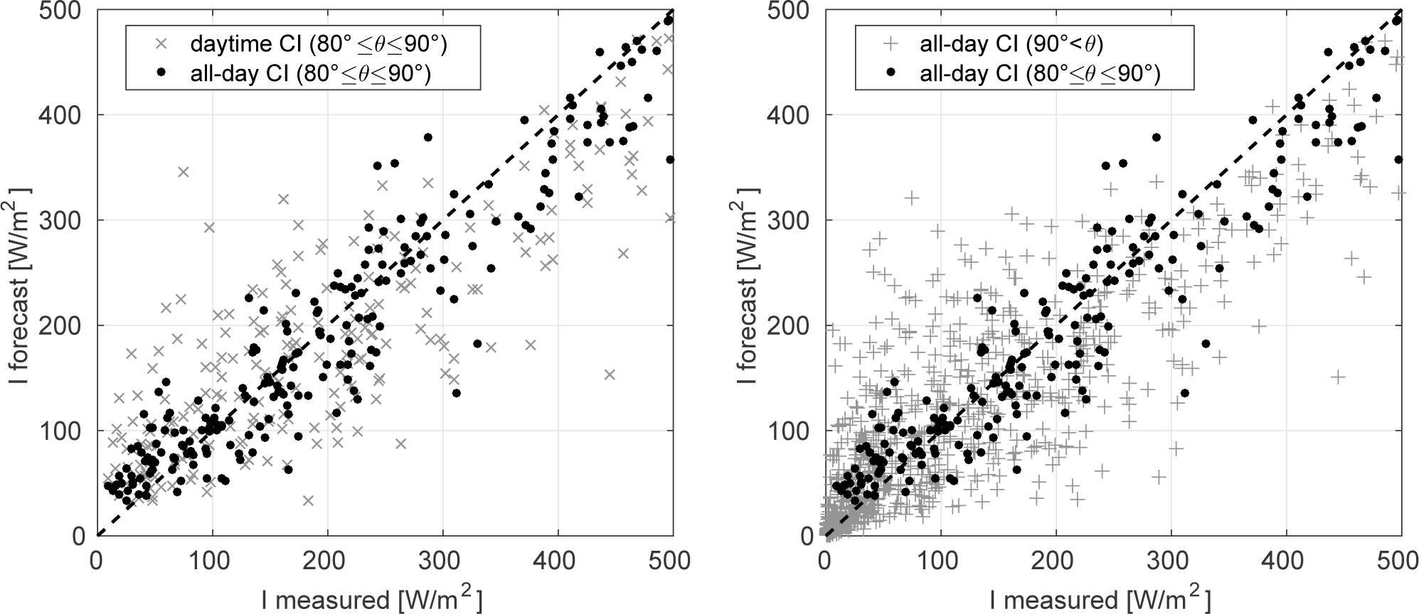
In Figure 10, the forecast accuracies of the presented BTD* based (“all-day”) forecasts and the established HR-VIS-based (“daytime”) forecasts are plotted for a single station. Only forecasts with solar zenith angle θ > 80° at forecast origin are displayed here. In the left panel of Figure 10, the impact of the Rozenberg airmass [17] on forecast quality is analyzed. The spread of the forecasts based on cloud index, including Rozenberg airmass, is significantly reduced compared to forecasts for the same situations using the cloud index values based on Equation (2) with unlimited airmass. Thus, the use of Equation (4) improves the performance of forecasts computed at solar zenith angles of 80° ≤ θ ≤ 90°.
By including the BTD* approach and, thus, making the CMV forecast computing at θ > 90° possible, the amount of available forecasts significantly increases, as can be seen in Figure 10 right. Still, a higher spread of predicted irradiance than compared to forecasts derived between 80° ≤ θ ≤ 90° is observed.
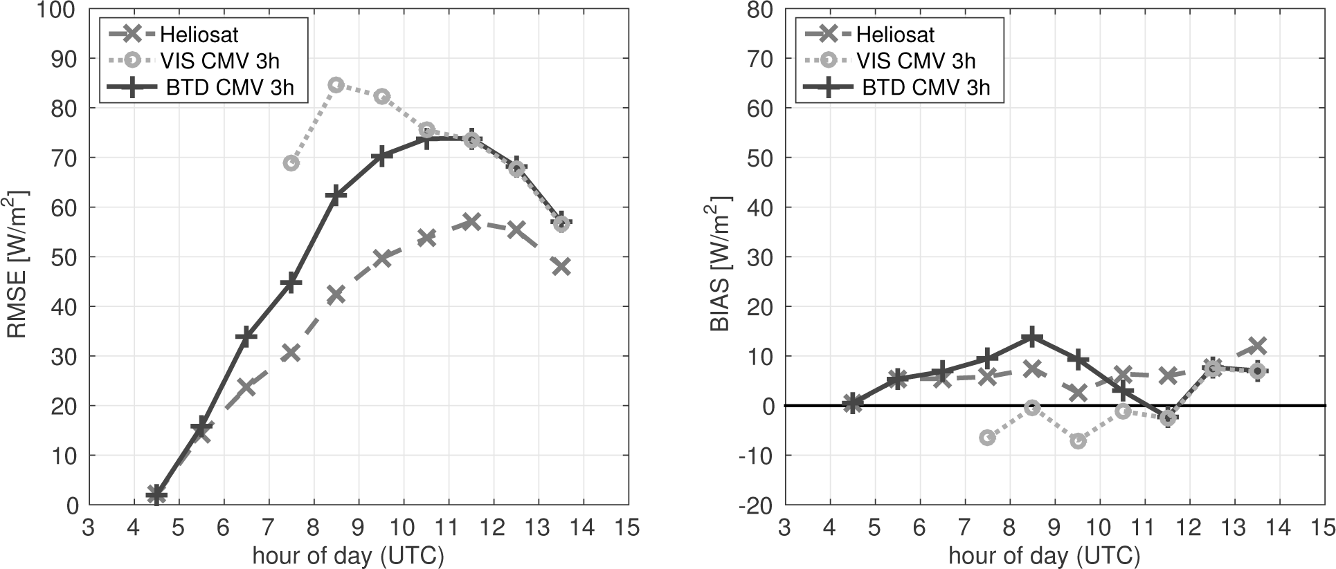
A quantification of the forecast accuracy for the complete dataset as described in Section 2.10 is displayed in Figure 11. RMSE and bias are compared for HR-VIS- and BTD*-based CMV forecasts with a three-hour lead time. The RMSE of the Heliosat method is displayed as a reference error for satellite-retrieved irradiance with no forecasting involved. The evaluation is performed with dependence on the time of day for forecasts originating before noon. The RMSE follows the diurnal course of global horizontal irradiance with the highest irradiance at noon and, thus, the highest RMSE values for these hours. According to the dataset evaluated, the average global horizontal irradiance reaches around 220 W/m2 at 1100 UTC, but only up to 80 W/m2 before 0800 UTC. This leads to a relative RMSE, normalized to the average measured I, of more than 50% for the morning hours and of around 30% at mid-day. The RMSE of the Heliosat method is regarded as the minimum RMSE of the CMV approach achievable and reaches up to around 60 W/m2 at noon.
The availability of HR-VIS channel-based CMV forecasts is limited in early morning hours. This is visible by a comparably small amount of available daytime cloud index-based forecasts in Figure 10 left. The earliest forecast possible in Figure 11 occurs several hours later than the first forecast possible with the all-day cloud index. Moreover, the cloud detection algorithm shows poor performance for forecasts computed at solar zenith angles θ ≥ 80° (see Figure 10 left) and Hours 7–10 in Figure 11, the latter corresponding to high solar zenith angles at the forecast origin for the winter months evaluated. In the evaluation presented here, the RMSE for morning hours ranges from 70 W/m2–85 W/m2 and reaches the same levels as for noon hours (around 75 W/m2).
With the BTD*-based approach presented, forecasts are available much earlier; they can now be computed at night and are available at sunrise (see Figure 10). For solar zenith angles 80° ≤ θ ≤ 90°, a significantly higher performance than of the HR-VIS-based forecast is observed. Here, RMSE values are between 45 and 70 W/m2 in the corresponding hours, compared to 70–85 W/m2 for HR-VIS-based forecasts for the same zenith angles. Still, as the resolution of the IR channels utilized is lower than for the HR-VIS channel and since the statistical transformation to cloud index values involves further uncertainty, forecast accuracy is not expected to reach the levels of forecasts derived at daytime. Later forecasts are identical, as both use HR-VIS images only.
The forecast bias is consistently positive for both BTD*-based forecasts with up to 15 W/m2 and the Heliosat method with up to 10 W/m2 in the displayed evaluation. Thus, a systematic overestimation is found, which indicates a general underestimation of cloud cover by the Heliosat method itself. For the HR-VIS-based forecasts, this positive bias is compensated by the opposite trend, induced by a significant over-brightening and, thus, overrating of cloud clover, as it is visible in the twilight zone (see Figure 3).
4. Conclusions
A new method has been presented to derive a nighttime cloud index from two infrared channels of the MSG SEVIRI instrument. The method is based on the brightness temperature difference commonly used in fog and low stratus detection during nighttime. For other clouds, a cloud index is assigned respecting their temperature. The resulting nighttime cloud index is the basis for short-term forecasts of global horizontal irradiance and photovoltaic power in the early morning hours. For these hours, short-term forecasts have not been possible before, as the Heliosat cloud index is derived from SEVIRI HR-VIS images, which contain no information before sunrise and imprecise information shortly after sunrise.
The precision range of forecasts (RMSE of global horizontal irradiance) based on the presented nighttime cloud index for the morning hours is between 3 and 70 W/m2, depending on the time of day. This is an improvement against the previous precision range of the forecast based on the daytime cloud index between 70 and 85 W/m2. This improvement demonstrates that the nighttime cloud index closes a significant gap in the availability of forecasts for the intraday energy market.
The method includes several new approaches: The viewing angle correction accounts for limb cooling observed in the brightness temperature differences and makes it possible to define constant thresholds to distinguish between cloudy and cloud-free situations. Two thresholds have been identified for land and water pixels. The identification of clouds is done dynamically using the distance of a pixel’s (viewing angle corrected) brightness temperature difference from that of a cloudless pixel. The cloudless cases differ for land and ocean and are identified as the most frequent brightness temperature difference values for the given night. Three cloud classes can be distinguished; for them, feature-preserving transformations have been introduced to assign a cloud index.
Future work will concentrate on the reduction of the bias of 15 W/m2, indicating an underestimation of cloud cover. Here, it will be studied if a narrower setting of the thresholds will result in the detection of more clouds and, thus, in a reduction of the bias. Further, as the emissivity of land surfaces is more variable than that of the ocean, it is foreseen to admit more land surface classes, to enable the identification of clouds with narrower thresholds.
Acknowledgments
This work has been supported by the German Federal Environmental Foundation DBU (Deutsche Bundesstiftung Umwelt) and the German Federal Ministry of Economics and Technology BMWi (Bundesministerium für Wirtschaft und Technologie). We thank the German Weather Service (DWD) and Meteogroup GmbH for providing global horizontal irradiance measurement data.
Author Contributions
Annette Hammer and Kailash Weinreich developed the method to derive a nighttime cloud index. Annette Hammer introduced the Rozenberg airmass and the twilight zone cloud index. Elke Lorenz developed the short-term forecast of solar irradiance using motion vector fields and the tables of reference values for cloud reflectance. Jan Kühnert implemented the nighttime cloud index in the forecasting scheme and performed the validation with ground measurements.
Conflicts of Interest
The authors declare no conflict of interest.
References
- European Power Exchange. Available online: http://www.epexspot.com/en/ accessed on 17 June 2015.
- Lorenz, E.; Kühnert, J.; Heinemann, D. Short term forecasting of solar irradiance by combining satellite data and numerical weather predictions, Proceedings of the 27th European PV Solar Energy Conference (EU PVSEC), Frankfurt, Germany, 24–28 September 2012; pp. 4401–4405.
- Kühnert, J.; Lorenz, E.; Heinemann, D. Satellite-based irradiance and power forecasting for the German energy market. In Solar Energy Forecasting and Resource Assessment; Kleissl, J., Ed.; Academic Press: Oxford, UK, 2013; pp. 267–297. [Google Scholar]
- Derrien, M.; le Gléau, H.; Fernandez, P. Algorithm Theoretical Basis Document for Cloud Products (CMa-PGE01v3.2, CT-PGE02 v2.2 & CTTH-PGE03v2.2); User Manual SAF/NWC/CDOP2/MFL/SCI/ATBD/01; EUMETSAT SAFNWC-Météo-France-Centre de Météorologie Spatiale: Lannion, France, 2013. Available online: http://www.nwcsaf.org/HTMLContributions/SUM/SAF-NWC-CDOP2-MFL-SCI-ATBD-01_v3.2.1.pdf accessed on 10 July 2015.
- Jedlovec, G. Automated detection of clouds in satellite imagery. Advances in Geoscience and Remote Sensing; Jedlovec, G., Ed.; InTech Europe: Rijeka, Croatia, 2009. Available online: http://www.intechopen.com/books/advances-in-geoscience-and-remote-sensing/automated-detection-of-clouds-in-satellite-imagery accessed on 10 July 2015. [Google Scholar] [CrossRef]
- Eumetsat, Cloud Detection for MSG—Algorithm Theoretical Basis Document EUM/MET/REP/07/0132; Eumetsat: Darmstadt, Germany, 2007.
- Hocking, J.; Francis, P.; Saunders, J. Cloud Detection in Meteosat Second Generation Imagery at the Met Office; Forecasting R&D Technical Report No. 40; Met Office: Exeter, UK, 2010. [Google Scholar]
- Chen, Y.; Sun-Mack, S.; Minnis, P.; Smith, W.L.; Young, D.F. Surface spectral emissivity derived from MODIS data. Proc. SPIE 2003, 4891, 361–369. [Google Scholar]
- Hunt, G.E. Radiative properties of terrestrial clouds at visible and infra-red thermal window wavelengths. Q. J. R. Meteorol. Soc. 1973, 99, 346–369. [Google Scholar]
- Ellrod, G.P. Advances in the detection and analysis of fog at night using GOES multispectral infrared imagery. Wea. Forecast. 1995, 10, 606–619. [Google Scholar]
- Cermak, J.; Bendix, J. Dynamical nighttime fog/low stratus detection based on Meteosat SEVIRI data: A feasibility study. Pure Appl. Geophys. 2007, 164, 1179–1192. [Google Scholar]
- Gustafson, G.; d’Entremont, R. Cloud detection and property retrieval across the day/night terminator, Proceedings of the 14th Conference on Satellite Meteorology and Oceanography, Atlanta, GA, USA, 29 January–2 February 2006.
- Derrien, M.; Le Gléau, H. Temporal-differencing and region-growing techniques to improve twilight low cloud detection from SEVIRI data, Proceedings of the Joint 2007 EUMETSAT Meteorological Satellite Conference and the 15th Satellite Meteorology and Oceanography Conference of the American Meteorological Society, Amsterdam, The Netherlands, 24–28 September 2007; pp. 24–28.
- Mosher, F.R. Day/Night Visible Satellite Images; Embry-Riddle Aeronautical University: Daytona Beach, FL, USA, 2006. Available online: http://works.bepress.com/frederick_mosher/7/ accessed on 10 July 2015.
- Cano, D.; Monget, J.; Albuisson, M.; Guillard, H.; Regas, N.; Wald, L. A method for the determination of the global solar radiation from meteorological satellite data. Sol. Energy 1986, 37, 31–39. [Google Scholar]
- Hammer, A.; Heinemann, D.; Hoyer, C.; Kuhlemann, R.; Lorenz, E.; Müller, R.W.; Beyer, H.G. Solar energy assessment using remote sensing technologies. Remote Sens. Environ. 2003, 86, 423–432. [Google Scholar]
- Rozenberg, G.V. Twilight: A Study in Atmospheric Optics; Plenum Press: New York, NY, USA, 1966. [Google Scholar]
- Li, J.; Shibata, K. On the effective solar pathlength. J. Atmos. Sci. 2006, 63, 1365–1373. [Google Scholar]
- Dumortier, D. Modelling Global and Diffuse Horizontal Irradiances under Cloudless Skies with Different Turbidities; Final Report JOU2-CT92-0144, Daylight II; École Nationale des Travaux Publics de l’État: Vaulx-en-Velin, France, 1995. [Google Scholar]
- Dumortier, D. The Satellight Model of Turbidity Variations in Europe; Report for the Sixth Satellight Meeting; École Nationale des Travaux Publics de l’État: Vaulx-en-Velin, France, 1998. [Google Scholar]
- Rusen, S.E.; Hammer, A.; Akinoglu, B.G. Estimation of daily global solar irradiation by coupling ground measurements of bright sunshine hours to satellite imagery. Energy 2013, 58, 417–425. [Google Scholar]
- Remund, J. Aerosol Optical Depth and Linke Turbidity Climatology; Description for Final Report of IEA SHC Task 36; Meteotest: Bern, Germany, 2009. [Google Scholar]
- Ineichen, P. Long Term Satellite Hourly, Daily and Monthly Global, Beam and Diffuse Irradiance Validation. Interannual Variability Analysis; IEA Report; University of Geneva: Geneva, Switzerland, 2013. [Google Scholar]
- Schmetz, J.; Pili, P.; Tjemkes, S.; Just, D.; Kerkman, J.; Rota, S.; Ratier, A. SEVIRI calibration. Bull. Amer. Meteorol. Soc. 2002, 83, ES52–ES53. [Google Scholar]
- Tjemkes, S.; Stuhlmann, R.; Hewison, T.; Müller, J. The Conversion from Effective Radiance to Equivalent Brightness Temperature; Technical Document EUM/MET/TEN/11/0569; Eumetsat: Darmstadt, Germany, 2012. [Google Scholar]
- Deutscher Wetterdienst DWD. Eingesetzte Sensorik an den Wetterwarten und Wetterstationen. Available online: http://www.dwd.de/sensorik accessed on 17 June 2015.
- Meteogroup Deutschland GmbH. Wetterstationen Deutschland, Available online: http://wetterstationen.meteomedia.de/ accessed on 17 June 2015.


| Author | Twilight Zone | Airmass | Limit |
|---|---|---|---|
| This work | 85° < θ < 89.8° | X = 1/(cosθ + 0.025 exp(−11 cosθ)) Rozenberg [17] | X < 64 |
| Météo-France [4] | 80° <θ<93° | X=1/cosθ | – |
| Eumetsat [6] | 80° <θ<95° | X=1/cosθ | – |
| Hocking et al. [7] | 80° <θ<90° | X=1/cosθ | – |
| X = 1/cos(85°) + 2.29 • (0 − 85°), if 0 > 85° | |||
| Gustafson and d’Entremont [12] | 80° < θ < 105° | empirical correction from GOES imagery, visible channel forθ≤99° similar to Rozenberg [17] | X<8 |
| Derrien and Le Gléau [13] | – | Li et al. [18] | X<24 |
| Mosher [14] | – | X=1/cosθ·1/(1+θ/180°) | – |
| Viewing Angle ν | Ocean BTD peak Pocean / K | Land BTD peak Pland / K | Pocean,fit/K |
|---|---|---|---|
| 30° ≤ v < 40° | −3.55 ± 0.91 | −3.38 ± 0.36 | −3.51 |
| 40° ≤ v < 50° | −3.72 ± 0.89 | −3.50 ± 0.28 | −3.81 |
| 50° ≤ v < 60° | −4.15 ± 0.59 | −3.66 ± 0.39 | −4.16 |
| 60° ≤ v < 70° | −4.65 ± 0.67 | −4.68 ± 1.02 | −4.56 |
| 70° ≤ v < 90° | −5.18 ± 0.88 | −4.88 ± 1.59 | −5.22 |
| Cloud Class | Constraint | |
|---|---|---|
| 0 | “cloud free” | P − δ < BTD* < P + δ |
| 1 | “fog and low stratus” | BTD*< P − δ |
| 2 | “other clouds” | P + δ<BTD* |
| 3 | “very cold clouds” | T10.8 < 232 K, BTD*∗ influenced by noise |
| δocean = 0.76 K, δland = 1.07 K | ||
© 2015 by the authors; licensee MDPI, Basel, Switzerland This article is an open access article distributed under the terms and conditions of the Creative Commons Attribution license (http://creativecommons.org/licenses/by/4.0/).
Share and Cite
Hammer, A.; Kühnert, J.; Weinreich, K.; Lorenz, E. Short-Term Forecasting of Surface Solar Irradiance Based on Meteosat-SEVIRI Data Using a Nighttime Cloud Index. Remote Sens. 2015, 7, 9070-9090. https://doi.org/10.3390/rs70709070
Hammer A, Kühnert J, Weinreich K, Lorenz E. Short-Term Forecasting of Surface Solar Irradiance Based on Meteosat-SEVIRI Data Using a Nighttime Cloud Index. Remote Sensing. 2015; 7(7):9070-9090. https://doi.org/10.3390/rs70709070
Chicago/Turabian StyleHammer, Annette, Jan Kühnert, Kailash Weinreich, and Elke Lorenz. 2015. "Short-Term Forecasting of Surface Solar Irradiance Based on Meteosat-SEVIRI Data Using a Nighttime Cloud Index" Remote Sensing 7, no. 7: 9070-9090. https://doi.org/10.3390/rs70709070
APA StyleHammer, A., Kühnert, J., Weinreich, K., & Lorenz, E. (2015). Short-Term Forecasting of Surface Solar Irradiance Based on Meteosat-SEVIRI Data Using a Nighttime Cloud Index. Remote Sensing, 7(7), 9070-9090. https://doi.org/10.3390/rs70709070