Abstract
Solar surface radiation data of high quality is essential for the appropriate monitoring and analysis of the Earth’s radiation budget and the climate system. Further, they are crucial for the efficient planning and operation of solar energy systems. However, well maintained surface measurements are rare in many regions of the world and over the oceans. There, satellite derived information is the exclusive observational source. This emphasizes the important role of satellite based surface radiation data. Within this scope, the new satellite based CM-SAF SARAH (Solar surfAce RAdiation Heliosat) data record is discussed as well as the retrieval method used. The SARAH data are retrieved with the sophisticated SPECMAGIC method, which is based on radiative transfer modeling. The resulting climate data of solar surface irradiance, direct irradiance (horizontal and direct normal) and clear sky irradiance are covering 3 decades. The SARAH data set is validated with surface measurements of the Baseline Surface Radiation Network (BSRN) and of the Global Energy and Balance Archive (GEBA). Comparison with BSRN data is performed in order to estimate the accuracy and precision of the monthly and daily means of solar surface irradiance. The SARAH solar surface irradiance shows a bias of 1.3 W/m2 and a mean absolute bias (MAB) of 5.5 W/m2 for monthly means. For direct irradiance the bias and MAB is 1 W/m2 and 8.2 W/m2 respectively. Thus, the uncertainty of the SARAH data is in the range of the uncertainty of ground based measurements. In order to evaluate the uncertainty of SARAH based trend analysis the time series of SARAH monthly means are compared to GEBA. It has been found that SARAH enables the analysis of trends with an uncertainty of 1 W/m2/dec; a remarkable good result for a satellite based climate data record. SARAH has been also compared to its legacy version, the satellite based CM-SAF MVIRI climate data record. Overall, SARAH shows a significant higher accuracy and homogeneity than its legacy version. With its high accuracy and temporal and spatial resolution SARAH is well suited for regional climate monitoring and analysis as well as for solar energy applications.
1. Introduction
The surface solar irradiance (I) is defined as the incoming solar radiation at the surface in the 0.2–4.0 µm wavelength region. The climate data records discussed in this paper are generated and provided by the Satellite Application Facility on Climate Monitoring (CM-SAF). The CM-SAF is a ground segment of the European Organization for the Exploitation of Meteorological Satellites (EUMETSAT) and one of EUMETSATs Satellite Application Facilities [1].
The CM-SAF contributes to the sustainable observing of the climate system by providing Essential Climate Variables [2] related to the energy and water cycle of the atmosphere [3,4]. A central task of the CM-SAF is the generation of satellite based Climate Data Records (CDRs). A climate data record is a time series of sufficient length, consistency, and quality to determine climate variability and change. Climate data records (CDRs) of solar surface radiation and effective cloud albedo are needed for the monitoring of climate extremes and trends as well as for the analysis of the Earth Radiation budget. Moreover, these CDRs are well suitable for the verification of reanalysis data and regional climate models (e.g., [5,6]). Finally, CDRs of solar radiation are of importance for the satellite based estimation of droughts and evaporation [7]. CDRs of solar radiation from geostationary satellites are the primary source of observational data in regions where ground based measurements are rare (e.g., over ocean and on the African continent) and constitute a powerful addition even in regions with a dense network of ground measurements [8].
One of the first climate data records of solar surface radiation (SIS) has been provided by the International Satellite Cloud Climatology project (ISCCP FD, [9] and citations within) and by the Global Energy and Water Cycle Experiment ([GEWEX SRB, [10]). However, these data sets lack in homogeneity [11,12] and are therefore only of limited value for the analysis of climate trends. Further, it has been shown that the accuracy is lower than that of the CM-SAF MVIRI data set, which has been therefore used as a benchmark for SARAH in this study. The more recent CERES data set [13] comes in 1 degree resolution and starts 2000/2002. The time period covered by this data sets limits the ability of the monitoring and analysis of climatological trends and extremes. Additionally these data sets, except of the MVIRI CM-SAF data, have a relative coarse spatial resolution of 1 degree and coarser. As consequence these datasets are not well suited for regional applications, a strength of the new SARAH dataset presented in this article. A further climate data set is the HelioClim HC1 data set. It is estimated from Meteosat images with the Heliosat-2 method [14]. However, the resolution is with 20 km and daily products much coarser than that of SARAH. The HelioClim HC3 data set has a higher resolution but covers only a period from 2004 onwards. There are also several other data sets which are dedicated or used within the scope of solar energy services. A detailed discussion of these data sets would be out of the scope of this publication and interested readers are referred to the respective review article [15]. Various algorithms have been developed to generate surface solar radiation data sets covering different approaches (e.g., [14,16–23]). To the knowledge of the authors SARAH is currently the only climate data record which is retrieved by application of a method that treats the radiation spectrally resolved based on a eigenvector hybrid approach [24]. As a consequence, SPECMAGIC has the needed computation efficiency to generate long time series in high quality. Thus, special care has been taken to evaluate the climate quality of the climate data record. Therefore, validation of SARAH is done against ground based measurements and against its well established legacy version, the CM-SAF MVIRI data set [25,26]. This data set is already used by several hundred users in different fields, covering climate applications and solar energy (e.g., [27–30]) and is therefore an appropriate benchmark for SARAH. SARAH data cover three decades (Meteosat First and Second Generation satellites) and are provided in high spatial and temporal resolution (up to hourly and 0.05 degree resolution). SARAH data are retrieved with a hybrid look-up table approach [24] and is available free of charge via a web user interface. Further, special care has been taken to achieve climate quality. These data characteristics make the SARAH data set outstanding in terms of quality, length, resolution, availability and sustainability.
Section 2 discusses the retrieval algorithm and the atmospheric input used to derive the surface radiation from the satellite measurements, including a discussion on improvements. In Section 3 the validation results achieved by comparison with surface measurements from the Baseline Surface Radiation Network (BSRN, [31]) and with the MVIRI data set are presented. Finally, Section 4 summarizes the results and concludes this publication.
2. The Retrieval Method
2.1. Outline of the Method
The algorithm for the retrieval of a climate data record has to fulfill two central requirements: First, the algorithm should be able to provide data records with a high accuracy. Second, the algorithm needs an efficient run time to be able to generate a long time series with an appropriate spatial coverage. The applied method meets these requirements.
The solar surface radiation is calculated in a two step approach. First, the effective cloud albedo (CAL) is retrieved from the satellite data. For this step the well established Heliosat [17,24,32] method is used, see Section 2.2 for further details. However, this method provides the broadband effective cloud albedo (CAL). In order to consider the spectral effect of clouds a Radiative Transfer Model (RTM) based correction is applied. Further details are given in Section 2.4. CAL is a measure for the cloud transmission. Hence, by knowledge of the clear sky surface radiation the all sky radiation can be estimated in a second step. The respective model is referred to as SPECMAGIC and described in Section 2.3. The retrieval of the surface radiation is done in spectral bands. The broadband radiation is then derived by the sum of the spectral bands.
SPECMAGIC has been developed by using radiative transfer modeling (RTM). All RTM calculation have been performed with the radiative transfer model (RTM) libRadtran [33] using the DISORT (DIStrict Ordinate Radiative Transfer) solver [34]. libRadtran [33] is a collection of C and Fortran functions and programs for calculation of solar and thermal radiation in the Earth’s atmosphere. It offers the possibility of using the correlated-k approach of Kato et al. [35], which enables the estimation of the solar surface radiation in 32 bands in the solar spectrum. The width of the bands depends on the distribution and structure of the absorption bands and ranges from about 20–30 nm in the UV/VIS up to hundreds of nanometers in the NIR.
2.2. Retrieval of the Effective Cloud Albedo–The Heliosat Method
The effective cloud albedo (CAL) is the normalized difference between the observed clear sky and cloud reflection. It is derived with the Heliosat method ([32,36]) and further discussed in [11]. The broadband cloud transmission is simply one minus CAL (up to CAL values of 0.8). The retrieval of CAL provides the needed information about the cloud effect on the solar irradiance. In order to derive CAL different illuminances arising from variations in the Sun-Earth distance and solar zenith angle have to be corrected in a first step. Furthermore, the dark offset of the instrument has to be subtracted from the satellite image counts. Thus, the observed reflections are normalized using Equation (1):
Here, D is the observed digital count including the dark offset of the satellite instrument. D0 is the dark offset, θ is the solar zenith angle and f corrects the variations in the Sun-Earth distance. The resulting ρ is the observed normalized reflection.
CAL is then derived from the observed normalized reflections by Equation (2):
Here, ρ is the observed normalized reflection for each pixel and time. ρcs corresponds to the clear sky reflection, which is a monthly value derived for each pixel and time slot separately. This is essentially done by statistical estimation of a “minimal” reflection of the pixels during a certain time span (e.g., a month). Further details on the method to derive ρcs are given in [27]. ρmax corresponds to the “maximum” reflection. Changes in the sensitivity of the satellite instrument would lead to a respective change in the maximum reflection. The “maximum reflection” is determined by calculation of the 95-percentile of all reflection values in a target region at local noon. The target region is characterized by high frequency of cloud occurrence for each month, which constitutes statistically a stable target. In this manner changes in the satellite brightness sensitivity are accounted for and further details are given in [24]. The wavelength dependency of CAL and hence the cloud transmission is accounted for in a second step, see Section 2.4 for further details.
2.3. The Module for the Calculation of the All Sky Irradiance
The applied all sky model is referred to as SPECMAGIC [24]. With SPECMAGIC the clear sky irradiance is calculated, subsequently the all sky irradiance is estimated using the effective cloud albedo (CAL). SPECMAGIC is based on a hybrid-eigenvector Look-Up Table (LUT) approach, which is discussed in detail in [24]. Here a brief outline is given.
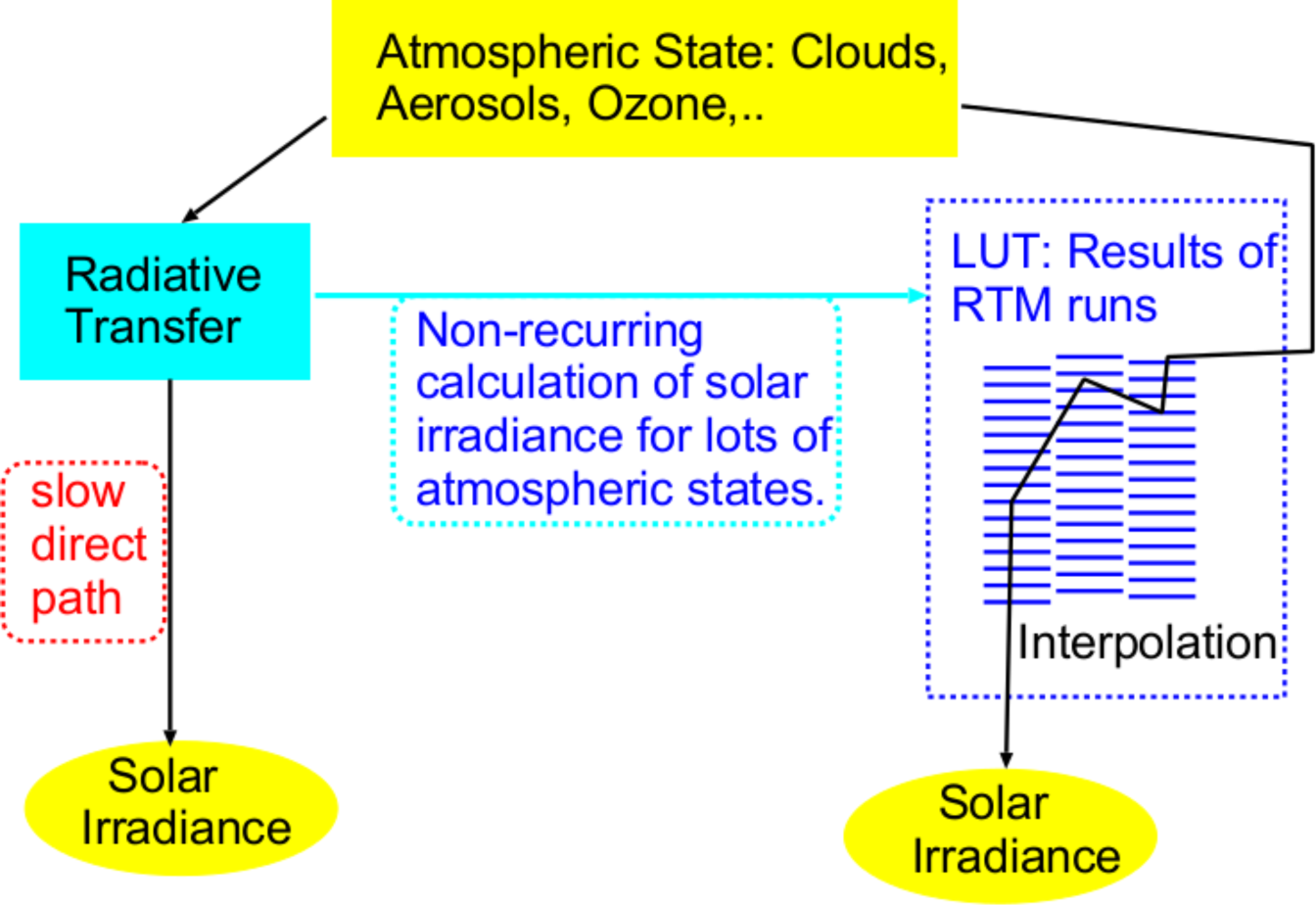
A look-up table (LUT) is a data structure used to replace a run-time calculation with a simpler interpolation operation within discrete pre-computed results, see Figure 1 as an illustration. The idea behind the LUT approach for irradiance retrieval is to achieve the same accuracy as with the direct usage of a RTM, but without the need to perform RTM calculations for each pixel and time. This results in a significantly improved computing performance.

Figure 1.
Illustration of the principle scheme of a LUT approach. The relation of the transmission to a variety of atmospheric states is pre-calculated with a radiative transfer model (RTM) and saved in a look-up table (LUT).
The analysis of the radiative processes in the atmosphere has been the basis for the development of the hybrid eigenvector LUT approach. The analysis of the system’s interaction allows the selection of processes, which have to be considered within a basis look-up table (LUT) from those processes that can be parameterized by simple equations and those that can be neglected.
The effect of aerosol scattering and absorption on spectrally resolved irradiance (denoted as Iλ) are considered within a 3-dimensional basis LUT. Iλ is calculated for different values of Aerosol Optical Depth (AOD), single scattering albedo (ssa) and asymmetry parameter (gg), and the results are saved in the LUT. The effect of ozone, water vapor or surface albedo on the solar surface radiation does predominantly not depend on any other atmospheric components including aerosols. Hence the basis LUT has been calculated for fixed values of ozone (335 DU), water vapor (15 mm) and surface albedo (0.2). The effect of variations in water vapor (H2O), ozone (O3) and surface albedo (SAL) is corrected after linear interpolation to the given aerosol state (defined by aod, ssa and gg) has taken place. Hence, the overall approach to calculate the clear sky surface irradiance in each wavelength bin λ, can be summarized as:
where, Iλ is the final spectrally resolved irradiance for cloud free skies in the respective wavelength bin λ.
is the spectrally resolved irradiance for a given aerosol state derived from the basis LUT for fixed water vapor, ozone and surface albedo.
and
are the corrections of deviations in water vapor and ozone, respectively, from the fixed values used in the LUT. Finally SALλ,cor is the scaling to the given surface albedo relative to 0.2, which has been used in all previous steps. Further, the Modified Lambert Beer function (MLB) [37] is used to reduce the needed calculation for the basis LUT. The modified Lambert Beer function extends the Lambert-Beer relation to broadband radiation and global irradiance. By application of this function the LUT entries only needs to be calculated for two solar zenith angles (SZA). The other SZAs are considered by application of the MLB function. Further details of the MLB function are discussed in [37], and, further details on the calculation of the basis LUT used to derive
are given in [24]. The direct irradiance is derived using the same approach (Equation (3)) but without the need for a surface albedo correction.
The basis LUT contains MLB parameters for 11 aod values (0, 0.1, 0.2, 0.3, 0.45, 0.6, 0.8, 1.0, 1.2, 1.5, 2.0) times three ssa values (0.7, 0.85, 1.0) times two gg values (0.6, 0.78). The spectral effect of aerosols is considered by application of a standard aerosol model [38,39].
For any given aerosol state the nearest neighbors are selected from the LUT and the solar irradiance is interpolated by distance weighting according to the given AOD, ssa and gg values. At this stage the solar surface irradiance is given for fixed water vapor, surface albedo and ozone values. In order to correct for deviations between the the fixed and the real values the parameterizations (Equation (3)) described in detail in [22,24] are applied as consecutive steps. To illustrate the correction an example is given for water vapor effect. The effect of deviations of H2O on the solar irradiance relatively to the fixed value is quantified by application of the following correction, which is equivalent to the respective broadband correction applied in [22]:
ΔIH2O,λ is the difference between the irradiance
for the real amount of water vapor and Ibasis,λ resulting from linear interpolation within the basis “aerosol” LUT. ΔIH2O,λ is calculated for the following set of input parameters (θz = 0, a rural aerosol type with aod = 0.2, ssa = 0.94, gg = 0.75, 345 DU ozone, and SALλ = 0.2). bλ is a “fitting” parameter applied to match the solar zenith angle dependency of water vapor absorption.
2.4. Spectral Correction of the Broadband Cloud Transmission
The Heliosat method provides the broadband effective cloud albedo (CAL) which is related to the cloud transmission, also referred to as clear sky index. In order to correct the spectral effect of clouds the broadband cloud transmission is transferred to the spectrally resolved cloud transmission by application of spectrally resolved conversion factors (Equation (7)).
The broad band cloud transmission corresponds to the clear sky index kbb defined as the ratio of solar surface irradiance I to clear sky irradiance Ics:
The clear sky index is related to CAL as given by the Heliosat relation (e.g., [32] or [36]) via:
Compared to the original equations the relation has been slightly modified. In the former version the clear sky radiation could reach 1.2 times the clear sky irradiance, here it is limited to 1.05 times.
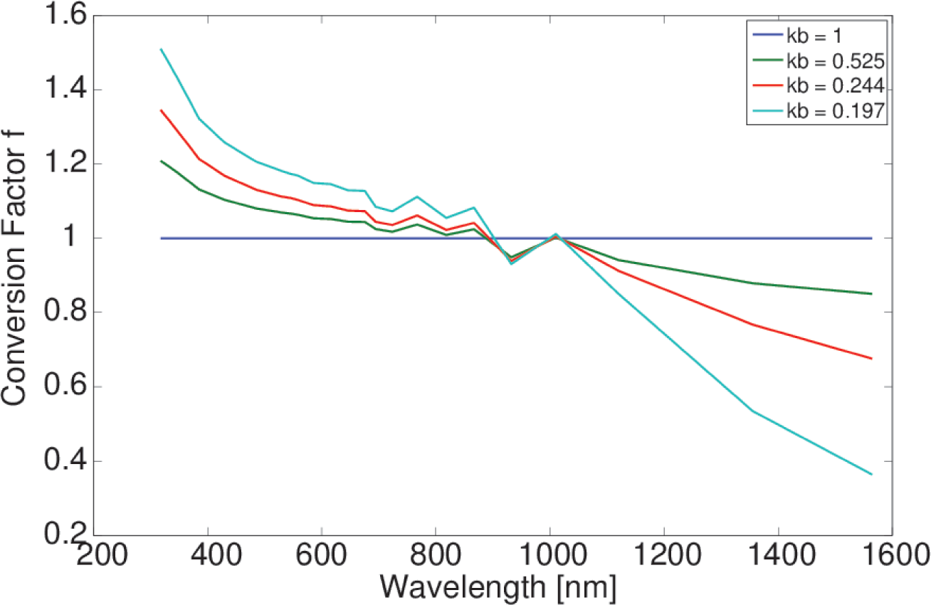
The presence of clouds results in a shift of clear sky spectrum from the red towards the blue range. Hence, a conversion from the broadband cloud transmission given by kbb to a wavelength dependent transmission kλ is required. This is done by the calculation of conversion factors. These conversion factors are calculated for each wavelength band using Equation (7) in order to consider the spectral effect of clouds on the broadband transmission.
here, fλ is the conversion factor,
and
are the clear sky indices for the wavelength bands (denoted by λ) and the broadband (denoted by bb), respectively, calculated with the radiative transfer model (denoted by RTM) libRadtran.
The RTM runs have been performed for the different wavelength bands and for the broadband with SAL and SZA set to zero and for cloud layers with cloud optical depth values of COD = 0, 10, 20, 40, 80 and 160. The corresponding clear sky indices
and
are gained through division of the resulting solar surface irradiance by the irradiance for COD = 0 for the respective spectral band. The resulting conversion factors are shown in Figure 2.
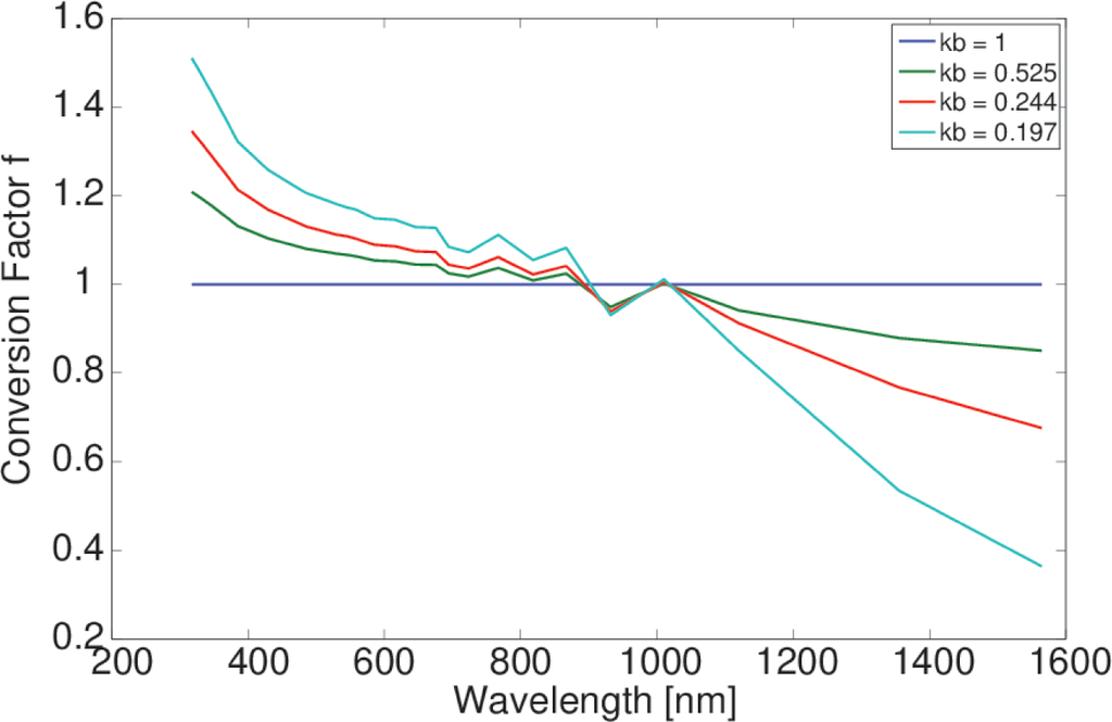
Figure 2.
Conversion from the broadband cloud transmission described by the clear sky index kbb to a wavelength dependent transmission
. The corresponding conversion factor f is given for different broadband clear sky indices kbb. This figure has been previously published in [24].
The conversion factors are saved in a LUT and applied to correct the wavelength effect of clouds on the clear sky index (see Equations (8) and (9)).
here, kλ is the derived spectrally resolved clear sky index and
is the broadband clear sky index derived from the satellite observations (CAL). Iλ is the spectrally resolved all sky and Ics,λ the spectrally resolved clear sky irradiance, respectively. Ics,λ is derived with the clear sky method described in Section 2.3. The broadband solar surface irradiance is given by the sum of the spectral bands.
2.5. Direct Irradiance
The direct irradiance SID is derived using Equation (10) [37]:
where k is the clear-sky index, SID is the all sky direct irradiance and SIDclear is the direct irradiance under clear skies, derived with SPECMAGIC using the equivalent approach than that discussed in Section 2.3. Equation (10) is an adaptation of the Skartveit diffuse model [40].
The Direct Normalized Irradiance (DNI) is derived by division of SID by the cosine of the solar zenith angle.
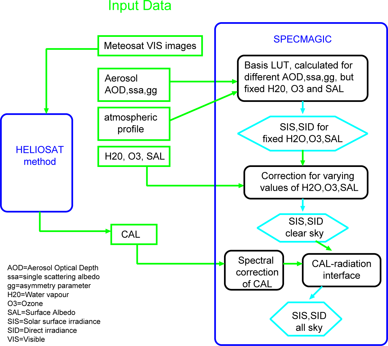
Figure 3 illustrates the interaction of Heliosat with SPECMAGIC and the relation to the respective calculation steps and input.

Figure 3.
Overview of the processing of the solar surface irradiance and used input. The input data is described in more detail in the next section.
2.6. Input on Atmospheric State
Spatial and temporal homogeneity (stability) is an essential requirement for proper climate trend analysis. Further, high accuracies are required for the monitoring of extremes and climate service applications (e.g., solar energy). The input data needed for the retrieval of solar surface radiation affects the accuracy as well as the homogeneity of a data set. Hence, selection and evaluation of input data is an crucial step for the retrieval of a climate data record and discussed in this section. Table 1 show an overview of the Input on Atmospheric State.

Table 1.
Overview of the atmospheric input used for the generation of SARAH.
2.6.1. Satellite Raw Images
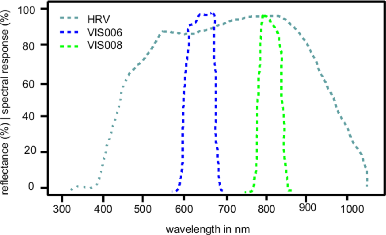
Satellite images are needed for the retrieval of the effective cloud albedo, which is in turn used for the estimation of the solar surface radiation, see Section 2.2. For Meteosat First Generation (MFG) satellite series (1983–2005) the broadband visible channel of the MVIRI instrument has been used. In detail, level 1.5 rectified image data of digital counts (not radiances) in openMTP data format. As a result of the self-calibration method applied within the retrieval of CAL [11] calibrated (inter-calibrated) radiances are not needed by the method. This approach follows the EUMETSAT recommendation given in [41], “it is necessary to rely to a great extent on vicarious, or external, calibration techniques in order to maintain product quality.” The spectral characteristics of the channels discussed hereafter are diagrammed in Figure 4. The SEVIRI instruments on-board the Meteosat Second Generation (MSG) satellites do not continue to provide the same spectral broadband information in the visible as the MVIRI instruments on-board of MFG for the full disk. The spectral characteristics of the discussed channels are shown in Figure 4. The use of one of the narrow-band VIS006 or VIS008 channels instead of a broadband channel leads to significant inhomogeneities in the data record, which is mainly due to the different spectral response [36].

Figure 4.
Overview of the spectral response of the MVIRI / SEVIRI channels, HRV stands for MVIRI broadband channel, VIS006 and VIS008 for SEVIRI spectral channels.
Hence, broadband observations are preferable for a consistent prolongation of the time series from the MVIRI instruments. A linear combination of the MSG/SEVIRI visible narrow-band channels (VIS006 and VIS008) provides a workaround as it simulates a broadband channel [42]. This approach has been shown to support a homogeneous retrieval of surface solar radiation between MFG and MSG [43]. Figure 4 provides the spectral response of the MVIRI broadband channel and the SEVIRI VIS006 and VIS008 channels. For consistency reasons CAL has been retrieved in 30 min resolution, which corresponds to the MVIRI temporal resolution. Further information on MSG and the SEVIRI instruments are given [1].
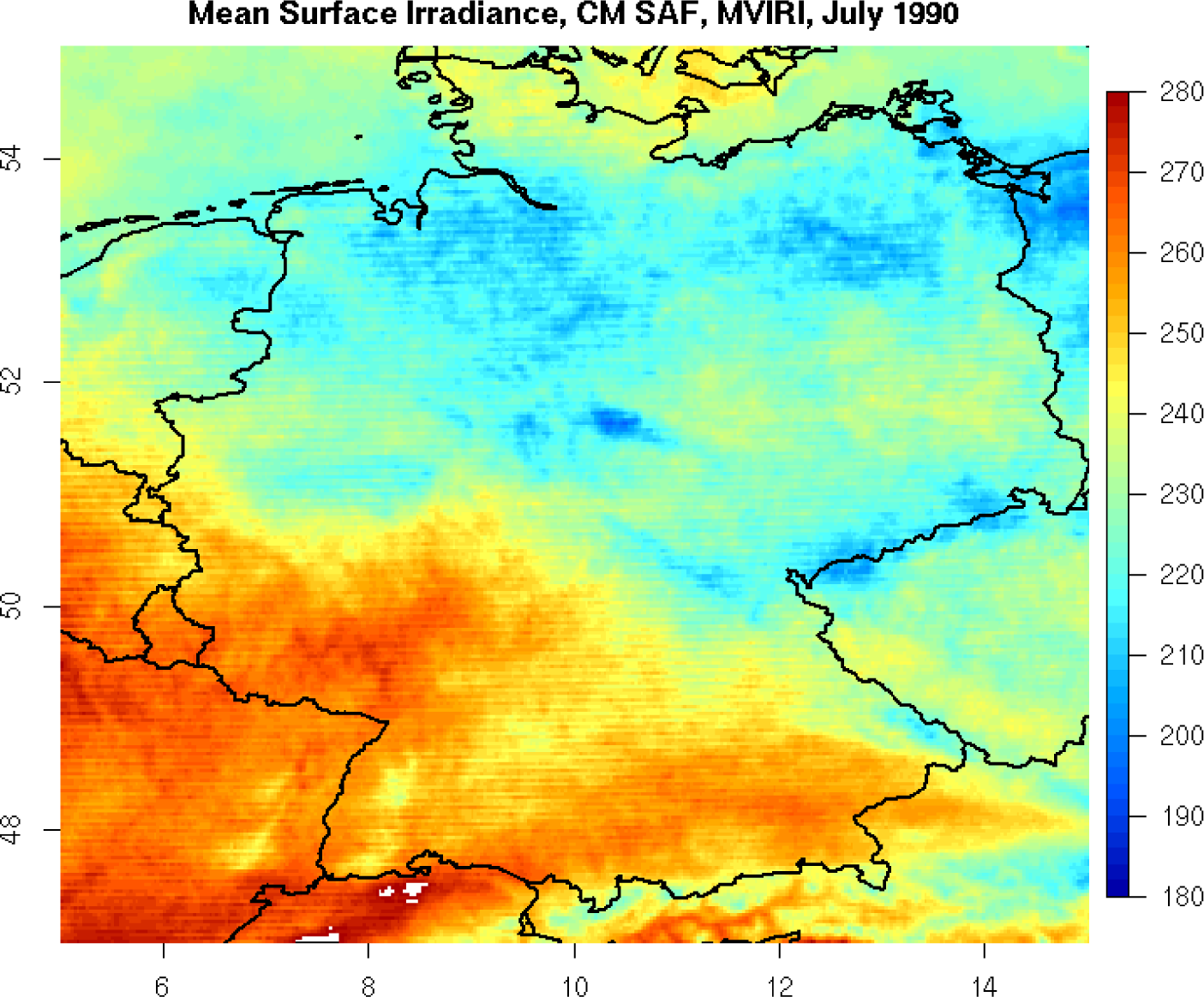
The previous MVIRI climate data record of CM-SAF [26] shows a good overall accuracy [25]. However, some artefacts have been found which are related to the raw image data. The MVIRI data set shows stripes in some daily means of the solar surface irradiance from 1983 to 1993, see Figure 5 for example. It has been found that these stripes go back to stripes in the MVIRI raw images, see Figure 6 for example.

Figure 5.
Example of stripes in the surface radiation products, here SIS daily mean.
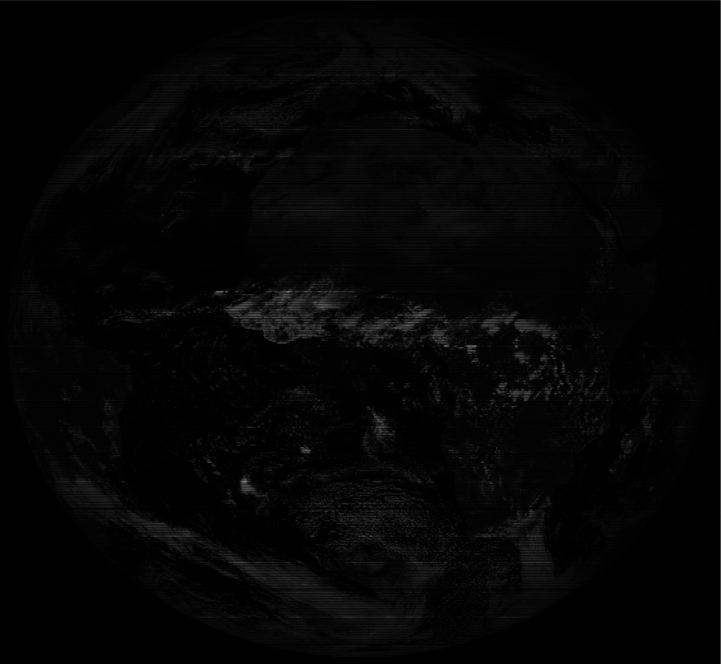
Figure 6.
Example of stripes in the MVIRI raw data. These stripes have been not corrected and led to the stripes in the radiation products illustrated in Figure 5.
Due to limitations of data transmission capacity only every second line of the broadband visible channel had been transmitted during night and twilight hours. This has been accounted for within the processing of the previous CM-SAF MVIRI only data record according to EUMETSATs information about the affected time slots. However, it has been fount that much more images are affected than it has been assumed within the MVIRI processing. For those images physically undefined lines have been erroneously interpreted as defined because the pixel values are technically within the allowed data range. This in turn is a result of missing no-data value in the raw images. The consideration of physically undefined lines led to stripes in CAL and subsequently in the radiation products as well (see CM-SAF service messages and Figure 5 for example). More over, in addition to the above discussed problem many other images are corrupted (e.g., incomplete images, detector failure in parts of the image) without being documented or listed as such prior to the generation of SARAH.
Thus, a visual inspection of the images has been performed for the period 1983 to 1994 in order to detect corrupt or incomplete images. This visual inspection has been very time consuming, but the only possibility to avoid the use of corrupt or incomplete images.
As the quality of the CAL retrieval relies on statistics it is desirable to have as much usable images as possible. Hence correction of the corrupted images has been performed as follows. The physically undefined lines have been filled by spatio-temporal interpolation using spatially adjacent lines of the same time slot as well as the respective lines from adjacent time slots. The adjacent time slots have been visually checked for completeness beforehand. As a consequence, no significant striping is apparent in the corrected images, see Figure 7 for example. Images with un-fixable bugs have been identified and have not been considered for the processing of the CDR in order to avoid its corruption. The evaluation of the raw data has been an essential step for the improvement of the solar surface radiation climate data records. The stripes of the solar surface radiation has been vanished after the correction, see Figure 8 for example.
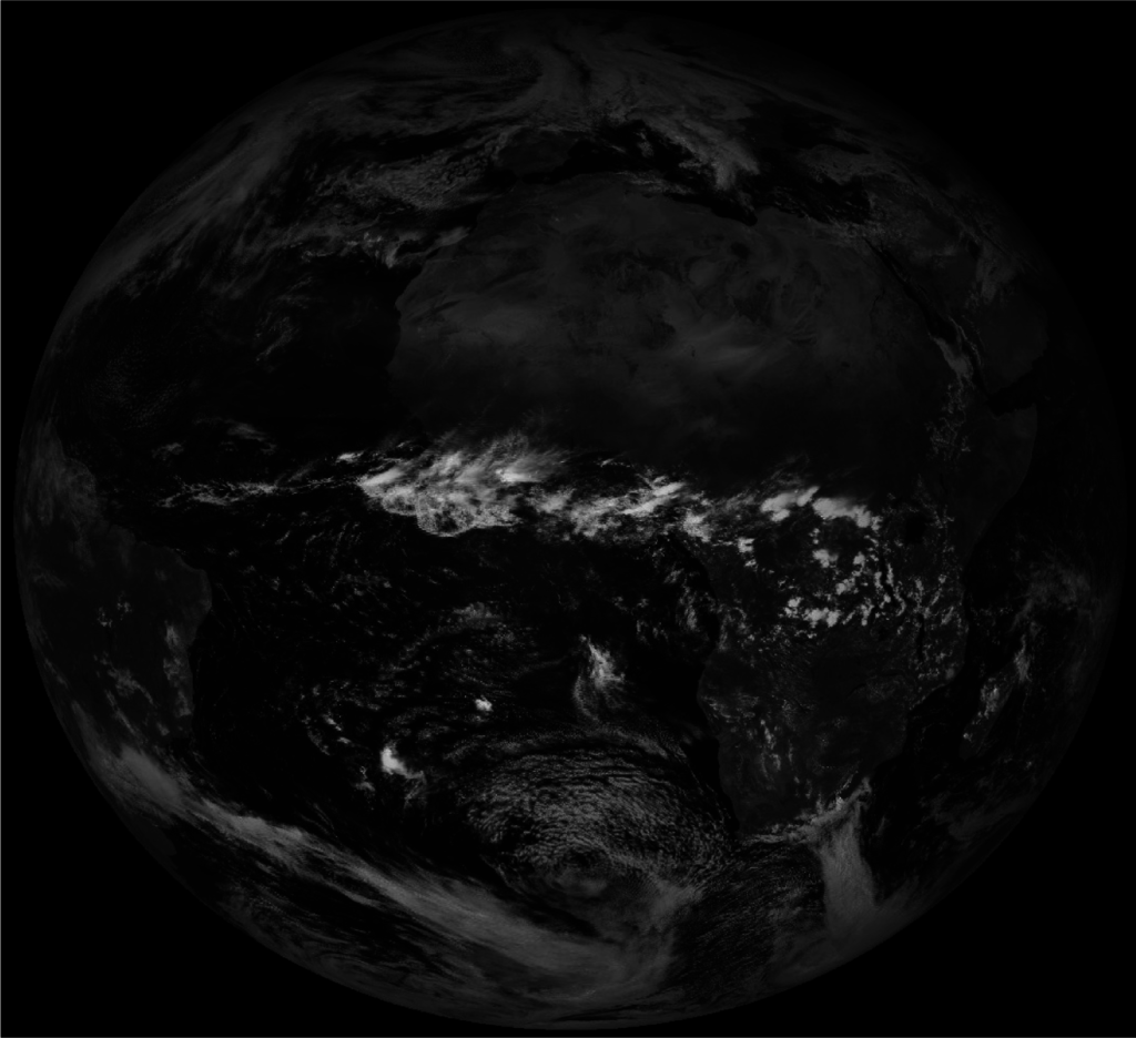
Figure 7.
Example of a corrected MVIRI raw data image.
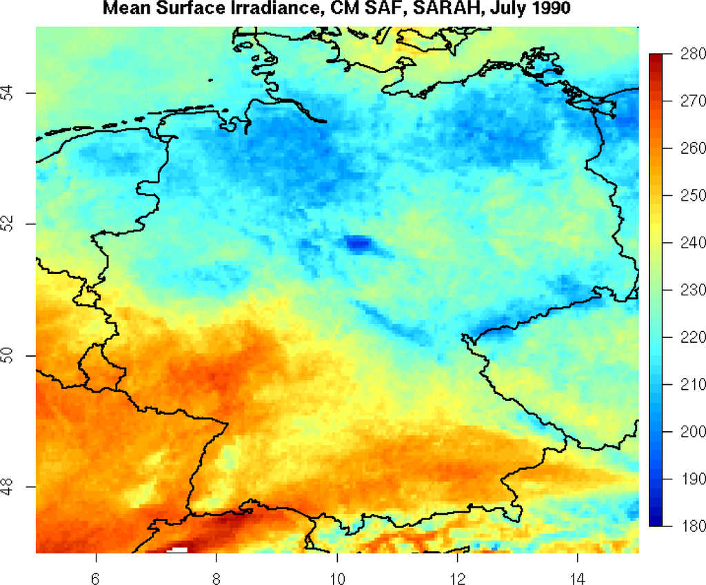
Figure 8.
Example of SIS image after the correction of the raw data. The stripes in the surface radiation products are not apparent any more.
The complete time series of the Meteosat satellites has been processed. The respective data covers the period 1983–2013. Table 2 provides a list of the used satellite data sets.
Table 2.
Major operational periods of the Meteosat satellites used for the generation of SARAH.
2.6.2. Aerosol
A monthly mean aerosol climatology has been generated by using the aerosol information provided by the European Centre for Medium Range Weather Forecast within the scope of the MACC project–Monitoring Atmospheric Composition and Climate. The MACC data results from a data assimilation system for global reactive gases, aerosols and greenhouse gases. It consists of a forward model for aerosol composition and dynamics [44] and an data assimilation procedure [45]. It has recently been used for the estimation of aerosol radiative forcing [46]. The MACC reanalysis data is generated on a Gaussian T159 grid which corresponds to ~ 120 km spatial resolution. For the use within CM-SAF it has been regridded to a 0.5 × 0.5 degree regular latitude-longitude grid.
MACC has been evaluated to perform significantly better than the “Kinne” [47] GADS/OPAC [48,49] and HAC-v1 climatology [50], see [51] for details.
However, in a further study [52] it has been evaluated that a modification of the MACC AOD leads to an even better performance. The modification has been performed as described in Equation (12).
Here, AODSARAH is the AOD used for the generation of the SARAH data set and AODMACC is the original MACC AOD. The final climatology consists of monthly long term means on 0.5 × 0.5 degree latitude-longitude grid. The respective AOD values are given for 550 nm. The pixel value is derived by spatial interpolation and assignment of the respective monthly mean.
Gueymard [53] and Nikitidou et al. [54] showed that the consideration of temporal variations of aerosols as well as trends are important for the accurate retrieval of solar surface radiation, in particular for direct irradiance. Within this scope the use of a monthly aerosol climatology is a drawback. However, aerosol events as desert storms and biomass burning lead temporarily to an increase in CAL, which might account partly for aerosol variations, please see [52] for further details.
2.6.3. Atmospheric Absorbers: Water Vapor and Ozone
Water vapor is an important atmospheric absorber, affecting solar surface radiation significantly. Integrated water vapor has been taken from from ERA-40 reanalysis [55,56] up to 1987 and from 1987 onwards from ERA-interim [57,58]. Monthly means, remapped to 0.25 × 0.25 degree latitude-longitude grid, has been used as input to SPECMAGIC. The pixel value is derived by spatial interpolation and assignment of the respective monthly mean.
Ozone is a strong absorber in the UV spectral range, but the absorption is quite weak within the broadband spectrum, hence not of high relevance for the estimation the estimation of the solar surface irradiance. Thus, for ozone the climatological values from the standard atmosphere are used [59]. Information about the other atmospheric gases (e.g., O2) and the total number density is taken from the US standard atmosphere [59].
2.6.4. Surface Albedo
For the surface albedo the spectral albedo functions of 20 land-use types originating from the NASA CERES/SARB Surface Properties Project [60,61], available at [62], has been used as basis. Each land use type comes with a spectral albedo curve covering 0.2 to 4.0 micrometers. In addition to these curves measured spectral curves provided by libRadtran have been used to account for the spectral albedo data as far as possible. Please see [24,33] for further details. The diurnal variation of the spectral surface albedo is determined as a function of solar zenith angle, as given by [63]. The scene dependent solar zenith adjustment factors needed for this function are also taken from the NASA CERES/SARB Surface Properties Project.
The land-use types are fixed throughout the year, hence seasonal variation of the surface albedo are not considered, but the surface albedo information is only used for the calculation of the clear sky irradiance. This induces uncertainties of about 1%–2% in regions with frequent variations of snow cover. Occasionally higher uncertainties might occur.
3. Validation of the SARAH CDRs
In this section the validation results are presented and discussed.
3.1. Reference Data for Validation
The validation of the new data sets for the surface incoming solar radiation (SIS) and the surface incoming direct solar radiation (SID,DNI) is primarily performed by comparison with high-quality ground based measurements from the Baseline Surface Radiation Network (BSRN) [64]. The BSRN stations used for the validation are listed in Table 3. They cover the period from 1992 onwards.
Table 3.
List of BSRN stations used for the validation.
Only those stations that have an overlap of at least 12 months with the satellite data were used. This leads to 15 stations, which are located mainly in the Northern hemisphere, but they cover the main climatic regions and a substantial part (1992–2013) of the satellite time period. The effective cloud albedo (CAL), as a pure satellite product, cannot be validated by comparison with ground based measurements directly. However, the accuracy of CAL can be estimated by error propagation from the accuracy of the surface radiation, see Section 3.6 for further details.
Furthermore, the discussion of the validation results accounts for the non-systematic error of the BSRN data of 5 W/m2 for measurements of solar surface irradiance (global irradiance) [64]. The BSRN data has been obtained from the BSRN archive at the Alfred Wegener Institute (AWI), Bremerhaven, Germany ( www.bsrn.awi.de). In a first step the BSRN data has been quality controlled using the tests proposed by [65]. To ensure a high quality of the reference data set, only those BSRN measurements that pass the limit tests are considered in the calculation of the daily and monthly averages. To derive monthly- and daily-averaged values from the surface measurements, the method M7 proposed by [66] was employed to reduce the impact of missing values. The uncertainty of the derived monthly means is on average ±8 W/m2 [28].
To assess the quality of the satellite data set with the BSRN surface observations, the difference in the spatial representativeness between these two observing systems needs also to be considered. Depending on the local spatial distribution of surface radiation the impact can be in the range of 4 W/m2 for monthly mean data [28] and even larger for daily mean surface radiation data. Due to its higher temporal and spatial variability it must be assumed that the level of uncertainty of the direct normal radiation (DNI) is larger than the level of uncertainty for solar surface irradiance (SIS). Further, circumsolar radiation contributes to the direct irradiance. This contributes to an enhanced uncertainty of DNI due to reasons related to different measurement geometries as well as differences relative to the definition of direct irradiance in RTM or solar energy applications, please see [67] for further details.
For a climate data record it is of interest to assess also the temporal stability with long-term reference measurements. BSRN measurements are not available before 1992, therefore data from the longer time series of the Global Energy and Balance Archive (GEBA) project has been used for this purpose. GEBA contains monthly mean surface irradiance data sets from ground observations including stations reporting prior to 1983 [68]. The temporal homogeneity of the GEBA stations has been evaluated by [69]. About 50 European stations have been found to be homogeneous over time. The data of these stations have been used to assess the temporal stability of the monthly mean SARAH SIS data set.
In addition to the validation with surface measurements, the quality of the CM-SAF SARAH data set is evaluated against the quality of the first release of the CM-SAF surface radiation data based on observation of the MVIRI instruments only, covering the period from 1983 to 2005 [25,36]. This data set is referred to as CM-SAF MVIRI data set throughout of the paper. It has been widely used and evaluated by numerous users over the last years. (e.g., [29,30,69–71]).
3.2. Statistical Measures
The validation employs several statistical measures and scores to evaluate the quality of the solar surface radiation data sets. Beside the commonly used bias and standard deviation, we also use the (mean) absolute difference (also referred to as Mean Absolute Bias) and the correlation of the anomalies derived from the surface measurements and the CM-SAF data set. For each data set we further provide the number of months that exceed the target accuracy to characterize the quality of the data sets.
In the following, the applied quality measures are described. The definitions of the statistical measures are taken from [72]. Thereby, the variable y describes the data set to be validated (e.g., SARAH) and o denotes the reference data set (i.e. BSRN). The individual time step is marked with k and n is the total number of time steps.
Bias: The bias (or mean error) is the mean difference between the two considered datasets. It indicates whether the data set on average over- or underestimates the reference data set.
Mean Absolute Bias (MAB): In contrast to the bias, the mean absolute bias (MAB) is the average of the absolute values of the differences between each member of the time series.
The MAB is also referred to as Mean Absolute Difference (MAD). The advantage of the MAB is that there is no cancellation of positive and negative (bias) values.
Standard deviation (SD): The standard deviation SD is a measure for the spread around the mean value of the distribution formed by the differences between the generated and the reference data set.
Anomaly correlation (AC): The anomaly correlation AC describes to which extend the anomalies of the two considered time series correspond to each other without the influence of a possibly existing bias. The correlation of anomalies retrieved from satellite data and derived from surface measurements allows the estimation of the potential to determine anomalies from satellite observations.
Here, for each station the mean annual cycle were derived separately from the satellite and surface data, respectively. The monthly/daily anomalies were then calculated using the corresponding mean annual cycle as the reference.
Fraction of time steps above the validation threshold (Frac): A measure for the uncertainty of the derived data set is the fraction of the time steps that are outside the requested thresholds Th.
3.3. Validation Results—Comparison Method
The daily and monthly means of the SARAH data set are compared with the respective daily and monthly means derived from the BSRN measurements. The means of the BSRN station have been derived independently using the complete temporal resolution (minutes) of the BSRN measurements. The comparison results in a mean bias, mean absolute difference, anomaly correlation, standard deviation and fraction of months above a given limit for each individual station and for all stations together.
Daily and monthly mean of DNI are calculated by an arithmetic average. SIS and SID data are averaged by application of an equation by Diekmann [73], which is preferable because of the large dependency on the solar zenith angle of SIS and SID, which makes the arithmetic averaging very sensitive to data gaps.
3.4. Validation Results—SIS
In this section the validation results of the Surface Incoming Solar Radiation, SIS are presented and discussed. The results of the validation of the monthly mean SARAH SIS data set are summarized in Table 4. The bias and the MAB are with values of 1.27 and 5.46 W/m2 remarkably low. In total about 94% of the monthly mean values show an accuracy better than 10 W/m2, by consideration of an uncertainty of the surface measurement of 5 W/m2 [64]. The results show that the accuracy is close to that of the ground measurements. The data set is also able to reproduce the anomalies of SIS quite well, which is documented by the high correlation of the monthly SARAH SIS anomalies (0.92) with the ground measurements. Also included in Table 4 are the corresponding statistical error measures of the CM-SAF MVIRI surface radiation data set [36]. It is clear that the quality of the new CM-SAF data set SARAH is substantially improved compared to the previously released CM-SAF MVIRI data set.
Table 4.
Results of the comparison between the monthly mean surface solar irradiance derived from BSRN measurements and the two CM-SAF surface radiation data sets.
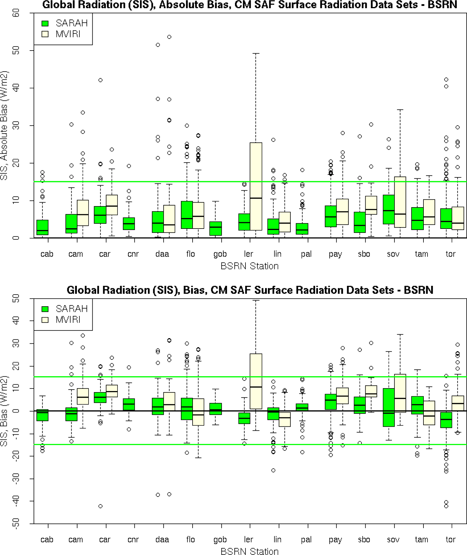
An illustration of the bias and the MAB at each BSRN station is shown in Figure 9. The box-whisker plots represent the range between the 25 and 75 percentiles (1st and 3rd quartile) by the colored boxes; the whiskers extend to 1.5 times the inter-quantile range or the maximum value, whichever is smaller. As already shown in Table 4, the new SARAH surface radiation data set has a substantially reduced bias and a lower MAB compared to the MVIRI CM-SAF surface radiation data set at each BSRN station. Particular improvements can be found at the BSRN stations Lerwick (ler), Carpentras (car), and Sede Boquer (sbo).

Figure 9.
Mean Absolute Bias (top) and bias (bottom) in W/m2 of the SARAH monthly mean solar surface irradiance.
3.4.1. Daily Means
Table 5 provides the validation result for the daily means of the new SARAH SIS data set and the previous CM-SAF MVIRI climate data record. As expected, the mean bias is almost identical to the value for the monthly means while the mean absolute bias for the daily means are about twice as high compared to those for the monthly means. However, an increase of MAB values has to be expected as a result of an decreasing averaging period, due to the fact that satellite data are compared to ground measurements. The basis for the comparison are half hourly means of satellite data representing a 3 × 5 km area with BSRN data representing point measurements. This reduces the comparability and increases the deviation between the data, e.g., MAB, for short averaging periods. Still, the mean absolute bias of 12.1 W/m2 between daily mean SARAH SIS and BSRN is remarkable low. Further, nearly 90% of the daily means show better accuracy than 15 W/m2. As for the monthly mean validation, the SARAH SIS data set shows improved performance for each quality measure compared to the CM-SAF MVIRI SIS data set.
Table 5.
Results of the comparison between the daily mean surface solar irradiance derived from BSRN measurements and the two CM-SAF surface radiation data sets.
The bias and the MAB of the SIS daily mean from the SARAH data set for the individual BSRN stations are shown in Figure 10.
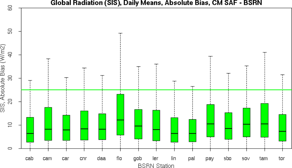
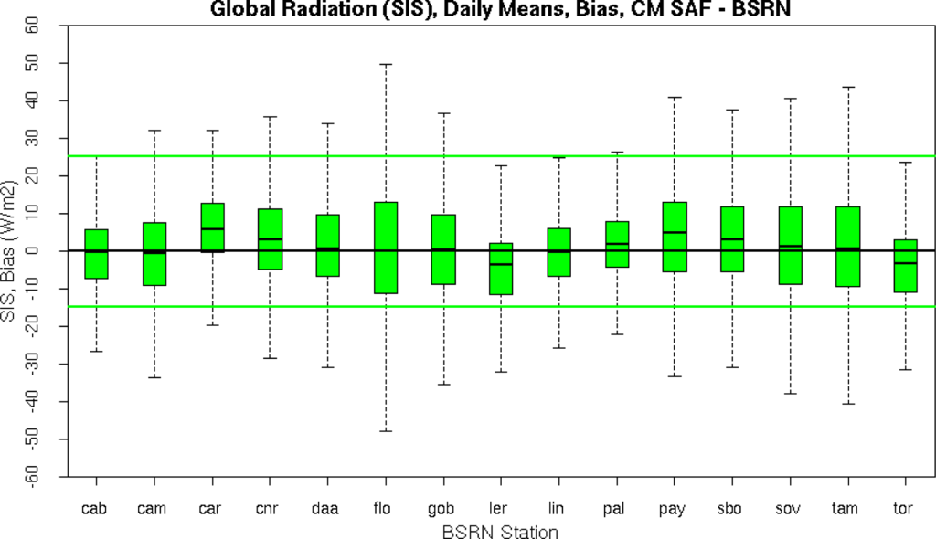
Figure 10.
Mean Absolute Bias and (top) and Bias (bottom) in W/m2 of the SARAH daily mean solar surface irradiance.
3.5. Validation Results: SID and DNI
This section presents the validation results of the SARAH direct radiation data sets (SID and DNI) compared to the BSRN surface reference observations. DNI is derived by division of SID with the solar zenith angle (SZA), see Equation (11). This means that the physics (retrieval method) applied to derive SID and DNI are identical. Table 6 shows the results of the validation of the surface direct radiation (SID) for the recent SARAH and the previous CM-SAF MVIRI data sets. The bias and the mean absolute bias are with 0.89 W/m2 and 8.2 W/m2 remarkably low for SID, showing the high accuracy of the data set. The MAB is thereby significantly lower than for the MVIRI data set. The substantial improvement of SARAH SID relative to MVIRI SID is also apparent in the other validation measures.
Table 6.
Results of the comparison between the monthly mean surface direct irradiance (SID) derived from BSRN ground measurements and the two CM-SAF SID data sets (MVIRI, SARAH). Further, results of the comparison between the monthly mean Direct Normal Irradiance (DNI) derived from BSRN ground measurements and the SARAH DNI data set.
For the solar energy community the direct normal irradiance is of high interest. Hence, the new SARAH data set offers the direct normal irradiance in addition to SIS and SID. DNI is not available from the older CM-SAF MVIRI data set. A small bias of 3.2 W/m2 is found in the SARAH DNI data set. The mean absolute bias is 17.5 W/m2. Considering the uncertainty of the surface measurement of about 10 W/m2, it can be expected that the accuracy of DNI is of about 10 W/m2, which is remarkably good. The standard deviation and, thus, the spread is slightly larger for DNI than for SIS (22.9 W/m2 compared to 11.6 W/m2), which results simply from the fact that DNI exhibits on average higher values than SID, due to the normalization with the cosine of solar zenith angle. This explains also that DNI shows larger values for Fracmon. The anomaly correlation shows a value of 0.87 and is almost identical to the respective SARAH SID value.
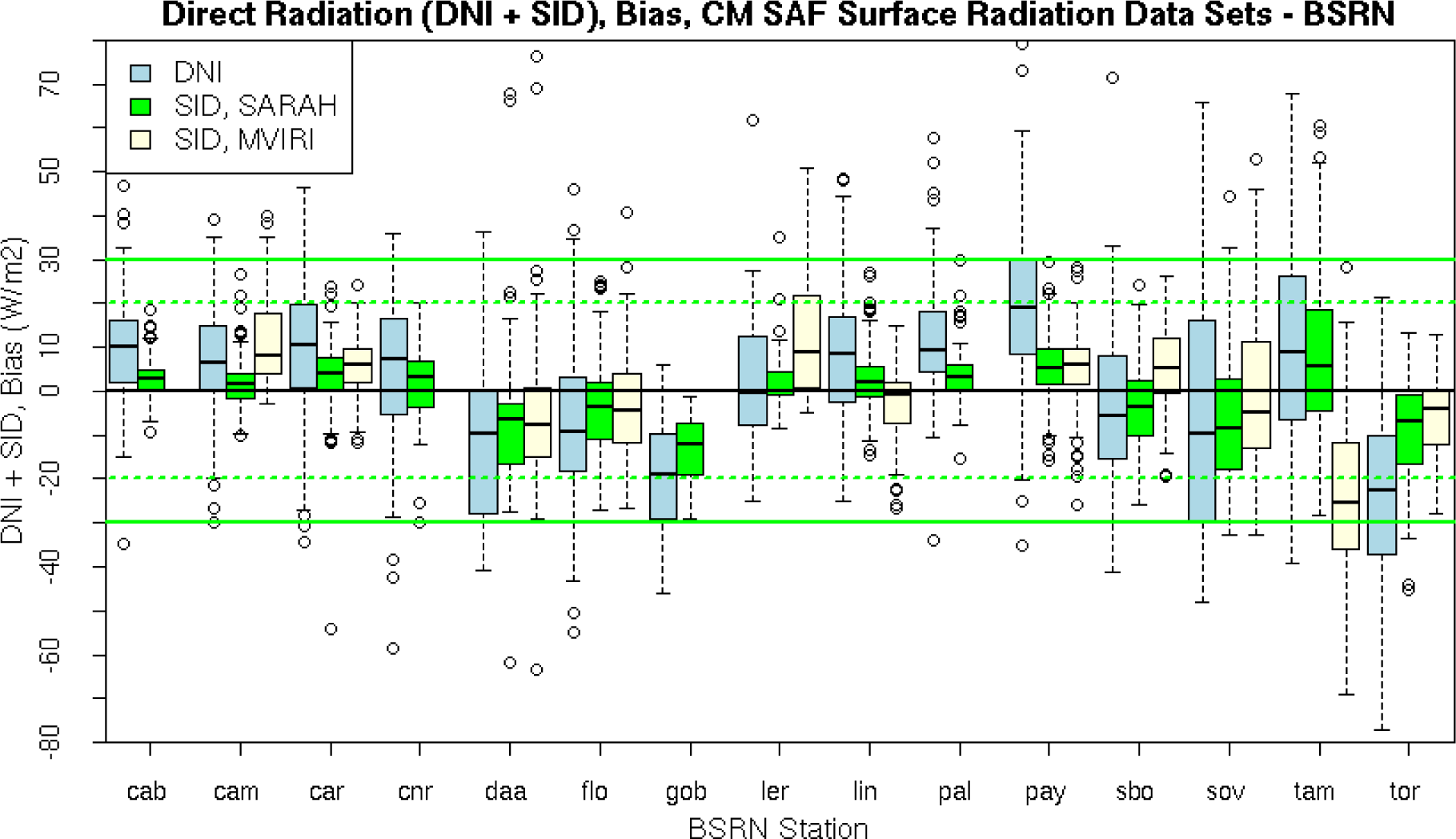
The results for the individual BSRN stations are shown in Figure 11. Beside the SID results (SARAH and MVIRI) the figure shows also the absolute bias of the monthly means of DNI and of SID from SARAH for each station. For most stations, the accuracy of SID from SARAH has improved compared to the previous CM-SAF MVIRI data set.
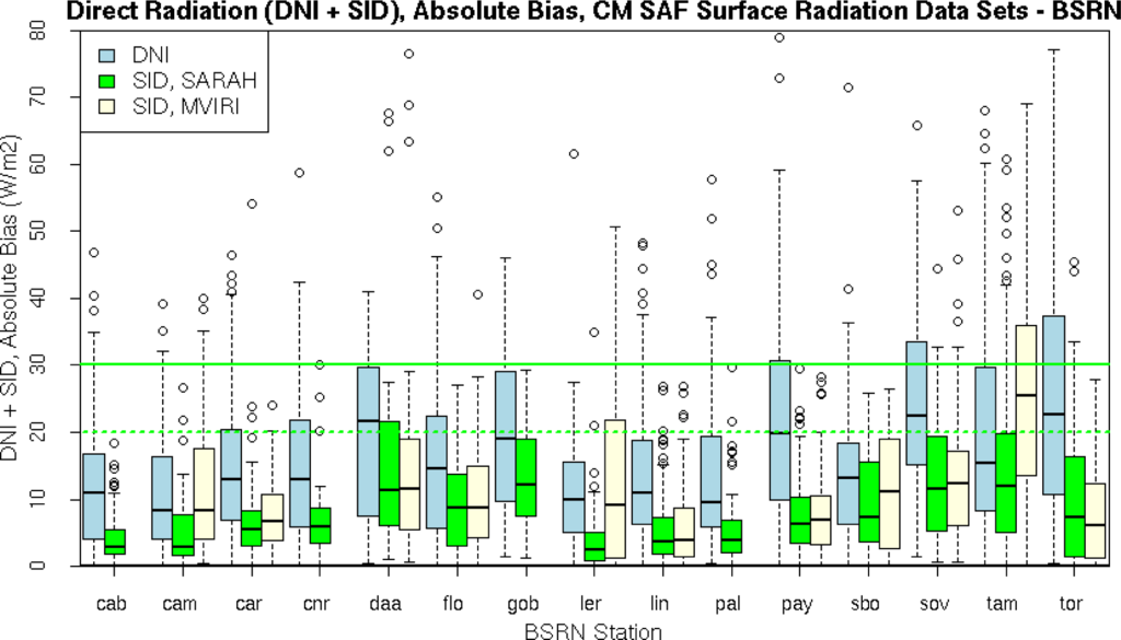
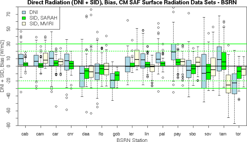
Figure 11.
Mean Absolute Bias and (top) and Bias (bottom) in W/m2 of the SARAH monthly mean solar surface radiation (SID,DNI).
Notably is the large negative offset in Toravere of about of about −27 W/m2 (Figure 11 bottom), which corresponds to a negative offset in SID of about 10 W/m2.
A reason for the relative large offset in Toravere could be an overestimation of clouds induces by the slant viewing geometry. For the same cloud scene the effective cloud albedo increases significantly for slant geometries as the effective cross section of the clouds observed from satellite increases. Further, for SID and DNI higher uncertainties are also expected in regions with high temporal and spatial variability in aerosol properties.
3.5.1. Daily Means
The validation results for the daily means of the CM-SAF SARAH direct irradiance data are shown in Table 7. The evaluation results for the surface direct irradiance (SID) shows also the aforementioned substantially improved performance of SARAH compared to the CM-SAF MVIRI data set. With exception of the bias these improvements are apparent in all error measures.
Table 7.
Results of the comparison between the daily mean surface direct irradiance (SID) derived from BSRN ground measurements and the two CM-SAF SID data sets (MVIRI, SARAH). Further, results of the comparison between the daily mean Direct Normal Irradiance (DNI) derived from BSRN ground measurements and the SARAH DNI data set.
For DNI the mean absolute bias is significantly larger than for the daily mean SID data set (34.4 W/m2 compared to 17.9 W/m2. However, this is a result of the overall higher values of DNI compared to SID. As for SID the daily mean DNI shows a larger spread than the corresponding monthly means.
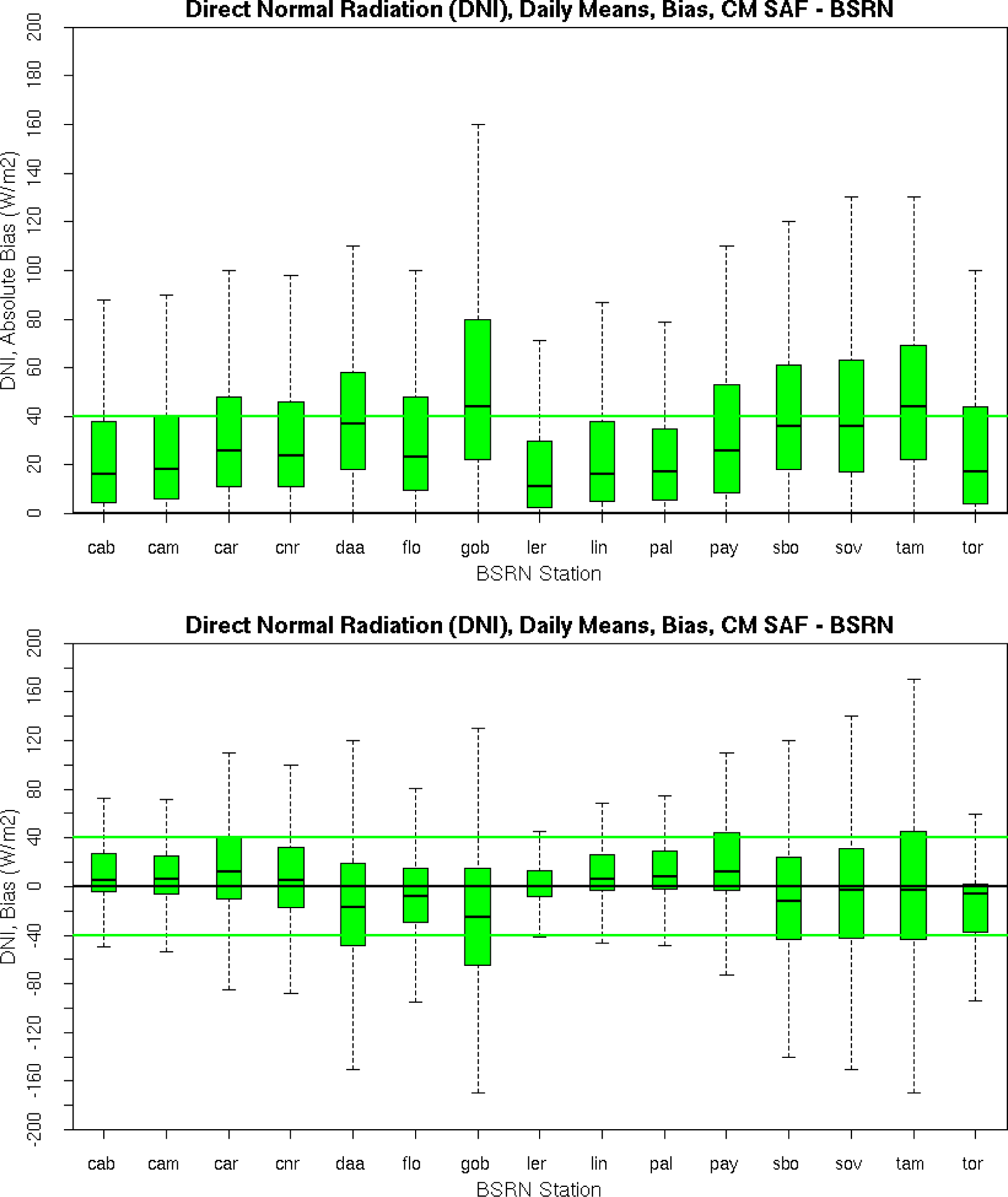
The results for the individual stations are shown in Figure 12.

Figure 12.
Mean Absolute Bias and (top) and bias (bottom) in W/m2 of the SARAH daily mean direct normal irradiance–DNI.
The daily means show the same features as the monthly mean direct radiation products. Relatively large mean absolute bias values are found at the predominantly sunny, cloud free (desert) stations of Gobabeb, Sede Boqer, Solar Village and Tamanrasset.
3.6. Validation Results: CAL
CAL is only observable from space. Thus, it can not be validated with ground based reference data sets. However, its accuracy can be estimated by error propagation using the relation between SIS and CAL. The relation between the effective cloud albedo CAL and the solar irradiance is essentially given by:
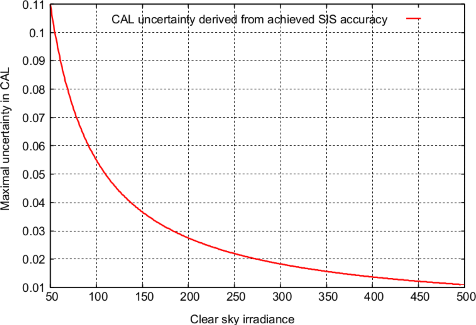
Uncertainties in SIS are due to uncertainties in the effective cloud albedo and due to uncertainties in the clear sky irradiance. Here we assume a perfect clear sky irradiance (no errors), which relates all uncertainties in SIS to the effective cloud albedo and provides thus a worst case scenario for the CAL accuracy. The clear sky irradiance is, of course, not error free, hence the CAL errors are lower than the estimated values. Thus, based on Equation (18) the “worst case” accuracy of the effective cloud albedo can be derived as a function of the clear sky irradiance. Figure 13 shows the maximal error in the cloud index, which would only be given for a mean absolute bias of zero in the clear sky irradiance. It is clear that this evaluation method is a workaround, but as aforementioned the effective cloud albedo is a satellite observable, and can thus not be “validated” with ground based reference data. However, as a result of the low error in SIS it can be expected that the uncertainty in CAL is usually significantly below of 0.1, with exception of bright surfaces (desert, snow) and slant viewing geometries where higher errors have to be expected. Higher uncertainties in CAL affects also SIS, SID and DNI.
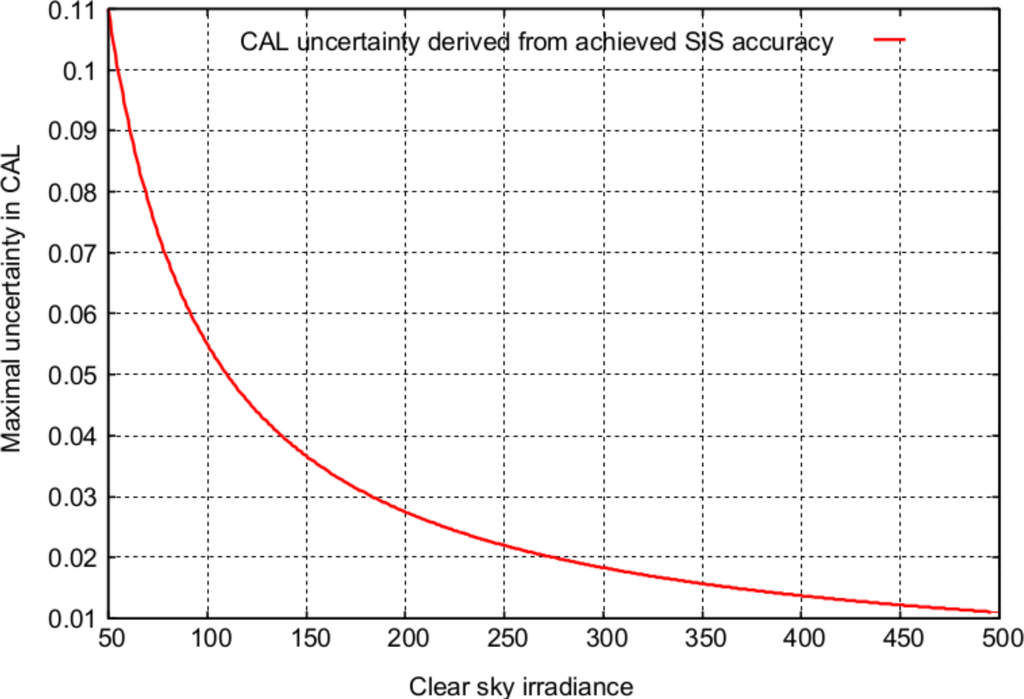
Figure 13.
Maximal uncertainty of the monthly mean cloud albedo in dependency of the clear sky irradiance. The estimation of the CAL uncertainty is derived by error propagation based on Equation 18. It depends therefore on the clear sky solar surface irradiance.
3.7. Homogeneity/Stability of CDRs
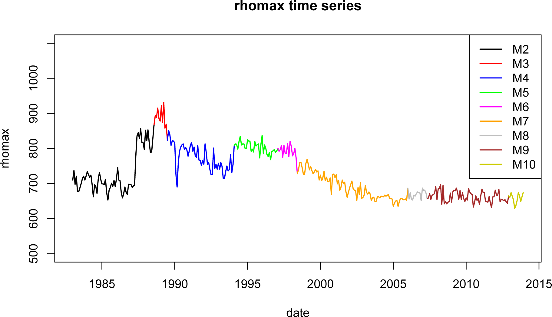
High accuracy (Bias, MAB) and precision (SD, Fracmon) are the main quality measures for monitoring of climate extremes and solar energy applications. However, for trend analysis the temporal homogeneity of the data record is of significant concern. “Calibration” and inter-calibration of satellite instruments are an essential pre-requisite for homogeneous and stable time series. Please see [51,74,75] and references therein for further details. Hereafter, some specific “calibration” issues are briefly discussed in order to enable a better understanding, without aiming for a detailed scientific discussion. The visible channels of the MVIRI and SEVIRI instruments are calibrated before the launch of the satellites. However, these instruments are not equipped with an on-board calibration units in the visible channels. The sensitivity of the satellite instruments degrades seriously over time in the visible due to ageing processes of the optical devices. See Figure 14 for example and [74] for further details. The degradation of the sensitivity could easily lead to artificial trends in the retrieved solar radiation products. In addition, newly launched instruments of the same series (e.g., MFG series) are not degraded and show therefore a different sensitivity, which could easily lead to jumps in the time series of the observed reflection. However, the mentioned issues can be resolved by vicarious calibration. With this method gauge adjustment (inter-calibration) of the instruments is performed by comparison of reflectances for “stable” targets (e.g., desert & cloud targets). A vicarious calibration is applied by Eumetsat [75] for SEVIRI onboard of MSG (starting with Meteosat-8), but has been not performed during the operation of the MVIRI instruments. Here, only a smooth transition between Meteosat-5 -6 and -7 has been generated by intercomparison and adjustment of the observed reflectances, which does not resolve the degradation issues. Further, the failure of the broadband visible channel on SEVIRI (High Resolution Visible, HRV) inhibits the prolongation of the time series with an input signal with comparable spectral response to that used for MVIRI [36]. The different spectral response of the visible channels induces serious inhomogeneities in CAL and the solar surface irradiance [36].

Figure 14.
Observed maximal reflection in the cloud target region. The degradation of Meteosat-6 to seven, as well as changes in the gauge, e.g., Meteosat-2, are clearly visible.
Summarizing, the change of satellite instruments of one series as well as the update to a new generation of satellite instruments can induce inhomogeneities in the retrieved effective cloud albedo and thus the solar surface irradiance. The generation of a homogeneous climate data record from satellite images in the visible is a quite challenging task. This might be one reason for the minor role of remote sensing data in climate trend analysis, although that satellites are the only observational source of information over the oceans and many other regions of the world. Thus, analysis of the homogeneity of SARAH is an important issue.
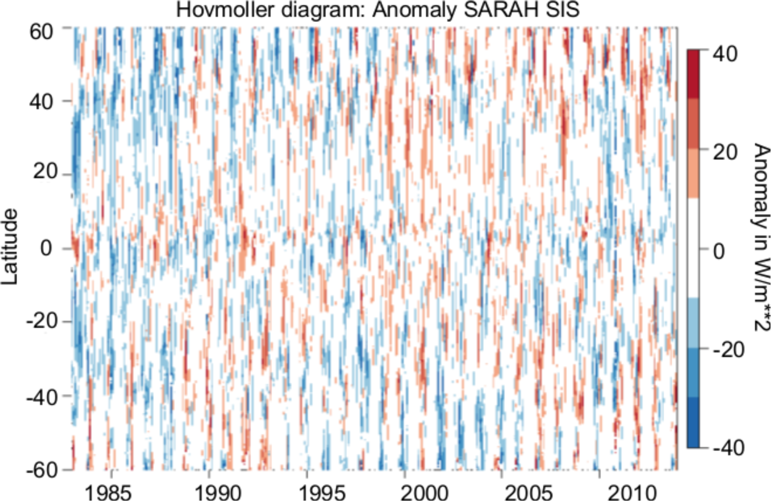
A common method to assess the homogeneity of a climate data set is to analyze the anomaly time series for any obvious jumps. Changes in the mean state from one satellite to the other would be apparent as an increase or decrease in positive or negative anomalies. Figure 15 shows the Hovmoeller diagram of the monthly mean anomalies of SIS and DNI. The time covers the full period of the SARAH data set starting with Meteosat 2 in 1983 until Meteosat 10 in 2013. No obvious artificial jumps or trends are apparent in the time series of the anomaly for the whole time period, indicating a good homogeneity of the SARAH data set.

Figure 15.
Hovmoller diagrams of the monthly mean anomaly of SIS. and (bottom) DNI.
To evaluate and quantify the stability of the SARAH data set in more detail, references measurements from the GEBA data base are used in addition to BSRN. While the BSRN observations follow a high quality standard and are considered as a GCOS reference observing network, the data in the GEBA data base have a longer temporal coverage, which is important for the assessment of the temporal stability. To assess the temporal stability of the satellite-based data, the reference observations need to be stable over time as well. Selected European GEBA stations have been assessed with respect to their temporal stability and adjusted to ensure their homogeneity [69], only these stations are considered here.
Figure 16 shows the temporal evolution of the average bias between the monthly mean SARAH SIS data set and the measurements from the GEBA stations. Only stations with more than 95% available monthly means between 1983 and 2011 are considered to avoid artificial shifts in the mean time series due to changes in data availability. An optimal stability and match with the ground based stations would mean that no significant gradient in the linear regression is apparent. Any significant gradient indicates a mismatch between the trends of satellite and ground based data.
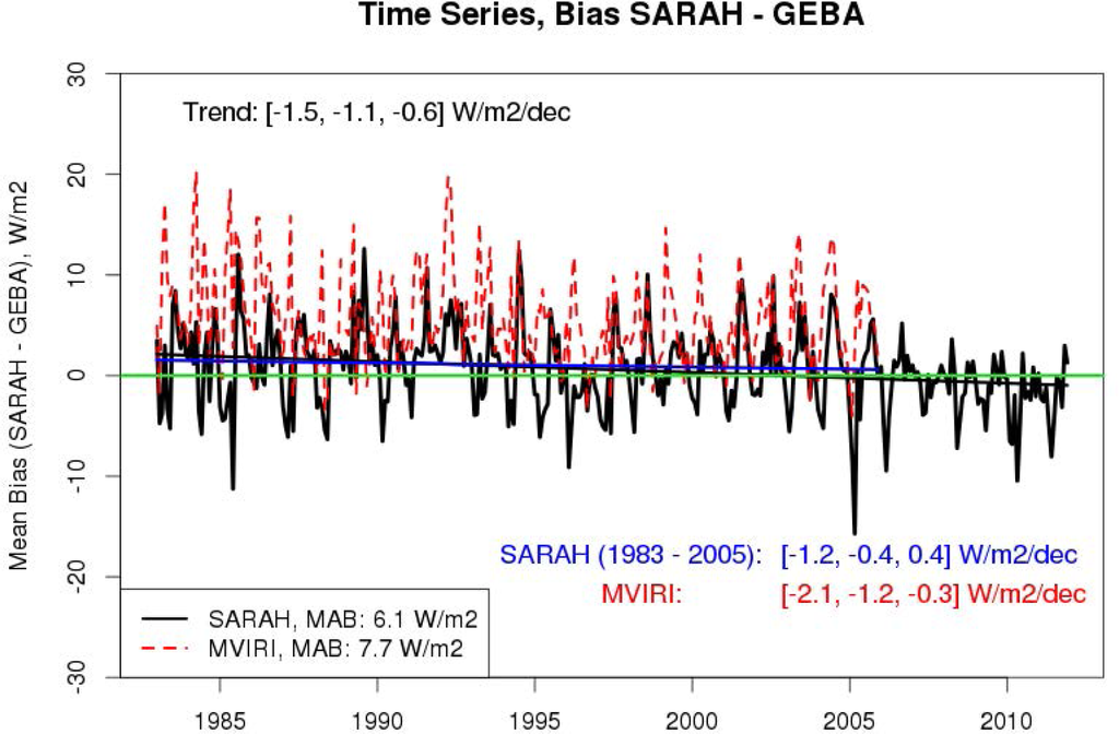
Figure 16.
Temporal evolution of the normalized differences between the CM-SAF data set and the GEBA data. The green line represents the zero line, the black and the blue straight lines represent the linear regression of the time series for the time periods 1983 to 2011 and 1983 to 2005 (both for SARAH), respectively. A gradient of zero in the linear regression would mean a perfect match between trends in the satellite and ground based data. Also given in the legend is the result of the analysis for MVIRI. However, the MVIRI trend is not diagrammed.
A negative decadal gradient of the bias of −1.1 W/m2/decade is detected between satellite and ground based data. This gradient is found to be statistically significant, but is rather small and might be in the range of the uncertainty of the ground measurements. This means that for trend analysis of the SARAH data set an uncertainty of about 1 W/m2/decade can be assumed for the time period 1983–2013.
Figure 16 shows also the corresponding trend analysis for the time period 1983–2005 for the SARAH and the CM-SAF MVIRI solar surface radiation. (Note that the MVIRI trend is not diagrammed, but only the numbers are given in the figure). While the bias of the MVIRI data set exhibits a significant negative trend of −1.2 W/m2/dec compared to the GEBA surface observations the SARAH SIS data set does not show a significant trend for the period 1983–2005. This is a remarkable improvement and demonstrates the enhanced stability of the SARAH data set compared to the previous CM-SAF MVIRI surface radiation data set. It is likely that the efforts concerning the raw data (Section 2.6) has been significantly contributed to this result. However, the differences in the SARAH trends for the period 1983–2005 relative to 1983–2013 indicates a serious break induced by the transition from MFG to MSG, which is also visible in the development of the bias over time, see Figure 16. It is likely that this break is resulting from a sub-optimal generation of the artificial HRV channel. It is evident that an adjustment of the channel combination is needed.
Nevertheless, overall the homogeneity of SARAH is remarkably high, in particular when considering that ground measurements are not a-priory homogeneous but require homogenization tests as well. In this respect the SARAH data set is an important key for the supplementation of climate trend analysis based on ground based measurements, in particular as many regions are not covered by well maintained ground based measurements.
Remote sensing based radiation products are the only observational sources that can provide trends of surface radiation with high spatial resolution and large geographical coverage. Figure 17 shows the trend for the full disk. It is evident that in many regions the trend is much higher than the expected uncertainty of 1 W/m2/dec. The large spatial structures in the trends demonstrate the importance of remote sensing radiation data for climate trend analysis. The large negative trends in the ITC region might indicate an enforcement and some latitudinal spreading of the Hadley circulation. This might be one driver for the positive trends in the sub-tropics and Central Europe. The significant negative trend close to the Antarctic might be one reason for the increase of the ice sheet there. Further trends and their analysis will be discussed in a forthcoming paper.
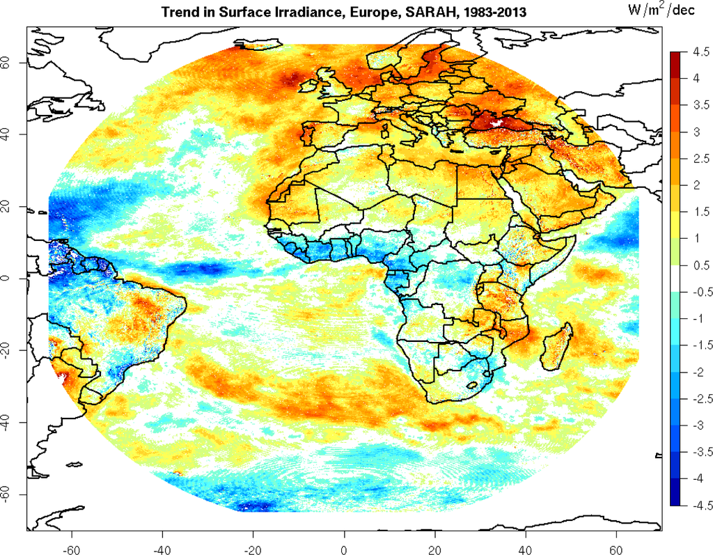
Figure 17.
Trend in the SARAH solar surface irradiance for the time periods 1983 to 2013.
4. Conclusions
The CM-SAF SARAH data set and its retrieval method has been presented and discussed. It is the first time that the SPECMAGIC [24] eigenvector-hybrid LUT approach has been exploited for the retrieval of a CDR of broadband solar surface irradiance.
The satellite-derived SARAH climate data records of the surface incoming solar and direct normal radiation (SIS and DNI) have been validated by comparison with observations from 15 high quality ground-based stations of the BSRN network. For the solar surface irradiance (SIS) the bias of 1.3 W/m2 and mean absolute bias of 5.5 W/m2 are close to the uncertainty of the ground based measurements for monthly means, and hence, close to the optimal accuracy of 3–5 W/m2. For SID, the bias and MAB are with 1 and 8 W/m2 remarkably good (3.1 and 17.5 W/m2 for DNI, respectively). By consideration of the uncertainty of the ground based measurements it can be assumed that the accuracy is better than 8 W/m2 for SID and better than 12 W/m2 for DNI. However, for both SID and DNI there is room and need for improvement of the accuracy.
The anomaly correlation show for all products very high values of about 0.9. The fraction of monthly values that meets high accuracies is around 85%–95%. Thus, SARAH radiation products are well suited for climate monitoring and analysis of extremes.
Prior to 1992 no BSRN measurements are available, hence the data set could not be validated with BSRN ground based measurements for the period 1983–1992. However, there is no physical reason why the accuracy of the climate data set should be significantly lower for this period. This argument is “proven” by comparison with GEBA measurements.
The evaluation of the CM-SAF SARAH solar surface irradiance with the old CM-SAF MVIRI surface radiation data set shows that the monthly and daily mean SARAH data have a higher quality than the previous CM-SAF MVIRI surface radiation data set.
Visual inspection and correction of the MVIRI raw data base has been performed. It is likely that this, together with an improved retrieval procedure have significantly contributed to the good SARAH validation results.
Special care has been taken to improve the homogeneity of the CDR. The stability of the SARAH SIS data set has been validated against European surface measurements (GEBA). A statistically significant negative trend in the bias of −1.1 W/m2/dec was found between SARAH and ground based measurements for the period 1983–2013. It can be assumed that trend analysis based on SARAH has an uncertainty of about 1 W/m2/dec. However, for the period covered by the CM-SAF MVIRI data set (1983–2005) no significant trend in the bias has been found in the SARAH data set. In contrast, the CM-SAF MVIRI data set shows a significant trend in the bias of −1.2 W/m2/dec for the same period (1983–2005). This demonstrates that the homogeneity of SARAH has significantly improved compared to the CM-SAF MVIRI data set. Further, it clearly indicates that the transition from MVIRI to SEVIRI induces a slight inhomogeneity in the SARAH data set. Nevertheless, overall, it is shown that the SARAH data set can be expected to be well suited for climate trend analysis.
The uncertainty of the effective cloud albedo is in general better than 10%. The validation results show that the SARAH radiation records are in general well suited for climate monitoring and analysis.
Acknowledgments
This work is partly funded by EUMETSAT within the SAF framework. We thank the European tax payers, as the funding is originally given by them. The authors thank the operations team of CM-SAF for their support.
Author Contributions
Uwe Pfeifroth and Richard Müller generated the SARAH data set. Jörg Trentmann did the validation of SARAH. Christine Träger-Chatterjee, Uwe Pfeifroth and Roswitha Cremer worked on the improvement of the atmospheric input data. Richard Müller developed the SPECMAGIC algorithm and wrote large parts of the manuscript. All authors contributed to the writing and editing of the manuscript.
Conflicts of Interest
The authors declare no conflict of interest.
Glossary–List of Acronyms in Alphabetical Order
| AOD | Aerosol Optical Depth |
| CAL | Effective Cloud Albedo |
| DNI | Direct Normal Irradiance |
| k | Clear sky index |
| LUT | Look-up table |
| MACC | Monitoring Atmospheric Composition and Climate |
| MFG | Meteosat First Generation |
| MVIRI | Meteosat Visible-InfraRed Imager |
| MSG | Meteosat Second Generations |
| RTM | Radiative Transfer Model |
| SEVIRI | Spinning Enhanced Visible and Infrared Imager |
| SID | Surface Direct Irradiance (beam) |
| SIS | Solar Surface Irradiance |
| SZA | Sun Zenith Angle |
| SSA | Single Scattering Albedo |
References
- Schmetz, J.; Pili Tjemkes, P.S.; Just, D.; Kerkmann, J.; Rota, S.; Ratier, A. An introduction to Meteosat Second Generation (MSG). Bull. Am. Met. Soc. 2002, 83, 977–992. [Google Scholar]
- GCOS. The Second Report on the Adequacy of the Global Observing Systems for Climate in Support of The UNFCCC; WMO: Geneva, Switzerland, 2003; Volume Rep. GCOS-82. [Google Scholar]
- Woick, H.; Dewitte, S.; Feijt, A.; Gratzki, A.; Hechler, P.; Hollmann, R.; Karlsson, K.G.; Laine, V.; Loewe, P.; Nitsche, H.; et al. The satellite application facility on climate monitoring. Adv. Space Res. 2002, 30, 2405–2410. [Google Scholar]
- Schulz, J.; Albert, P.; Behr, H.; Caprion, D.; Deneke, H.; Dewitte, S.; Dürr, B.; Fuchs, P.; Gratzki, A.; Hechler, P.; et al. Operational climate monitoring from space: The EUMETSAT satellite application facility on climate monitoring (CM-SAF). Atmos. Chem. Phys. Discuss 2008, 8, 8517–8563. [Google Scholar]
- Babst, F.; Mueller, R.; Hollmann, R. Verification of NCEP reanalysis shortwave radiation with mesoscale remote sensing data. IEEE Geosci. Remote Sens. Lett. 2008, 5, 34–38. [Google Scholar]
- Träger-Chatterjee, C.; Mueller, R.W.; Trentmann, J.; Bendix, J. Evaluation of ERA-40 and ERA-interim re-analysis incoming surface shortwave radiation datasets with mesoscale remote sensing data. Meteorol. Zeitschrift 2010, 19, 631–640. [Google Scholar]
- Dobler, A.; Müller, R.; Ahrens, B. Development and evaluation of a simple method to estimate evaporation from satellite data. Meteorol. Zeitschrift 2011, 20, 615–623. [Google Scholar]
- Journée, M.; Müller, R.; Bertrand, C. Solar resource assessment in the Benelux by merging Meteosat-derived climat data and ground measurements. Solar Energy 2012, 86, 3561–3574. [Google Scholar]
- Rossow, W.B.; Zhang, Y.Z. Calculation of surface and top of atmosphere radiative fluxes from physical quantities based on ISCCP data sets: 2. Validation and first results. J. Geophys. Res. 1995, 100, 1167–1197. [Google Scholar]
- Gupta, S.; Ritchey, N.; Wilber, A.; Whitlock, C. A climatology of surface radiation budget derived from satellite data. J. Clim. 1999, 12, 2691–2709. [Google Scholar]
- Mueller, R.; Trentmann, J.; Träger-Chatterjee, C.; Posselt, R.; Stöckli, R. The role of the effective cloud Albedo for climate monitoring and analysis. Remote Sens. 2011, 3, 2305–2320. [Google Scholar]
- Evan, A.T.; Heidinger, A.K.; Vimont, D.J. Arguments against a physical long term trend in ISCCP cloud amounts. Geophys. Res. Lett. 2007, 34, L04701. [Google Scholar]
- Kato, S.; Loeb, N.G.; Rose, F.G.; Doelling, D.R.; Rutan, D.A.; Caldwell, T.E.; Yu, L.; Weller, R.A. Surface irradiances consistent with CERES-derived top-of-atmosphere shortwave and longwave irradiances. J. Clim. 2013, 26, 2719–2740. [Google Scholar]
- Rigollier, M.; Levefre, M.; Wald, L. The method Heliosat-2 for deriving shortwave solar radiation from satellite images. Solar Energy 2004, 77, 159–169. [Google Scholar]
- Vernay, C.; Pitaval, S.; Blanc, P. Review of satellite based surface solar irradiation databases for the engineering, the financing and the operating of photovoltaic systems. Energy Procedia 2014, 57, 1383–1391. [Google Scholar]
- Möser, W.; Raschke, E. Incident solar radiation over Europe estimated from METEOSAT data. J. Clim. Appl. Meteorol. 1984, 23, 166–170. [Google Scholar]
- Cano, D.; Monget, J.; Albuisson, M.; Guillard, H.; Regas, N.; Wald, L. A method for the determination of the global solar radiation from meteorological satellite data. Solar Energy 1986, 37, 31–39. [Google Scholar]
- Bishop, J.; Rossow, W. Spatial and temporal variability of global surface solar irradiance. J. Geophys. Res. 1991, 96, 839–858. [Google Scholar]
- Pinker, R.; Laszlo, I. Modelling surface solar irradiance for satellite applications on a global scale. J. Appl. Meteorol. 1992, 31, 166–170. [Google Scholar]
- Darnell, W.; Staylor, W.; Gupta, S.; Ritchey, N.; Wilber, A. Seasonal variation of surface radiation budget derived from ISCCP-C1 data. J. Geophys. Res. 1992, 97, 15741–15760. [Google Scholar]
- Deneke, H.; Feijt, A. Estimation surface solar irradiance from METEOSAT SEVIRI-derived cloud properties. Remote Sens. Environ. 2008, 112, 3131–3141. [Google Scholar]
- Mueller, R.; Matsoukas, C.; Gratzki, A.; Hollmann, R.; Behr, H. The CM-SAF operational scheme for the satellite based retrieval of solar surface irradiance–A LUT based eigenvector hybrid approach. Remote Sens. Environ. 2009, 113, 1012–1022. [Google Scholar]
- Perez, R.; Ineichen, P.; Moore, K.; Kmiecik, M.; George, R.; Vignola, F. A new operational model for satellite-derived irradiances: description and validation. Solar Energy 2002, 73, 307–317. [Google Scholar]
- Mueller, R.; Behrendt, T.; Hammer, A.; Kemper, A. A new algorithm for the satellite-based retrieval of solar surface irradiance in spectral bands. Remote Sens. 2012, 4, 622–647. [Google Scholar]
- Posselt, R.; Mueller, R.; Stöckli, R.; Trentmann, J. Remote sensing of solar surface radiation for climate monitoring–The CM-SAF retrieval in international comparison. Remote Sens. Environ. 2011, 118, 186–198. [Google Scholar]
- DOI of CM-SAF MVIRI data set: 10.5676/EUM_SAF_CM/RAD_MVIRI/V001. 2011. Available online: http://dx.doi.org/10.5676/EUM_SAF_CM/RAD_MVIRI/V001 accessed on 17 June 2015.
- Amillo, A.; Huld, T.; Müller, R. A new database of global and direct solar radiation using the eastern meteosat satellite. Remote Sens. 2014, 6, 8165–8189. [Google Scholar]
- Hakuba, M.Z.; Folini, D.; Sanchez-Lorenzo, A.; Wild, M. Spatial representativeness of ground-based solar radiation measurements. J. Geophys. Res. 2013, 118, 8585–8597. [Google Scholar]
- Hagemann, S.; Loew, A.; Andersson, A. Combined evaluation of MPI-ESM land surface water and energy fluxes. J. Adv. Model. Earth Syst. 2013, 5, 259–286. [Google Scholar]
- Huld, T.; Müller, R.; Gambardella, A. A new solar radiation database for estimating PV performance in Europe and Africa. Solar Energy 2012, 86, 1803–1815. [Google Scholar]
- Ohmura, A.; Dutton, E.G.; Forgan, B.; Fröhlich, C.; Gilgen, H.; Hegner, H.; Heimo, A.; Konig-Langlo, G.; McArthur, B.; Müller, G.; et al. Baseline Surface Radiation Network (BSRN/WCRP): New precision radiometry for climate research. Bull. Am. Meteorol. Soc. 1998, 79, 2115–2136. [Google Scholar]
- Hammer, A.; Heinemann, D.; Hoyer, C.; Kuhlemann, R.; Lorenz, E.; Mueller, R.; Beyer, H. Solar energy assessment using remote sensing technologies. Remote Sens. Environ. 2003, 86, 423–432. [Google Scholar]
- Mayer, B.; Kylling, A. Technical note: The libRadtran software package for radiative transfer calculationsdescription and examples of use. Atmos. Chem. Phys. 2005, 5, 1855–1877. [Google Scholar]
- Stammes, K.; Tsay, S.; Wiscombe, W.; Jayaweera, K. Numerically stable algorithm for discrete-ordinate-method radiative transfer in multiple scattering and emitting layered media. Appl. Opt. 1988, 27, 2502–2509. [Google Scholar]
- Kato, S.; Ackerman, T.; Mather, J.; Clothiaux, E. The k-distribution method and correlated-k approximation for a short-wave radiative transfer. J. Quant. Spectrosc. Radiat. Transfer. 1999, 62, 109–121. [Google Scholar]
- Posselt, R.; Mueller, R.; Stöckli, R.; Trentmann, J. Spatial and temporal homogeneity of solar surface irradiance across satellite generations. Remote Sens. 2011, 3, 1029–1046. [Google Scholar]
- Mueller, R.; Dagestad, K.; Ineichen, P.; Schroedter-Homscheidt, M.; Cros, S.; Dumortier, D.; Kuhlemann, R.; Olseth, J.; Piernavieja, G.; Resie, C.; et al. Rethinking satellite based solar irradiance modelling. The SOLIS clear-sky module. Remote Sens. Environ. 2004, 91, 160–174. [Google Scholar]
- Shettle, P.; Fenn, R.W. Models of the atmospheric aerosols and their optical properties. Proceedings of the AGARD Conference Proceedings No. 183, Optical Propagation in the Atmosphere, Symposium, Lyngby, Denmark, 27–31 October 1975.
- Shetlle, E. Models of aerosols, clouds and precipitation for atmospheric propagation studies. Proceedings of the AGARD Conference Proceedings No. 454, Atmospheric propagation in the UV, Visible, IR and mm-Region and Related System Aspects, Electromagnetive Wave Propagation Panel Specialist Meeting, Copenhagen, Denmark, 9–13 October 1989.
- Skartveit, A.; Olseth, J.; Tuft, M. An hourly diffuse fraction model with correction for variability and surface albedo. Solar Energy 1998, 63, 173–183. [Google Scholar]
- EUMETSAT. The METEOSAT system. In Technical Report Revision 4; EUMETSAT: Darmstadt, Germany, 2000. [Google Scholar]
- Cros, S.; Albuisson, M.; Wald, L. Simulating Meteosat-7 broadband radiances using two visible channels of Meteosat-8. Solar Energy 2006, 80, 361–367. [Google Scholar]
- Posselt, R.; Mueller, R.; Trentmann, J.; Stockli, R.; Liniger, M. A surface radiation climatology across two Meteosat satellite generations. Remote Sens. Environ. 2014, 142, 103–110. [Google Scholar]
- Morcrette, J.J.; Boucher, O.; Jones, L.; Salmond, D.; Bechtold, P.; Beljaars, A.; Benedetti, A.; Bonet, A.; Kaiser, J.W.; Razinger, M.; et al. Aerosol analysis and forecast in the European Centre for Medium-Range Weather Forecasts Integrated Forecast System: Forward modeling. J. Geophys. Res. 2009, 114. [Google Scholar] [CrossRef]
- Benedetti, A.; Morcrette, J.J.; Boucher, O.; Dethof, A.; Engelen, R.; Fisher, M.; Flentje, H.; Huneeus, N.; Jones, L.; Kaiser, J.; et al. Aerosol analysis and forecast in the European Centre for medium-range weather forecasts integrated forecast system: 2. Data assimilation. J. Geophys. Res. 2009, 114. [Google Scholar] [CrossRef]
- Bellouin, N.; Quaas, J.; Morcrette, J.J.; Boucher, O. Estimates of aerosol radiative forcing from the MACC re-analysis. Atmos. Chem. Phys. 2013, 13, 2045–2062. [Google Scholar]
- Kinne, S.; Schulz, M.; Textor, C.; Guibert, S.; Balkanski, Y.; Bauer, S.E.; Berntsen, T.; Berglen, T.F.; Boucher, O.; Chin, M.; et al. An AeroCom initial assessment-optical properties in aerosol component modules of global models. Atmos. Chem. Phys. 2006, 6, 1815–1834. [Google Scholar]
- Hess, M.; Koepke, P.; Schult, I. Optical properties of aerosols and clouds: The software package OPAC. Bull. Am. Meteorol. Soc. 1998, 79, 831–844. [Google Scholar]
- Koepke, P.; Hess, M.; Schult, I.; Shettle, E. global Aerosol Data Set; Technical Report No. 243; Max Planck Institut für Meteorologie: Hamburg, Germany, 1997. [Google Scholar]
- Kinne, S.; O’Donnel, D.; Stier, P.; Kloster, S.; Zhang, K.; Schmidt, H.; Rast, S.; Giorgetta, M.; Eck, T.F.; Stevens, B. MAC-v1: A new global aerosol climatology for climate studies. J. Adv. Model. Earth Syst. 2013, 5, 707–740. [Google Scholar]
- Mueller, R.; Tráger-Chatterjee, C. Brief accuracy assessment of aerosol climatologies for the retrieval of solar surface radiation. Atmosphere 2014, 5, 9699–9729. [Google Scholar]
- Müller, R.; Pfeifroth, U.; Träger-Chatterjee, C. Towards optimal aerosol information for solar surface radiation retrieval using Heliosat. Atmosphere 2015, in press. [Google Scholar]
- Gueymard, C.A. Temporal variability in direct and global irradiance at various time scales as affected by aerosols. Solar Energy 2012, 86, 3544–3553. [Google Scholar]
- Nikitidou, E.; Kazantzidis, A.; Salamalikis, V. The aerosol effect on direct normal irradiance in Europe under clear skies. Renew. Energ. 2014, 68, 475–484. [Google Scholar]
- Uppala, S.; Kållberg, P.; Simmons, A.; Andreae, U.; da Costa Becthold, V.; Firino, M.; Gibson, J.; Haseler, J.; Hernandez, A.; Kelly, G.; et al. The ERA-40 re-analysis. Q. J. R. Meteorol. Soc. 2005, 131, 2961–3012. [Google Scholar]
- Betts, A.K.; Ball, J.H.; Bosilovich, M.; Viterbo, P.; Zhang, Y.; Rossow, W.B. Intercomparison of water and energy budgets for five Mississippi subbasins between ECMWF re-analysis (ERA-40) and NASA Data Assimilation Office fvGCM for 1990–1999. J. Geophys. Res. 2003, 108. [Google Scholar] [CrossRef]
- Dee, D.P.; Uppala, S. Variational bias correction of satellite radiance data in the ERA-interim reanalyis. Q. J. R. Meteorol. Soc. 2009, 135, 1830–1841. [Google Scholar]
- Dee, D.P.; Uppala, S.M.; Simmons, A.J.; Berrisford, P.; Poli, P.; Kobayashi, S.; Andrae, U.; Balmaseda, M.A.; Balsamo, G.; Bauer, P.; et al. The ERA-Interim reanalysis: configuration and performance of the data assimilation system. Q. J. R. Meteorol. Soc. 2011, 137, 553–597. [Google Scholar]
- Krämer, M.; Müller, R.; Bovensmann, H.; Burrows, J.; Brinkmann, J.; Röth, E.; Grooß, J.U.; Müller, R.; Woyke, T.; Ruhnke, R.; et al. Intercomparison of stratospheric chemistry models under polar vortex conditions. J. Atmos. Chem. 2003, 45, 51–77. [Google Scholar]
- Loveland, T. Belward. The IGBP-DIS global 1 km land cover data set, DISCover first results. Int. J. Remote Sens. 1997, 18, 3289–3295. [Google Scholar]
- Brown, J.F.; Loveland, T.; Merchant, J.W.; Reed, B.C.; Ohlen, D.O. Using multi-source data in global land-cover characterization: Concepts, requirements, and methods. Photogramm. Eng. Remote Sens. 1993, 59, 977–987. [Google Scholar]
- CERES/SARB SAL. Available online: http://mynasadata.larc.nasa.gov/ceres-surface-type-data accessed on 17 June 2015.
- Dickinson, R.E. Land surface processes and climate–Surface albedos and energy balance. Adv. Geophys. 1983, 25, 305–353. [Google Scholar]
- Ohmura, A.; Dutton, E.; Forgan, B.; Fröhlich, C.; Hegner, H.; Heimo, A.; König-Langlo, G.; McArthur, B.; Müller, G.; Philipopon, R.; et al. Baseline Surface Radiation Network (BSRN/WCRP): New precision radiometry for climate research. Bull. Am. Met. Soc. 1998, 79, 2115–2136. [Google Scholar]
- Long, C.N.; Shi, Y. An automated quality assessment and control algorithm for surface radiation measurements. Open Atmos. Sci. J. 2008, 2, 23–37. [Google Scholar]
- Roesch, A.; Wild, M.; Ohmura, A.; Dutton, E.G.; Long, C.N.; Zhang, T. Assessment of BSRN radiation records for the computation of monthly means. Measur. Techn. Discuss. 2010, 3, 339–354. [Google Scholar]
- Blanc, P.; Espinar, B.; Geuder, N.; Meyer, R.; Pitz-Paal, R.; Reinhardt, B.; Renne, D.; Sengupta, M.; Wald, L.; Wilbert, S. Direct normal irradiance related definitions and applications: The circumsolar issue. Solar Energy 2014, 110, 561–577. [Google Scholar]
- Gilgen, H.; Roesch, A.; Wild, M.; Ohmura, A. Decadal changes in shortwave irradiance at the surface in the period from 1960 to 2000 estimated from global energy balance archive data. J. Geophys. Res. 2009, 114. [Google Scholar] [CrossRef]
- Sanchez-Lorenzo, A.; Wild, M.; Trentmann, J. Validation and stability assessment of the monthly mean CM SAF surface solar radiation dataset over Europe against a homogenized surface dataset 1983–2005. Remote Sens. Environ. 2013, 134, 355–366. [Google Scholar]
- Bojanowski, J.S.; Vrieling, A.; Skidmore, A.K. A comparison of data sources for creating a long-term time series of daily gridded solar radiation for Europe. Solar Energy 2014, 99, 152–171. [Google Scholar]
- Operations Reports of the CM-SAF. Available online: http://www.cmsaf.eu assessed on 1 June 2015.
- Wilks, D.S. Statistical Methods in the Atmospheric Sciences, 2nd ed; International Geophysics Series; Volume 59, Academic Press: New York, NY, USA, 2006; ISBN ISBN-13: 9780127519654. [Google Scholar]
- Diekmann, F.J.; Happ, S.; Rieland, M.; Benesch, W.; Czeplak, G.; Kasten, F. An operational estimate of global solar irradiance at ground level from METEOSAT data: Results from 1985 to 1987. Met. Rdsch. 1988, 41, 65–79. [Google Scholar]
- Decoster, I.; Clerbaux, N.; Baudrez, E.; Dewitte, S.; Ipe, A.; Nevens, S.; Blazquez, A.V.; Cornelis, J. Spectral aging model applied to meteosat first generation visible band. Remote Sens. 2014, 6, 2534–2571. [Google Scholar]
- Govaerts, Y.; Clerici, M.; Clerbaux, N. Operational calibration of the meteosat radiometer VIS band. IEEE Trans. Geosci. Remote Sens. 2004, 42, 1900–1914. [Google Scholar]


© 2015 by the authors; licensee MDPI, Basel, Switzerland This article is an open access article distributed under the terms and conditions of the Creative Commons Attribution license (http://creativecommons.org/licenses/by/4.0/).