Technical Note

Using an OBCD Approach and Landsat TM Data to Detect Harvesting on Nonindustrial Private Property in Upper Michigan

by
Riccardo Tortini
1,*,
Audrey L. Mayer
2,3 and
Pieralberto Maianti
4
1
Department of Geological and Mining Engineering and Sciences, Michigan Technological University, 1400 Townsend Dr., Houghton, MI 49931, USA
2
Department of Social Sciences, Michigan Technological University, 1400 Townsend Dr., Houghton, MI 49931, USA
3
School of Forest Resources and Environmental Science, Michigan Technological University, 1400 Townsend Dr., Houghton, MI 49931, USA
4
Laboratory of Remote Sensing, Department of Architecture, Built Environment and Construction Engineering, Politecnico di Milano, via Ponzio 31, 20133 Milan, Italy
*
Author to whom correspondence should be addressed.
Remote Sens. 2015, 7(6), 7809-7825; https://doi.org/10.3390/rs70607809
Submission received: 6 March 2015 / Revised: 21 May 2015 / Accepted: 8 June 2015 / Published: 15 June 2015
(This article belongs to the Special Issue Earth Observations for the Sustainable Development)

Abstract

:
Forest dynamics influence climate, biodiversity, and livelihoods at multiple scales, yet current resource policy addressing these dynamics is ineffective without reliable land use land cover change data. The collective impact of harvest decisions by many small forest owners can be substantial at the landscape scale, yet monitoring harvests and regrowth in these forests is challenging. Remote sensing is an obvious route to detect and monitor small-scale land use dynamics over large areas. Using an annual series of Landsat-5 Thematic Mapper (TM) images and a GIS shapefile of property boundaries, we identified units where harvests occurred from 2005 to 2011 using an Object-Based Change Detection (OBCD) approach. Percent of basal area harvested was verified using stand-level harvest data. Our method detected all harvests above 20% basal area removal in all forest types (northern hardwoods, mixed deciduous/coniferous, coniferous), on properties as small as 10 acres (0.4 ha; approximately four Landsat pixels). Our results had a resolution of about 10% basal area (that is, a selective harvest removal of 30% could be distinguished from one of 40%). Our method can be automated and used to measure annual harvest rates and intensities for large areas of the United States, providing critical information on land use transition.

Graphical Abstract

1. Introduction

Forest cover dynamics are of critical interest to many scientific endeavors, such as modeling land-atmospheric carbon fluxes and climate change, and developing recommendations for biodiversity conservation [1,2,3]. The harvesting behavior of nonindustrial private forest owners is a popular research topic, apropos to the large proportion of forestlands they control (e.g., [4,5]). In the United States, 35% of all forest land is controlled by over 10 million nonindustrial private forest owners [6], a number that is set to increase as the timber industry divests and parcelizes their forest holdings [7,8]. The majority of these nonindustrial owners own less than 10 acres (0.4 ha) of forest [6], roughly similar to the size of areas commonly cleared by fire or pest outbreaks [9]. The impact of the harvest decisions of these many small nonindustrial private owners can be substantial at the landscape scale [10], an example of Odum’s tyranny of small decisions [11]. Nonindustrial private forest (NIPF) owners are also transferring their properties to younger generations or other NIPF owners [6], who often have different management approaches and goals [6,12]. Information on intended management activities and goals is available through the National Woodland Owner Survey (NWOS), run by the USDA Forest Service [6], however data are not collected to verify how accurate these stated intentions are, reducing its utility for land use change research.
The disparity between NIPF owner-stated plans to harvest, and what actually occurs, can be substantial, but information on disparities in specific areas is rare (e.g., [13]). Land management policies which promote goals such as timber or bioenergy production, biodiversity protection, or forest health require adequate and accurate data regarding forest dynamics at multiple scales, including the rates and patterns of forest harvests, to analyze the effectiveness of these policies. However, government agencies can encounter considerable difficulties in measuring and monitoring these small-scale harvests due to privacy concerns and technological limitations. Remote sensing is an obvious asset for detecting small-scale land use practices, including harvesting and shifting agriculture [14,15]. This approach can also provide carbon balance estimates at a very fine resolution, both temporally and spatially [16]. However, this approach provides fewer specifics regarding types and intensities of land uses such as agroforestry systems, harvest intensity, or other management decisions (e.g., [17]). One common shortcoming of many of these approaches is the use of an equal pixel size to identify and monitor land use change, driven by the spatial resolution of the satellite images through which information on land cover is obtained [1]. However, human land use patterns are not related to these ad hoc regular grid systems (i.e., pixel dimension); they are influenced or constrained by socio-political boundaries, set by landholder laws and customs. Therefore, in this framework, remote sensing information must be assisted by socio-political information, such as parcel boundaries. Another limitation of pixel based image classification is due to spectral within-field variability [18]. Although pixel based classifications can also consider spatial information (e.g., moving average), contiguous pixels belonging to one single surface but characterized by different spectral signatures are usually classified into different categories. This issue worsens with more coarse spatial resolution, corresponding to an increase of the variability in the spectral information of single surfaces, and leading to a salt-and-pepper effect [19]. As a consequence, the pixel-based approach can be inefficient for the production of thematic maps, requiring substantial post-classification efforts in order to retrieve the shape and homogeneity of the surfaces [20].
Although the literature is dominated by pixel-based change detection methods, the study of object-based forest change methods is not new and recent research has demonstrated that it can be a more effective approach (cf. [21,22,23,24]). Hall et al. and Blaschke [25,26] first introduced the concept of Object-Based Change Detection (OBCD) based on the concepts of Object-Based Image Analysis, more recently defined by [27] as Geographic Object-Based Image Analysis. In particular, [21] defines OBCD as “the process of identifying differences in geographic objects at different moments using Object-Based Image Analysis”. At its most fundamental level, OBCD algorithms require at least two distinct images in order to implement image segmentation, attribution, and classification, and link individual objects (i.e., segments) in space and time.
Since its first acquisition in 1972, Landsat imagery has played a crucial role in detecting land cover and forest change arising from both natural and anthropogenic disturbances [28,29]. The possibility of analyzing four decades of time series images for most regions on the globe represents a unique opportunity to characterize forest disturbance history on a global scale [30]. However, although registering data on a fixed temporal scale for the whole globe, most analyses of forest change based on Landsat records have been completed at relatively sparse temporal intervals [31,32].
In this study we analyze the disturbance history from 2005 to 2011 of forest units at the Ford Forest Center (FFC) located in Alberta, Michigan, USA (Figure 1). This time period represents the most recent period of harvesting treatments for the FCC with available information on basal area harvested. In particular, we present an application of a hybrid change detection algorithm to identify harvests and harvest intensity using Landsat-5 Thematic Mapper (TM) images and a GIS shapefile of forest unit boundaries (cf. [33]) using the eCognition suite (Trimble Navigation Ltd., Sunnyvale, CA, USA). We combine stand level ground-truth data on harvests with the satellite images, to calculate the rate and intensity of harvests on a yearly basis. We validate these results with harvests outside of the FCC, and compare our results to the Landsat-based Global Forest Watch [30] and the ALOS PALSAR Forest/Non-Forest databases [34].
Figure 1. SRTM-derived hillshade visualization of Baraga County, Michigan (USA), and location of the FFC management units (red).
Remotesensing 07 07809 g001

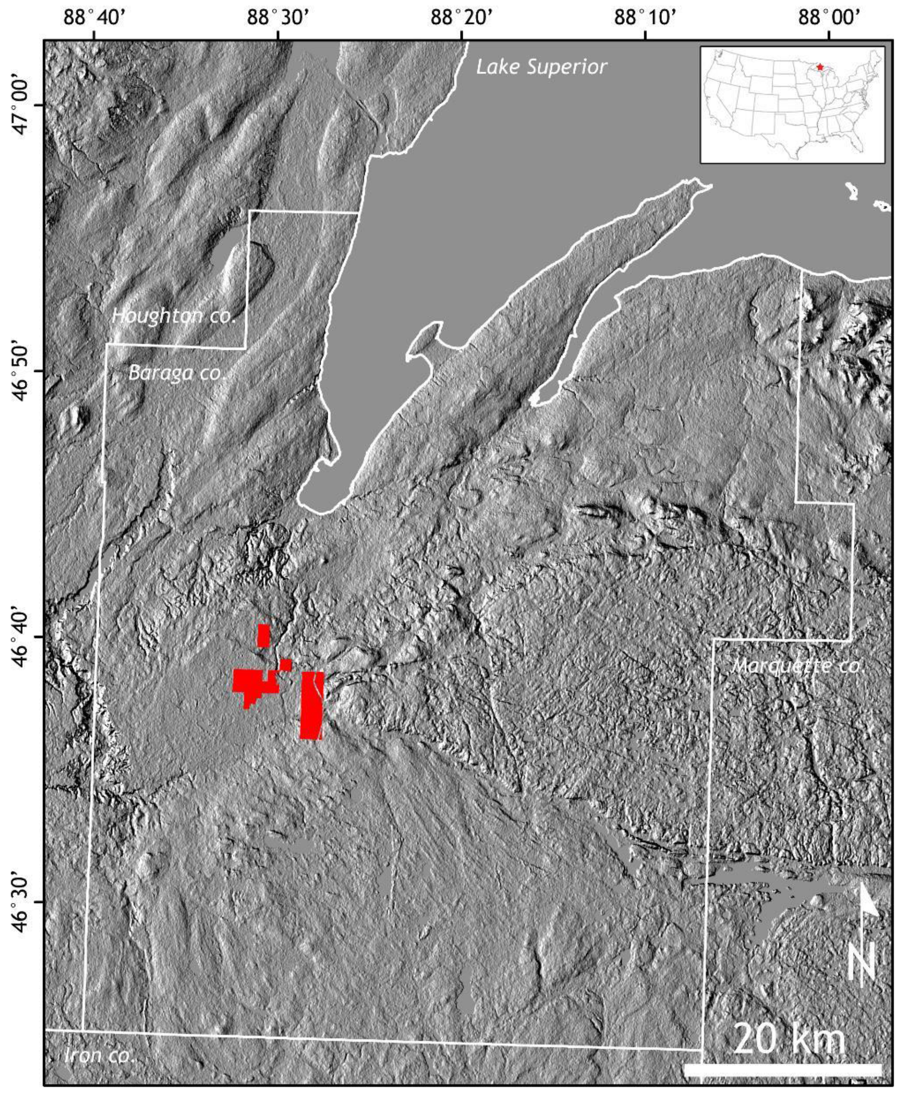
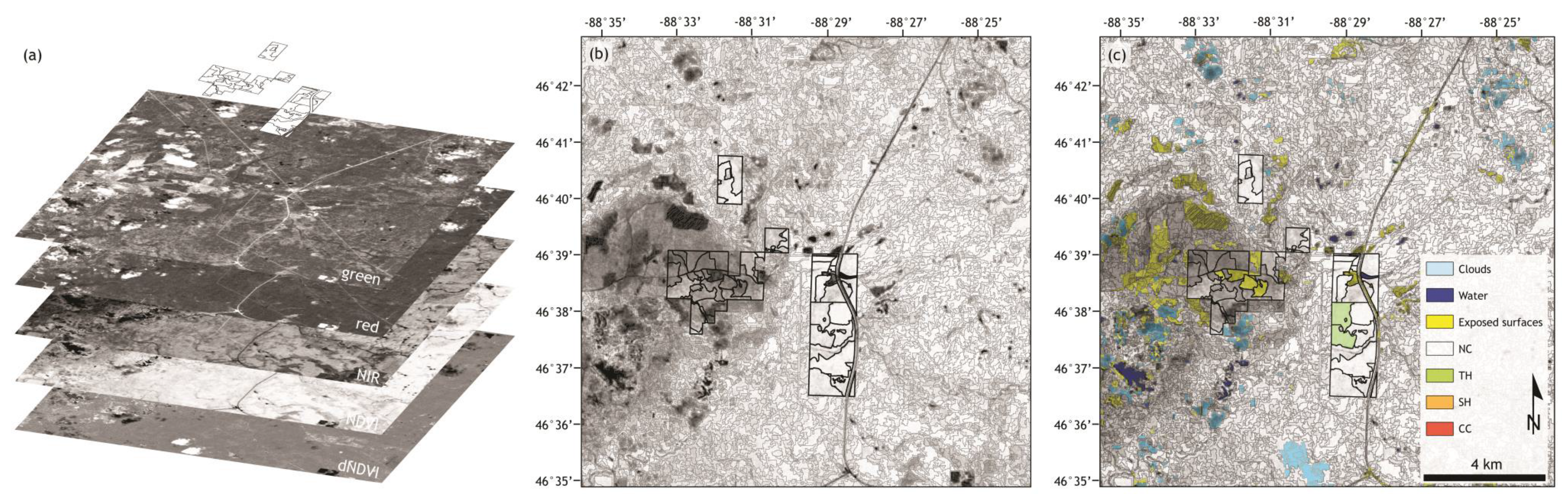
2. Study Area and Dataset

The FFC (Figure 1) consists of a research forest, the historic village of Alberta, a conference center and a sawmill museum, covering 5500 acres (~2225 ha) of extensive hardwood and jack pine plain forests in the Western Upper Peninsula of Michigan (USA). The forest has been divided into 33 management units, which support several forest types (primarily stands of jack pine (Pinus banksiana) or mixed northern hardwoods of sugar maple (Acer saccharum)/yellow birch (Betula alleghaniensis)/American beech (Fagus grandifolia)/white ash (Fraxinus americana), along with some stands of red pine (Pinus resinosa) and other less common associations) of different age classes and management histories.
We selected one TM scene of the FCC (WRS coordinates 024–028) per year based on two criteria: minimal or no cloud contamination and acquisition during the peak growing season. However, given Landsat temporal resolution and the constant presence of atmospheric clouds aggravated by the proximity of our sites to Lake Superior [35], the timespan of the TM scenes selected in this work ranges from June to August. The TM sensor on the Landsat-4 and Landsat-5 satellites covers a 185 km wide swath with a 16-day revisit, providing six 30 m resolution spectral channels plus one 90 m thermal band. The TM scenes were downloaded from the USGS EarthExplorer online catalogue as L1T product, consisting of at-sensor radiance single spectral channels orthorectified using a DEM and co-registered. Dense time series, or “stacks”, of Landsat scenes have recently been used in temperate environments for detecting both long-term vegetation trends [36] and land cover transitions [37,38]. The main advantage of this approach is that the larger number of observations can allow long-term changes to be detected with greater sensitivity and reliability by comparison to conventional two-date change detection.
Given the design and the scale of the problem, an atmospheric compensation of each scene was performed using the ATCOR-2/3 model (Geosystems GmbH, Germering, Germany) in order to obtain surface reflectance values, and the Normalized Difference Vegetation Index (NDVI) and difference of NDVI (dNDVI) was calculated for each year [39]. In order to maintain a high compatibility with other satellite sensors (e.g., Terra ASTER, UK-DMC, SPOT), these two layers were stacked with green, red, and near-infrared (NIR) surface reflectance bands, without taking into account the information contained in the blue (i.e., TM band 1). This temporal sequence of yearly multilayer images (i.e., green, red, NIR, NDVI and dNDVI for each year of the study) allowed the detection of harvest location and intensity at the FCC from 2005 to 2011, the last year with TM scenes available for the target area.

3. OBCD Classification
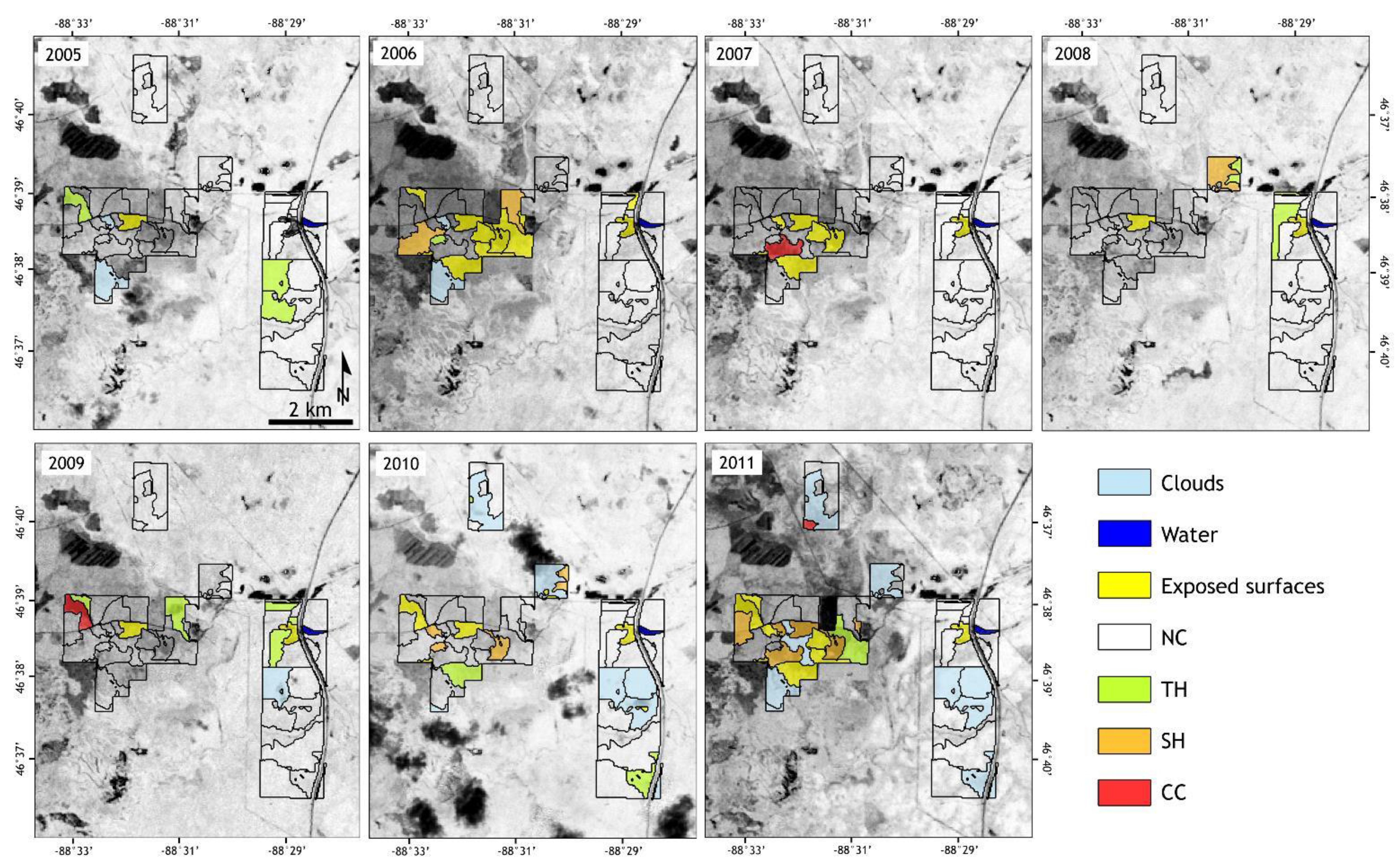
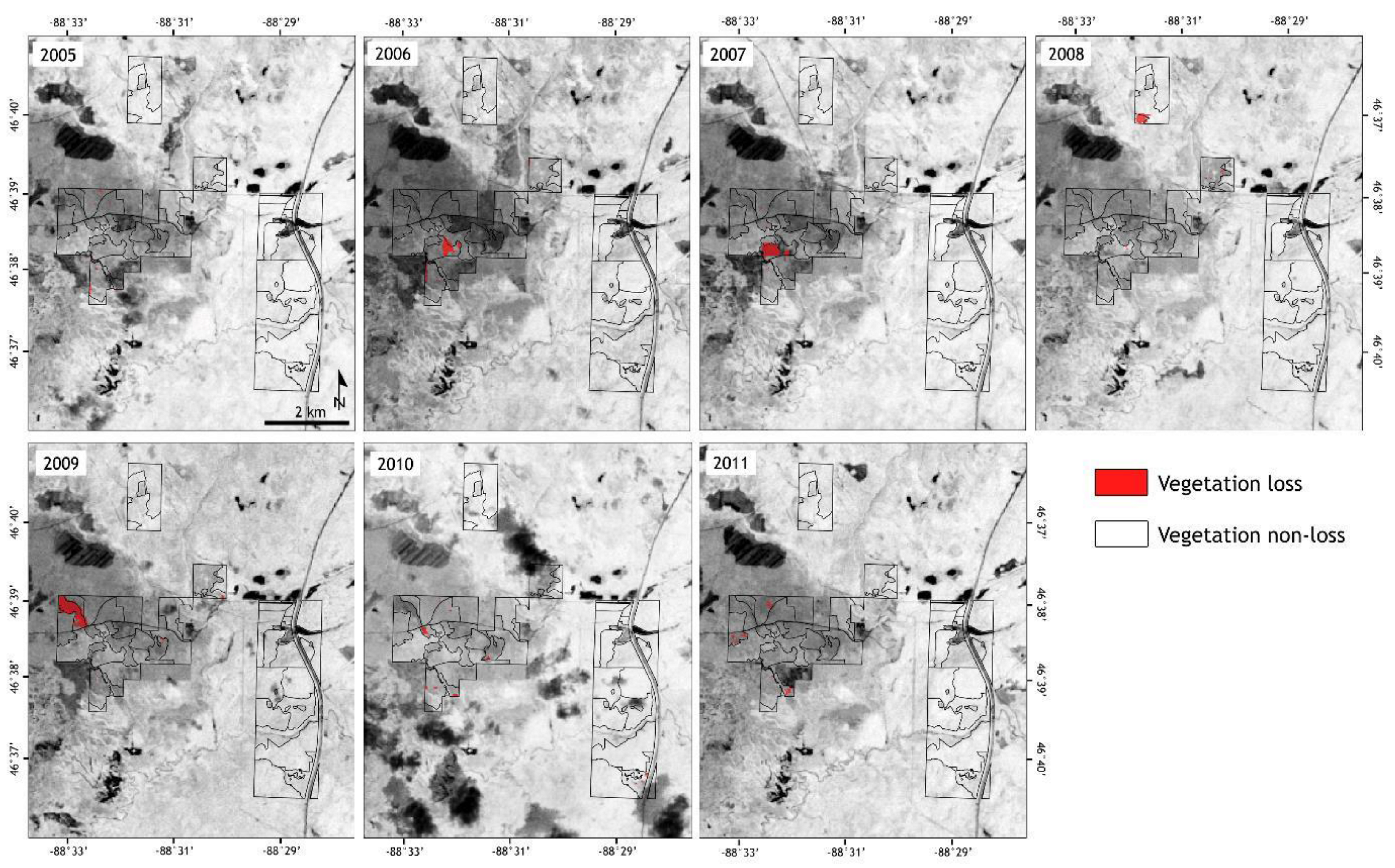
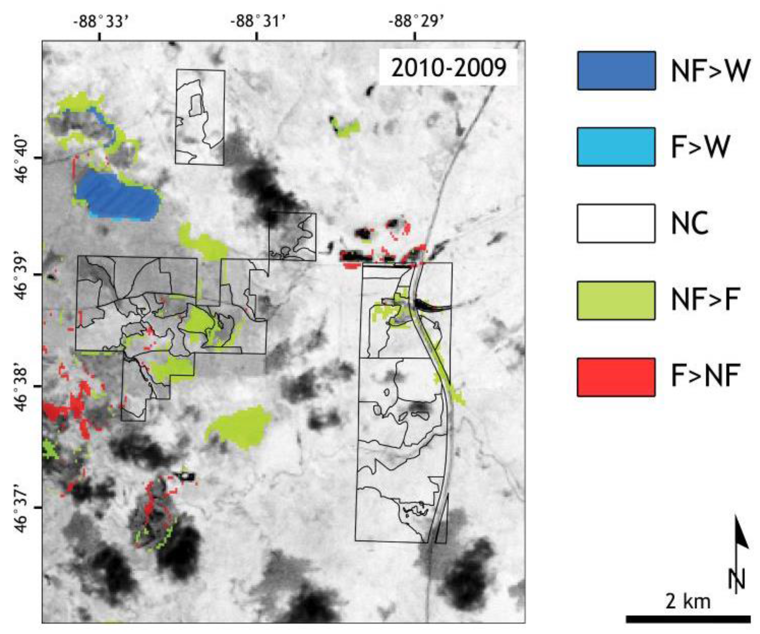
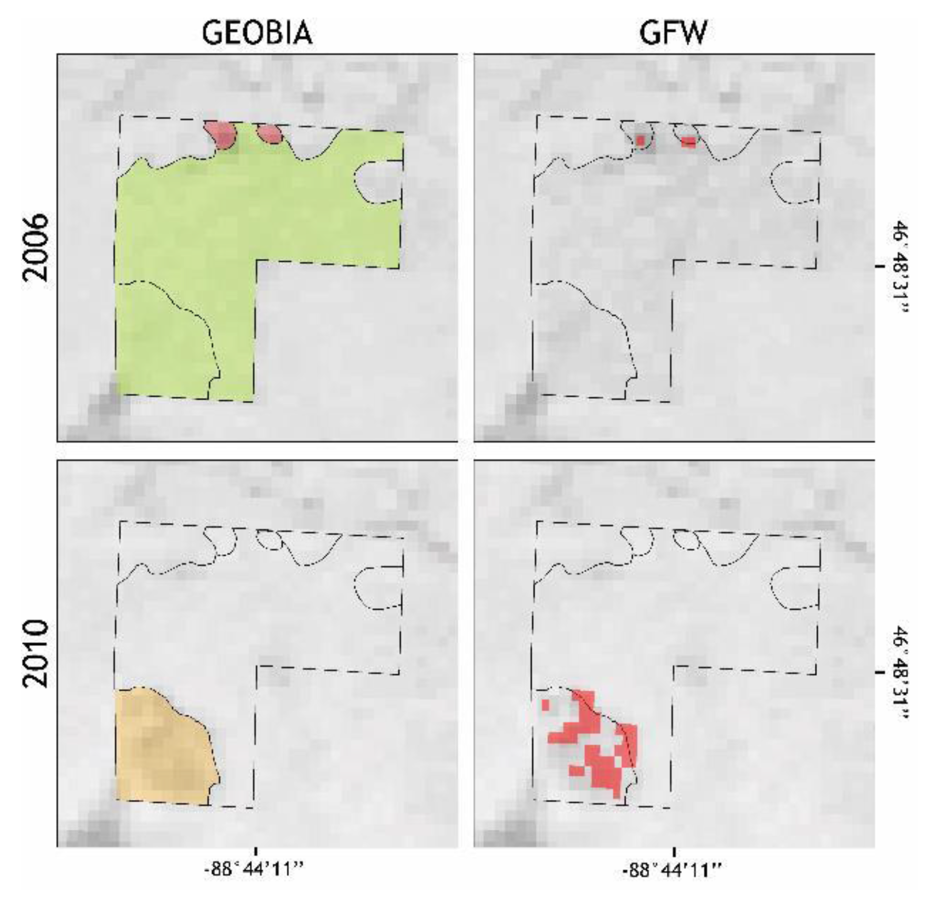
We utilize a class-object change detection algorithm [21] to identify and characterize harvests at the FFC. Although the NDVI has demonstrated to be sufficiently stable to permit meaningful comparisons of seasonal and inter-annual changes in vegetation growth and activity between years [40], the main disadvantage of the NDVI is the inherent nonlinearity of ratio-based indices and the influence of additive noise effects, such as atmospheric path radiances. Furthermore, the NDVI can also show scaling problems, asymptotic (saturated) signals over high biomass conditions, and is sensitive to canopy background variations [41]. Since we expected differences in the NDVI based on how much biomass had been removed in a harvest, for each possible harvest event we also registered year of occurrence and disturbance magnitude as difference with the previous year. On the other hand, an NDVI ratioing and/or differencing approach would reduce many forms of multiplicative noise (e.g., illumination differences, cloud shadows, atmospheric attenuation, certain topographic variations) that may have been present in multiple spectral bands [42]. For these reasons, we computed the year-by-year difference of the NDVI (i.e., dNDVI) as a preliminary step, to be included in the OBCD classification algorithm along with the green, red, NIR spectral bands, and NDVI (Figure 2a). In particular, on a year-by-year basis, the classes clouds, water and bare soil were defined in the first step of segmentation and classification of the images (Figure 2b), to produce a mask of “blank” objects for each image of the dataset.
Figure 2. Example of OBCD analysis of the 33 management units at the FFC and the surrounding area on the 2005 scene: (a) Input layers; (b) segments (gray) and unit boundaries (black); and (c) classification with legend.
Remotesensing 07 07809 g002
Although the atmospheric cloud coverage was minimal, the scenes used were not cloud-free. Therefore, yearly cloud masks had to be produced as a first step of the OBCD classification. Three parameters ruled the segmentation of each image. The scale parameter was representative of the maximum heterogeneity allowed in the segments and, therefore, controlled the size of the objects. The shape and compactness parameters controlled the outline and the dependency of objects to spectral and geometrical features [43]. In the first step, fixed parameters (i.e., scale: 15; shape: 0.1; compactness: 0.5) performed well in detecting atmospheric clouds in our dataset, these values are highly region-specific and may not work in other areas. The FFC units, outlined in a shapefile only containing the correct boundaries of the units within the FFC, were classified as clouds whenever intersected by a cloud segment, and these clouded areas were eliminated from further analyses.
Within the FFC boundary shapefile, a further class called vegetation was detected in the first step and in a second step subdivided into two sub-classes: change (C) and no change (NC), reflecting the expectation of a harvest or no harvest. The final step subdivided the class C into thinning (TH), selective harvest (SH), and clear cut (CC) (Figure 2c). These classes were established based on the percent of basal area (BA) harvested, derived from stand-level harvest data. In particular, BA removal percent for each class is defined as follows: 20 ≤ TH < 50, 50 ≤ SH < 80, 80 ≤ CC < 100. Figure 2 illustrates the entire classification process for the 2005 scene, and the OBCD classification thresholds are provided in the supplementary material. As our aim was to maximize the accuracy of the harvest intensity detection, the OBCD rulesets were optimized following this rationale.
Overall accuracy, user’s and producer’s accuracy, F1 score, and G-measure [44] were calculated to assess the accuracy of the OBCD classification. The overall accuracy measures the agreement between the events predicted to belong to a specific class (i.e., classification) and reference data (i.e., stand level observations). The user’s accuracy measures the proportion of objects classified as belonging to a class that are also labeled with that class in the reference data, while the producer’s accuracy measures the proportion of objects truly belonging to a class that are also classified as belonging to that class [45,46]. User’s and producer’s accuracies are related to commission (or false alarm) and omission errors as described in [47]. The F1 score and the G-measure are the harmonic and geometric mean of precision (i.e., producer’s accuracy) and recall (i.e., user’s accuracy) respectively, and represent a further assessment of the classification’s accuracy.
The OBCD algorithm utilized in this study was validated using external NIPF parcels within the same Landsat frame and harvested by Green Timber Consulting Foresters (Justin Miller, pers. comm.). The results of the OBCD classification at the FFC were compared to other pixel based classification products, such as the Landsat-based Global Forest Watch and ALOS PALSAR Forest/Non-Forest.

4. Results

The results of the OBCD classification are summarized in the supplementary material and shown in Figure 3. For accuracy assessment, the results of the classification were compared with the stand level classes of BA removal, including an error matrix of step 2 (i.e., C and NC detection, Table 1) and an overall accuracy assessment (Table 2).
Figure 3. Results of the OBCD classification overlaid onto the 2005–2011 NDVI dataset.
Remotesensing 07 07809 g003
Table 1. Error matrix of the C and NC detection.
Stand-Level
NCCtotal
PredictedNC2034207
C141024
Total21714231
Table 2. Accuracy assessment of the C and NC detection.
Producer’s AccuracyUser’s AccuracyCommission ErrorOmission ErrorF1 ScoreG-measure
NC0.980.950.050.020.960.96
C0.500.670.330.500.530.55
Other Landsat-based approaches, such as the Global Forest Watch vegetation loss data available from 2000 to 2012 [30], were found to be less accurate at predicting small harvesting events. The Global Forest Watch only detected three disturbance events at the FFC (Figure 4). In particular, the approach only detected two harvests (i.e., unit 15 in 2007; unit 17 in 2009), both clear cuts. Unit 33 in 2008 was misclassified as having vegetation loss, but stand-level BA% removal was 0. These results suggest that the Global Forest Watch can detect CC disturbances, but is less effective for less intense events (i.e., SH and TH) that still may represent a substantial loss (or gain) of forest biomass, particularly in the understory.
We validated our method using NIPF data within the same Landsat frame and harvested by Green Timber Consulting Foresters during our study period. The Validation Unit (VU) included five stands for a total extent of ~131 acres (~53 ha) and was representative of the three types of harvest detected with our method (Table 3; Figure 5). As with the FFC data, the Global Forest Watch detected only the CC harvest that occurred in the VU in 2006, and partially detected the SH that occurred in 2010. However, as for the FFC, TH harvests were not detected by the Global Forest Watch on these NIPF sites (Figure 5).
Other multi-temporal products, such as the ALOS PALSAR Forest/Non-Forest data available from 2007 to 2010 [34], were also found to be less effective for detecting small harvests. As an example, we show a map of the Forest/Non-Forest data for the years 2009 and 2010 (Figure 6). In general, only sparse and unclustered pixels show a change from 2009 to 2010, and most of them are edge pixels (i.e., there was a mismatch of the shape of the classification in the two contiguous years considered). However, both unit 12 and 26 are classified as Non-Forest in 2009 and Forest in 2010 (Figure 6). Although no change was recorded in our reference data in these units for those years, this is in accordance with the results obtained with our method (cf. Figure 3). Furthermore, a misclassification of a linear feature (i.e., U.S. Highway 41) crossing the easternmost units of the FFC is noticeable in Figure 6, and a pond was misclassified in 2009 as Non-Forest instead of Water. The large bean-shaped area in the northeastern section that was classified as either Non-Forest or Water (with noticeable striping in the 2010 image) was a large field that had been planted with annual rice to attract geese, suggesting that the PALSAR Forest/Non-Forest database may have some relevance to agricultural land uses.
Figure 4. Global Forest Watch classification overlaid onto the 2005–2011 NDVI dataset.
Remotesensing 07 07809 g004
Table 3. Description of the harvest events occurring in the VU.
YearForest TypeBA% Removal (class)Area (Acres)
2006Northern Hardwood20 (TH)102
2006Aspen100 (CC)2
2010Oak seed tree70 (SH)19
Figure 5. Comparison of OBCD and Global Forest Watch vegetation loss detection in the VU in 2006 and 2010, overlaid onto the corresponding NDVI image. Legend in accordance with Figure 3 and Figure 4, respectively.
Remotesensing 07 07809 g005
Figure 6. Difference of FNF classification in 2009 and 2010 at the FFC overlaid onto the 2010 NDVI image. Classes: non-forest to water (NF > W), forest > water (F > W), no change (NC), non-forest to forest (NF > F), forest to non-forest (F > NF).
Remotesensing 07 07809 g006

5. Discussion

The combination of an OBCD approach with remote sensing and ground-truthing data was able to identify not only where harvests have occurred in all forest types (i.e., northern hardwoods, mixed deciduous/coniferous, coniferous), but also the amount of woody biomass that was removed, down to ~20% BA for harvests as small as ~10 acres (approximately four Landsat pixels) with overall accuracy of 92%. The detection of C and NC events showed very high accuracies for the NC class (Table 2). However, in order to detect the largest number of disturbance events possible, our method tended to overestimate the number of harvests that occurred (i.e., commission error). This, combined with the different order of magnitude of the number of C and NC occurrences (i.e., 10 and >200, respectively), reflected a low producer’s accuracy of the class C (i.e., 50%; Table 1 and Table 2). The NDVI and dNDVI values may have also reflected some seasonal variability, translating to a less accurate classification in certain years. This may explain the SH class in 2011 (Figure 3), in which two SH events were not detected and four NC events are classified as SH (and one TH). This poor performance mostly depends on the different radiometry of each scene, but can also be related to a degradation of the quality of the data recorded by the TM sensor [48], in accordance with the lower accuracy obtained also in 2009 and 2010. In addition, potential incomplete harvesting (e.g., single harvest jobs spread over two or more years) could have also affected the accuracy of the classification.
By design, once a harvest is correctly detected (i.e., C is correctly classified), our method proved to be very accurate. Indeed, all the disturbance events (i.e., C events) that occurred between 2005 and 2010 were detected and classified with an overall accuracy of 100% (i.e., all the THs, SHs, and CCs were detected and classified correctly). Furthermore, our method performed very well in detecting NH disturbances, but was less for JP and mixed forest (cf. Supplementary Materials), possibly due to the naturally more open canopy of these forest communities.
Multi-date segmentation has recently received increasing attention for monitoring forest change [49], with studies using a variety of remote optical sensors at various spatial scales to detect and characterize disturbance and post-disturbance recovery of boreal, temperate and tropical forests (e.g., 25,50–53). Some of these studies demonstrated the effectiveness of the object-based approach for monitoring forest change using Landsat data, even detecting partial harvests. However, since our method only requires the green, red, and NIR spectral bands to identify and classify small harvests, the entire Landsat catalogue from 1972 (MSS) through the 1980s and 1990s (TM), along with other datasets with similar spatial resolutions and spectral band passes, can be utilized to measure trends in NIPF harvests over many decades, assuming that historical property boundary shapefiles are also available. Moreover, the Landsat-8 Operational Land Imager (OLI) is available from 2013, and other sensors (e.g., ASTER, DMC, SPOT) can be used to fill the 2012 gap in the Landsat legacy.
When applied at the state or regional level in the long term, this method can be used to measure the accuracy (in the aggregate) of the future plans recorded in the NWOS by private forest owners. As the NWOS has developed, several questions have prompted forest owners to predict how likely they are to perform certain management activities, including harvesting (and harvest intensity), along with other values and motivations for forest ownership [54]. Using this methodology, the number of owners reporting the intent to harvest in the next 5–10 years could be checked against the number of harvests (and their intensity) that actually occurred during that time in that survey area, providing an estimate of how closely landowner intentions match reality. Understanding the accuracy of these intentions will allow for more confidence in modeling future harvest rates, particularly when combined with the vast literature on the economic and environmental motivations of these owners [55,56]. Previous efforts to cross-check NWOS results have also used additional data, such as Forest Inventory and Analysis data, to examine forest characteristics across owners who differed in reasons for owning forests [57], however our method can provide an independent verification with finer temporal resolution (i.e., annual). Additionally, landscape-scale harvesting patterns such as clustering (often due to loggers preference for working in one area at a time) can be identified and monitored, and along with their impacts on water quality, road traffic, and other concerns.

6. Conclusions

In this work, we use an annual series of Landsat-5 TM scenes and a GIS shapefile of property boundaries to identify NIPF units where harvests occurred from 2005 to 2011, using an OBCD approach. Percent of basal area harvested was verified using stand-level harvest data. Our method detected all harvests above 20% basal area removal with a resolution of about 10% basal area in all forest types (northern hardwoods, mixed deciduous/coniferous, coniferous) on properties as small as 10 acres (approximately four Landsat pixels). This method could be extended to regional scales to identify small-scale and low intensity forest harvesting, typical of NIPF owners.
Monitoring forest harvesting is important to many scientific areas of inquiry, including climate change modeling (especially carbon cycling), estimations of biodiversity decline (through loss of forest habitats), and economic impacts (from trade in timber and wood products). Satellite images are excellent sources of information for land cover change, but without additional information, these changes cannot be reliably attributed to harvesting activities. However, relying solely on ground-truth data to verify remote sensing classification would require a prohibitive amount of surveying at larger scales. The assistance of the OBCD reduces the ground-truth data requirements and allows for small-scale harvest classifications over large areas. In this work, we illustrated how the use of ancillary data (such as property boundaries) in combination with satellite images allows small harvests to be identified much more reliably.

Acknowledgments

The authors wish to thank Justin Miller (Green Timber Consulting Foresters), the Western Upper Peninsula Planning and Development Region office, James Rivard and James Schmierer for data and advice, and Dirk Pflugmacher and Freek van der Meer and three anonymous reviewers for thoughtful comments on an earlier version of the manuscript. We are also grateful to the U.S. Geological Survey for providing Landsat data free of charge. This research was partially funded by the McIntyre-Stennis program administered by the U.S. Department of Agriculture—Forest Service to ALM.

Author Contributions

Riccardo Tortini was responsible for the acquisition and analysis of the satellite data, interpretation and validation of the results, and drafting of the manuscript; Audrey L. Mayer for the design and the NIPF harvesting implications of our research, and main technical guidance; and Pieralberto Maianti for calibration and processing of the OBCD algorithm. All authors have revised and approve the final version of the manuscript to be published.

Conflicts of Interest

The authors declare no conflict of interest.

References

  1. Hurtt, G.C.; Chini, L.P.; Frolking, S.; Betts, R.A.; Feddema, J.; Fischer, G.; Fisk, J.P.; Hibbard, K.; Houghton, R.A.; Janetos, A.; et al. Harmonization of land-use scenarios for the period 1500–2100: 600 Years of global gridded annual land-use transitions, wood harvest, and resulting secondary lands. Clim. Chang. 2011, 109, 117–161. [Google Scholar] [CrossRef]
  2. Smith, S.J.; Rothwell, A. Carbon density and anthropogenic land-use influences on net land-use change emissions. Biogeosciences 2013, 10, 6323–6337. [Google Scholar] [CrossRef] [Green Version]
  3. Edwards, D.P.; Gilroy, J.J.; Woodcock, P.; Edwards, F.A.; Larsen, T.H.; Andrews, D.J.R.; Derhe, M.A.; Docherty, T.D.S.; Hsu, W.W.; Mitchell, S.L.; et al. Land-sharing versus land-sparing logging: Reconciling timber extraction with biodiversity conservation. Glob. Chang. Biol. 2014, 20, 183–191. [Google Scholar] [CrossRef]
  4. Fischer, A.P.; Bliss, J.; Ingemarson, F.; Lidestav, G.; Lönnstedt, L. From the small woodland problem to ecosocial systems: The evolution of social research on small-scale forestry in Sweden and the USA. Scand. J. For. Res. 2010, 25, 390–398. [Google Scholar] [CrossRef]
  5. Mayer, A.L.; Rouleau, M.D. ForestSim model of impacts of smallholder dynamics: Forested landscapes of the Upper Peninsula of Michigan. Int. J. For. Res. 2013, 2013, 520207. [Google Scholar] [CrossRef]
  6. Butler, B.J. Family Forest Owners of the United States, 2006; Gen. Tech. Rep. NRS-27; U.S. Department of Agriculture, Forest Service, Northern Research Station: Newton Square, PA, USA, 2008; p. 72. [Google Scholar]
  7. Gustafson, E.J.; Loehle, C. Effects of parcelization and land divestiture on forest sustainability in simulated forest landscapes. For. Ecol. Manag. 2006, 236, 305–314. [Google Scholar] [CrossRef]
  8. Haines, A.L.; Kennedy, T.T.; McFarlane, D.L. Parcelization: Forest change agent in northern Wisconsin. J. For. 2011, 109, 101–108. [Google Scholar]
  9. Seymour, R.S.; White, A.S.; deMaynadier, P.G. Natural disturbance regimes in northeastern North America—Evaluating silvicultural systems using natural scales and frequencies. For. Ecol. Manag. 2002, 155, 357–367. [Google Scholar] [CrossRef]
  10. Kittredge, D.B.; Finley, A.O.; Foster, D.R. Timber harvesting as ongoing disturbance in a landscape of diverse ownership. For. Ecol. Manag. 2003, 180, 425–442. [Google Scholar] [CrossRef]
  11. Odum, W.E. Environmental degradation and the tyranny of small decisions. BioScience 1982, 32, 728–729. [Google Scholar] [CrossRef]
  12. Petrzelka, P.; Ma, Z.; Malin, S. The elephant in the room: Absentee landowner issues in conservation and management. Land Use Policy 2013, 30, 157–166. [Google Scholar] [CrossRef]
  13. Stone, R.N. 1970 A Comparison of Woodland Owner Intent with Woodland Practice in Michigan’s Upper Peninsula. Ph.D. Thesis, University of Minnesota, St. Paul, MN, USA, 1970. [Google Scholar]
  14. Franklin, S.E.; Lavigne, M.B.; Wulder, M.A.; Stenhouse, G.B. Change detection and landscape structure mapping using remote sensing. For. Chron. 2002, 78, 618–625. [Google Scholar] [CrossRef]
  15. Pocock, M.J.O.; Evans, D.M.; Memmott, J. The impact of farm management on species-specific leaf area index (LAI): Farm-scale data and predictive models. Agric. Ecosyst. Environ. 2010, 135, 279–287. [Google Scholar] [CrossRef]
  16. Binford, M.W.; Gholz, H.L.; Starr, G.; Martin, T.A. Regional carbon dynamics in the southeastern U.S. coastal plain: Balancing land cover type, timber harvesting, fire, and environmental variation. J. Geophys. Res.: Atmos. 2006, 111, D24S92. [Google Scholar] [CrossRef]
  17. Baker, B.A.; Warner, T.A.; Conley, J.F.; McNeil, B.E. Does spatial resolution matter? A multi-scale comparison of object-based and pixel-based methods for detecting change associated with gas well drilling operations. Int. J. Remote Sens. 2013, 34, 1633–1651. [Google Scholar] [CrossRef]
  18. Schiewe, J. Segmentation of high-resolution remotely sensed data: Concepts, applications and problems. Int. Arch. Photogramm. Remote Sens. Spat. Sci. Inf. 2002, 34, 380–385. [Google Scholar]
  19. Blaschke, T.; Lang, S.; Lorup, E.; Strobl, J.; Zeil, P. Object-oriented image processing in an integrated GIS/remote sensing environment and perspectives for environmental applications. Environ. Inf. Plan. Polit. Public 2000, 2, 555–570. [Google Scholar]
  20. Blaschke, T. Object based image analysis for remote sensing. ISPRS J. Photogramm. Remote Sens. 2010, 65, 2–16. [Google Scholar] [CrossRef]
  21. Chen, G.; Hay, G.J.; Carvalho, L.M.T.; Wulder, M.A. Object-based change detection. Int. J. Remote Sens. 2012, 33, 37–41. [Google Scholar] [CrossRef]
  22. Chen, G.; Zhao, K.; Powers, R. Assessment of the image misregistration effects on object-based change detection. ISPRS J. Photogramm. Remote Sens. 2014, 87, 19–27. [Google Scholar] [CrossRef]
  23. Heumann, B.W. An object-based classification of mangroves using a hybrid decision tree—Support vector machine approach. Remote Sens. 2011, 3, 2440–2460. [Google Scholar] [CrossRef]
  24. Dao, P.D.; Liou, Y.-A. Object-based flood mapping and affected rice field estimation with Landsat 8 OLI and MODIS data. Remote Sens. 2015, 7, 5077–5097. [Google Scholar] [CrossRef]
  25. Hall, O.; Hay, G.J. A multiscale object-specific approach to digital change detection. Int. J. Appl. Earth Obs. Geoinf. 2003, 4, 311–327. [Google Scholar] [CrossRef]
  26. Blaschke, T. Towards a framework for change detection based on image objects. In Remote Sensing & GIS for Environmental Studies: Applications in Geography; Erasmi, S., Cyffka, B., Kappas, M., Eds.; Göttinger Geographische Abhandlungen: Göttingen, Germany, 2005; Volume 113, pp. 1–9. [Google Scholar]
  27. Hay, G.J.; Castilla, G. Geographic Object-Based Image Analysis (GEOBIA): A new name for a new discipline. In Object Based Image Analysis—Spatial Concepts for Knowledge-Driven Remote Sensing Applications; Blaschke, T., Lang, S., Hay, G.J., Eds.; Springer-Verlag: Heidelberg, Germany, 2008; pp. 75–85. [Google Scholar]
  28. Townshend, J.R.G.; Justice, C.O. The spatial variation of vegetation at very large scales. Int. J. Remote Sens. 1990, 11, 149–157. [Google Scholar] [CrossRef]
  29. Goward, S.N.; Williams, D.L. Landsat and Earth systems science: Development of terrestrial monitoring. Photogramm. Eng. Remote Sens. 1997, 63, 887–900. [Google Scholar]
  30. Hansen, M.C.; Potapov, P.V.; Moore, R.; Hancher, M.; Turubanova, S.A.; Tyukavina, A.; Thau, D.; Stehman, S.V.; Goetz, S.J.; Loveland, T.R.; et al. High-resolution global maps of 21st century forest cover change. Science 2013, 342, 850–853. [Google Scholar] [CrossRef]
  31. Singh, A. Digital change detection techniques using remotely-sensed data. Int. J. Remote Sens. 1989, 10, 989–1003. [Google Scholar] [CrossRef]
  32. Lu, D.; Mausel, P.; Brondizio, E.; Moran, E. Change detection techniques. Int. J. Remote Sens. 2004, 25, 2365–2407. [Google Scholar] [CrossRef]
  33. Zhou, W.; Troy, A. An object-oriented approach for analysing and characterizing urban landscape at the parcel level. Int. J. Remote Sens. 2008, 29, 3119–3135. [Google Scholar] [CrossRef]
  34. Shimada, M.; Itoh, T.; Motooka, T.; Watanabe, M.; Shiraishi, T.; Thapa, R.; Lucas, R. New global forest/non-forest maps from ALOS PALSAR data (2007–2010). Remote Sens. Environ. 2014, 155, 13–31. [Google Scholar] [CrossRef]
  35. Scott, R.W.; Huff, F.A. Impacts of the Great Lakes on regional climate conditions. J. Great Lakes Res. 1996, 22, 845–863. [Google Scholar] [CrossRef]
  36. Röder, A.; Udelhoven, T.; Hill, J.; del Barrio, G.; Tsiourlis, G. Trend analysis of Landsat-TM and-ETM+ imagery to monitor grazing impact in a rangeland ecosystem in Northern Greece. Remote Sens. Environ. 2008, 112, 2863–2875. [Google Scholar] [CrossRef]
  37. Huang, C.; Goward, S.N.; Masek, J.G.; Thomas, N.; Zhu, Z.; Vogelmann, J.E. An automated approach for reconstructing recent forest disturbance history using dense Landsat time series stacks. Remote Sens. Environ. 2010, 114, 183–198. [Google Scholar] [CrossRef]
  38. Kennedy, R.E.; Yang, Z.; Cohen, W.B. Detecting trends in forest disturbance and recovery using yearly Landsat time series: 1. LandTrendr—Temporal segmentation algorithms. Remote Sens. Environ. 2010, 114, 2897–2910. [Google Scholar] [CrossRef]
  39. Rouse, J.W., Jr.; Haas, R.H.; Schell, J.A.; Deering, D.W. Monitoring vegetation systems in the Great Plains with ERTS. In Proceedings of the 3rd Earth Resources Technology Satellite-1, Washington, DC, USA, 10–14 December 1973; pp. 309–313.
  40. Huete, A.R.; Didan, K.; Miura, T.; Rodriguez, E.P.; Gao, X.; Ferreira, L.G. Overview of the radiometric and biophysical performance of the MODIS vegetation indices. Remote Sens. Environ. 2002, 83, 195–213. [Google Scholar] [CrossRef]
  41. Huete, A.R. A Soil-Adjusted Vegetation Index (SAVI). Remote Sens. Environ. 1988, 25, 295–309. [Google Scholar] [CrossRef]
  42. Liu, H.Q.; Huete, A.R. A feedback based modification of the NDVI to minimize canopy background and atmospheric noise. IEEE Trans. Geosci. Remote Sens. 1995, 33, 457–465. [Google Scholar]
  43. Maianti, P.; Rusmini, M.; Tortini, R.; Dalla Via, G.; Frassy, F.; Marchesi, A.; Rota Nodari, F.; Gianinetto, M. Monitoring large oil slick dynamics with moderate resolution multispectral satellite data. Nat. Hazards 2014, 73, 473–492. [Google Scholar] [CrossRef]
  44. Powers, D.M.W. Evaluation: From precision, recall and F-measure to ROC, informedness, markedness & correlation. J. Mach. Learn. Technol. 2011, 2, 37–63. [Google Scholar]
  45. Stehman, S.V.; Czaplewski, R.L. Design and analysis for thematic map accuracy assessment: Fundamental principles. Remote Sens. Environ. 1998, 64, 331–344. [Google Scholar] [CrossRef]
  46. Congalton, R.G. A review of assessing the accuracy of classifications of remotely sensed data. Remote Sens. Environ. 1991, 37, 35–46. [Google Scholar] [CrossRef]
  47. Janssen, L.L.F.; Wel, F. Accuracy assessment of satellite derived land cover data: A review. IEEE Photogramm. Eng. Remote Sens. 1994, 60, 419–426. [Google Scholar]
  48. Markham, B.L.; Storey, J.C.; Williams, D.L.; Irons, J.R. Landsat sensor performance: History and current status. IEEE Trans. Geosci. Remote Sens. 2004, 42, 2691–2694. [Google Scholar] [CrossRef]
  49. GOFC-GOLD. A Sourcebook of Methods and Procedures for Monitoring and Reporting Anthropogenic Greenhouse Gas Emissions and Removals Associated with Deforestation, Gains and Losses of Carbon Stocks in Forests Remaining Forests, and Forestation, GOFC-GOLD Report version COP18–1; GOFC-GOLD Land Cover Project Office, Wageningen University: Wageningen, The Netherlands, 2012. [Google Scholar]
  50. Desclée, B.; Bogaert, P.; Defourny, P. Forest change detection by statistical object-based method. Remote Sens. Environ. 2006, 102, 1–11. [Google Scholar] [CrossRef]
  51. Linke, J.; McDermid, G.J.; Laskin, D.N.; McLane, A.J.; Pape, A.; Cranston, J.; Hallbeyer, M.; Franklin, S.E. A disturbance-inventory framework for flexible and reliable landscape monitoring. Photogramm. Eng. Remote Sens. 2009, 75, 981–995. [Google Scholar] [CrossRef]
  52. Dorren, L.K.; Maier, B.; Seijmonsbergen, A.C. Improved Landsat-based forest mapping in steep mountainous terrain using object-based classification. For. Ecol. Manag. 2003, 183, 31–46. [Google Scholar] [CrossRef]
  53. Bontemps, S.; Bogaert, P.; Titeux, N.; Defourny, P. An object-based change detection method accounting for temporal dependences in time series with medium to coarse spatial resolution. Remote Sens. Environ. 2008, 112, 3181–3191. [Google Scholar] [CrossRef]
  54. Bengston, D.N.; Asah, S.T.; Butler, B.J. The diverse values and motivations of family forest owners in the United States: An analysis of an open-ended question in the National Woodland Owner Survey. Small-Scale For. 2011, 10, 339–355. [Google Scholar] [CrossRef]
  55. Beach, R.H.; Pattanayak, S.K.; Yang, J-C.; Murray, B.C.; Abt, R.C. Econometric studies of non-industrial private forest management: A review and synthesis. For. Policy Econ. 2005, 7, 261–281. [Google Scholar] [CrossRef]
  56. Butler, B.J.; Ma, Z. Family forest owner trends in the northern United States. North. J. Appl. For. 2011, 28, 13–18. [Google Scholar]
  57. Moser, W.K.; Leatherberry, E.C.; Hansen, M.H.; Butler, B.J. Farmers’ objectives toward their woodlands in the upper Midwest of the United States: Implications for woodland volumes and diversity. Agrofor. Syst. 2009, 75, 49–60. [Google Scholar] [CrossRef]

