
Drought Variability and Land Degradation in Semiarid Regions: Assessment Using Remote Sensing Data and Drought Indices (1982–2011)


Abstract
:
1. Introduction
2. Data and Methods
2.1. Datasets
2.1.1. Global Normalized Difference Vegetation Index
2.1.2. Drought Data
2.1.3. Other Data
2.2. Analysis
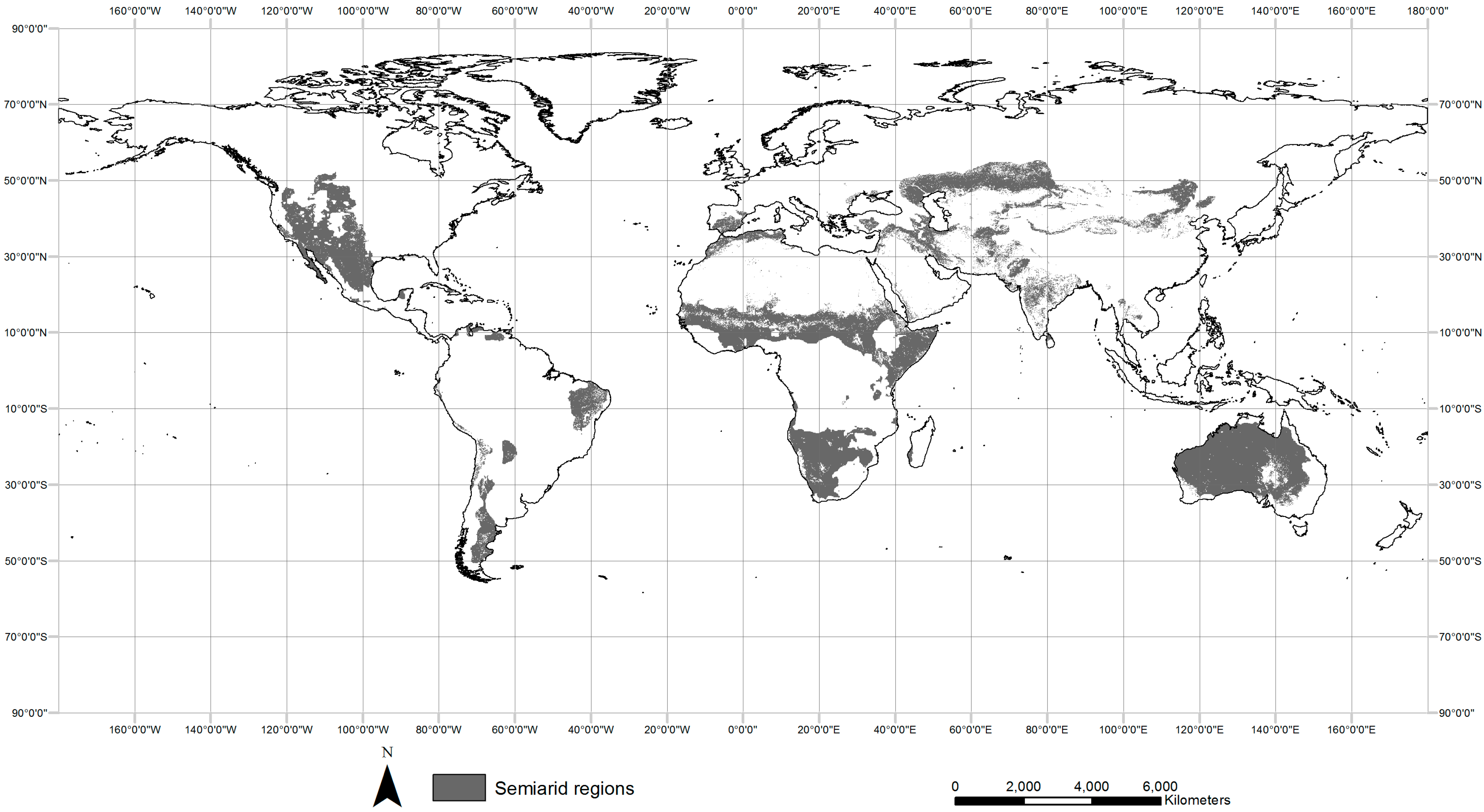
2.2.1. Identification of Semiarid Regions

2.2.2. Identification of the Month of Maximum Vegetation Activity (NDVImax)
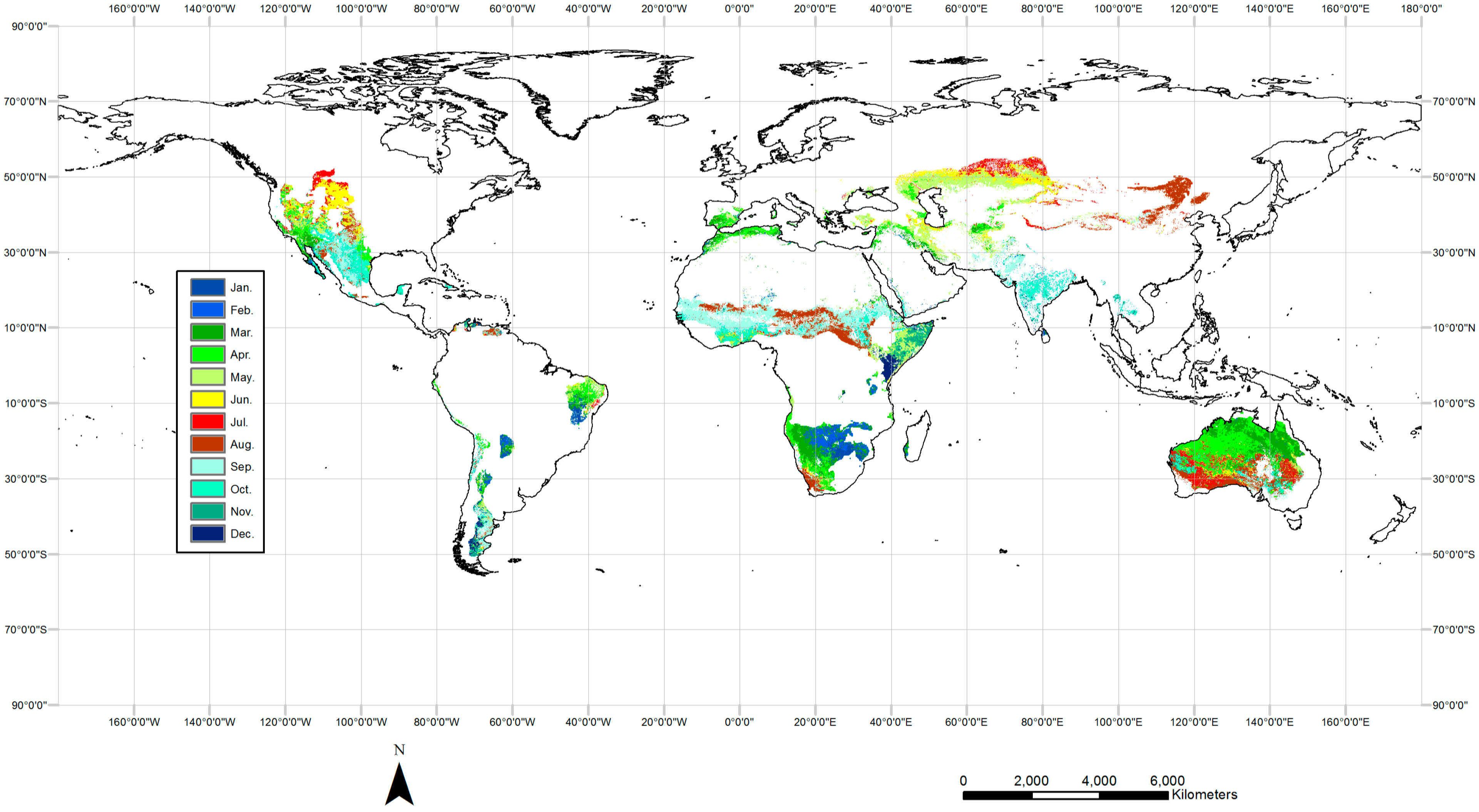
2.2.3. NDVImax Trends: Sign and Magnitude
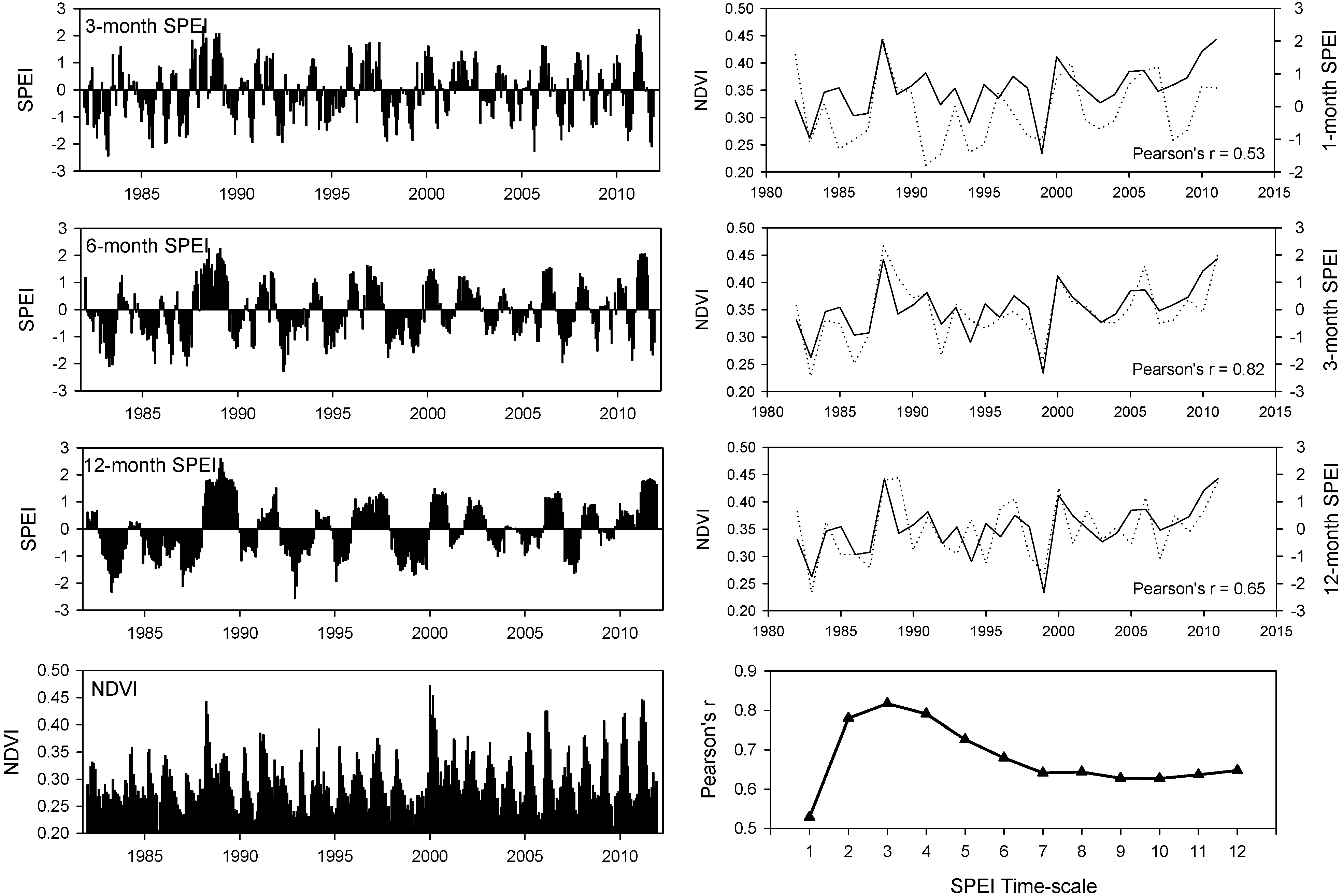
2.2.4. Time Scale of SPEI with Maximum Correlation between NDVImax and SPEI
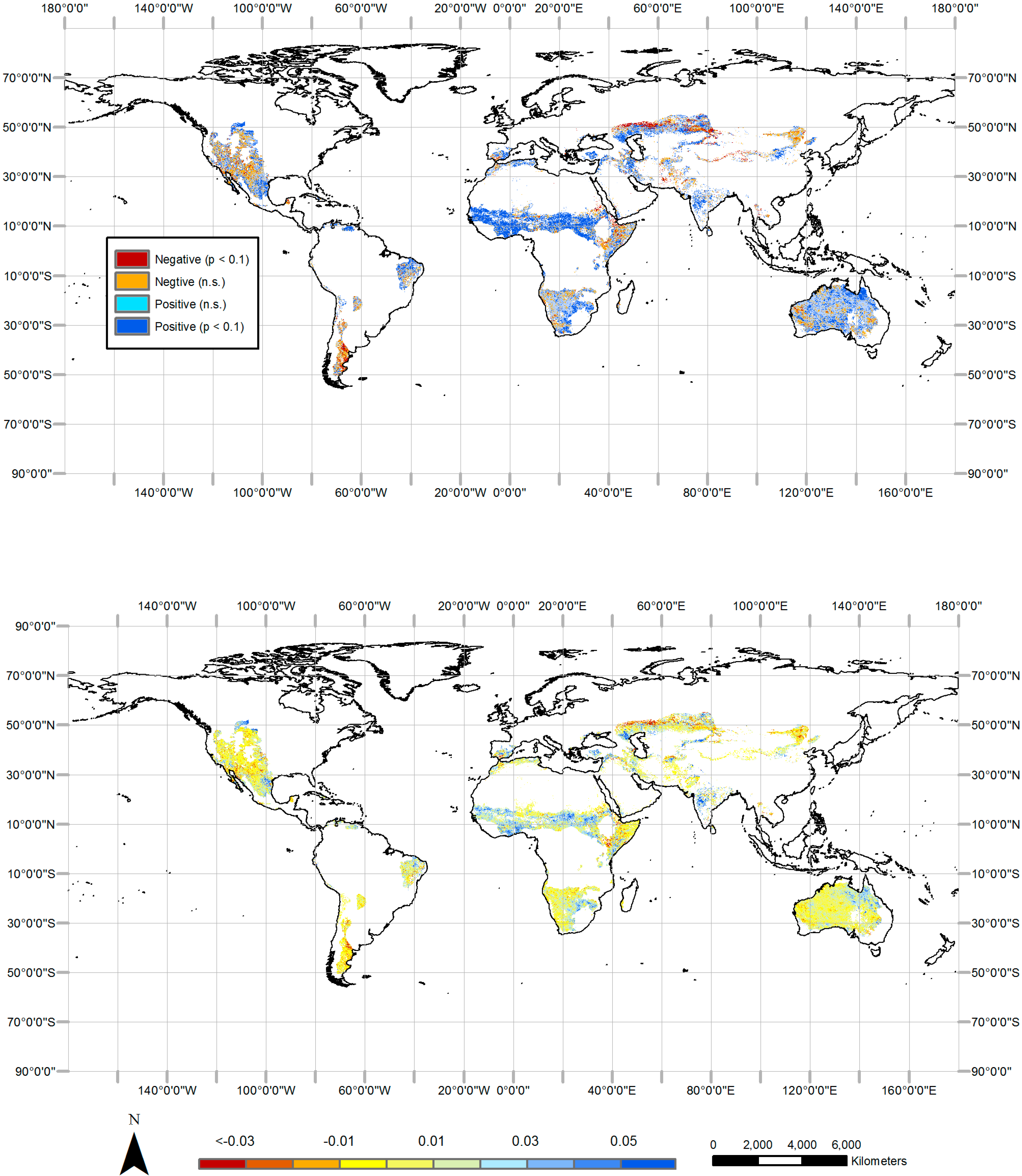
2.2.5. Relationship between NDVImax Trends and SPEI Trends
2.2.6. Regression Model NDVImax-SPEI
3. Results
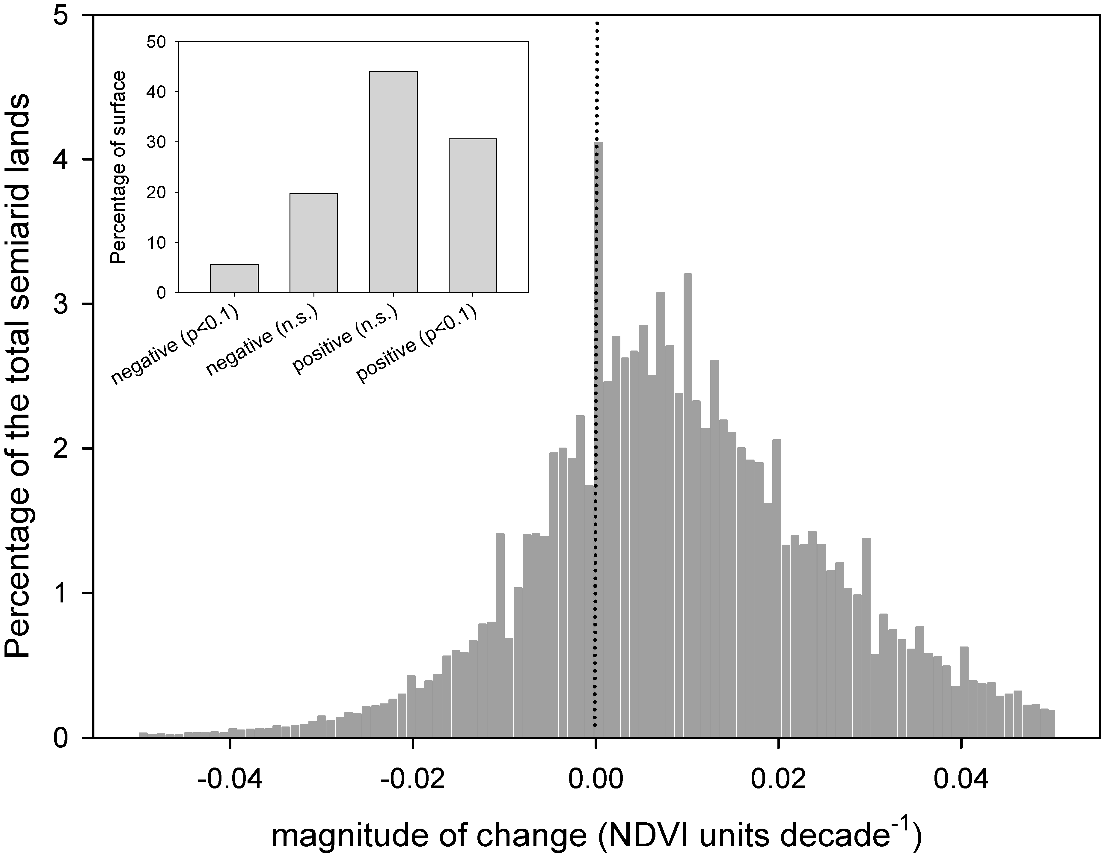
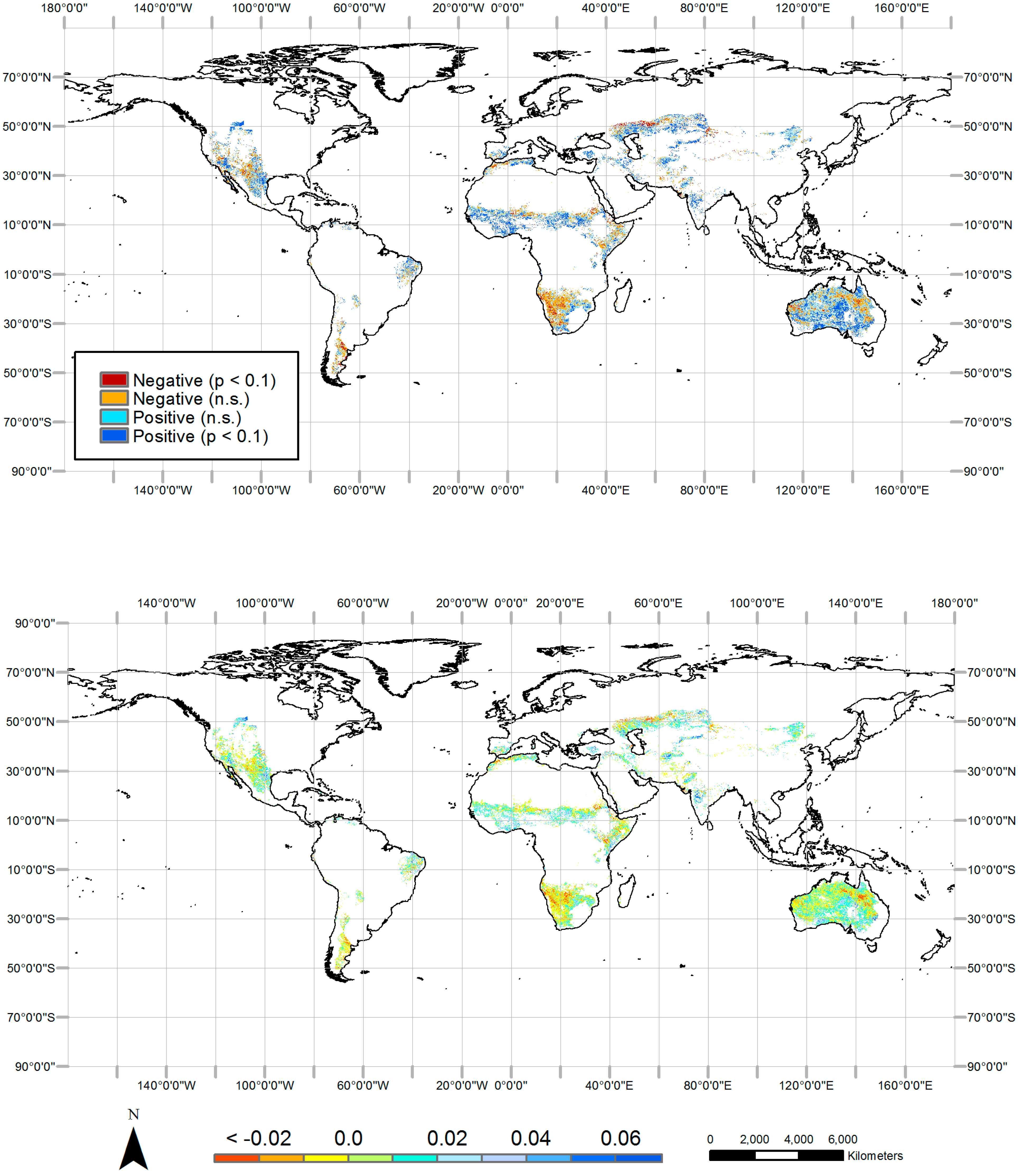
3.1. NDVImax Trends

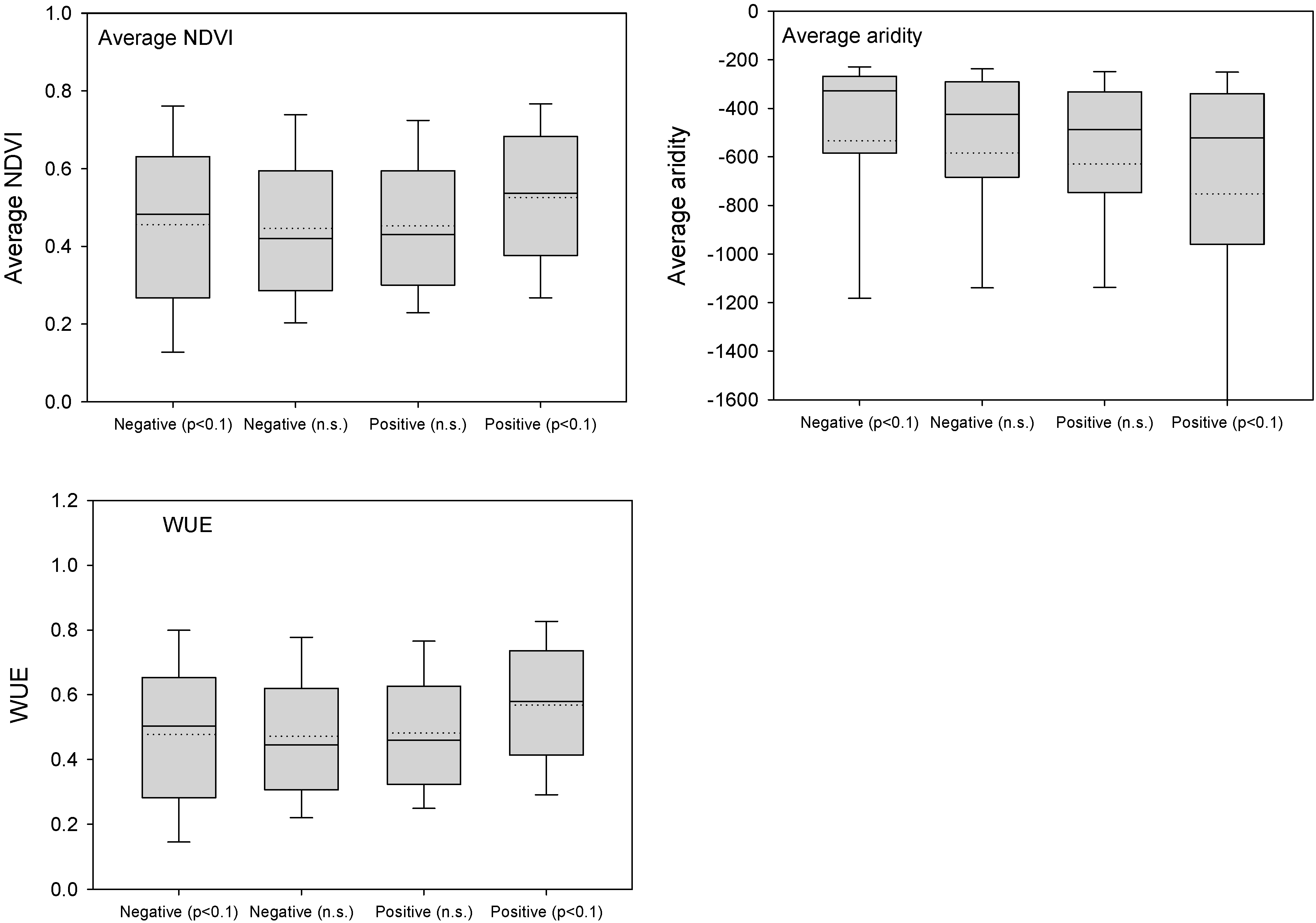
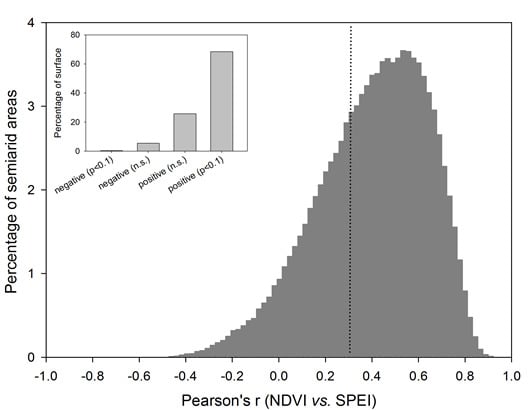
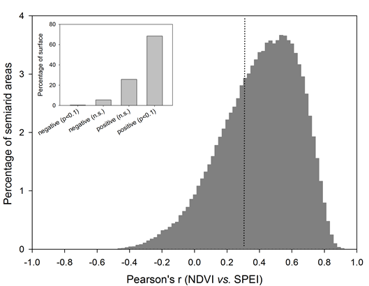
3.2. Drought Influence on NDVI Variability and Trends
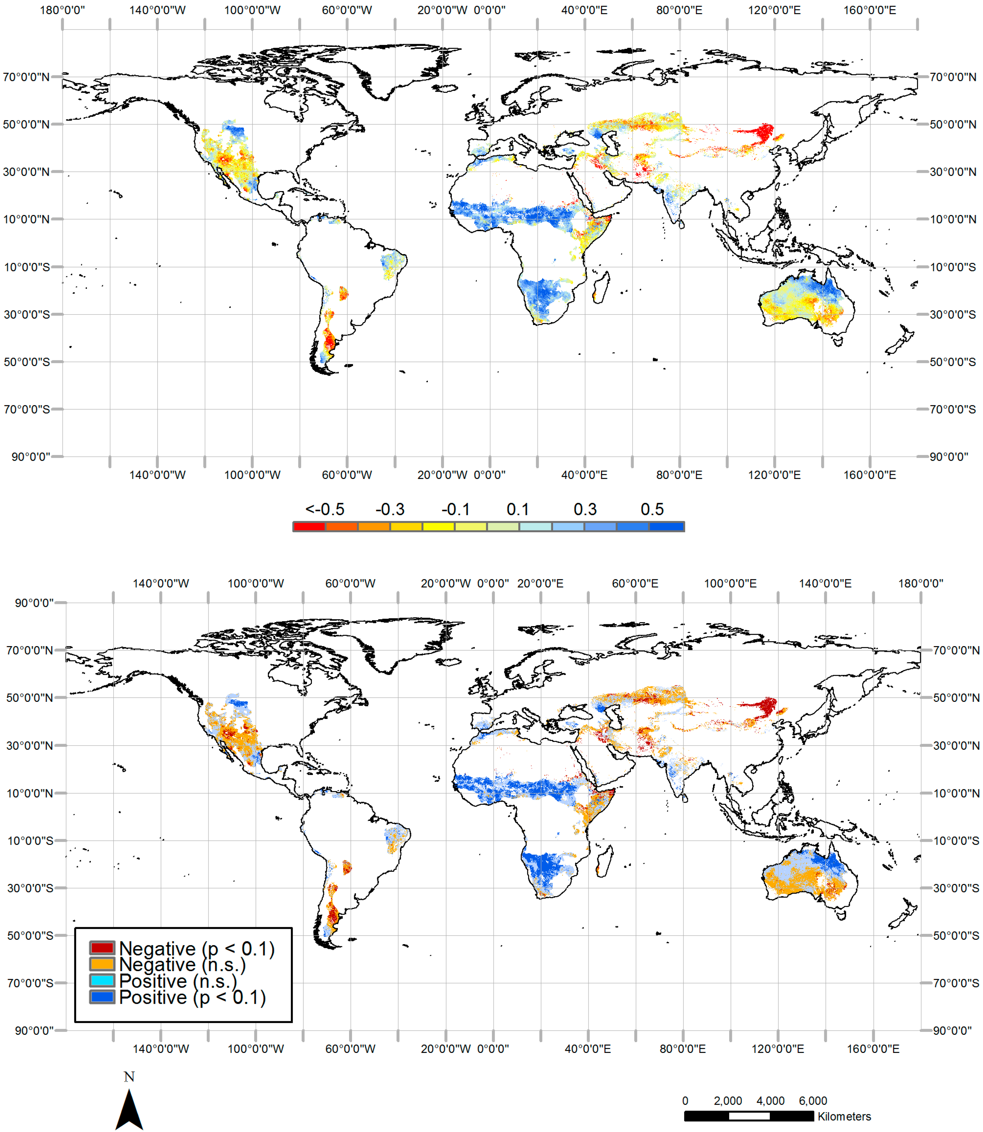
3.3. Trends in SPEI

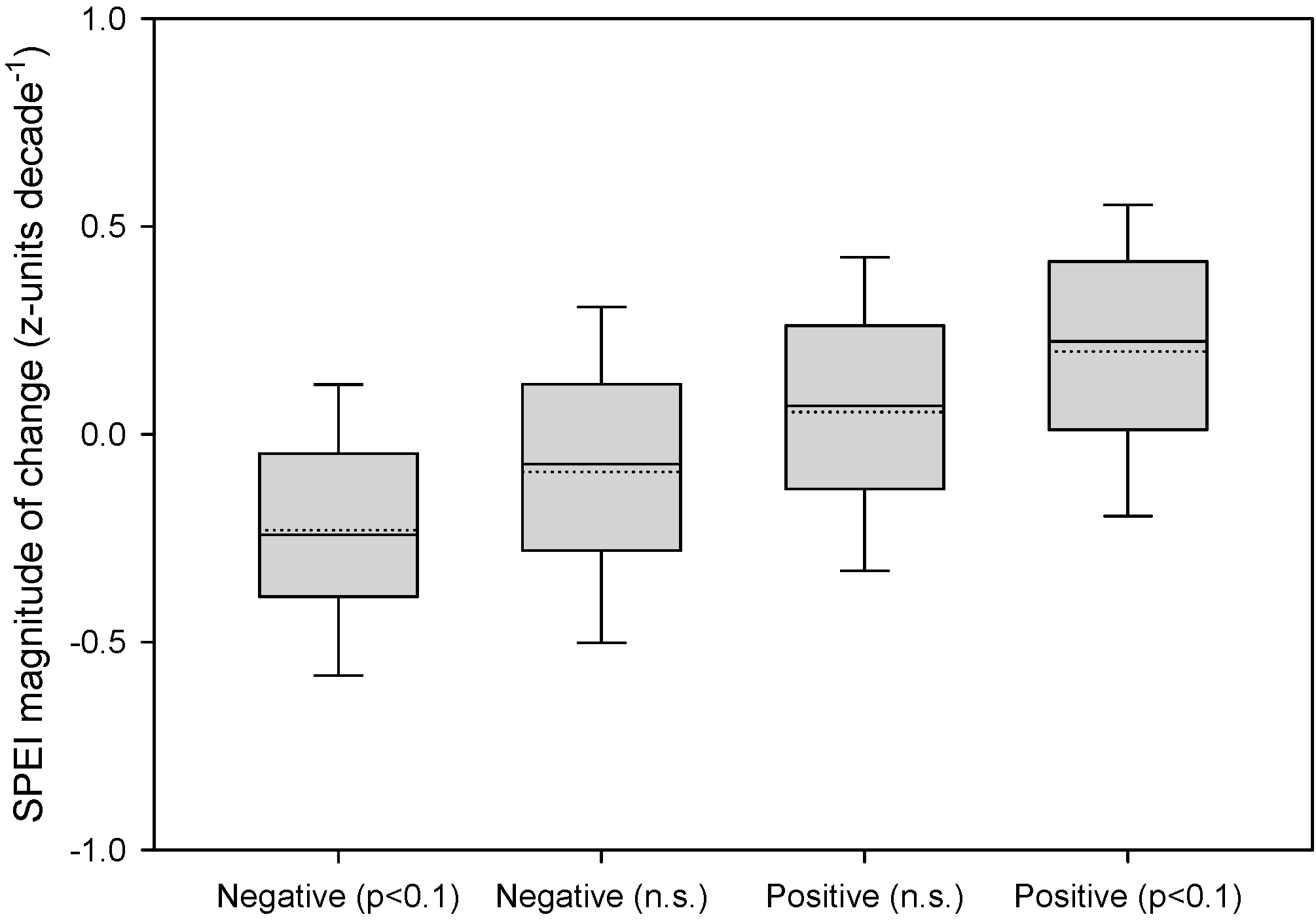
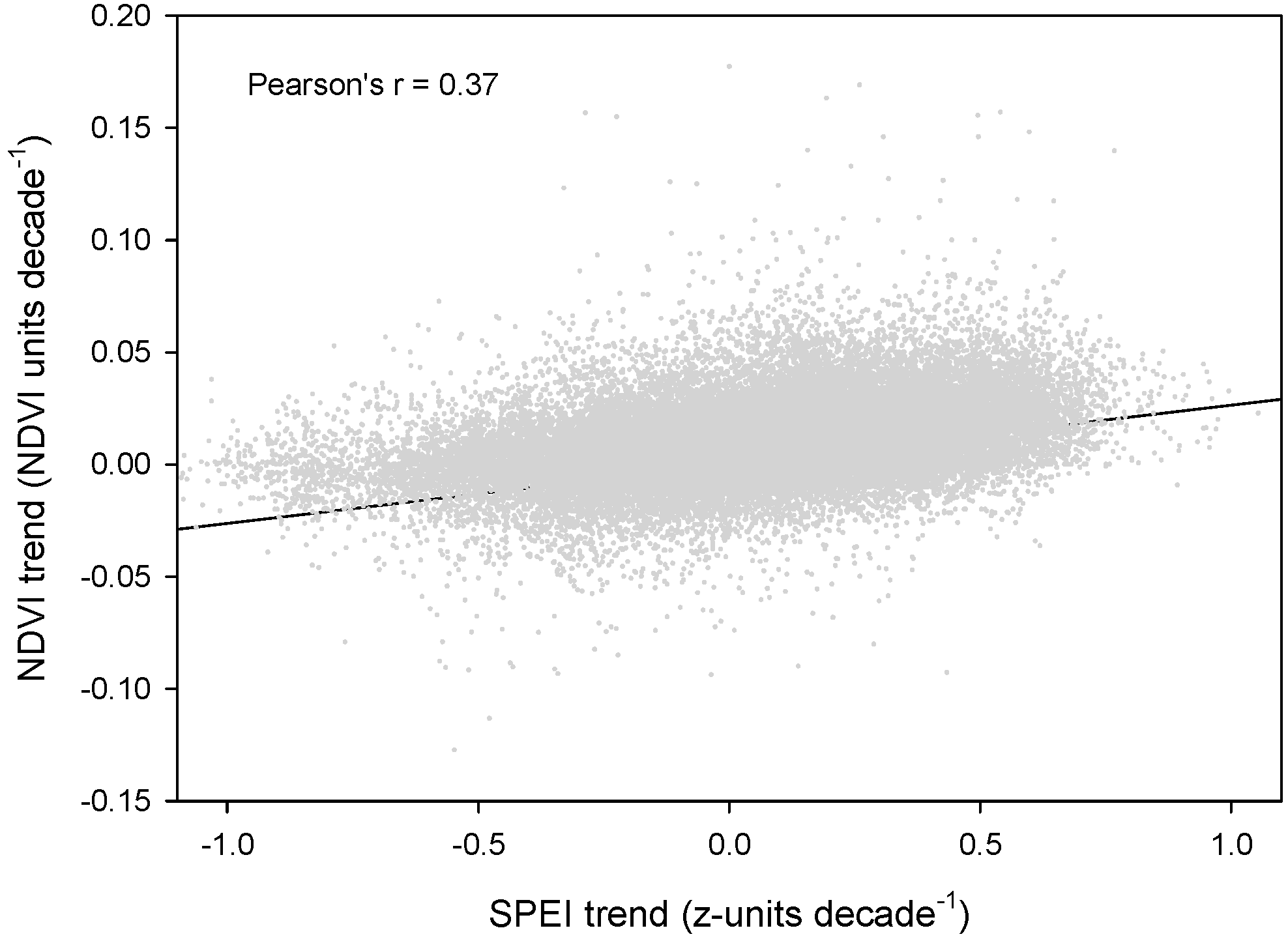
3.4. Relationship between SPEI Trends and NDVImax Trends


| Chi-Square | 5293,838 |
| sig | <0.000 |
| CC | 0.350 |
| sig | <0.000 |
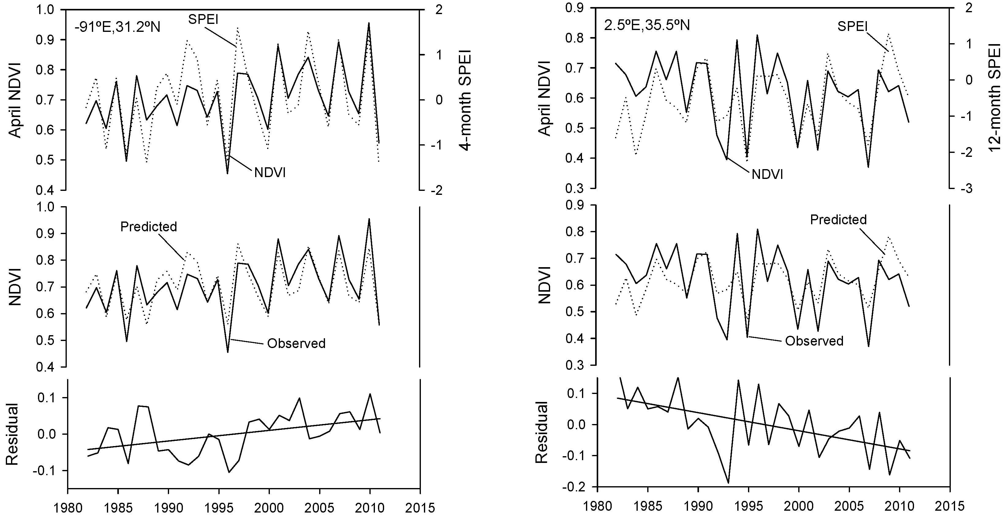
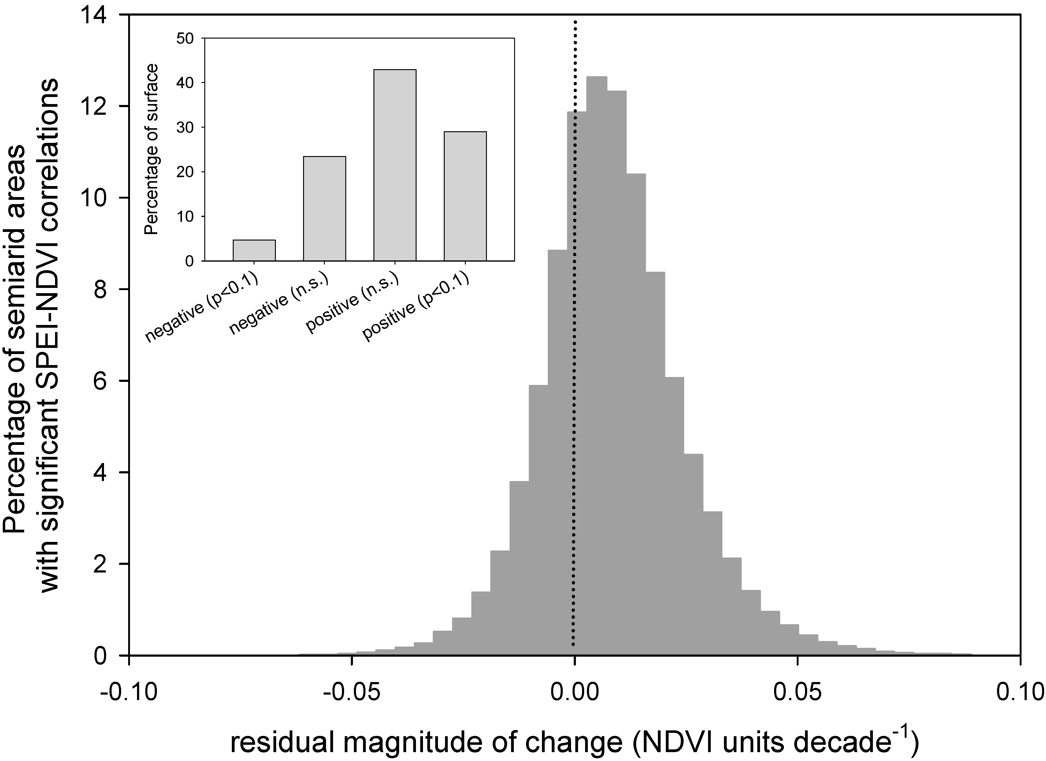
3.5. Evolution of Residual Series


4. Discussion
4.1. Vegetation Activity Trends
4.2. Influence of the Drought Variability on Vegetation Activity
4.3. Other Possible Explanatory Factors
5. Conclusions
- Positive trends in NDVImax clearly dominated across the world’s semiarid regions for the period 1982–2011.
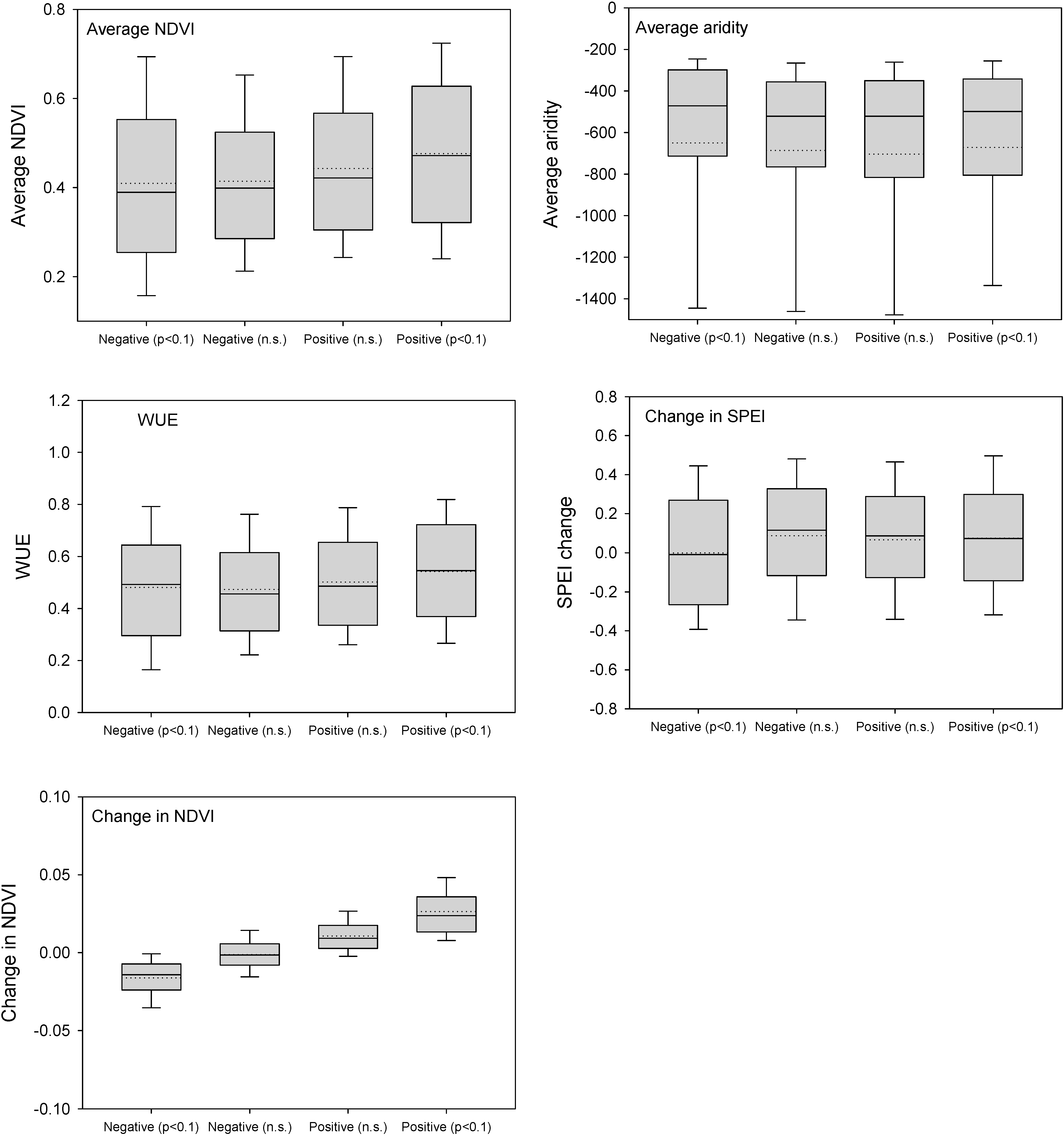
- Areas showing negative and significant trends in NDVImax mostly corresponded to areas associated with lower climate aridity, whereas the areas showing positive and significant NDVImax trends in general corresponded to the most arid regions.
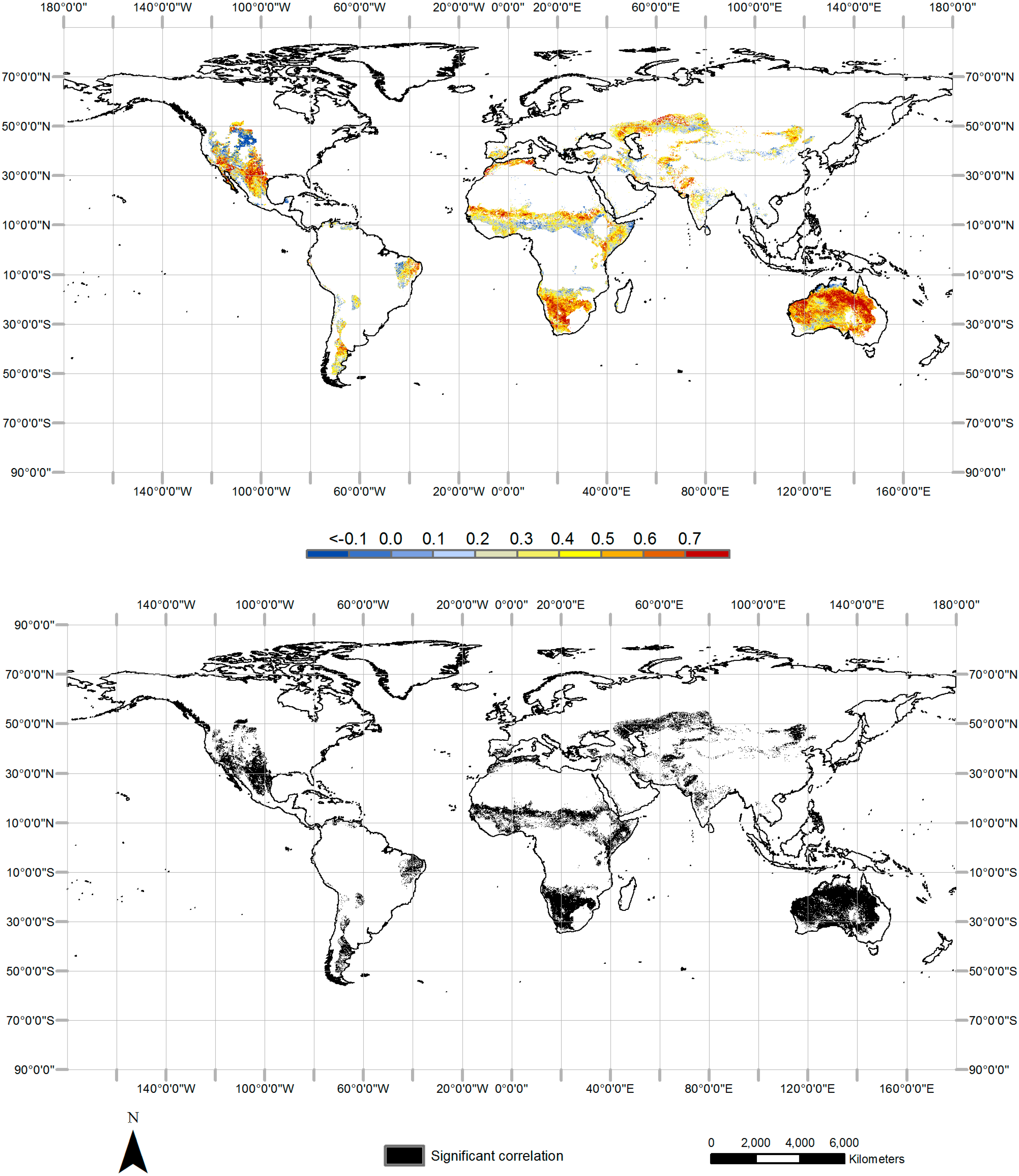
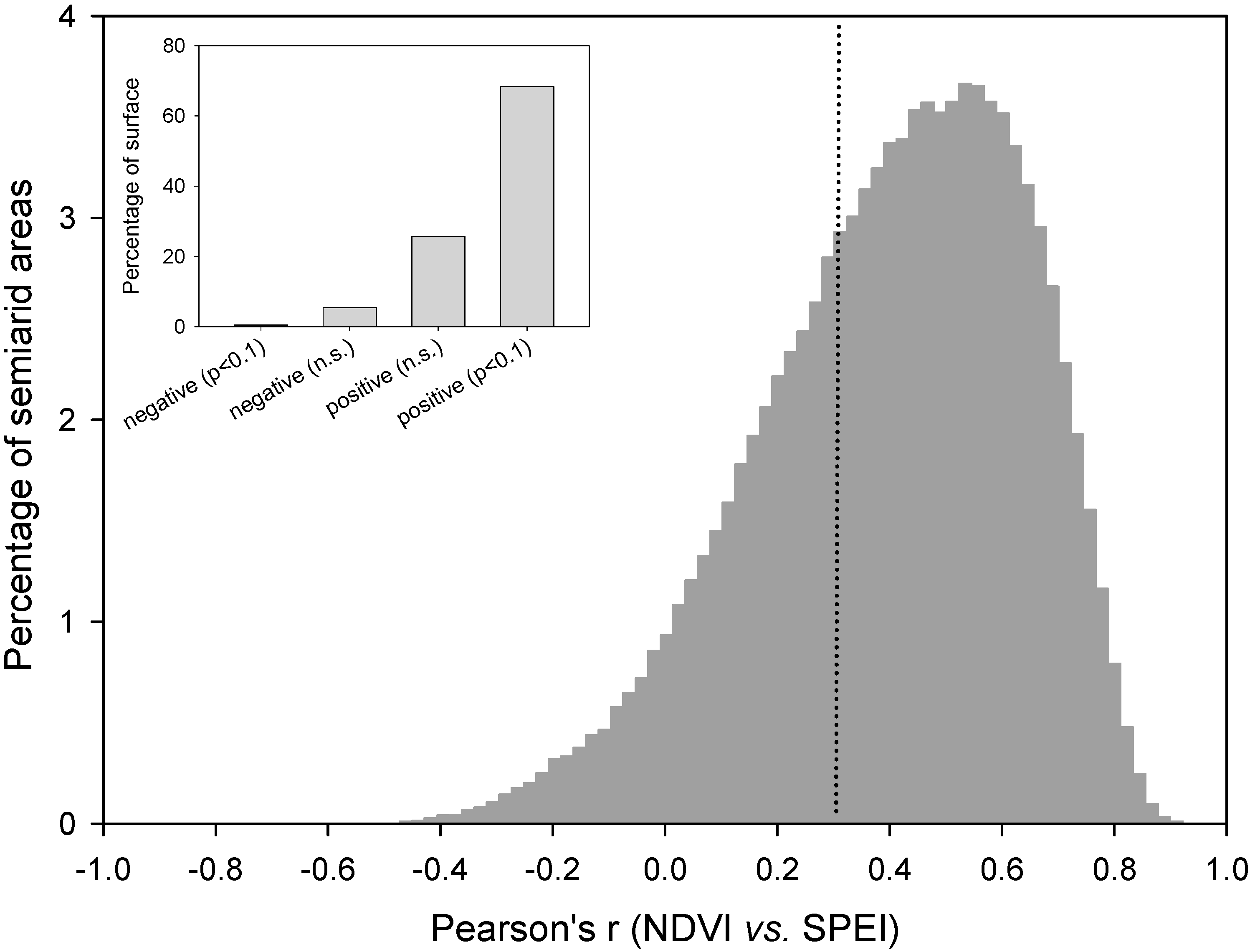
- For the majority of the world’s semiarid regions the correlation between drought and the maximum annual NDVImax was positive and statistically significant.
- There is a gradient between negative NDVImax trends, in which the magnitude of change in drought severity tends to be negative, and the positive NDVImax trends that coincide with changes toward less drought severity.
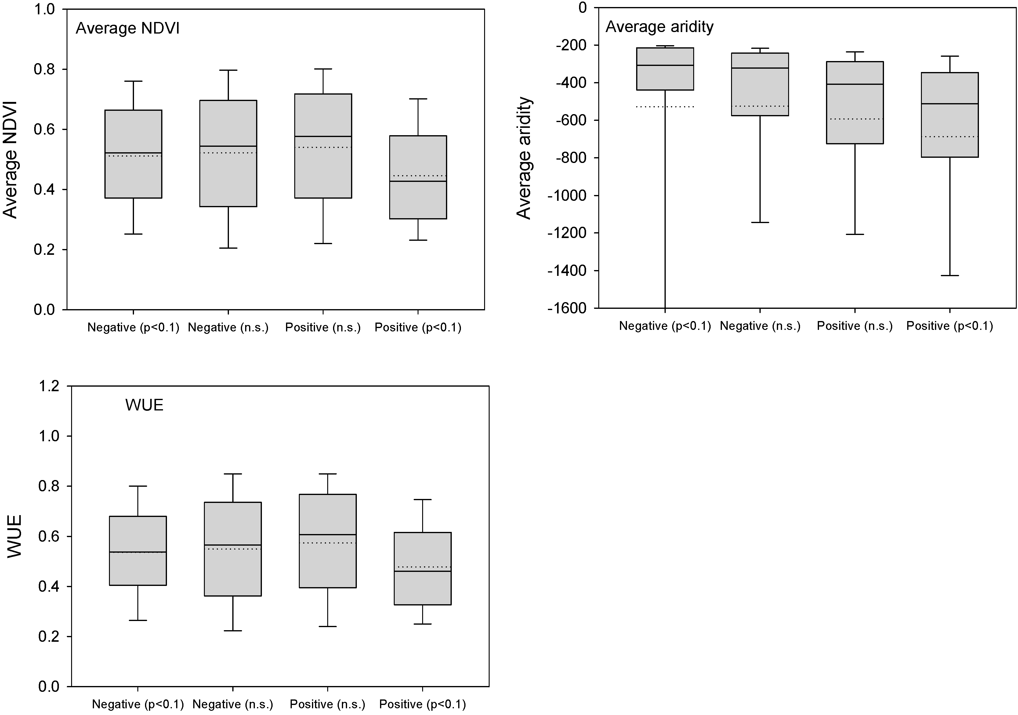
- Non-predicted NDVImax evolution based on drought severity showed predominantly positive residuals throughout semiarid regions, which means an increase in potential production much greater than expected by the evolution of drought severity, but several local and regional differences have been found.
Acknowledgments
Author Contributions
Conflicts of Interest
References
- Chaves, M.M.; Maroco, J.P.; Pereira, J.S. Understanding plant responses to drought—From genes to the whole plant. Funct. Plant. Biol. 2003, 30, 239–264. [Google Scholar]
- Le Houérou, H.N. Rain use efficiency: A unifying concept in arid-land ecology. J. Arid Environ. 1984, 7, 213–247. [Google Scholar]
- Dregne, H.E. Land degradation in the drylands. Arid Land Res. Manag. 2002, 16, 99–132. [Google Scholar] [CrossRef]
- D’Odorico, P.; Bhattachan, A.; Davis, K.F.; Ravi, S.; Runyan, C.W. Global desertification: Drivers and feedbacks. Adv. Water Resour. 2013, 51, 326–344. [Google Scholar] [CrossRef]
- Kéfi, S.; Rietkerk, M.; Alados, C.L.; Pueyo, Y.; Papanastasis, V.P.; ElAich, A.; de Ruiter, P.C. Spatial vegetation patterns and imminent desertification in Mediterranean arid ecosystems. Nature 2007, 449, 213–217. [Google Scholar] [CrossRef] [PubMed]
- Le Houérou, H.N. Climate change, drought and desertification. J. Arid Environ. 1996, 34, 133–185. [Google Scholar] [CrossRef]
- Puigdefábregas, J.; Mendizabal, T. Perspectives on desertification: Western Mediterranean. J. Arid Environ. 1998, 39, 209–224. [Google Scholar] [CrossRef]
- Barnosky, A.D.; Hadly, E.A.; Bascompte, J.; Berlow, E.L.; Brown, J.H.; Fortelius, M.; Getz, W.M.; Harte, J.; Hastings, A.; Marquet, P.A.; et al. Approaching a state shift in Earth’s biosphere. Nature 2012, 486, 52–58. [Google Scholar] [CrossRef] [PubMed]
- Trenberth, K.E. Changes in precipitation with climate change. Climate Res. 2011, 47, 123–138. [Google Scholar] [CrossRef]
- Sherwood, S.; Fu, Q. A drier future? Science 2014, 343. [Google Scholar] [CrossRef] [PubMed]
- Dai, A. Drought under global warming: A review. Wiley Interdiscip. Rev. Clim. Change 2011, 2, 45–65. [Google Scholar] [CrossRef]
- Nicholson, S.E.; Tucker, C.J.; Ba, M.B. Desertification, drought and surface vegetation: An example from the west African Sahel. Bull. Am. Meteorol. Soc. 1998, 79, 815–829. [Google Scholar] [CrossRef]
- Pickup, G. Desertification and climate change—The Australian perspective. Climate Res. 1998, 11, 51–63. [Google Scholar] [CrossRef]
- Hickler, T.; Eklundh, L.; Seaquist, J.W.; Smith, B.; Ardö, J.; Olsson, L.; Sykes, M.T.; Sjöström, M. Precipitation controls Sahel greening trend. Geophys. Res. Lett. 2005, 32. [Google Scholar] [CrossRef]
- Olsson, L.; Eklundh, L.; Ardo, J. A recent greening of the Sahel—Trends, patterns and potential causes. J. Arid Environ. 2005, 63, 556–566. [Google Scholar] [CrossRef]
- Fensholt, R.; Langanke, T.; Rasmussen, K.; Reenberg, A.; Prince, S.D.; Tucker, C.; Scholes, R.J.; Le, Q.B.; Bondeau, A.; Eastman, R.; et al. Greenness in semi-arid areas across the globe 1981–2007—An earth observing satellite based analysis of trends and drivers. Remote Sens. Environ. 2012, 121, 144–158. [Google Scholar] [CrossRef]
- Vicente-Serrano, S.M.; Zouber, A.; Lasanta, T.; Pueyo, Y. Dryness is accelerating degradation of vulnerable shrublands in semiarid Mediterranean environments. Ecol. Monogr. 2012, 82, 407–428. [Google Scholar] [CrossRef]
- Le Houérou, H.N. Man-made deserts: Desertization processes and threats. Arid Land Res. Manag. 2002, 16, 1–36. [Google Scholar] [CrossRef]
- Alados, C.L.; Puigdefábregas, J.; Martínez-Fernández, J. Ecological and socio-economical thresholds of land and plant-community degradation in semi-arid Mediterranean areas of southeastern Spain. J. Arid Environ. 2011, 75, 1368–1376. [Google Scholar] [CrossRef]
- Pueyo, Y.; Alados, C.L.; García-Ávila, B.; Kéfi, S.; Maestro, M.; Rietkerk, M. Comparing direct abiotic amelioration and facilitation as tools for restoration of semiarid grasslands. Restor. Ecol. 2009, 17, 908–916. [Google Scholar] [CrossRef]
- Narasimha-Rao, R.V.; Venkataratuam, L.; Krishna, P.V.; Ramana, K.V. Relation between root zone soil moisture and normalized difference vegetation index of vegetated fields. Int. J. Remote Sens. 1993, 14, 441–449. [Google Scholar] [CrossRef]
- Davenport, M.L.; Nicholson, S.E. On the relation between rainfall and the normalized difference vegetation index for diverse vegetation types in east Africa. Int. J. Remote Sens. 1993, 14, 2369–2389. [Google Scholar] [CrossRef]
- Xu, J.; Ren, L.-L.; Ruan, X.-H.; Liu, X.-F.; Yuan, F. Development of a physically based PDSI and its application for assessing the vegetation response to drought in northern China. J. Geophys. Res.: Atmos. 2012, 117. [Google Scholar] [CrossRef]
- Li, F.; Zhao, W.; Liu, H. The response of aboveground net primary productivity of desert vegetation to rainfall pulse in the temperate desert region of Northwest China. PLoS One 2013, 8. [Google Scholar] [CrossRef]
- Gutman, G. Towards monitoring droughts from space. J. Climate 1990, 3, 282–295. [Google Scholar] [CrossRef]
- Walsh, S.J. Comparison of NOAA-AVHRR data to meteorological drought indices. Photogramm. Eng. Remote Sens. 1987, 53, 1069–1074. [Google Scholar]
- Lotsch, A.; Friedl, M.A.; Anderson, B.T. Coupled vegetation-precipitation variability observed from satellite and climate records. Geophys. Res. Lett. 2003, 30. [Google Scholar] [CrossRef]
- Quiring, S.M.; Ganesh, S. Evaluating the utility of the Vegetation Condition Index (VCI) for monitoring meteorological drought in Texas. Agric. For. Meteorol. 2010, 150, 330–339. [Google Scholar] [CrossRef]
- Vicente-Serrano, S.M. Evaluating the impact of drought using remote sensing in a Mediterranean, semi-arid region. Nat. Hazards 2007, 40, 173–208. [Google Scholar] [CrossRef]
- Vicente-Serrano, S.M.; Gouveia, C.; Camarero, J.J.; Beguería, S.; Trigo, R.; López-Moreno, J.I.; Azorín-Molina, C.; Pasho, E.; Lorenzo-Lacruz, J.; Revuelto, J.; et al. The response of vegetation to drought time-scales across global land biomes. Proc. Natl. Acad. Sci. USA 2013, 110, 52–57. [Google Scholar] [CrossRef] [PubMed]
- Evans, J.; Geerken, R. Discrimination between climate and human-induced dryland degradation. J. Arid Environ. 2004, 57, 535–554. [Google Scholar] [CrossRef]
- Wessels, K.J.; Prince, S.D.; Malherbe, J.; Small, J.; Frost, P.E.; VanZyl, D. Can human-induced land degradation be distinguished from the effects of rainfall variability? A case study in South Africa. J. Arid Environ. 2007, 68, 271–297. [Google Scholar] [CrossRef]
- McDowell, N.; Pockman, W.T.; Allen, C.D.; Breshears, D.D.; Cobb, N.; Kolb, T.; Plaut, J.; Sperry, J.; West, A.; Williams, D.G.; et al. Mechanisms of plant survival and mortality during drought: Why do some plants survive while others succumb to drought? New Phytol. 2008, 178, 719–739. [Google Scholar] [CrossRef] [PubMed]
- De Jong, R.; de Bruin, S.; de Wit, A.; Schaepman, M.E.; Dent, D.E. Analysis of monotonic greening and browning trends from global NDVI time-series. Remote Sens. Environ. 2011, 115, 692–702. [Google Scholar] [CrossRef]
- Bai, Z.G.; Dent, D.L.; Olsson, L.; Schaepman, M.E. Proxy global assessment of land degradation. Soil Use Manag. 2008, 24, 223–234. [Google Scholar] [CrossRef]
- Verón, S.R.; Paruelo, J.M.; Oesterheld, M. Assessing desertification. J. Arid Environ. 2006, 66, 751–763. [Google Scholar] [CrossRef]
- Vicente-Serrano, S.M.; Beguería, S.; Lorenzo-Lacruz, J.; Camarero, J.J.; López-Moreno, J.I.; Azorin-Molina, C.; Revuelto, J.; Morán-Tejeda, E.; Sanchez-Lorenzo, A. Performance of drought índices for ecological, agricultural and hydrological applications. Earth Interact. 2012, 16, 1–27. [Google Scholar] [CrossRef]
- Vicente-Serrano, S.M.; Beguería, S.; López-Moreno, J.I. A Multi-scalar drought index sensitive to global warming: The Standardized Precipitation Evapotranspiration Index—SPEI. J. Climate 2010, 23, 1696–1718. [Google Scholar]
- Rouse, J.W.; Hass, R.H.; Schell, J.A.; Deering, D.W.; Harlan, J.C. Monitoring the Vernal Advancement and Retrogradation (Greenwave Effect) of Natural Vegetation; NASA/GSFC type III Final Report; GSFC: Greenbelt, MD, USA, 1974. [Google Scholar]
- Myneni, R.B.; Keeling, C.D.; Tucker, C.J.; Asrar, G.; Nemani, R.R. Increased plant growth in the northern high latitudes from 1981 to 1991. Nature 1997, 386, 698–702. [Google Scholar] [CrossRef]
- Nemani, R.R.; Keeling, C.D.; Hashimoto, H.; Jolly, W.M.; Piper, S.C.; Tucker, C.J.; Myneni, R.B.; Running, S.W. Climate-driven increases in global terrestrial net primary production from 1982 to 1999. Science 2003, 300, 1560–1563. [Google Scholar] [CrossRef] [PubMed]
- Zhou, L.; Tucker, C.J.; Kaufmann, R.K.; Slayback, D.; Shabanov, N.V.; Myneni, R.B. Variations in northern vegetation activity inferred from satellite data of vegetation index during 1981 to 1999. J. Geophys. Res.: Atmos. 2001, 106, 20069–20083. [Google Scholar] [CrossRef]
- Beck, H.E.; McVicar, T.R.; van Dijkb, A.I.J.M.; Schellekensc, J.; de Jeua, R.A.M.; Bruijnzeela, L.A. Global evaluation of four AVHRR NDVI data sets: Intercomparison and assessment against Landsat imagery. Remote Sens. Environ. 2011, 115, 2547–2563. [Google Scholar] [CrossRef]
- Tucker, C.J.; Pinzon, J.E.; Brown, M.E.; Slayback, D.A.; Pak, E.W.; Mahoney, R.; Vermote, E.F.; El Saleous, N. An extended AVHRR 8-km NDVI dataset compatible with MODIS and SPOT vegetation NDVI data. Int. J. Remote Sens. 2005, 26, 4485–4498. [Google Scholar] [CrossRef]
- Pinzon, J.E.; Tucker, C.J. A non-stationary 1981–2012 AVHRR NDVI3g time series. Remote Sens. 2014, 6, 6929–6960. [Google Scholar] [CrossRef]
- Campo-Bescós, M.A.; Muñoz-Carpena, R.; Southworth, J.; Zhu, L.; Waylen, P.R.; Bunting, E. Combined spatial and temporal effects of environmental controls on long-term monthly NDVI in the Southern Africa Savanna. Remote Sens. 2013, 5, 6513–6538. [Google Scholar] [CrossRef]
- Zeng, F-W.; Collatz, G.J.; Pinzon, J.E.; Ivanoff, A. Evaluating and quantifying the climate-driven interannual variability in Global Inventory Modeling and Mapping Studies (GIMMS) Normalized Difference Vegetation Index (NDVI3g) at global scales. Remote Sens. 2013, 5, 3918–3950. [Google Scholar] [CrossRef]
- Anyamba, A.; Small, J.L.; Tucker, C.J.; Pak, E.W. Thirty-two years of Sahelian zone growing season non-stationary NDVI3g patterns and trends. Remote Sens. 2014, 6, 3101–312. [Google Scholar] [CrossRef]
- De Jong, R.; Verbesselt, J.; Zeileis, A.; Schaepman, M.E. Shifts in global vegetation activity trends. Remote Sens. 2013, 5, 1117–1133. [Google Scholar] [CrossRef]
- Mao, J.; Shi, X.; Thornton, P.E.; Hoffman, F.M.; Zhu, Z.; Myneni, R.B. Global latitudinal-asymmetric vegetation growth trends and their driving mechanisms: 1982–2009. Remote Sens. 2013, 5, 1484–1497. [Google Scholar] [CrossRef]
- Cook, B.I.; Pau, S. A global assessment of long-term greening and browning trends in pasture lands using the GIMMS LAI3g dataset. Remote Sens. 2013, 5, 2492–2512. [Google Scholar] [CrossRef]
- Bi, J.; Xu, L.; Samanta, A.; Zhu, Z.; Myneni, R. Divergent arctic-boreal vegetation changes between north America and Eurasia over the past 30 years. Remote Sens. 2013, 5, 2093–2112. [Google Scholar] [CrossRef]
- Dardel, C.; Kergoat, L.; Hiernaux, P.; Grippa, M.; Mougin, E.; Ciais, P.; Nguyen, C.-C. Rain-use-efficiency: What it tells us about the conflicting Sahel greening and Sahelian paradox. Remote Sens. 2014, 6, 3446–3474. [Google Scholar] [CrossRef]
- Fensholt, R.; Rasmussen, K.; Kaspersen, P.; Huber, S.; Horion, S.; Swinnen, E. Assessing land degradation/recovery in the African Sahel from long-term earth observation based primary productivity and precipitation relationships. Remote Sens. 2013, 5, 664–686. [Google Scholar] [CrossRef]
- Beguería, S.; Vicente-Serrano, S.M.; Angulo, M. A multi-scalar global drought data set: The SPEIbase: A new gridded product for the analysis of drought variability and impacts. Bull. Am. Meteorol. Soc. 2010, 91, 1351–1354. [Google Scholar] [CrossRef]
- Vicente-Serrano, S.M.; Beguería, S.; López-Moreno, J.I.; Angulo, M.; El Kenawy, A. A new global 0.5° gridded dataset (1901–2006) of a multiscalar drought index: comparison with current drought index datasets based on the Palmer Drought Severity Index. J. Hydrometeorol. 2010, 11, 1033–1043. [Google Scholar] [CrossRef]
- Vicente-Serrano, S.M.; Van der Schrier, G.; Beguería, S.; Azorin-Molina, C.; Lopez-Moreno, J.I. Contribution of precipitation and reference evapotranspiration to drought indices under different climates. J. Hydrol. 2014. [Google Scholar] [CrossRef]
- Harris, I.; Jones, P.D.; Osborn, T.J.; Lister, D.H. Updated high-resolution grids of monthly climatic observations—The CRU TS3.10 dataset. Int. J. Climatol. 2014, 34, 623–642. [Google Scholar] [CrossRef]
- Köppen, W. Das geographische system der klimate. In Handbuch der Klimatologie; Köppen, C.W., Geiger, R., Eds.; Gebrüder Bornträger: Berlin, Germany, 1936; vol. 3. [Google Scholar]
- Budyko, M.I. Climate and Life; Academic: New York, NY, USA, 1974. [Google Scholar]
- UNEP. World Atlas of Desertification; Edward Arnold: London, UK, 1992. [Google Scholar]
- Holdridge, L.R. Determination of world plant formations from simple climatic data. Science 1947, 105, 367–368. [Google Scholar] [CrossRef] [PubMed]
- Kassas, M. Desertification: A general review. J. Arid Environ. 1995, 30, 115–128. [Google Scholar] [CrossRef]
- Tucker, C.J.; Vanpraet, C.; Boerwinkel, E.; Gaston, A. Satellite remote-sensing of total dry-matter production in the Senegalese Sahel. Remote Sens. Environ. 1983, 13, 461–474. [Google Scholar] [CrossRef]
- Nicholson, S.E.; Farrar, T. The influence of soil type on the relationships between NDVI, rainfall and soil moisture in semi-arid Botswana: Part I. NDVI response to rainfall. Remote Sens. Environ. 1994, 50, 107–120. [Google Scholar] [CrossRef]
- Fensholt, R.; Sandholt, I.; Rasmussen, M.S.; Stisen, S.; Diouf, A. Evaluation of satellite based primary production modelling in the semi-arid Sahel. Remote Sens. Environ. 2006, 105, 173–188. [Google Scholar] [CrossRef]
- Lanzante, J.R. Resistant, robust and non-parametric techniques for the analysis of climate data: Theory and examples including applications to historical radiosonde station data. Int. J. Climatol. 1996, 16, 1197–1226. [Google Scholar] [CrossRef]
- De Luis, M.; Vicente-Serrano, S.M.; González-Hidalgo, J.C.; Raventós, J. Aplicación de las Tablas de Contingencia (Cross Tab análisis) al análisis espacial de tendencias climáticas. Cuadernos. Investigación. Geográfica. 2003, 29, 23–34. [Google Scholar]
- Clark, W.A.V.; Hosking, P.L. Statistical Methods for Geographers; Jhon Willey & Sons: New York, NY, USA, 1986; p. 528. [Google Scholar]
- Herrmann, S.A.; Anyamba, A.; Tucker, C.J. Recent trends in vegetation dynamics in the African Sahel and their relationship to climate. Glob. Environ. Change 2005, 15, 394–404. [Google Scholar] [CrossRef]
- Fensholt, R.; Rasmussen, K. Analysis of trends in the Sahelian ‘rain-use efficiency’ using GIMMS NDVI, RFE and GPCP rainfall data. Remote Sens. Environ. 2011, 115, 438–451. [Google Scholar] [CrossRef]
- Li, A.; Wu, J.; Huang, J. Distinguishing between human-induced and climate-driven vegetation changes: A critical application of RESTREND in Inner Mongolia. Landsc. Ecol. 2012, 27, 969–982. [Google Scholar] [CrossRef]
- Prince, S.D.; De Colstoun, E.B.; Kravitz, L.L. Evidence from rain-use efficiencies does not indicate extensive Sahelian desertification. Glob. Change Biol. 1998, 4, 359–374. [Google Scholar] [CrossRef]
- Paruelo, J.M.; Lauenroth, W.K.; Burke, I.C.; Sala, E.O. Grassland precipitation-use efficiency varies across a resource gradient. Ecosystems 1999, 2, 64–68. [Google Scholar] [CrossRef]
- Illius, A.W.; O’Connor, T.G. On the relevance of nonequilibrium concepts to arid and semiarid grazing systems. Ecol. Appl. 1999, 9, 798–813. [Google Scholar] [CrossRef]
- Anyamba, A.; Tucker, C.J. Analysis of Sahelian vegetation dynamics using NOAA-AVHRR NDVI data from 1981–2003. J. Arid Environ. 2005, 63, 596–614. [Google Scholar] [CrossRef]
- Hiernaux, P.; Diarrab, L.; Trichonc, V.; Mougin, E.; Soumagueld, N.; Baupa, F. Woody plant population dynamics in response to climate changes from 1984 to 2006 in Sahel (Gourma, Mali). J. Hydrol. 2009, 375, 103–113. [Google Scholar] [CrossRef]
- Herrmann, S.M.; Tappan, G.G. Vegetation impoverishment despite greening: A case study from central Senegal. J. Arid Environ. 2013, 90, 55–66. [Google Scholar] [CrossRef]
- Schlesinger, W.H.; Reynolds, J.F.; Cunningham, G.L.; Huenneke, L.F.; Jarrell, W.M.; Virginia, R.A.; Whitford, W.G. Biological feedbacks in global desertification. Science 1990, 247, 1043–1048. [Google Scholar] [CrossRef] [PubMed]
- Reynolds, J.F.; Virginia, R.A.; Kemp, P.R.; De Soyza, A.G.; Tremmel, D.C. Impact of drought on desert shrubs: Effects of seasonality and degree of resource island development. Ecol. Monogr. 1999, 69, 69–106. [Google Scholar] [CrossRef]
- Stellmes, M.; Udelhoven, T.; Röder, A.; Sonnenschein, R.; Hill, J. Dryland observation at local and regional scale—Comparison of Landsat TM/ETM+ and NOAA AVHRR time series. Remote Sens. Environ. 2010, 114, 2111–2125. [Google Scholar] [CrossRef]
- Röder, A.; Udelhoven, T.; Hill, J.; del Barrio, G.; Tsiourlis, G. Trend analysis of Landsat-TM and ETM+ imagery to monitor grazing impact in a rangeland ecosystem in Northern Greece. Remote Sens. Environ. 2008, 112, 2863–2875. [Google Scholar] [CrossRef]
- Lasanta, T.; Vicente-Serrano, S.M. Complex land cover change processes in semiarid Mediterranean regions: An approach using Landsat images in northeast Spain. Remote Sens. Environ. 2012, 124, 1–14. [Google Scholar] [CrossRef]
- Peñuelas, J.; Gordon, C.; Llorens, L.; Nielsen, T.; Tietema, A.; Beier, C.; Bruna, P.; Emmett, B.; Estiarte, M.; Gorissen, A. Nonintrusive field experiments show different plant responses to warming and drought among sites, seasons, and species in a north-south European gradient. Ecosystems 2004, 7, 598–612. [Google Scholar] [CrossRef]
- Maselli, F.; Cherubinib, P.; Chiesia, M.; Gilabert, M.A.; Lombardie, F.; Moreno, A.; Teobaldellid, M.; Tognettie, R. Start of the dry season as a main determinant of inter-annual Mediterranean forest production variations. Agric. For. Meteorol. 2014, 194, 197–206. [Google Scholar] [CrossRef]
- Hielkema, J.U.; Prince, S.D.; Astle, W.L. Rainfall and vegetation monitoring in the savanna zone of the democratic-republic of Sudan using the NOAA advanced very high-resolution radiometer. Int. J. Remote Sens. 1986, 7, 1499–1513. [Google Scholar] [CrossRef]
- Justice, C.O.; Hiernaux, P.H.Y. Monitoring the grasslands of the Sahel using NOAA-AVHRR data. Niger, 1983. Int. J. Remote Sens. 1986, 7, 1475–1497. [Google Scholar] [CrossRef]
- Sannier, C.A.D.; Taylor, J.C. Real-time vegetation monitoring with NOAA-AVHRR in Southern Africa for wildlife management and food security assessment. Int. J. Remote Sens. 1998, 19, 621–639. [Google Scholar] [CrossRef]
- Wang, J.; Price, K.P.; Rich, P.M. Spatial patterns of NDVI response to precipitation and temperature in the central Great Plains. Int. J. Remote Sens. 2001, 22, 3827–3844. [Google Scholar] [CrossRef]
- Wessels, K.J.; Prince, S.D.; Frost, P.E.; van Zyl, D. Assessing the effects of human-induced land degradation in the former homelands of northern South Africa with a 1 km AVHRR NDVI time-series. Remote Sens. Environ. 2004, 91, 47–67. [Google Scholar] [CrossRef]
- Diouf, A.; Lambin, E.F. Monitoring land-cover changes in semi-arid regions: Remote sensing data and field observations in the Ferlo, Senegal. J. Arid Environ. 2001, 48, 129–148. [Google Scholar] [CrossRef]
- Hein, L.; de Ridder, N.; Hiernaux, P.; Leemans, R.; de Witd, A.; Schaepman, M. Desertification in the Sahel: Towards better accounting for ecosystem dynamics in the interpretation of remote sensing images. J. Arid Environ. 2011, 75, 1164–1172. [Google Scholar] [CrossRef]
- Breshears, D.D.; Adams, H.D.; Eamus, D.; McDowell, N.G.; Law, D.J.; Will, R.E.; Williams, A.P.; Zou, C.B. The critical amplifying role of increasing atmospheric moisture demand on tree mortality and associated regional die-off. Front. Plant. Sci. 2013, 4. [Google Scholar] [CrossRef]
- Anderegg, W.R.L.; Berry, J.A.; Smith, D.D.; Sperry, J.S.; Anderegg, L.D.L.; Field, C.B. The roles of hydraulic and carbon stress in a widespread climate-induced forest die-off. Proc. Natl. Acad. Sci. USA 2012, 109, 233–237. [Google Scholar] [CrossRef] [PubMed]
- Eamus, D.; Boulain, N.; Cleverly, J.; Breshears, D.D. Global change-type drought-induced tree mortality: Vapor pressure deficit is more important than temperature per se in causing decline in tree health. Ecol. Evol. 2013, 3, 2711–2729. [Google Scholar] [CrossRef] [PubMed]
- Stephenson, N.L. Climatic control of vegetation distribution: The role of the water balance. Am. Nat. 1990, 135, 649–670. [Google Scholar] [CrossRef]
- Vicente-Serrano, S.M.; Camarero, J.J.; Azorín-Molina, C. Diverse responses of forest growth to drought time-scales in the northern hemisphere. Glob. Ecol. Biogeogr. 2014, 23, 1019–1030. [Google Scholar] [CrossRef]
- Nicholson, S.E.; Davenport, M.L.; Malo, A.R. A comparison of the vegetation response to rainfall in the Sahel and east Africa, using normalized difference vegetation index from NOAA-AVHRR. Clim. Chang. 1990, 17, 209–241. [Google Scholar] [CrossRef]
- Santos, P.; Negrín, A.J. A comparison of the normalized difference vegetation index and rainfall for the Amazon and Notheastern Brazil. J. Climate 1997, 36, 958–965. [Google Scholar]
- Farrar, T.J.; Nicholson, S.E.; Lare, A.R. The influence of soil type on the relationships between NDVI, rainfall and soil moisture in semiarid Botswana II: NDVI response to soil moisture. Remote Sens. Environ. 1994, 50, 121–133. [Google Scholar] [CrossRef]
- Donohue, R.J.; Roderick, M.L.; McVicar, T.R.; Farquhar, G.D. Impact of CO2 fertilization on maximum foliage cover across the globe’s warm, arid environments. Geophys. Res. Lett. 2013, 40, 3031–3035. [Google Scholar] [CrossRef]
- Farquhar, G.D. Carbon dioxide and vegetation. Science 1997, 278. [Google Scholar] [CrossRef] [PubMed]
- Higgins, S.I.; Scheiter, S. Atmospheric CO2 forces abrupt vegetation shifts locally, but not globally. Nature 2012, 488, 209–212. [Google Scholar] [CrossRef] [PubMed]
- Smith, S.D.; Huxman, T.E.; Zitzer, S.F.; Charlet, T.N.; Housman, D.C.; Coleman, J.S.; Fenstermaker, L.K.; Seemann, J.R.; Nowak, R.S. Elevated CO2 increases productivity and invasive species success in an arid ecosystem. Nature 2000, 408, 79–82. [Google Scholar] [CrossRef] [PubMed]
- Reich, P.B.; Hobbie, S.A.; Lee, T.D. Plant growth enhancement by elevated CO2 eliminated by joint water and nitrogen limitation. Nature Geosci. 2014, 7, 920–924. [Google Scholar] [CrossRef]
- Begue, A.; Vintrou, E.; Ruelland, D.; Claden, M.; Dessay, N. Can a 25-year trend in Soudano-Sahelian vegetation dynamics be interpreted in terms of land use change? A remote sensing approach. Glob. Environ. Change 2011, 21, 413–420. [Google Scholar] [CrossRef]
- Brink, A.B.; Eva, H.D. Monitoring 25 years of land cover change dynamics in Africa: A sample based remote sensing approach. Appl. Geogr. 2009, 29, 501–512. [Google Scholar] [CrossRef]
- Reij, C.; Tappan, G.; Belemvire, A. Changing land management practices and vegetation on the Central Plateau of Burkina Faso (1968–2002). J. Arid Environ. 2005, 63, 642–659. [Google Scholar] [CrossRef]
- Rasmussen, K.; Fog, B.; Madsen, J.E. Desertification in reverse? Observations from northern Burkina Faso. Glob. Environ. Change 2001, 11, 271–282. [Google Scholar] [CrossRef]
- Van Auken, O.W. Shrub invasions of North American Semiarid grasslands. Annu. Rev. Ecol. Syst. 2000, 31, 197–215. [Google Scholar] [CrossRef]
© 2015 by the authors; licensee MDPI, Basel, Switzerland. This article is an open access article distributed under the terms and conditions of the Creative Commons Attribution license (http://creativecommons.org/licenses/by/4.0/).
Share and Cite
Vicente-Serrano, S.M.; Cabello, D.; Tomás-Burguera, M.; Martín-Hernández, N.; Beguería, S.; Azorin-Molina, C.; Kenawy, A.E. Drought Variability and Land Degradation in Semiarid Regions: Assessment Using Remote Sensing Data and Drought Indices (1982–2011). Remote Sens. 2015, 7, 4391-4423. https://doi.org/10.3390/rs70404391
Vicente-Serrano SM, Cabello D, Tomás-Burguera M, Martín-Hernández N, Beguería S, Azorin-Molina C, Kenawy AE. Drought Variability and Land Degradation in Semiarid Regions: Assessment Using Remote Sensing Data and Drought Indices (1982–2011). Remote Sensing. 2015; 7(4):4391-4423. https://doi.org/10.3390/rs70404391
Chicago/Turabian StyleVicente-Serrano, Sergio M., Daniel Cabello, Miquel Tomás-Burguera, Natalia Martín-Hernández, Santiago Beguería, Cesar Azorin-Molina, and Ahmed El Kenawy. 2015. "Drought Variability and Land Degradation in Semiarid Regions: Assessment Using Remote Sensing Data and Drought Indices (1982–2011)" Remote Sensing 7, no. 4: 4391-4423. https://doi.org/10.3390/rs70404391
APA StyleVicente-Serrano, S. M., Cabello, D., Tomás-Burguera, M., Martín-Hernández, N., Beguería, S., Azorin-Molina, C., & Kenawy, A. E. (2015). Drought Variability and Land Degradation in Semiarid Regions: Assessment Using Remote Sensing Data and Drought Indices (1982–2011). Remote Sensing, 7(4), 4391-4423. https://doi.org/10.3390/rs70404391