
Satellite Images for Monitoring Mangrove Cover Changes in a Fast Growing Economic Region in Southern Peninsular Malaysia


 ,
,
Abstract
:
1. Introduction

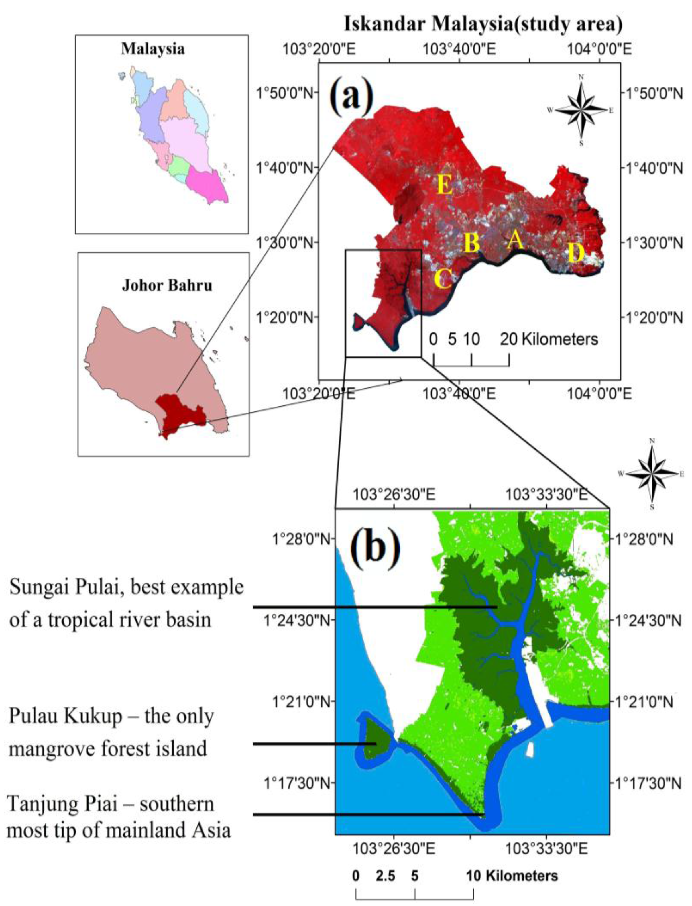
2. Study Area
3. Data and Methodology

| Landsat Images | Cloud Coverage (%) | Brightness Temperature (°C) |
|---|---|---|
| 13 September 1989 | 6 | <16 |
| 28 April 2000 | 10 | <17 |
| 4 May 2005 | 2 | <16 |
| 10 May 2007 | 5 | <17 |
| 8 February 2009 | 0 | - |
| 27 June 2013 | 10 | <18 |
| 13 May 2014 | 20 | <18 |

4. Results
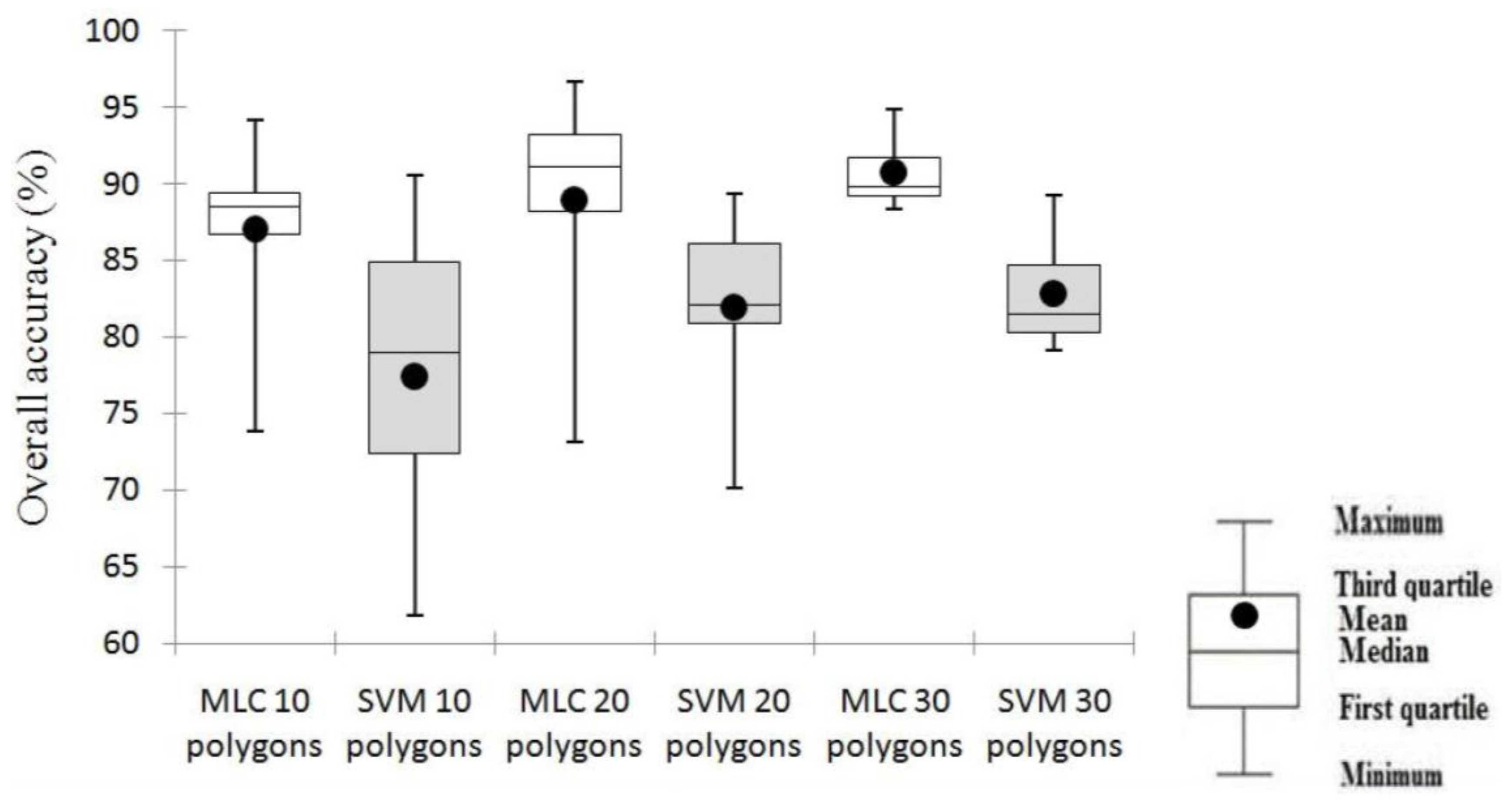
4.1. Classification Accuracy
| Year | Classification | Sample Size (Polygons) | Forest | Oil Palm | Rubber | Mangrove | Urban | Water Body | Overall Accuracies | |||||||
|---|---|---|---|---|---|---|---|---|---|---|---|---|---|---|---|---|
| PA (%) | UA (%) | PA (%) | UA (%) | PA (%) | UA (%) | PA (%) | UA (%) | PA (%) | UA (%) | PA (%) | UA (%) | OA (%) | Kappa | |||
| 1989 | SVM R | 10 | 68.71 | 90.10 | 47.49 | 43.18 | 76.03 | 85.96 | 90.76 | 96.13 | 53.94 | 40.54 | 98.25 | 86.36 | 71.51 | 0.65 |
| 1989 | MLC | 10 | 74.09 | 96.82 | 36.14 | 57.55 | 82.79 | 98.45 | 95.34 | 75.75 | 66.95 | 40.33 | 97.98 | 100.00 | 73.86 | 0.70 |
| 1989 | SVM R | 20 | 60.59 | 93.86 | 45.54 | 41.14 | 77.34 | 83.73 | 92.48 | 92.61 | 57.64 | 40.28 | 98.38 | 86.89 | 70.09 | 0.63 |
| 1989 | MLC | 20 | 77.67 | 96.96 | 44.89 | 42.23 | 75.82 | 8.86 | 82.31 | 99.05 | 67.18 | 39.43 | 98.11 | 100.00 | 73.10 | 0.67 |
| 1989 | SVMR | 30 | 53.54 | 97.50 | 83.69 | 54.97 | 79.31 | 71.32 | 98.32 | 99.25 | 96.20 | 99.56 | 100.00 | 97.22 | 81.53 | 0.77 |
| 1989 | MLC | 30 | 67.30 | 66.20 | 74.46 | 90.03 | 99.43 | 85.86 | 100.00 | 94.88 | 100.00 | 92.76 | 100.00 | 100.00 | 89.22 | 0.85 |
| 2000 | SVM R | 10 | 84.01 | 96.71 | 99.76 | 62.83 | 1.53 | 10.29 | 99.07 | 99.78 | 85.38 | 100.00 | 100.00 | 100.00 | 86.54 | 0.83 |
| 2000 | MLC | 10 | 90.74 | 98.96 | 99.20 | 78.54 | 58.82 | 97.83 | 99.86 | 99.08 | 97.08 | 100.00 | 100.00 | 100.00 | 94.07 | 0.93 |
| 2000 | SVM R | 20 | 84.45 | 96.80 | 99.28 | 72.06 | 54.68 | 49.70 | 99.57 | 99.29 | 62.46 | 100.00 | 100.00 | 99.87 | 87.43 | 0.84 |
| 2000 | MLC | 20 | 91.81 | 99.18 | 98.72 | 81.47 | 71.68 | 98.21 | 99.86 | 99.22 | 96.26 | 100.00 | 100.00 | 100.00 | 95.08 | 0.94 |
| 2000 | SVMR | 30 | 95.74 | 34.13 | 100.00 | 30.26 | 65.77 | 80.10 | 87.78 | 99.96 | 72.84 | 98.29 | 98.86 | 99.83 | 83.50 | 0.79 |
| 2000 | MLC | 30 | 89.85 | 84.84 | 93.22 | 87.21 | 83.94 | 92.42 | 87.85 | 87.60 | 75.51 | 95.84 | 98.15 | 99.00 | 89.83 | 0.86 |
| 2005 | SVM R | 10 | 83.95 | 96.36 | 98.24 | 59.96 | 0.00 | 0.00 | 99.64 | 93.42 | 72.73 | 100.00 | 99.73 | 100.00 | 85.11 | 0.82 |
| 2005 | MLC | 10 | 78.51 | 93.28 | 91.98 | 71.15 | 55.77 | 89.51 | 96.06 | 98.31 | 99.18 | 91.97 | 97.44 | 94.64 | 88.49 | 0.86 |
| 2005 | SVM R | 20 | 70.69 | 98.50 | 99.28 | 65.16 | 46.84 | 96.85 | 99.00 | 93.13 | 92.61 | 100.00 | 100.00 | 99.73 | 87.35 | 0.84 |
| 2005 | MLC | 20 | 65.80 | 95.22 | 98.56 | 68.51 | 78.00 | 97.81 | 99.57 | 97.89 | 99.76 | 98.44 | 99.73 | 100.00 | 89.31 | 0.87 |
| 2005 | SVMR | 30 | 83.32 | 57.58 | 79.65 | 83.30 | 84.64 | 80.49 | 73.89 | 100.00 | 100.00 | 99.84 | 100.00 | 97.72 | 85.88 | 0.82 |
| 2005 | MLC | 30 | 96.51 | 68.42 | 87.74 | 98.04 | 98.21 | 65.77 | 94.68 | 98.35 | 100.00 | 99.40 | 99.66 | 100.00 | 92.42 | 0.89 |
| 2007 | SVM R | 10 | 80.23 | 48.08 | 95.75 | 55.79 | 0.00 | 0.00 | 4.15 | 61.70 | 72.75 | 96.28 | 99.46 | 96.22 | 61.77 | 0.52 |
| 2007 | MLC | 10 | 77.62 | 94.36 | 94.39 | 71.33 | 57.52 | 91.03 | 95.85 | 98.24 | 99.06 | 92.37 | 97.44 | 95.26 | 88.81 | 0.86 |
| 2007 | SVM R | 20 | 64.69 | 96.86 | 97.91 | 56.95 | 0.00 | 0.00 | 96.92 | 92.10 | 78.83 | 97.54 | 99.73 | 92.28 | 79.82 | 0.75 |
| 2007 | MLC | 20 | 80.99 | 95.72 | 93.99 | 80.77 | 79.08 | 91.21 | 95.20 | 97.36 | 99.53 | 90.92 | 97.31 | 91.29 | 91.06 | 0.89 |
| 2007 | SVMR | 30 | 45.26 | 96.09 | 74.25 | 75.02 | 73.47 | 51.22 | 98.30 | 92.02 | 84.93 | 77.50 | 98.63 | 100.00 | 79.63 | 0.74 |
| 2007 | MLC | 30 | 67.20 | 90.07 | 89.20 | 87.82 | 88.63 | 88.37 | 94.18 | 93.13 | 87.16 | 70.70 | 98.54 | 100.00 | 89.26 | 0.86 |
| 2009 | SVM R | 10 | 71.76 | 94.57 | 86.37 | 63.32 | 54.25 | 60.73 | 95.70 | 100.00 | 90.29 | 93.01 | 100.00 | 92.53 | 84.58 | 0.81 |
| 2009 | MLC | 10 | 85.47 | 96.98 | 91.82 | 72.15 | 48.15 | 97.79 | 96.28 | 100.00 | 100.00 | 90.76 | 99.46 | 93.78 | 90.04 | 0.88 |
| 2009 | SVM R | 20 | 63.58 | 96.72 | 90.14 | 58.33 | 53.16 | 61.31 | 95.70 | 98.60 | 82.46 | 93.25 | 100.00 | 92.41 | 82.12 | 0.78 |
| 2009 | MLC | 20 | 94.54 | 92.37 | 83.96 | 88.43 | 88.02 | 98.54 | 95.56 | 99.85 | 100.00 | 87.60 | 99.60 | 97.75 | 93.53 | 0.92 |
| 2009 | SVMR | 30 | 81.51 | 96.89 | 98.77 | 74.86 | 47.79 | 85.81 | 93.81 | 99.45 | 99.82 | 99.72 | 99.96 | 100.00 | 88.62 | 0.84 |
| 2009 | MLC | 30 | 88.95 | 94.43 | 94.31 | 92.34 | 97.61 | 100.00 | 98.24 | 94.62 | 85.22 | 86.61 | 99.84 | 99.84 | 94.61 | 0.93 |
| 2013 | SVM R | 10 | 31.81 | 87.42 | 87.95 | 56.81 | 9.80 | 90.00 | 98.42 | 67.06 | 90.88 | 94.07 | 97.01 | 99.20 | 73.14 | 0.67 |
| 2013 | MLC | 10 | 83.71 | 78.76 | 79.54 | 84.72 | 47.06 | 96.43 | 98.42 | 87.13 | 98.36 | 83.85 | 83.33 | 100.00 | 85.67 | 0.82 |
| 2013 | SVM R | 20 | 71.06 | 91.51 | 88.22 | 65.23 | 38.34 | 87.56 | 99.86 | 87.78 | 90.99 | 95.23 | 98.27 | 99.21 | 84.75 | 0.81 |
| 2013 | MLC | 20 | 95.66 | 87.88 | 85.30 | 89.58 | 68.85 | 99.68 | 100.00 | 98.59 | 99.30 | 89.37 | 94.65 | 99.83 | 92.97 | 0.91 |
| 2013 | SVMR | 30 | 81.51 | 96.89 | 98.77 | 74.86 | 47.79 | 85.81 | 93.81 | 99.45 | 99.82 | 99.72 | 99.96 | 100.00 | 80.98 | 0.75 |
| 2013 | MLC | 30 | 75.23 | 87.23 | 98.77 | 74.86 | 100.00 | 96.89 | 93.27 | 95.04 | 83.02 | 79.12 | 89.32 | 100.00 | 91.02 | 0.88 |
| 2014 | SVM R | 10 | 74.03 | 86.66 | 63.95 | 77.49 | 70.37 | 36.41 | 99.71 | 84.36 | 60.94 | 88.76 | 97.85 | 100.00 | 79.00 | 0.74 |
| 2014 | MLC | 10 | 78.54 | 97.64 | 80.60 | 91.77 | 93.46 | 96.40 | 99.71 | 86.46 | 98.71 | 68.51 | 77.66 | 100.00 | 87.80 | 0.85 |
| 2014 | SVM R | 20 | 72.91 | 85.20 | 85.73 | 64.05 | 26.36 | 99.18 | 99.93 | 83.23 | 79.06 | 87.91 | 97.04 | 100.00 | 81.88 | 0.78 |
| 2014 | MLC | 20 | 75.16 | 97.89 | 86.83 | 79.02 | 80.61 | 99.73 | 99.86 | 87.07 | 96.14 | 74.32 | 80.35 | 100.00 | 87.15 | 0.84 |
| 2014 | SVMR | 30 | 78.47 | 88.89 | 67.70 | 94.87 | 69.63 | 8.43 | 96.74 | 97.78 | 99.80 | 97.21 | 100.00 | 99.87 | 79.17 | 0.71 |
| 2014 | MLC | 30 | 85.88 | 100.00 | 86.70 | 87.17 | 92.31 | 81.08 | 86.15 | 96.55 | 94.64 | 77.37 | 85.42 | 100.00 | 88.37 | 0.85 |

| Land Use Types | MLC 1989 (ha) | Land Use (DOA) 1990 (ha) | RPE (%) | MLC 2000 (ha) | Land Use (DOA) 2000 (ha) | RPE (%) | MLC 2005 (ha) | CDP 2005 (ha) | RPE (%) | MLC 2009 (ha) | Land Use (DOA) 2010 (ha) | RPE (%) |
| Forest | 19,396 | 17,872 | 9 | 19,186 | 15,620 | 16 | 6720 | 6879 | −1 | 6829 | 6612 | 3 |
| Oil Palm | 82,452 | 77,343 | 7 | 114,139 | 113,110 | 2 | 117,715 | / | / | 117,826 | 120,879 | −3 |
| Mangrove | 18,403 | 17,046 | 8 | 15,066 | 17,460 | −24 | 13,977 | 13,498 | 5 | 13,942 | 12,608 | 11 |
| Urban | 29,728 | 30,112 | −2 | 37,201 | 36,360 | 3 | 51,294 | / | / | 53,306 | 52,998 | 1 |
| Rubber | 46,443 | 50,559 | −9 | 9,272 | 12,450 | −6 | 2768 | / | / | 4629 | 3291 | 41 |
| Water | 13,203 | 15,099 | −13 | 13,099 | 13,000 | 1 | 12,571 | 12,401 | 1 | 11,471 | 11,046 | 4 |
| Forest + Mangrove | 37,799 | 34,918 | 1 | 34,252 | 33,091 | 3 | 20,697 | 20,377 | 1 | 20,753 | 19,220 | 8 |
| Oil palm + Rubber | 128,895 | 127,902 | 9 | 123,411 | 125,573 | −2 | 120,483 | 119,302 | 1 | 122,455 | 124,170 | −1 |
| MLC 2013 (ha) | CDP 2012 (ha) | RPE (%) | MLC 2014 (ha) | CDP 2012 (ha) | RPE (%) | |||||||
| Forest | 6829 | 6879 | −1 | 6828 | 6879 | −1 | ||||||
| Oil Palm | 115,042 | / | / | 114,744 | / | / | ||||||
| Mangrove | 12,434 | 12,606 | −1 | 12,733 | 12,606 | −1 | ||||||
| Urban | 60,110 | 56,138 | 7 | 60,354 | 56,138 | 8 | ||||||
| Rubber | 1661 | / | / | 2043 | / | / | ||||||
| Water | 12,050 | 37,234 | −68 | 11,467 | 37,234 | −69 | ||||||
| Forest + Mangrove | 19,263 | 19,485 | −1 | 19,132 | 19,485 | −2 | ||||||
| Oil palm + Rubber | 116,703 | 95,508 | 22 | 116,787 | 95,508 | 22 |

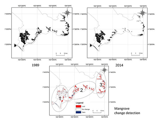
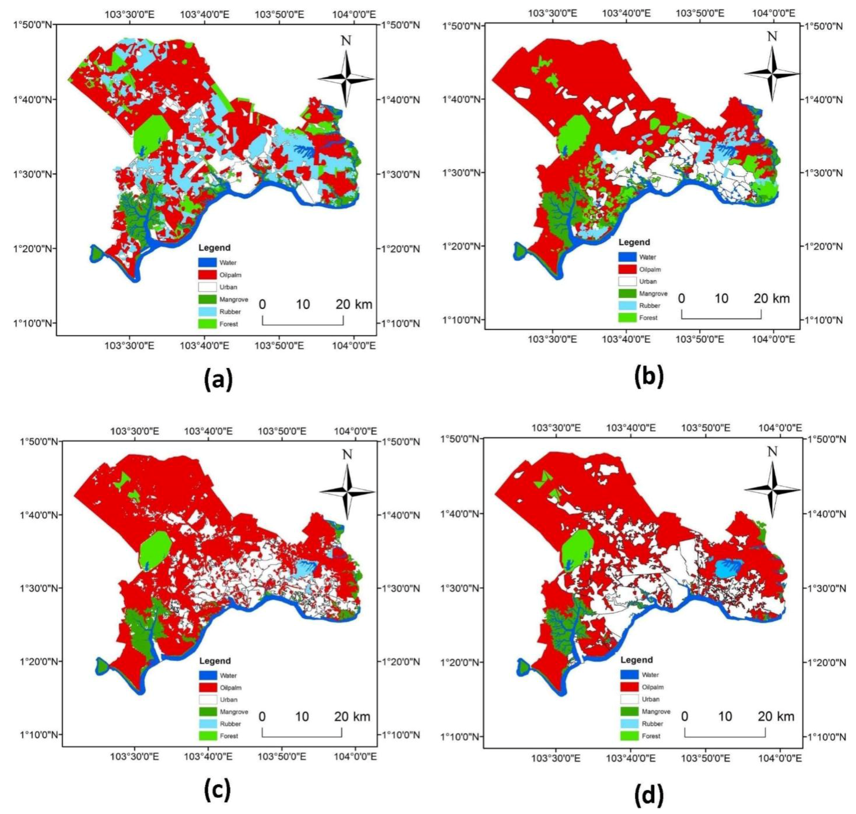
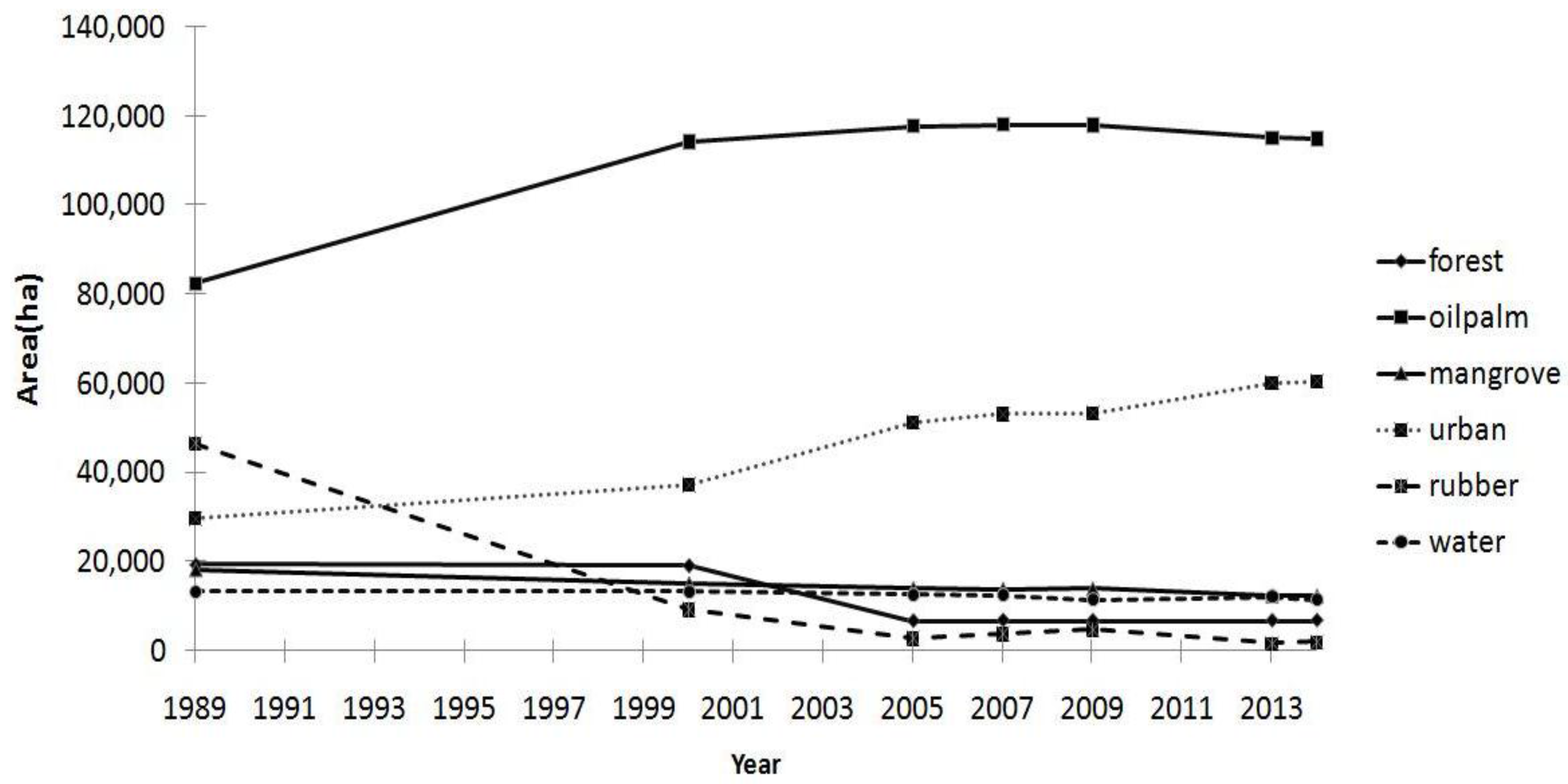
4.2. Land Use or Land Cover (LULC) Changes
| Land Use | 1989 | 2000 | 2005 | 2007 | 2009 | 2013 | 2014 |
|---|---|---|---|---|---|---|---|
| Forest | 0 | −1 | −65 | −65 | −65 | −65 | −65 |
| Oil Palm | 0 | 38 | 43 | 43 | 43 | 40 | 43 |
| Mangrove | 0 | −18 | −24 | −25 | −24 | −32 | −33 |
| Urban | 0 | 25 | 73 | 78 | 79 | 102 | 103 |
| Rubber | 0 | −80 | −94 | −92 | −90 | −96 | −96 |
| Water | 0 | −1 | −5 | −6 | −13 | −9 | −13 |
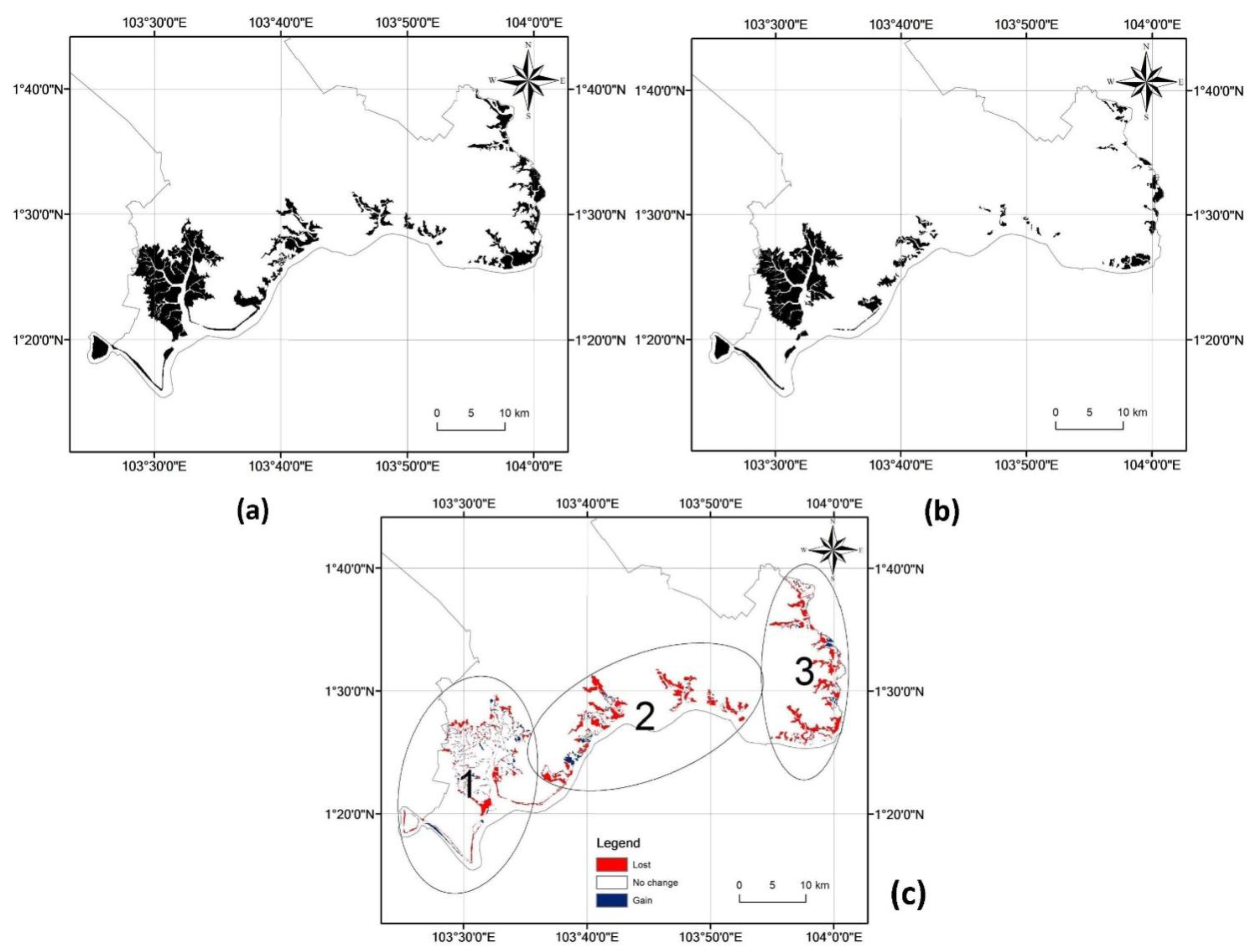
| Areas | Location |
|---|---|
| 1 | The three Ramsar (Tanjung Piai, Pulau Kukup, and Sungai Pulai) sites that cover 647 ha, 526 ha and 9126 ha of mangroves respectively |
| 2 | Pendas Forest and along Pendas, Perepat, Melayu, Skudai, Danga, and Tebrau rivers, Nusajaya, Horizon Hills, Permas Jaya, Masai and Johor Bahru City |
| 3 | Along Johor, Serai, and Kong Kong rivers, Pasir Gudang Port and Tanjung Langsat Industrial Area |

| Point | Place Name/Locations | Lat Long | Areas Corresponding to Figure 7 | Change of Land Use |
|---|---|---|---|---|
| 1 | ATT Terminal Bin | 1°20′40.47′′N 103°31′47.13′′E | 1 | mangrove to industrial |
| 2 | Nusajaya | 1°23′0.21′′N 103°36′43.95′′E | 1 | still mangrove |
| 3 | Nusajaya | 1°27′27.41′′N 103°40′37.35′′E | 2 | mangrove to oil palm |
| 4 | Taman Laguna | 1°27′57.45′′N 103°42′18.15′′E | 2 | mangrove to residential |
| 5 | Kampung Tuah Jaya | 1°28′30.24′′N 103°40′50.00′′E | 2 | mangrove to residential |
| 6 | Taman Tampoi Indah | 1°30′40.12′′N 103°40′40.73′′E | 2 | mangrove to residential |
| 7 | Taman Perindustrian JB Perdana | 1°30′1.50′′N 103°40′2.86′′E | 2 | mangrove to industrial |
| 8 | Taman Perumahan Rakyat Sri Stulang | 1°29′43.16′′N 103°47′18.78′′E | 2 | mangrove to residential |
| 9 | Kampung Sri Tasek | 1°30′23.92′′N 103°47′27.59′′E | 2 | mangrove to residential |
| 10 | Senibong Cove | 1°29′0.07′′N 103°50′12.42′′E | 2 | mangrove to residential |
| 11 | Kampung Rekoh | 1°28′39.02′′N 103°51′28.46′′E | 2 | mangrove to vacant land |
| 12 | Kampung Sri Aman | 1°26′52.46′′N 103°58′18.78′′E | 3 | mangrove to ponds |
| 13 | Tanjung Langsat | 1°27′7.49′′N 104° 0′14.23′′E | 3 | mangrove to industrial |
| 14 | Kampung Kong Kong | 1°30′41.71′′N 103°59′0.65′′E | 3 | mangrove to ponds |
| 15 | Hutan Rizab Sg Johor | 1°33′8.61′′N 103°59′49.73′′E | 3 | mangrove to agricultural land |
| 16 | Hutan Rizab Sg Johor | 1°34′10.21′′N 103°59′8.26′′E | 3 | mangrove to vacant land |
| 17 | Jova Resort Sdn Bhd | 1°35′23.08′′N 103°57′26.75′′E | 3 | mangrove to ponds |
| 18 | Nam Heng Estate | 1°37′1.07′′N 103°57′6.64′′E | 3 | mangrove to oil palm |
5. Discussion
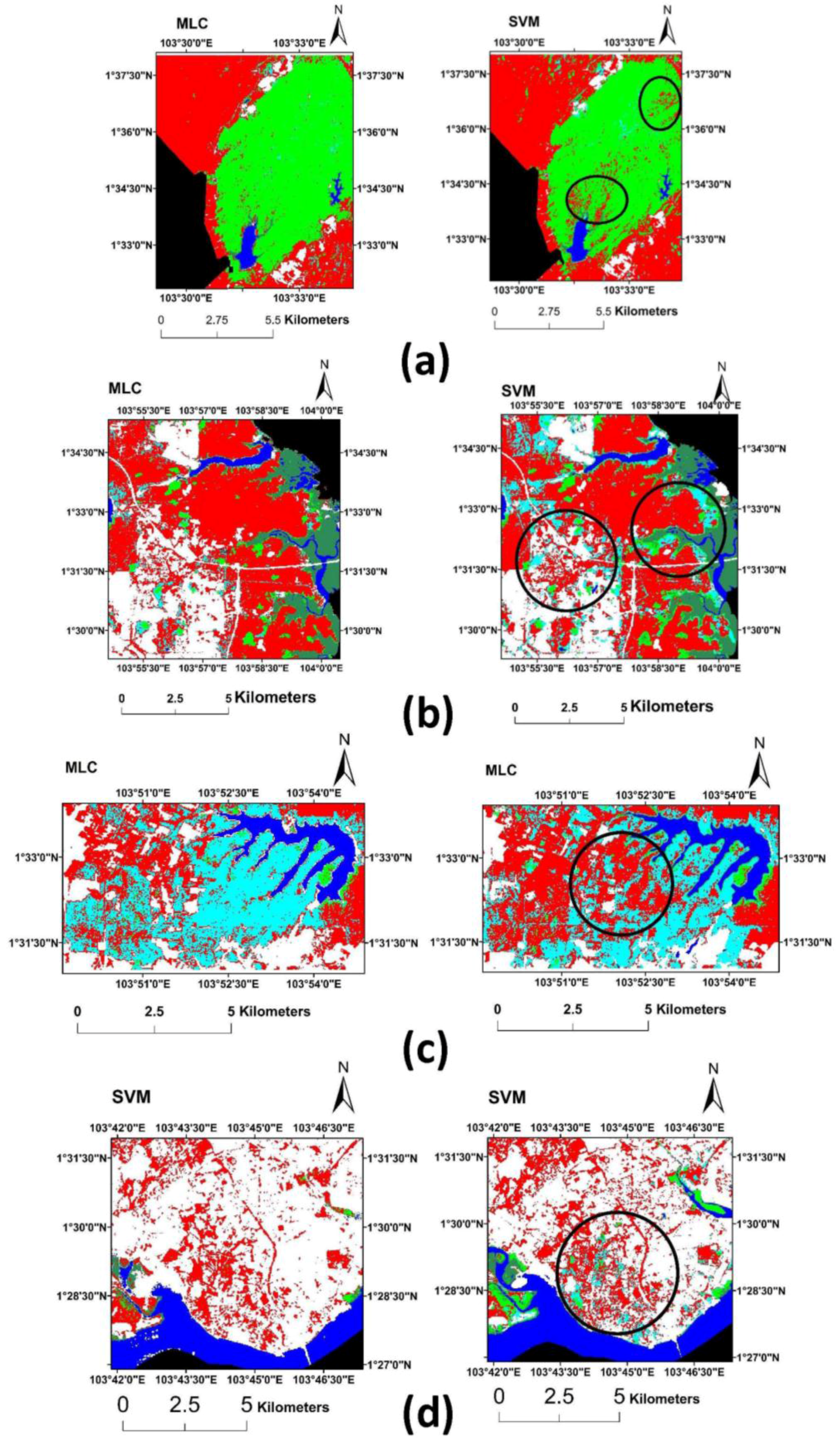
5.1. The Choice of Image Classification Algorithms
5.2. Mangrove Cover Change
6. Conclusions
Acknowledgments
Author Contributions
Conflicts of Interest
References
- Giri, C.; Ochieng, E.; Tieszen, L.L.; Zhu, Z.; Singh, A.; Loveland, T.; Masek, J.; Duke, N. Status and distribution of mangrove forests of the world using earth observation satellite data. Glob. Ecol. Biogeogr. 2011, 20, 154–159. [Google Scholar] [CrossRef]
- Spalding, M.; Kainuma, M.; Collins, L. World Atlas of Mangroves, 2nd ed.; Earthscan: London, UK, 2010; p. 350. [Google Scholar]
- Dittmar, T.; Hertkorn, N.; Kattner, G.; Lara, R.J. Mangroves, a major source of dissolved organic carbon to the oceans. Glob. Biogeochem. Cycle 2006, 20. [Google Scholar] [CrossRef]
- Donato, D.C.; Kauffman, J.B.; Murdiyarso, D.; Kurnianto, S.; Stidham, M.; Kanninen, M. Mangroves among the most carbon-rich forests in the tropics. Nat. Geosci. 2011, 4, 293–297. [Google Scholar] [CrossRef]
- Hamdan, O.; Aziz, H.K.; Hasmadi, I.M. L-band ALOS PALSAR for biomass estimation of Matang mangroves, Malaysia. Remote Sens. Environ. 2014, 155, 69–78. [Google Scholar] [CrossRef]
- Cornforth, W.A.; Fatoyinbo, T.E.; Freemantle, T.P.; Pettorelli, N. Advanced land observing satellite phased array type L-band SAR (ALOS PALSAR) to inform the conservation of mangroves: Sundarbans as a case study. Remote Sens. 2013, 5, 224–237. [Google Scholar] [CrossRef]
- Mubarak, H.T.; Azian, M. Mangroves ecosystem. In Status of Mangroves in Peninsular Malaysia; Omar, M., Aziz, K., Shamsudin, I., Raja Barizian, R.S., Eds.; Forest Research Institute Malaysia: Kuala Lumpur, Malaysia, 2012; pp. 11–30. [Google Scholar]
- FAO. The World’s Mangroves 1980–2005. A Thematic Study Prepared in the Framework of the Global Forest Resources Assessment 2005; UN FAO: Rome, Italy, 2007; p. 153. [Google Scholar]
- Omar, H. Mangroves threats and changes. In Status of Mangroves in Peninsular Malaysia; Omar, M., Aziz, K., Shamsudin, I., Raja Barizian, R.S., Eds.; Forest Research Institute Malaysia: Kuala Lumpur, Malaysia, 2012; pp. 89–110. [Google Scholar]
- Polidoro, B.A.; Carpenter, K.E.; Collins, L.; Duke, N.C.; Ellison, A.M.; Ellison, J.C.; Farnsworth, E.J.; Fernando, E.S.; Kathiresan, K.; Koedam, N.E. The loss of species: Mangrove extinction risk and geographic areas of global concern. PLoS ONE 2010, 5. [Google Scholar] [CrossRef] [PubMed]
- Kuenzer, C.; Bluemel, A.; Gebhardt, S.; Quoc, T.V.; Dech, S. Remote sensing of mangrove ecosystems: A review. Remote Sens. 2011, 3, 878–928. [Google Scholar] [CrossRef]
- Azian, M.; Mubarak, H.T. Functions and values of mangroves. In Status of Mangroves in Peninsular Malaysia; Omar, M., Aziz, K., Shamsudin, I., Raja Barizian, R.S., Eds.; Forest Research Institute Malaysia: Kuala Lumpur, Malaysia, 2012; pp. 12–25. [Google Scholar]
- Benfield, S.L.; Guzman, H.M.; Mair, J.M. Temporal mangrove dynamics in relation to coastal development in Pacific Panama. J. Environ. Manag. 2005, 76, 263–276. [Google Scholar] [CrossRef] [PubMed]
- Manson, F.; Loneragan, N.; Phinn, S. Spatial and temporal variation in distribution of mangroves in Moreton bay, subtropical Australia: A comparison of pattern metrics and change detection analyses based on aerial photographs. Estuar. Coast. Shelf Sci. 2003, 57, 653–666. [Google Scholar] [CrossRef]
- Fromard, F.; Vega, C.; Proisy, C. Half a century of dynamic coastal change affecting mangrove shorelines of French Guiana. A case study based on remote sensing data analyses and field surveys. Mar. Geol. 2004, 208, 265–280. [Google Scholar] [CrossRef]
- Giri, C.; Long, J.; Abbas, S.; Murali, R.M.; Qamer, F.M.; Pengra, B.; Thau, D. Distribution and dynamics of mangrove forests of South Asia. J. Environ. Manag. 2015, 148, 101–111. [Google Scholar] [CrossRef] [PubMed]
- Kamal, M.; Phinn, S. Hyperspectral data for mangrove species mapping: A comparison of pixel-based and object-based approach. Remote Sens. 2011, 3, 2222–2242. [Google Scholar] [CrossRef]
- Sulong, I.; Mohd-Lokman, H.; Mohd-Tarmizi, K.; Ismail, A. Mangrove mapping using Landsat imagery and aerial photographs: Kemaman district, Terengganu, Malaysia. Environ. Dev. Sustain. 2002, 4, 135–152. [Google Scholar] [CrossRef]
- Satyanarayana, B.; Mohamad, K.A.; Idris, I.F.; Husain, M.-L.; Dahdouh-Guebas, F. Assessment of mangrove vegetation based on remote sensing and ground-truth measurements at Tumpat, Kelantan delta, east coast of Peninsular Malaysia. Int. J. Remote Sens. 2011, 32, 1635–1650. [Google Scholar] [CrossRef]
- Liu, Z.; Li, J.; Lim, B.; Seng, C.; Inbaraj, S. Object-based classification for mangrove with VHR remotely sensed image. In Proceedings of the International Conference on Geoinformatics, Remotely Sensed Data and Information, Nanjing, China, 25–27 May 2007.
- Kanniah, K.D.; Lau, A.M.S.; Rasib, A. Per-pixel and sub-pixel classifications of high-resolution satellite data for mangrove species mapping. Appl. GIS 2007, 3, 1–22. [Google Scholar]
- Pourebrahim, S.; Hadipour, M.; Mokhtar, M.B. Impact assessment of rapid development on land use changes in coastal areas; case of Kuala Langat district, Malaysia. Environ. Dev. Sustain. 2014, 17, 1003–1016. [Google Scholar] [CrossRef]
- Hamzah, K.A.; Omar, H.; Ibrahim, S.; Harun, I. Digital change detection of mangrove forest in Selangor using remote sensing and geographic information system (GIS). Malays. For. 2009, 72, 61–69. [Google Scholar]
- Khuzaimah, Z.; Ismail, M.H.; Mansor, S. Mangrove changes analysis by remote sensing and evaluation of ecosystem service value in Sungai Merbok’s mangrove forest reserve, Peninsular Malaysia. In Lecture Notes in Computer Science, Proceedings of the 13th International Conference in Computational Science and Its Applications–ICCSA. Part II, Ho Chi Minh City, Vietnam, 24–27 June 2013; Springer: Berlin, Germany, 2013; pp. 611–622. [Google Scholar]
- Aisyah, A.; Shahrul, A.; Zulfahmie, M.; Mastura, S.S.; Mokhtar, J. Deforestation analysis in Selangor, Malaysia between 1989 and 2011. J. Trop. For. Sci. 2015, 27, 3–12. [Google Scholar]
- Azian, M.; Ismail Adnan, A.; Mohd Hasmadi, I. The use of remote sensing for monitoring spatial and temporal changes in mangrove management. Malays. For. 2009, 72, 15–22. [Google Scholar]
- Hamdan, O.; Khairunnisa, M.; Ammar, A.; Hasmadi, I.M.; Aziz, H.K. Mangrove carbon stock assessment by optical satellite imagery. J. Trop. For. Sci. 2013, 25, 554–565. [Google Scholar]
- Jahari, M.; Khairunniza-Bejo, S.; Shariff, A.R.M.; Shafri, H.Z.M. Change detection studies in Matang mangrove forest area, Perak. Pertanika J. Sci. Technol. 2011, 19, 307–327. [Google Scholar]
- Suratman, M.N.; Ahmad, S. Multi temporal Landsat TM for monitoring mangrove changes in Pulau Indah, Malaysia. In Proceedings of the 2012 IEEE Business, Engineering and Industrial Applications (ISBEIA) Symposium, Bandung, Indonesia, 23–26 September 2012; pp. 163–168.
- Roslani, M.; Mustapha, M.; Lihan, T.; Juliana, W.W. Applicability of Rapideye satellite imagery in mapping mangrove vegetation species at Matang mangrove forest reserve, Perak, Malaysia. Environ. Sci. Technol. 2014, 7, 123–136. [Google Scholar] [CrossRef]
- Kanniah, K.D. Mapping mangrove species using Worldview-2 satellite data. In Proceedings of the 2013, 34th Asian Conference on Remote Sensing, Bali, Indonesia, 20–24 October 2013; pp. 2668–2674.
- USGS Earth Explorer. Available online: http://earthexplorer.usgs.gov/ (accessed on 5 February 2014).
- NASA. Landsat 7 Science Data Users Handbook. Available online: http://landsathandbook.gsfc.nasa.gov/pdfs/Landsat7_Handbook.pdf (accessed on 14 February 2014).
- Sobrino, J.A.; Jiménez-Muñoz, J.C.; Paolini, L. Land surface temperature retrieval from Landsat TM 5. Remote Sens. Environ. 2004, 90, 434–440. [Google Scholar] [CrossRef]
- Franya, G.; Cracknell, A. A simple cloud masking approach using NOAA AVHRR daytime data for tropical areas. Int. J. Remote Sens. 1995, 16, 1697–1705. [Google Scholar] [CrossRef]
- Song, C.; Woodcock, C.E.; Seto, K.C.; Lenney, M.P.; Macomber, S.A. Classification and change detection using Landsat TM data: When and how to correct atmospheric effects? Remote Sens. Environ. 2001, 75, 230–244. [Google Scholar] [CrossRef]
- Coburn, C.; Roberts, A. A multiscale texture analysis procedure for improved forest stand classification. Int. J. Remote Sens. 2004, 25, 4287–4308. [Google Scholar] [CrossRef]
- Li, C.; Wang, J.; Wang, L.; Hu, L.; Gong, P. Comparison of classification algorithms and training sample sizes in urban land classification with Landsat thematic mapper imagery. Remote Sens. 2014, 6, 964–983. [Google Scholar] [CrossRef]
- Mountrakis, G.; Im, J.; Ogole, C. Support vector machines in remote sensing: A review. ISPRS J. Photogramm. 2011, 66, 247–259. [Google Scholar] [CrossRef]
- Atkinson, P.M.; Lewis, P. Geostatistical classification for remote sensing, an introduction. Comput. Geosci. 2000, 26, 361–371. [Google Scholar] [CrossRef]
- Chapelle, O.; Haffner, P.; Vapnik, V.N. Support vector machines for histogram-based image classification. IEEE Trans. Neural Netw. 1999, 10, 1055–1064. [Google Scholar] [CrossRef] [PubMed]
- Congalton, R.G. A review of assessing the accuracy of classifications of remotely sensed data. Remote Sens. Environ. 1991, 37, 35–46. [Google Scholar] [CrossRef]
- Pal, M.; Mather, P. Support vector machines for classification in remote sensing. Int. J. Remote Sens. 2005, 26, 1007–1011. [Google Scholar] [CrossRef]
- Dixon, B.; Candade, N. Multispectral Landuse classification using neural networks and support vector machines: One or the other, or both? Int. J. Remote Sens. 2008, 29, 1185–1206. [Google Scholar] [CrossRef]
- Karimi, Y.; Prasher, S.; Patel, R.; Kim, S. Application of support vector machine technology for weed and nitrogen stress detection in corn. Comput. Electron. Agric. 2006, 51, 99–109. [Google Scholar] [CrossRef]
- Melgani, F.; Bruzzone, L. Classification of hyperspectral remote sensing images with support vector machines. IEEE Trans. Geosci. Remote Sens. 2004, 42, 1778–1790. [Google Scholar] [CrossRef]
- Huang, X.; Zhang, L.; Wang, L. Evaluation of morphological texture features for mangrove forest mapping and species discrimination using multispectral IKONOS imagery. IEEE Trans. Geosci. Remote Sens. 2009, 6, 393–397. [Google Scholar] [CrossRef]
- Heumann, B.W. An object-based classification of mangroves using a hybrid decision tree—Support vector machine approach. Remote Sens. 2011, 3, 2440–2460. [Google Scholar] [CrossRef]
- Heumann, B.W. Satellite remote sensing of mangrove forests: Recent advances and future opportunities. Prog. Phys. Geogr. 2011, 35, 87–108. [Google Scholar] [CrossRef]
- Paneque-Gálvez, J.; Mas, J.-F.; Moré, G.; Cristóbal, J.; Orta-Martínez, M.; Luz, A.C.; Guèze, M.; Macía, M.J.; Reyes-García, V. Enhanced land use/cover classification of heterogeneous tropical landscapes using support vector machines and textural homogeneity. Int. J. Appl. Earth Obs. 2013, 23, 372–383. [Google Scholar] [CrossRef]
- Jia, K.; Wei, X.; Gu, X.; Yao, Y.; Xie, X.; Li, B. Land cover classification using Landsat 8 operational land imager data in Beijing, China. Geocarto Int. 2014, 29, 941–951. [Google Scholar] [CrossRef]
- Huang, C.; Davis, L.; Townshend, J. An assessment of support vector machines for land cover classification. Int. J. Remote Sens. 2002, 23, 725–749. [Google Scholar] [CrossRef]
- Petropoulos, G.P.; Kalaitzidis, C.; Vadrevu, K.P. Support vector machines and object-based classification for obtaining land-use/cover cartography from hyperion hyperspectral imagery. Comput. Geosci. 2012, 41, 99–107. [Google Scholar] [CrossRef]
- Otukei, J.; Blaschke, T. Land cover change assessment using decision trees, support vector machines and maximum likelihood classification algorithms. Int. J. Appl. Earth Obs. Geoinf. 2010, 12, S27–S31. [Google Scholar] [CrossRef]
- Gil, A.; Lobo, A.; Abadi, M.; Silva, L.; Calado, H. Mapping invasive woody plants in azores protected areas by using very high-resolution multispectral imagery. Eur. J. Remote Sens. 2013, 46, 289–304. [Google Scholar] [CrossRef]
- Zhang, P.; Lv, Z.; Shi, W. Object-based spatial feature for classification of very high resolution remote sensing images. IEEE Trans. Geosci. Remote Sens. 2013, 10, 1572–1576. [Google Scholar] [CrossRef]
- Zhang, H.; Shi, W.; Liu, K. Fuzzy-topology-integrated support vector machine for remotely sensed image classification. IEEE Trans. Geosci. Remote Sens. 2012, 50, 850–862. [Google Scholar] [CrossRef]
- Man, Q.; Guo, H.; Dong, P.; Liu, G.; Shi, R. Support vector machines and maximum likelihood classification for obtaining land use classification from Hyperspectral imagery. In Proceedings of the International Geoscience and Remote Sensing Symposium (IGARSS), Québec, Canada, 2014; pp. 2878–2881.
- Low, S.K. DEIA Report Lacks Scientific Data, Says Environmental Activist. Available online: http://www.thesundaily.my/news/1288544 (accessed on 7 January 2015).
- Awang, N.A.; Jusoh, W.H.W.; Hamid, M.R.A. Coastal erosion at Tanjong Piai, Johor, Malaysia. Coast. Mar. Sci. 2014, 71, 122–130. [Google Scholar] [CrossRef]
- Kathiresan, K.; Rajendran, N. Coastal mangrove forests mitigated Tsunami. Estuar. Coast. Mar. Sci. 2005, 65, 601–606. [Google Scholar] [CrossRef]
© 2015 by the authors; licensee MDPI, Basel, Switzerland. This article is an open access article distributed under the terms and conditions of the Creative Commons Attribution license (http://creativecommons.org/licenses/by/4.0/).
Share and Cite
Kanniah, K.D.; Sheikhi, A.; Cracknell, A.P.; Goh, H.C.; Tan, K.P.; Ho, C.S.; Rasli, F.N. Satellite Images for Monitoring Mangrove Cover Changes in a Fast Growing Economic Region in Southern Peninsular Malaysia. Remote Sens. 2015, 7, 14360-14385. https://doi.org/10.3390/rs71114360
Kanniah KD, Sheikhi A, Cracknell AP, Goh HC, Tan KP, Ho CS, Rasli FN. Satellite Images for Monitoring Mangrove Cover Changes in a Fast Growing Economic Region in Southern Peninsular Malaysia. Remote Sensing. 2015; 7(11):14360-14385. https://doi.org/10.3390/rs71114360
Chicago/Turabian StyleKanniah, Kasturi Devi, Afsaneh Sheikhi, Arthur P. Cracknell, Hong Ching Goh, Kian Pang Tan, Chin Siong Ho, and Fateen Nabilla Rasli. 2015. "Satellite Images for Monitoring Mangrove Cover Changes in a Fast Growing Economic Region in Southern Peninsular Malaysia" Remote Sensing 7, no. 11: 14360-14385. https://doi.org/10.3390/rs71114360
APA StyleKanniah, K. D., Sheikhi, A., Cracknell, A. P., Goh, H. C., Tan, K. P., Ho, C. S., & Rasli, F. N. (2015). Satellite Images for Monitoring Mangrove Cover Changes in a Fast Growing Economic Region in Southern Peninsular Malaysia. Remote Sensing, 7(11), 14360-14385. https://doi.org/10.3390/rs71114360