Retrieval of Mangrove Aboveground Biomass at the Individual Species Level with WorldView-2 Images

Abstract

Previous research studies have demonstrated that the relationship between remote sensing-derived parameters and aboveground biomass (AGB) could vary across different species types. However, there are few studies that calibrate reliable statistical models for mangrove AGB. This study quantifies the differences of accuracy in AGB estimation between the results obtained with and without the consideration of species types using Worldview-2 images and field surveys. A Back Propagation Artificial Neural Network (BP ANN) based model is developed for the accurate estimation of uneven-aged and dense mangrove forest biomass. The contributions of the input variables are further quantified using a “Weights” method based on BP ANN model. Two types of mangrove species, Sonneratia apetala (S. apetala) and Kandelia candel (K. candel), are examined in this study. Results show that the species type information is the most important variable for AGB estimation, and the red edge band and the associated vegetation indices from WorldView-2 images are more sensitive to mangrove AGB than other bands and vegetation indices. The RMSE of biomass estimation at the incorporation of species as a dummy variable is 19.17% lower than that of the mixed species level. The results demonstrate that species type information obtained from the WorldView-2 images can significantly improve of the accuracy of the biomass estimation.

1. Introduction

Mangrove forests have important ecological, economic, and social benefits [1]. These coastal ecosystems can reach very high primary productivity, and the high deposition rate and low decomposition rate of mangrove sediments suggest that mangrove ecosystems are important sources of global CO₂ absorption and therefore play an important role in mitigating global climate change [2,3]. Characteristics such as high carbon reserves, sensitivity to land use change, and huge ecological service values have made mangrove ecosystems a key part of strategies such as the United Nation’s Reduce Emissions from Deforestation and Forest Degradation and to Enhance Carbon Stocks (REDD+) Program [4] as well as the payments for ecosystem services (PES) [5] initiatives that are emerging in many countries. Forest biomass is a valid parameter for predicting yield and reflecting the characteristic dynamics and health of forest stands [6]. The structure and function of mangrove ecosystems can be elucidated by a quantitative study of the biomass of mangrove vegetation. Such analysis is conducive to the analysis of the distribution patterns of carbon reserves in tropical and subtropical coastal zones, and has great potential for evaluating the relationships between mangrove ecosystem productivity and global carbon cycling. Moreover, it also promotes the implementation of REDD+ and PES strategies, thus having great practical significance in developing domestic carbon trading markets and guiding mangrove-related planning and management [7,8].

China’s Ocean 21th Agenda Action Plan reports that the over 250,000 ha of mangrove forest that existed historically in China had been reduced by 68.7% by the end of 1990s because of development, reclamation of intertidal zones, and deforestation for cultivation [9]. Currently, more than half of the remaining mangrove forests in China are located in Guangdong Province. Since the report was issued, artificial planting has been implemented to restore and rehabilitate mangrove forests [10]. A recent study focused on the restorative effects of mangrove forests through artificial planting and its temporal changes [11]. However, a comprehensive examination of the mangrove forest recovery process is still lacking and the effects of these efforts require scientific and systemic study [12]. Studying the biomass distribution of mangrove forests provides an opportunity to address many of the mangrove restoration problems (such as selection of forest seeds) and could provide insights into the dynamics of vegetation recovery.

Mangrove forests are not easily accessible to humans because of their growing environment in the intertidal zone [13]. Therefore, mangrove biomass estimation by means of field investigation combined with remotely sensed data is considered the ideal and practical method [14]. Remote sensing-based models commonly utilize field survey data (diameter at breast height (DBH), tree height, and density) and allometric equations to acquire biomass estimations for developing biomass models [15,16]. Remote sensing models for estimating mangrove vegetation biomass have been established in LandSat [17], IKONOS [18], QuickBird [19], SAR [20], Rardarsat [21], SRTM [22] (coupled with ICEsat/GLAS, Landsat ETM+) and LiDAR [23] data, etc. Optical images are the most widely used and available sensor types, which is important for AGB estimations.

Different mangrove species have different canopy densities. As a result, remote sensing-based mangrove biomass study, different mangrove species exhibit significant spectral signature differences in the electromagnetic spectrum independent of AGB [21,24]. In fact, biomass inversion processes based on traditional optical satellite data mainly consider the vegetation spectrum, such as normalized difference vegetation index (NDVI) or simple ratio index (SRI), etc. Since optical satellite data cannot obtain tree height as a parameter of biomass estimation, it is possible that some shrub or herbaceous species with dense canopies (such as Acanthus ilicifolius (A. ilicifolius), Aegiceras corniculatum (A. corniculatum) and Spartina alterniflora (S. alterniflora)) are identified as having higher biomass than tree species [21]. While an optical remote sensing model can be used to estimate AGB, such model for mixed species AGB assessment may lead to errors due to species dependent differences in the canopy density to AGB ratios. Therefore, detailed and accurate estimation of mangrove AGB based on optical sensors is still a challenge.

It has been emphasized that the vegetation types should be considered for accurate AGB estimation [25]. However research on biomass estimation at the individual species type is rare. Chen et al. [26] used mixed-effects modeling to integrate conifer species for biomass mapping with airborne LiDAR and aerial photography, and concluded that the incorporation of species types reduced RMSE by 10%. Chadwick [23] integrated LiDAR and IKONOS multispectral imagery for mapping red and black mangrove species and their biomass. More studies are needed to further investigate the impact of species level information on biomass estimation.

The saturation problem associated with the use of vegetation indices-derived optical images for biomass estimation has been demonstrated, especially for high-density mangrove forests [27]. Compared with other traditional vegetation indices-derived optical images, the vegetation indices computed from red-edge band are more sensitive at certain biomass densities and ranges [27,28]. There exist some attempts to map mangrove species and estimate wetland biomass with Worldview-2 images [29,30]. Mutanga et al. analyzed the red-edge band derived from hyperspectral data and WorldView-2 imagery and determined that they can be used to produce more accurate biomass estimation than the traditional vegetation indices for herbaceous vegetation [27,31,32]. However, whether the red-edge derived from WorldView-2 images can be used to improve sensitivity to biomass in high density tree canopies (i.e., mangrove forests) is still uncertain. The potential of applying multispectral high-resolution Worldview-2 images to mangrove biomass still need further examination.

There are various statistical models used in developing remote sensing-based models. Statistical models used in estimation of mangrove biomass mainly include multiple linear regression (MLR) [33] and machine learning [34] such as classification and regression trees (CART), support vector machines (SVM), artificial neural networks (ANN), and random forests (RF). Machine learning has great potential for research due to fewer assumptions about the data and process as well as excellent performance in recent studies [35]. ANN models possess the advantages of distributed parallel processing, nonlinear mapping, adaptive learning, and associative memory, and have been adopted in nonlinear regression models. This model achieves high computing efficiency and accurate results for complicated nonlinear functions. In this study, we conducted remote AGB estimation of uneven-aged mangrove forests using a Back Propagation Artificial Neural Network (BP ANN) model [36,37,38].

The objective of this study is to explore the effectiveness of Worldview-2 images and develop a detailed and accurate remote sensing ABG model in uneven-aged and a high-density mangrove forest in consideration of species types using the BP ANN method. The study has also analyzed differences in accuracy of biomass estimation between methods that consider different mangrove species and those that assess mixed species assemblages.

2. Materials and Methods

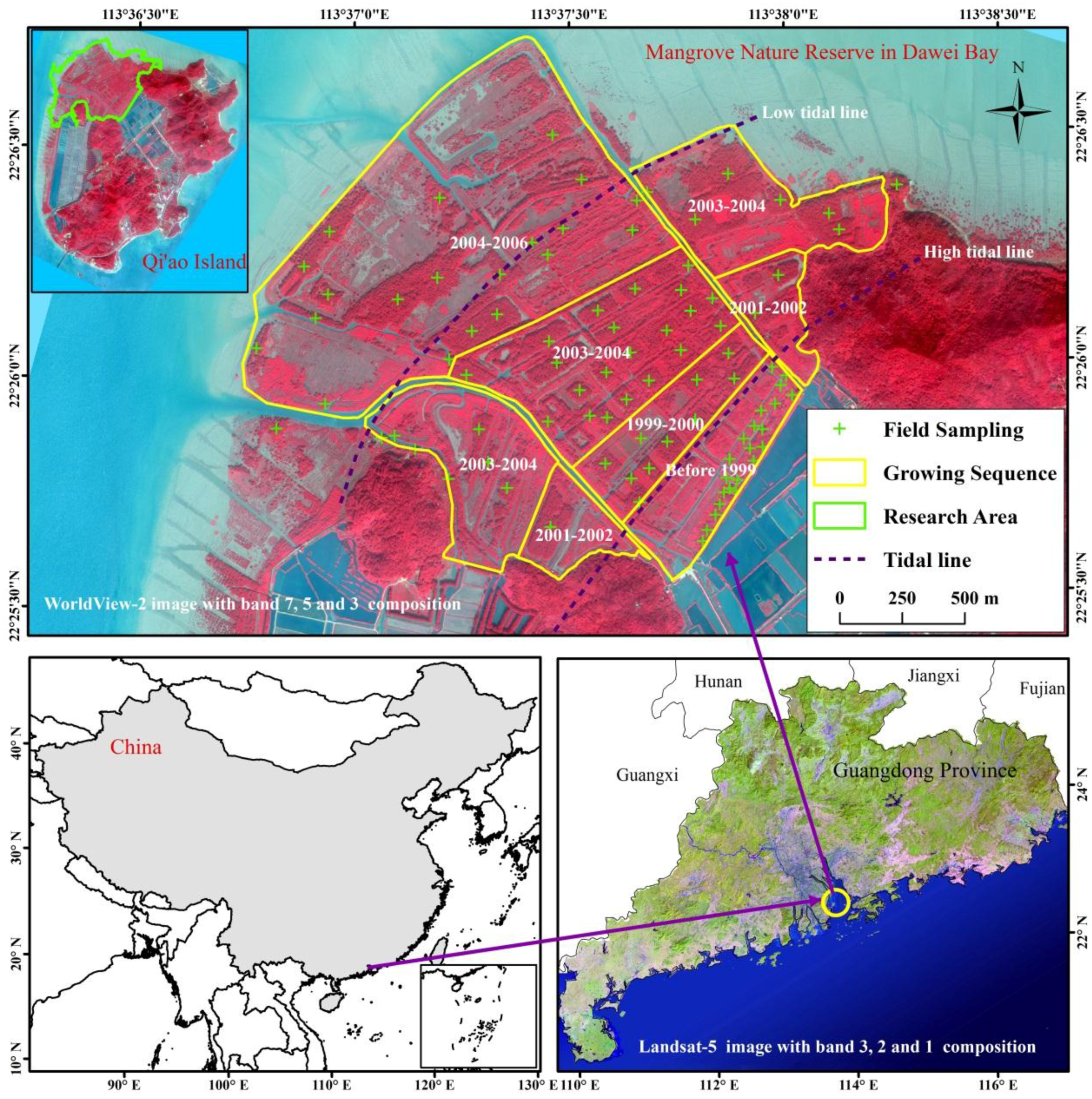
2.1. Study Area

Qi’ao Island (22°23′N–22°27′N, 113°36′E–113°39′E) is located in Lingding Bay of the Pearl River Estuary, Guangdong Province, China, near eastern Zhuhai [39]. As a typical tropical–subtropical wetland ecological system in the Pearl River Estuary, Qi’ao Island is the largest conservation area for artificially restored mangroves in China, covering an area of approximately 700 ha [40,41]. Forests within this dynamic landscape are characterized by uneven-aged trees and high spatial variability.

We investigated remote AGB estimation of uneven-aged mangrove forests based on prevalent mature and native Kandelia candel (K. candel) and artificially restored Sonneratia apetala (S. apetala). They are mainly tree species homogeneously covered by only one of the species in study area. Vegetation grades from widespread mature stands of native K. candel located outside the enclosing levee in the high tidal zones, to artificially-restored S. apetala stands and smaller trees, shrubs, and herbaceous vegetation located progressively closer to the low tidal zones [41,42]. S. apetala and K. candel are the primary mangrove species on Qi’ao Island [43]. K. candel is distributed primarily in a small area along a northeast to southwest direction, as well as in tall and dense stands in the high tidal zone, and the stand has an age of approximately 45 years and tree height of 5.5–7.5 m. S. apetala was first planted in 1999 and is mainly distributed in the middle and low tidal zones. The fast-growing trees have increased in height about 1.5 m each year [44]. Tree height ranges from 2 m to 18 m. S. apetala generally has an afforestation specification of 1.0–2.0 m × 1.5m. The afforestation process has shown a trend of moving from medium to the low tidal zones over time. We found a gradient distribution for tree age and AGB from the high tidal zones to low tidal zones (Figure 1).

Beyond that, a large area of S. alterniflora is distributed outside the tidal flat area, which is the reconstructed demonstration area for S. alterniflora management. Small amounts of A. ilicifolius, Acrostichum aureum (A. aureum), A. corniculatum, Phragmites australis (P. australis) and mangrove nurseries also exist. The regional position is shown in Figure 1.

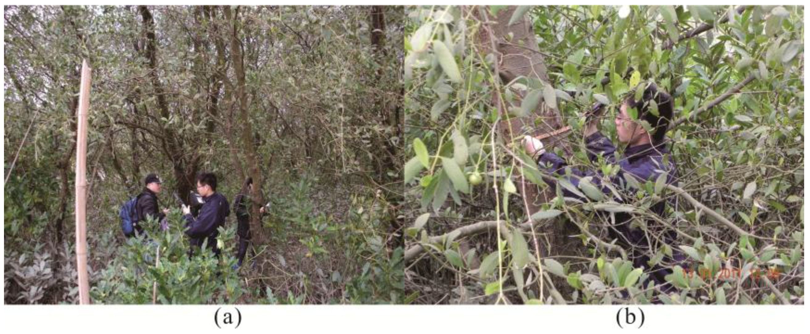
2.2. Field Investigation and Estimation of Mangrove Vegetation Biomass

Field investigation for this research was conducted in two periods: 23 December to 27 December 2010 and 10 January to 15 January 2011. Biomass samples were obtained through random sampling technique along almost all of accessible tidal creeks of Dawei Bay, Qi’ao Island, and covered most of the study area ensuring all of the biomass variation of tree stage represented. Field data were collected on 91 rectangular plots (Figure 1), including 68 plots of artificially restored S. apetala and 23 plots of native, mature K. candel with a 10 m × 10 m quadrat in each sample plot. In order to generate regressions for the allometric equations, we measured the height using a handheld laser range finder (referred to as laser heights with precision of 1m; Trueyard SP-1500H, Trueyard Optical Instruments co.) and diameter at breast height (DBH) (1.3 m) of every tree and recorded the number of trees (Figure 2a,b) within each plot. This study only considered trees with DBH ≥ 5 cm. GPS (Gamin GPS map 60CS) was used to record the longitude and latitude of the quadrat center.

Figure 1. Location, planting sequence, and field sampling sites in the Qi’ao Island mangroves overlaid on a Worldview-2 images (band 7, 5, 3 false color combination) dated 11 November 2010. (Coordinate system: Universal Transverse Mercator Zone 49N, WGS84)

Figure 1. Location, planting sequence, and field sampling sites in the Qi’ao Island mangroves overlaid on a Worldview-2 images (band 7, 5, 3 false color combination) dated 11 November 2010. (Coordinate system: Universal Transverse Mercator Zone 49N, WGS84)

Since mangrove forests are protected in the Nature Reserve, allometric growth equations for S. apetala and native K. candel cannot be established by destructive measurements. Qijie Zan et al. published allometric growth equations for the exotic species (S. apetala and Sonneratia caseolaris (S. caseolaris)) and K. candel from the Pearl River in Shenzhen [45]. Since their study site is only 40 km away from our study site, and both sites are at similar latitudes with comparable environmental settings that retain the same mangrove species, it is reasonable to assume that the equations developed in their study are applicable to this study without any significant error and uncertainty. Therefore, individual tree DBH and height measurements were converted to AGB estimates via allometric equations and then summed over the plot. The range of AGB was calculated from their regression equations (Table 1).

Figure 2. Field investigation of mangrove areas: (a) quadrate investigation for mangrove species and (b) DBH measurement for S. apetala.

Figure 2. Field investigation of mangrove areas: (a) quadrate investigation for mangrove species and (b) DBH measurement for S. apetala.

Table 1. Allometric equations for mangrove forests based on DBH and height referenced Qijie Zan et al. [45].

Species	Tissues	Allometric Equations	Correlation
S. apetala	Foliage	lgWlf = −0.756 + 0.4355 lg (DBH2 × Height)	0.94
	Branch	lgWbr = 0.1590 + 0.3879 lg (DBH2 × Height)	0.95
	Trunk	lgWst = 0.3067 + 0.3302 lg (DBH2 × Height)	0.95
	Bark	lgWba = −0.3790 + 0.3559 lg (DBH2 × Height)	0.91
	Flowers and fruit	lgWfr = −2.3456 + 0.3791 lg (DBH2 × Height)	0.97
K. candel	Foliage	lgWlf = −1.1704 + 0.4855 lg (DBH2 × Height)	0.87
	Branch	lgWbr = −0.9067 + 0.5762 lg (DBH2 × Height)	0.95
	Trunk and bark	lgWst+ba = −0.3112 + 0.2542 lg (DBH2 × Height)	0.88
	Flowers and fruit	lgWfr = −3.1582 + 1.061 lg (DBH2 × Height)	0.85

Table 1. Allometric equations for mangrove forests based on DBH and height referenced Qijie Zan et al. [45].

Species	Tissues	Allometric Equations	Correlation
S. apetala	Foliage	lgWlf = −0.756 + 0.4355 lg (DBH2 × Height)	0.94
	Branch	lgWbr = 0.1590 + 0.3879 lg (DBH2 × Height)	0.95
	Trunk	lgWst = 0.3067 + 0.3302 lg (DBH2 × Height)	0.95
	Bark	lgWba = −0.3790 + 0.3559 lg (DBH2 × Height)	0.91
	Flowers and fruit	lgWfr = −2.3456 + 0.3791 lg (DBH2 × Height)	0.97
K. candel	Foliage	lgWlf = −1.1704 + 0.4855 lg (DBH2 × Height)	0.87
	Branch	lgWbr = −0.9067 + 0.5762 lg (DBH2 × Height)	0.95
	Trunk and bark	lgWst+ba = −0.3112 + 0.2542 lg (DBH2 × Height)	0.88
	Flowers and fruit	lgWfr = −3.1582 + 1.061 lg (DBH2 × Height)	0.85

2.3. Remotely Sensed Data and Processing

WorldView-2 provides satellite images with eight multispectral bands (Table 2), and has advantages over other high spatial-resolution satellite images (i.e., IKONOS, QuickBird, and SPOT5) in terms of acquisition, revisit cycles, geometric accuracy, and multispectral bands [46,47]. WorldView-2 is the only commercial, high spatial resolution satellite imagery that provides a coastal zone band, a yellow band, a red edge band, and a near infrared 2 band. In particular, the red edge band is directly related to chlorophyll level, which reflects the growth condition of vegetation. To a certain extent, the red edge band is more sensitive to biomass at high densities than other bands such as near infrared band canopies (i.e., mangrove forests) [48,49]. The high spatial resolution of WorldView-2 images makes it possible to distinguish different mangrove species, which in turn helps improve the accuracy of mangrove biomass estimation. The WorldView-2 satellite image data with 2 m multispectral resolution was acquired on 11 November 2010.

Table 2. Satellite spectrum and spatial resolution parameters of WorldView-2.

Wavebands		Spectral Band Edges	Spatial Resolution
B1	coastal band	400 nm to 450 nm	2 m
B2	blue band	450 nm to 510 nm	2 m
B3	green band	510 nm to 580 nm	2 m
B4	yellow band	585 nm to 625 nm	2 m
B5	red band	630 nm to 690 nm	2 m
B6	red-edge band	705 nm to 745 nm	2 m
B7	near-infrared-1 band	770 nm to 895 nm	2 m
B8	near-infrared-2 band	860 nm to 1040 nm	2 m

Table 2. Satellite spectrum and spatial resolution parameters of WorldView-2.

Wavebands		Spectral Band Edges	Spatial Resolution
B1	coastal band	400 nm to 450 nm	2 m
B2	blue band	450 nm to 510 nm	2 m
B3	green band	510 nm to 580 nm	2 m
B4	yellow band	585 nm to 625 nm	2 m
B5	red band	630 nm to 690 nm	2 m
B6	red-edge band	705 nm to 745 nm	2 m
B7	near-infrared-1 band	770 nm to 895 nm	2 m
B8	near-infrared-2 band	860 nm to 1040 nm	2 m

In this process, the Worldview-2 image was geo-rectified to a 1:10,000 topographic map using ground control points based on the image-to-map method, followed by radiometric calibration using the sensor calibrating model of calibration utilities. The image was also corrected using the fast line-of-sight atmospheric analysis of the spectral hypercubes (FLAASH) model with the ENVI module (ENVI 5.1) [50]. The major input parameters of FLASSH were mid-latitude summer model (MLS), MODTRAN spectral resolution of 15 cm⁻¹, urban aerosol model, atmospheric water vapor of 2.9 g/cm², and DISORT streams 8 for multiscatter model of Scaled DISORT. The longitude and latitude values recorded in the field survey were considered the central points to calculate the mean vegetation index value in a periphery 5 × 5 grid (10 m × 10 m), with the central point included for the preprocessed image. The calculated value was regarded as the vegetation index of the quadrat.

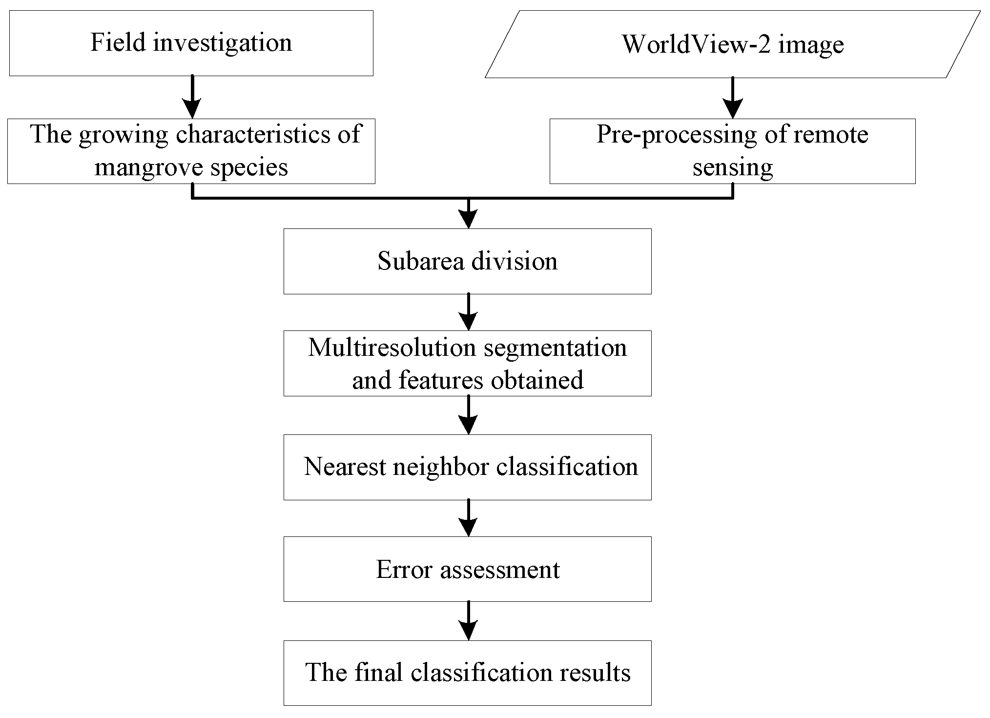
2.4. Mangrove Classification Based on WorldView-2 Images

In this study, we focused on the AGB estimation at the species level using WorldView-2 images. The spatial distribution of the individual species was obtained by using object-oriented classification method and the nearest neighbor classifier, with separate training and validation samples. Since the target objects, S. apetala and K. candel, are mainly tree species homogeneously covered in study area, they can be separated from other objects using hard classification with nearest neighbor classifier. Figure 3 shows the flow chart of mangrove species classification.

Figure 3. Flow chart of mangrove species classification based on WorldView-2 images.

Figure 3. Flow chart of mangrove species classification based on WorldView-2 images.

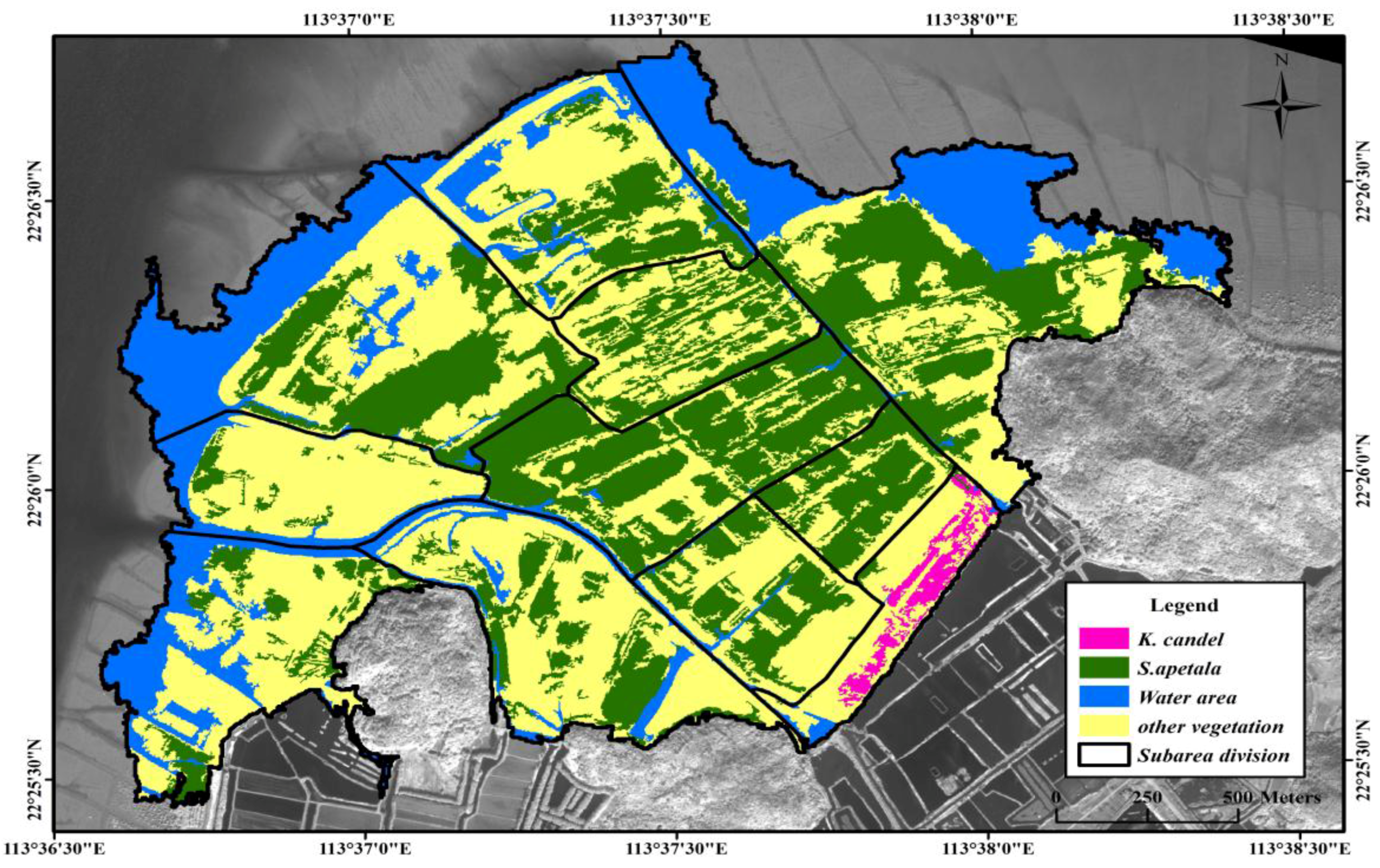
2.4.1. The Characteristics and Spatial Distribution of Mangrove Species

The growing characteristics and spatial distributions of different vegetation types on Qi’ao Island are presented in Table 3. S. apetala and K. candel are the dominant tree species in study area, and other types of vegetation mainly include shrubs and herbaceous vegetation. To improve classification accuracy of mangrove species, the study area was further divided into 11 subareas based on spatial features and the age of the different mangrove species (Figure 4).

Table 3. The characteristics of the different land cover types in Qi’ao Island.

Land Cover Types		Characteristics and Spatial Distribution Features
Target objects	S. apetala	The tree species are tallest in height, distributed in medium to low tidal zones and occupied the largest area on Qi’ao Island.
	K. candel	The tree species are mainly located outside the enclosing levee in the high tidal zones.
Other vegetation		Other vegetation types, including shrubs (A. corniculatum and A. ilicifolius) and herbaceous (S. alterniflora and P. australis) vegetation, are mainly distributed in medium and low tidal zones.

Table 3. The characteristics of the different land cover types in Qi’ao Island.

Land Cover Types		Characteristics and Spatial Distribution Features
Target objects	S. apetala	The tree species are tallest in height, distributed in medium to low tidal zones and occupied the largest area on Qi’ao Island.
	K. candel	The tree species are mainly located outside the enclosing levee in the high tidal zones.
Other vegetation		Other vegetation types, including shrubs (A. corniculatum and A. ilicifolius) and herbaceous (S. alterniflora and P. australis) vegetation, are mainly distributed in medium and low tidal zones.

2.4.2. Image Segmentation

The mangrove species classification is based on an object-oriented method in eCognition 9.0 software, which operates on image objects that have been extracted through image segmentation, rather than on individual pixels [51]. The segmentation technique in eCognition 9.0 is a bottom-up region merging technique where smaller image objects are merged into larger ones with the scale parameter controlling the growth in heterogeneity between adjacent image objects. The merging is stopped when image object growth exceeds the threshold defined by the scale parameter—the maximum allowable heterogeneity of image object [52]. Adjusting the scale parameter influences the average object size. A small value of scale parameter results in the decrease of the average size of image objects. The color parameter, ranging from 0 to 1, determines the weight of spectral (color) heterogeneity against shape heterogeneity in the total image object heterogeneity. Previous studies suggest that more meaningful objects are extracted with a higher weight for the color criterion [52,53]. The shape heterogeneity is further defined as a weighted sum of smoothness (the ratio of the border length and the shortest possible border length of the bounding box of an image object) and compactness (the ratio of the border length and the square root of the number of object pixels). The compactness parameter (0–1) gives the weight of the compactness versus the smoothness in the shape heterogeneity [54].

Ideal object-oriented segments should cover singular entities outlining objects of homogeneous appearance without over or under segmentation [55]. In this study, the segmentation parameters (scale parameter, shape index, compactness index, color index, and smoothness index) were continuously adjusted through repeated experiments and comparison of the segmentation results, the parameter values that produced the best visual effect with singular entities outlining objects of homogeneous appearance were selected [55].

2.4.3. The Classification for Mangrove Species

The nearest neighbor algorithm is a non-parametric method used for the classification of mangrove species [56]. The input features of the training samples consist of a multi-dimensional feature space, each sample with a class label. A test point is classified by assigning the label which is most frequent among the training samples with nearest distance to that test point [57]. A commonly used distance metric for continuous variables is Euclidean distance. The following 14 image attributes were input variables to train and construct the classifier:

(1)

8 spectral attributes: mean values of 8 bands of WorldView-2 for each image object;

(2)

5 shape attributes: area, density, length/width, shape index, and width of each image object;

(3)

1 vegetation attribute: NDVI for each image object.

Every subarea was classified separately using above 14 attributes and the nearest neighbor classifier based on the same optimal segmentation parameters. Half of the collected samples were used for training and the other half for validation. The evaluation of performance was carried out for the species classification by confusion matrix.

2.5. Calculation of Vegetation Indices

Vegetation indices are computed from combinations of different bands. Previous studies have shown that remotely sensed data is closely related to the biophysical parameters of vegetation [58]. External influences, such as sun angle, cloud, terrain, shadow, satellite observation angle, leaf angle, soil background, and plant canopy, etc., can be effectively minimized through a combination of different bands [59,60]. In this study, B5 (red band), B7 (near-infrared-1 band) and B8 (near-infrared-2 band) of the Worldview-2 images were used to calculate six vegetation indices, including the normalized difference vegetation index (NDVI), the simple ratio index (SRI), and the difference vegetation index (DVI) [61]. The indices are computed as:

$$NDV{I}_{75}=\frac{{\text{ρ}}_{B7}-{\text{ρ}}_{B5}}{{\text{ρ}}_{B7}+{\text{ρ}}_{B5}}$$

(1)

$$NDV{I}_{85}=\frac{{\text{ρ}}_{B8}-{\text{ρ}}_{B5}}{{\text{ρ}}_{B8}+{\text{ρ}}_{B5}}$$

(2)

$$SR{I}_{75}=\frac{{\text{ρ}}_{B7}}{{\text{ρ}}_{B5}}$$

(3)

$$SR{I}_{85}=\frac{{\text{ρ}}_{B8}}{{\text{ρ}}_{B5}}$$

(4)

$$DV{I}_{75}={\text{ρ}}_{B7}-{\text{ρ}}_{B5}$$

(5)

$$DV{I}_{85}={\text{ρ}}_{B8}-{\text{ρ}}_{B5}$$

(6)

Apart from the near infrared band, the red edge band is useful in studying precision agriculture, plant phenology, and vegetation biomass. Three vegetation indices based on the red edge band (red-edge NDVI (RE-NDVI), red-edge SRI (RE-SRI), and modified red-edge SRI (mRE-SRI)) were selected for the inversion study. The computational formulas are as follows:

$$RE\text{-}NDV{I}_{65}=\frac{{\text{ρ}}_{B6}-{\text{ρ}}_{B5}}{{\text{ρ}}_{B6}+{\text{ρ}}_{B5}}$$

(7)

$$RE\text{-}SR{I}_{65}=\frac{{\text{ρ}}_{B6}}{{\text{ρ}}_{B5}}$$

(8)

$$mRE\text{-}SR{I}_{651}=\frac{{\text{ρ}}_{B6}-{\text{ρ}}_{B1}}{{\text{ρ}}_{B5}+{\text{ρ}}_{B1}}$$

(9)

In this study, the predictors, including the eight bands derived from WorldView-2 and above nine vegetation indices, and the mangrove AGB samples were used as input parameters to build, test and predict mangrove forest AGB estimation with ANN model.

2.6. Biomass Modeling Accuracy Assessment

A BP ANN was used to estimate AGB of uneven-aged mangrove forests. An ANN is a mathematical model inspired by biological neural networks and has strong abilities of linear and nonlinear fitting. The ANN algorithm adopted in this study is a nonlinear layered feed-forward model with standard back propagation [38,62]. This learning algorithm uses an iterative gradient descent training procedure. The neurons in each layer only affect the neurons in next layer. The initial ANN weights are assigned randomly, and adjusted through a back propagation mechanism. The weight adjusting process is repeated until the model output reaches an acceptable level of accuracy.

In this study, an independent validation dataset was not available for the models accuracy estimation due to the limited number of samples. An iterated 5-fold cross-validation (CV) process was performed to assess the accuracy, stability, reliability and generalization ability of the model [63]. Each iteration uses 80% of samples for training, and 20% of samples for validation. We divided the samples points of each species into 3 parts in terms of AGB values for stratified random sampling, which ensures that each subsample contains the whole range of AGB values. Five iterations were carried out, and the RMSEs of the individual iterations were averaged to yield the overall accuracy.

The ANN algorithm was used to develop AGB model of uneven-aged mangrove forests using the 64-bit vision of Matlab 7.0 for Windows. The model building, tuning and accuracy evaluation were performed by the “Neural Network Toolbox” using the iterated cross-validation (CV) process and stratified random sampling. The main tuning parameters for network (including the number of hidden layer neurons, network iterations, transmission functions of the hidden and output layers) were continuously adjusted by comparing the root mean square error (RMSE) between the measured and estimated biomass to determine the optimal network model [64]. The values of learning rate and training accuracy were 0.01 and 0.001, respectively. Other parameters used the default values in “Neural Network Toolbox” [65]. All the variables, including above vegetation indices (NDVI₇₅, SRI₇₅, DVI₇₅ NDVI₈₅, SRI₈₅, DVI₈₅, RE-NDVI₆₅, RE-SRI₆₅, and mRE-SRI₆₅₁) and image-derived bands, species types and measured biomass were normalized. After normalization, they were used as the input and output variables of the BP ANN model, respectively.

To quantify the effect of mangrove species information on AGB estimation accuracy, we conducted three different experiments to build BP ANN models of mangrove species. In experiment 1 (Expt.1 for short), we did not distinguish the individual species and built a single BP ANN model for the mixture of above species. This model is named the Mixed Species Model. In experiment 2 (Expt.2), a dummy variable indicating S. apetala or K. candel as an extra variable is added to the Mixed Species Model. The model is named the Dummy Species Model. In experiment 3 (Expt.3), we built a separate BP ANN model for each of the two individual species, respectively. The models are named the Individual Species Models.

After building the BP ANN models of mangrove forests biomass, indicators of RMSE, relative RMSE (RMSE_r) were utilized to estimate models accuracy by analyzing the measured and predicted values. Their computational formulas are as follows:

$$RMSE=\sqrt{\frac{{{\displaystyle \sum (y_i-{\widehat{y}}_i)}}^2}{n}}$$

(10)

$$RMS{E}_r=\frac{RMSE}{\overline{y}}$$

(11)

where $y_i$ (i=1,2,…,n) and $\widehat{y_i}$ represent the actual and predicted value of AGB at plot i based on validation data, respectively where as $\overline{y}$ represents actual average of AGB. n is the number of validation plots.

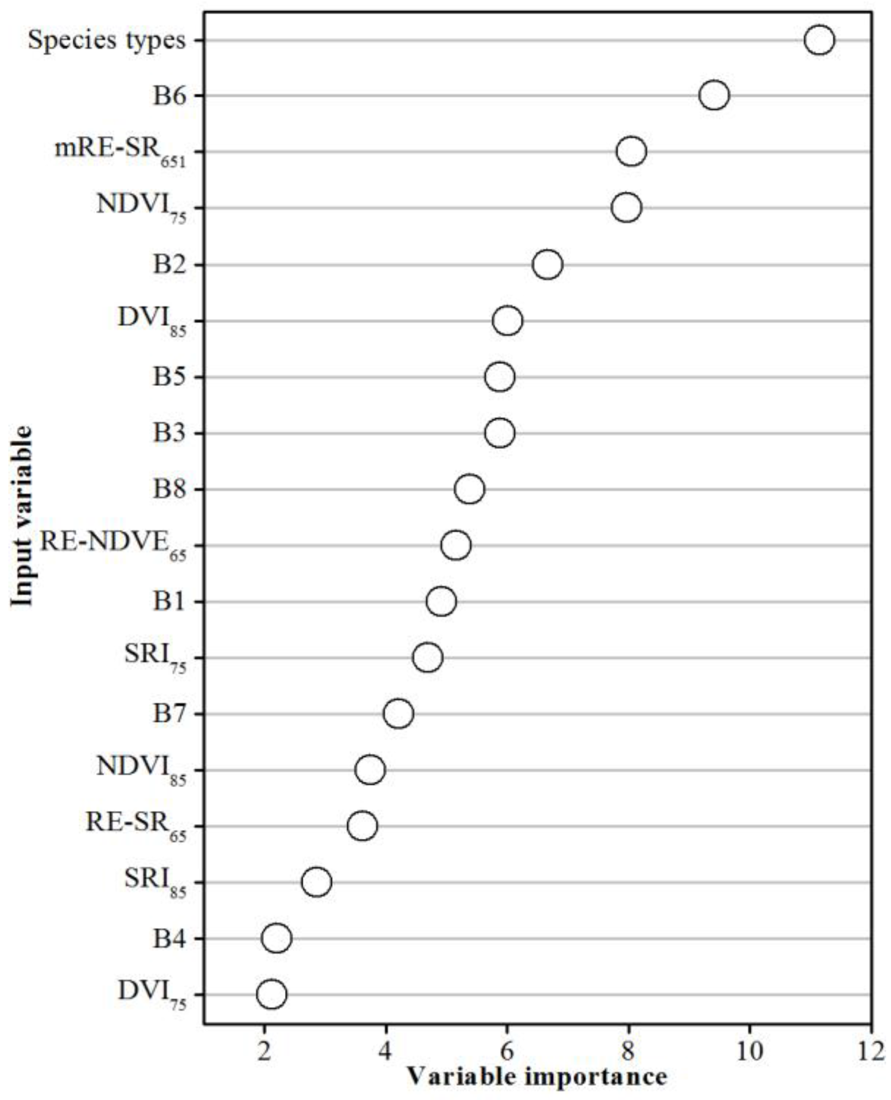
2.7. Importance of the Variables

The contribution of each input variable to mangrove AGB estimation (including the eight bands from Worldview-2 image, above nine vegetation indices and species) was quantified by using the whole sample dataset and “Weights” method applied to the Dummy Species Model [66]. The relative importance of an input variable was determined by partitioning the connection weights of the ANN model, involving partitioning the hidden-output connection weights of each hidden layer’s neuron into components associated with each input neuron [67]. The input-hidden layer connection weight was divided by the sum of the absolute value for all input neurons. The hidden-output layer connection weight was divided by the sum for each hidden neuron of the sum for each input neuron. The relative importance of the given input variable is then obtained by all output weights.

3. Results

3.1. Mangrove Classification at Species Level

On the basis of the multi-resolution segmentation by object-oriented nearest neighbor classification, the optimal spatial scale parameters for the mangrove species classification in this study were selected as follows: scale parameter (30), shape index (0.3), compactness index (0.4), color index (0.7), and smoothness index (0.6). On the basis of field survey data and the prior knowledge, the study area was further divided into 11 subareas (Figure 4), which were classified separately by means of a nearest neighbor classifier. According to the object type of the subarea, four different land cover types were correctly classified, including: K. candel, S. apetala, other vegetation, and water area.

With uncertainty factors influencing the imaging, analysis and classification process, a difference exists between the classification of the remote sensing images and the actual terrain coverage. Therefore, the accuracy of the classification results was evaluated on the basis of the validation dataset obtained from field survey (Table 4). The total classification accuracy was 87.68% and the Kappa coefficient was 0.82. The classification results are shown in Figure 4, and the areas of S. apetala and K. candel were 137.74 ha and 4.24 ha, respectively.

Table 4. Confusion matrix of object-oriented classification for mangrove species.

Classified Data	Reference Data
	K. candel	S. apetala	Other Vegetation	Water Area	Total	User’s Accuracy
K. candel	68	0	8	0	76	89.47%
S. apetala	0	252	30	0	282	89.36%
Other vegetation	12	48	339	13	412	82.28%
Water area	0	0	12	216	228	94.74%
Total	80	300	389	229	998
Producer’s accuracy	85.00%	84.00%	87.15%	94.32%
Overall accuracy: 87.68%；Kappa：0.82

Table 4. Confusion matrix of object-oriented classification for mangrove species.

Classified Data	Reference Data
	K. candel	S. apetala	Other Vegetation	Water Area	Total	User’s Accuracy
K. candel	68	0	8	0	76	89.47%
S. apetala	0	252	30	0	282	89.36%
Other vegetation	12	48	339	13	412	82.28%
Water area	0	0	12	216	228	94.74%
Total	80	300	389	229	998
Producer’s accuracy	85.00%	84.00%	87.15%	94.32%
Overall accuracy: 87.68%；Kappa：0.82

Figure 4. Subarea division and classified map of the mangrove vegetation on Qi’ao Island.

Figure 4. Subarea division and classified map of the mangrove vegetation on Qi’ao Island.

3.2. Estimation of Mangrove Vegetation Biomass

Biomass was calculated through allometric equations (Table 5). The first three parameters in Table 5 are derived from our field observations. The native K. candel has a density of 5257 trees per ha. Biomass ranges from 170.96 t/ha to 448.19 t/ha, with an average of 273 t/ha. S. Apetala has a growing density 1860 trees per ha. Biomass ranges from 37.44 t/ha to 258.17 t/ha, with an average of 125.49 t/ha. The biomass of the former is significantly greater than the latter because K. candel is a native species, approximately 40 years of age, and a much higher growing density than S. apetala.

Table 5. Biomass of K. candel and S. apetala in field sampling.

Species	Average Height(m)	Average DBH (cm)	Number of Trees per ha	Range of Biomass (t/ha)	The Mean of AGB (t/ha)	Standard Deviations (t/ha)
K. candel	6.62	8.32	5257	170.96~448.19	272.97	67.27
S. apetala	11.41	13.23	1860	37.44~258.17	125.49	55.23

Table 5. Biomass of K. candel and S. apetala in field sampling.

Species	Average Height(m)	Average DBH (cm)	Number of Trees per ha	Range of Biomass (t/ha)	The Mean of AGB (t/ha)	Standard Deviations (t/ha)
K. candel	6.62	8.32	5257	170.96~448.19	272.97	67.27
S. apetala	11.41	13.23	1860	37.44~258.17	125.49	55.23

3.3. The Relationship between the Biomass and the Selected Variables

Application of the “Weights” method to the built Dummy Species Model revealed the importance values of all variables including the eight bands from Worldview-2 image and the above nine vegetation indices and species (Figure 5). The results indicate that species type is the most important variable. Incorporation of species type is the key for improving the AGB estimation accuracy. The next two most important variables are the B6 and mRE-SR₆₅₁, indicating B6 and the derived vegetation indices to be more valuable than other bands and their associated vegetation indices in AGB estimation.

Figure 5. Ranked variable importance based on “Weights” method based on the built Dummy Species Model.

Figure 5. Ranked variable importance based on “Weights” method based on the built Dummy Species Model.

3.4. Model Results and Accuracy Test

The BP ANN models were developed using AGB as the output variables and selected predictors derived from Worldview-2 images and species types as input variables. The accuracies of the BP ANN models were tested though RMSE based on above three different experiments (Table 6). The estimation accuracies of the BP ANN models in Expt.2 and Expt.3 were significantly better than the Mixed Species Model in Expt.1. The estimation accuracy at the mixed species level produced the highest RMSE (72.26 t/ha, 43.14% of the average AGB). Expt. 2, with the inclusion of a dummy species variable, performed much better than the Mixed Species Model, with a 19.17% decrease in RMSE. Overall, the Individual Species Model in Expt. 3 performed the best, with S. apetala having the lowest RMSE (24.32 t/ha, 18.97% of the average AGB) and K. candel a low RMSE (52.38 t/ha, 19.52% of the average AGB).

Table 6. The RMSE of biomass estimation among three different experiments.

BP ANN Model		RMSEs (t/ha)					Average RMSE (t/ha)	Average RMSEr (%)
Expt.1	Mixed species	74.41	71.75	82.38	68.80	63.97	72.26	43.14%
Expt.2	Dummy species	40.69	38.23	45.92	33.44	42.45	40.15	23.97%
Expt.3	K. candel	52.12	48.37	49.48	42.23	69.70	52.38	19.52%
	S. apetala	31.54	26.92	22.46	18.27	22.45	24.32	18.97%

Table 6. The RMSE of biomass estimation among three different experiments.

BP ANN Model		RMSEs (t/ha)					Average RMSE (t/ha)	Average RMSEr (%)
Expt.1	Mixed species	74.41	71.75	82.38	68.80	63.97	72.26	43.14%
Expt.2	Dummy species	40.69	38.23	45.92	33.44	42.45	40.15	23.97%
Expt.3	K. candel	52.12	48.37	49.48	42.23	69.70	52.38	19.52%
	S. apetala	31.54	26.92	22.46	18.27	22.45	24.32	18.97%

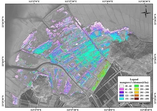
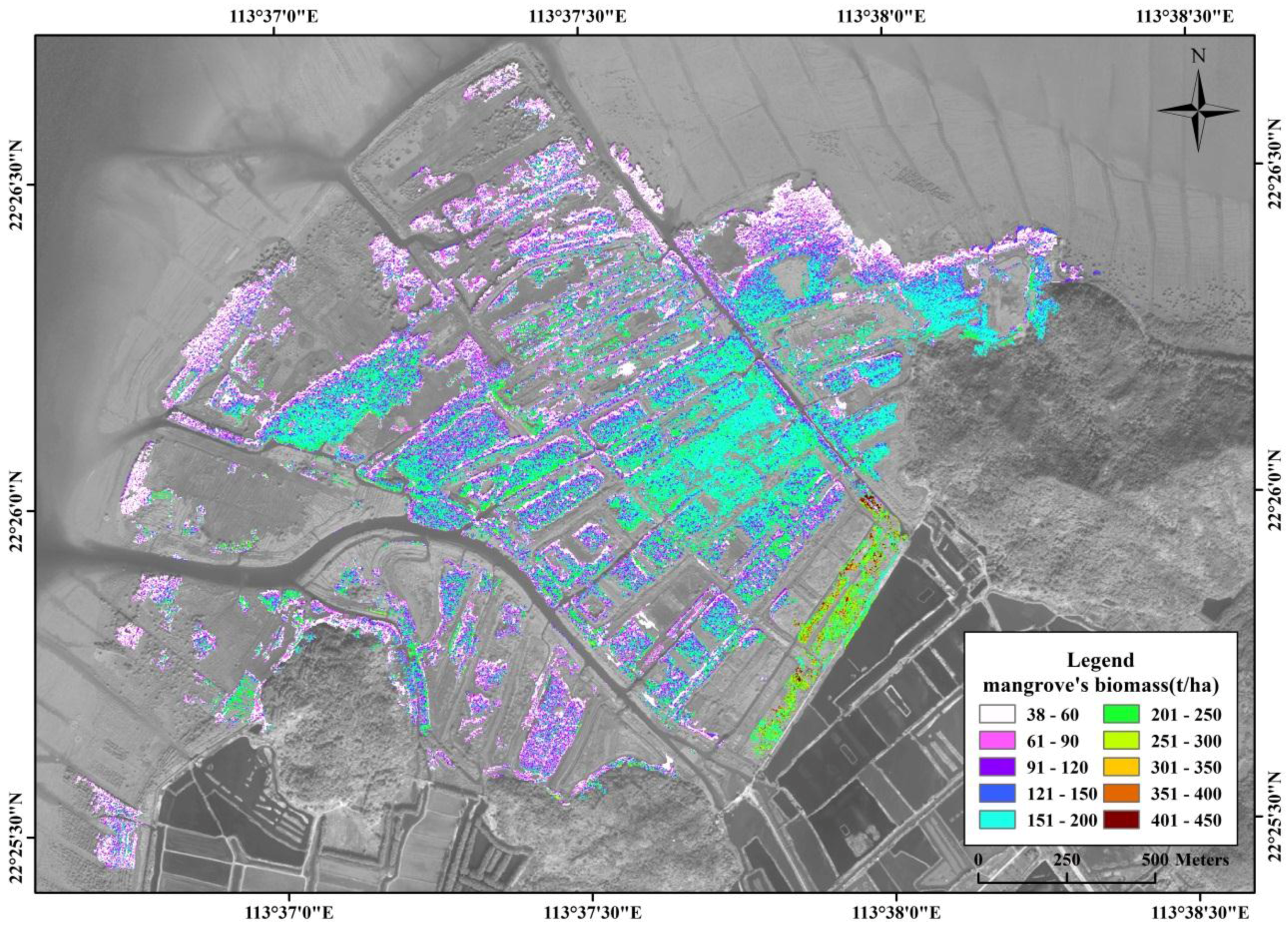
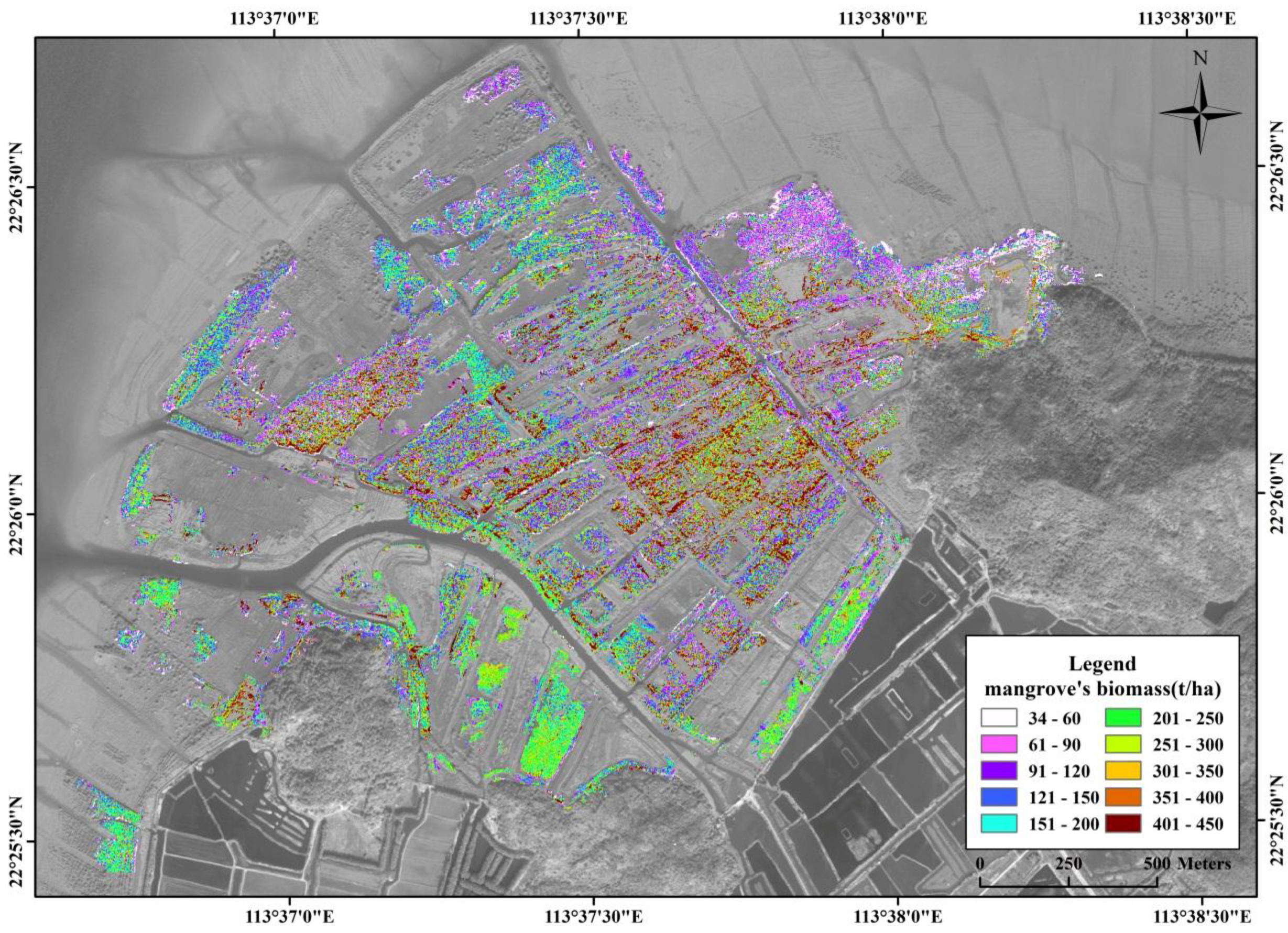
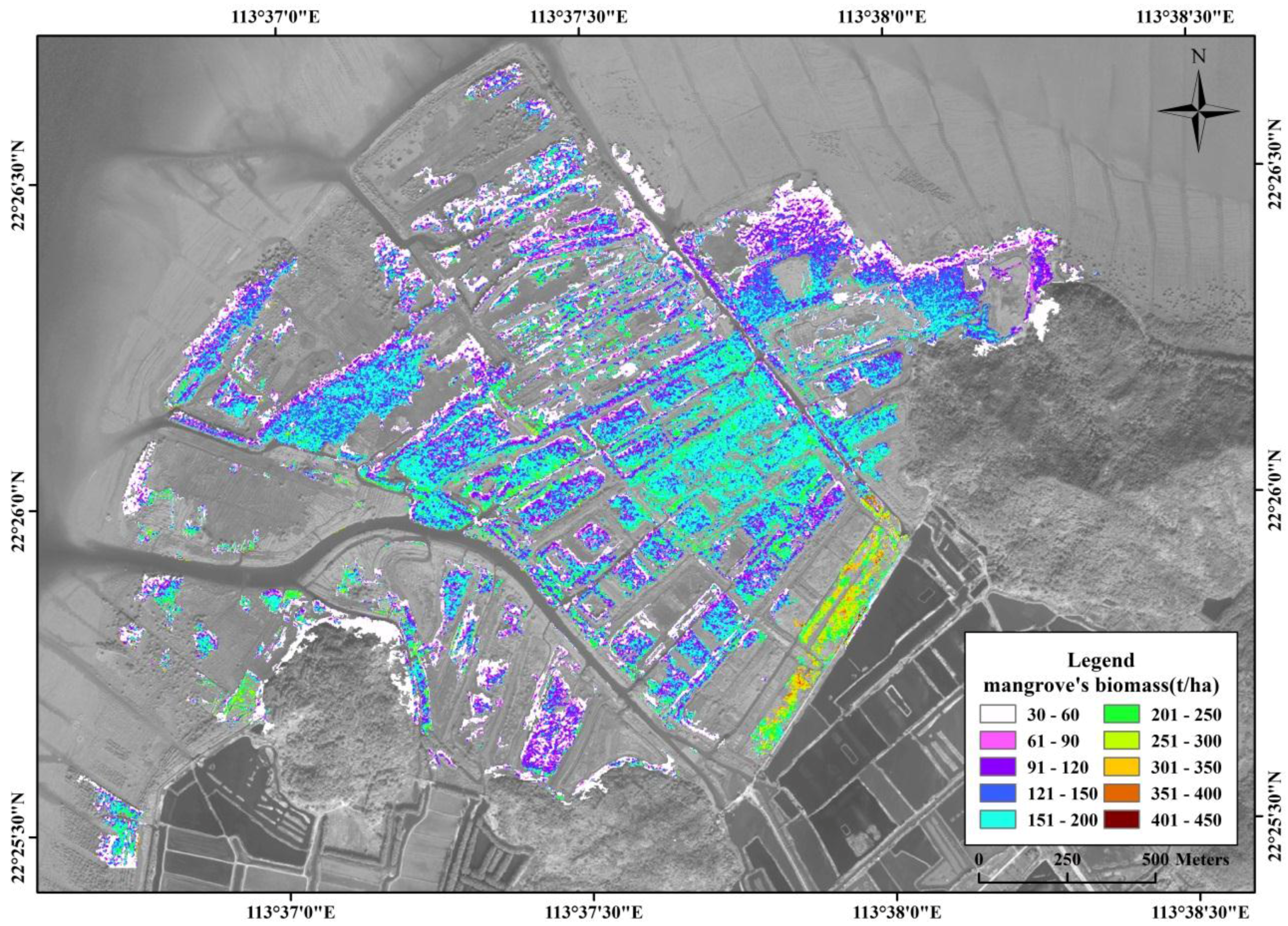
3.5. Spatial Distribution of Mangrove Vegetation Biomass

Spatial distributions of mangrove vegetation biomass in three different experiments are presented in Figure 6, Figure 7 and Figure 8, respectively. In Expt.1 for the mixed species level (Figure 6), AGB of K. candel was underestimated, ranging from 36.23 to 447.26 t/ha, with an average of 212.69 t/ha; whereas that of S. apetala was overestimated, ranging from 33.55 to 446.64 t/ha, with an average of 204.39 t/ha. Comparison with the actual measured values (Table 5) revealed that the biomass predictions obtained by the ANN were not consistent in terms of mean value and distribution range. The highest AGB was S. apetala and mainly distributed in the middle tidal zones. The predicted AGB of K. candel was less than S. apetala distribution at the middle tidal zones.

In Expt.2, for the incorporation the species types as a dummy variable (Figure 7), the accuracy of AGB prediction was much improved over that of Expt. 1. The estimated K. candel AGB ranged from 120.23 to 442.14 t/ha, with an average of 258.84 t/ha; whereas that of S. apetala was between 30.42 and 321.99 t/ha, with an average of 131.32 t/ha. Comparison with the actual measured values (Table 5) revealed that the biomass mean value obtained by the ANN was consistent with the actual mean, but the biomass range was a little different from the actual distribution range. The spatial distribution pattern was also in accordance with the field investigation.

In Expt.3, for the individual species level (Figure 8), AGB prediction of K. candel was mainly between 174.13 and 448.47 t/ha, with an average of 263.21 t/ha; whereas that of S. apetala was between 37.65 and 257.86 t/ha, with an average of 128.15 t/ha. The above results revealed that the predictions of spatial distribution of biomass are consistent with the observation in terms of the actual mean and distribution range (Table 5). The predicted K. candel was mainly distributed in the high tidal zones, and the predicted S. apetala mainly in the middle tidal zones, especially in the central portion of the study area. The experimental results matched the field study very well.

Figure 6. Spatial distribution of mangrove vegetation biomass at the mixed species level based on the artificial neural network (ANN) model in Expt.1.

Figure 6. Spatial distribution of mangrove vegetation biomass at the mixed species level based on the artificial neural network (ANN) model in Expt.1.

Figure 7. Spatial distribution of mangrove vegetation biomass at the incorporation of species as a dummy variable based on the ANN model in Expt.2.

Figure 7. Spatial distribution of mangrove vegetation biomass at the incorporation of species as a dummy variable based on the ANN model in Expt.2.

Figure 8. Spatial distribution of mangrove vegetation biomass at the individual species level based on the ANN model in Expt.3.

Figure 8. Spatial distribution of mangrove vegetation biomass at the individual species level based on the ANN model in Expt.3.

4. Discussion

4.1. Biomass Estimation Accuracy Involving Species Types

The results above revealed that species type was the most important variable among all input parameters for mangrove AGB estimation in this study. In Expt.3, species-specific BP ANN models had the highest estimation accuracy and were significantly better than the model at the mixed species level in Expt.1.

While the mean of RMSE of Expt. 2 is only slightly higher than that of Expt. 3, the range of the predicted AGB and the spatial distribution is not as accurate as those of Expt. 3. It should be pointed out that the number of samples needed in Expt. 2 is much less than that of Expt. 3. Therefore, when field samples are hard to obtain, the Dummy Species Model of Expt. 2 may be an acceptable alternative to the Individual Species Model in Expt. 3.

Given that optical imagery cannot obtain tree height as a crucial parameter in biomass estimation, detailed and accurate estimation of mangrove forest AGB still presents a challenge when parameters derived from optical imagery are applied to biomass estimation. Studies of plant allometry indicated that biomass is determined not only by canopy parameters but also by other factors such as wood density, trunk taper and tree height [68,69,70], which are closely relevant to the floristic characteristics of the species. As a result, the biomass estimation model depends on canopy parameter and species types [71]. In addition, the spectral differences of different mangrove species should be considered in mangrove AGB estimation [24]. Therefore, species types should be input the models in biomass estimation to improve estimation accuracy. Biomass estimation with consideration of species type information can avoid the weakness of the optical imagery and errors caused by spectrum differences among tree species to some extent.

4.2. The Remote Sensing-Derived Input Variables Contribution to the Mangrove Biomass

This study found that the red edge band or the associated vegetation indices B6 and mRE-NDVI₆₅₁) were more important than other bands in estimating AGB (Figure 5). The results were consistent with the conclusion of the previous research [27]. A reason for the advantage of B6 is that a slight change of vegetation properties will lead to a notable shift in the red edge spectral curve [72]. Therefore, the parameters computed from the red edge band are more sensitive to biophysical parameters of vegetation such as canopy biomass compared to the other bands. The red edge and its derived VI can help resolve saturation of tree biomass estimation to some extent in a densely vegetated mangrove area [27]. Such indices may yield more accurate estimations compared to other bands and its derivative indices.

4.3. Spatial Distribution of Mangrove Vegetation Biomass

Historical data, field investigation, and remote sensing image interpretation of Qi’ao Island were utilized to further verify the rationality and accuracy of the models used for estimating mangrove vegetation biomass. The field study showed that K. candel had high individual density and large biomass and small gradient changes in biomass spatial distribution. S. apetala, which was first artificially restored and planted in 1999, generally shows a trend of afforestation from the medium to low tidal zone, based on growing sequence. Thus, its biomass decreases progressively from the medium to the low tidal zone, and trees growing near the medium tidal zone have larger canopies and greater biomass compared with those in other locations. Individuals growing outside the forest edge and near the mudflats were younger and had smaller biomass [73,74].

In the present study, the Worldview-2 images-based ANN models were employed to predict the spatial distribution of the uneven-aged mangrove vegetation biomass. The predicted AGB of K. candel was less than S. apetala distribution at the middle tidal zones for the mixed species in Expt.1 (Figure 6). The results for the mixed species were not consistent with our field investigation.

The biomass estimations of mangrove forest biomass at the individual species level (Expt. 3) or with the incorporation of species type information as a dummy variable (Expt. 2) based on the ANN model were reasonable and in agreement with the field investigation results and known sequences of mangrove afforestation. The biomass of K. candel was largest in specific strips in the study area, whereas the biomass of S. apetala was larger around the middle tidal zone and smaller outside the forest edge and near the mudflats in Expt.2 and 3. Overall, the spatial accuracy of Expt. 3 is better than that of Expt. 2.

5. Conclusions

The main goal of this research was to explore the feasibility and accuracy of a remote sensing model for AGB mapping in uneven-aged and high-density mangrove forests. Our study showed that spatially accurate AGB estimates of mangrove forests can be achieved using the BP ANN model and selected variables derived from WorldView-2 imagery with consideration of species type information.

Our study quantified the contribution of species type information in mangrove biomass estimation. The model incorporating of species type information as a dummy variable improved the accuracy as much as 19.17% in terms of RMSE over the model for the mixed species. The species-specific models reached even higher accuracies. Conventional errors caused by spectrum and height differences among tree species can be avoided by incorporation of species type information using the WorldView-2 images.

In addition, the study confirmed that the red edge band of WorldView-2 and its derived data are more effective in predicting the biomass of high-density mangrove forests than traditional bands. There exists great potential for mapping the spatial distribution and important biophysical elements of mangroves at regional scales with high-resolution multispectral WorldView-2 imagery. Future research will focus on the contributions of red-edge band to the improvement of biomass estimation accuracy. The potential of applying high-resolution Worldview-2 images in inversion of vegetation biomass and other biophysical parameters needs to be fully investigated.

References

1. Myint, S.W.; Giri, C.P.; Wang, L.; Zhu, Z.; Gillete, S.C. Identifying mangrove species and their surrounding land use and land cover classes using object-oriented approach with a lacunarity spatial measure. GISci. Remote Sens. 2008, 45, 188–208. [Google Scholar] [CrossRef]
2. Pendleton, L.H.; Sutton-Grier, A.E.; Gordon, D.R.; Murray, B.C.; Victor, B.E.; Griffis, R.B.; Lechuga, J.A.V.; Giri, C. Considering “Coastal Carbon” in existing U.S. Federal Statutes and Policies. Coast. Manag. 2013, 41, 439–456. [Google Scholar] [CrossRef]
3. Myint, S.W.; Franklin, J.; Buenemann, M.; Kim, W.K.; Giri, C.P. Examining change detection approaches for tropical mangrove monitoring. Photogramm. Engin. Remote Sens. 2014, 80, 983–993. [Google Scholar] [CrossRef]
4. Kankare, V.; Vastaranta, M.; Holopainen, M.; Räty, M.; Yu, X.; Hyyppä, J.; Hyyppä, H.; Alho, P.; Viitala, R. Retrieval of forest aboveground biomass and stem volume with airborne scanning LiDAR. Remote Sens. 2013, 5, 2257–2274. [Google Scholar] [CrossRef] [Green Version]
5. Kosoy, N.; Corbera, E. Payments for ecosystem services as commodity fetishism. Ecol. Econ. 2010, 69, 1228–1236. [Google Scholar] [CrossRef]
6. Kovacs, J.; King, J.; Flores De Santiago, F.; Flores-Verdugo, F. Evaluating the condition of a mangrove forest of the Mexican Pacific based on an estimated leaf area index mapping approach. Environ. Monit. Assess. 2009, 157, 137–149. [Google Scholar] [CrossRef] [PubMed]
7. Lovelock, C. Soil respiration and belowground carbon allocation in mangrove forests. Ecosystems 2008, 11, 342–354. [Google Scholar] [CrossRef]
8. Thapa, R.B.; Watanabe, M.; Motohka, T.; Shimada, M. Potential of high-resolution ALOS-PALSAR mosaic texture for aboveground forest carbon tracking in tropical region. Remote Sens. Environ. 2015, 160, 122–133. [Google Scholar] [CrossRef]
9. Chen, L.Z.; Lin, P.; Wang, W.Q. The Eco-Engineering Problems of Plantable Areas Selection in Mangroves Forestation. Available online: www.paper.edu.cn/download/downPaper/200503-48 (accessed on 14 September 2015). (In Chinese)
10. Peng, Y.; Zhou, Y.; Chen, G. The restoration of mangrove wetland: A review. Acta Ecol. Sin. 2008, 28, 786–797. (In Chinese) [Google Scholar]
11. Jia, M.; Wang, Z.; Zhang, Y.; Ren, C.; Song, K. Landsat-Based estimation of mangrove forest loss and restoration in Guangxi Province, China, influenced by human and natural factors. IEEE J. Sel. Top. Appl. Earth Obs. Remote Sens. 2015, 8, 311–323. [Google Scholar] [CrossRef]
12. Feng, J.; Guo, J.; Huang, Q.; Jiang, J.; Huang, G.; Yang, Z.; Lin, G. Changes in the community structure and diet of benthic macrofauna in invasive Spartina alterniflora Wetlands following restoration with native mangroves. Wetlands 2014, 34, 673–683. [Google Scholar] [CrossRef]
13. Giri, C.; Ochieng, E.; Tieszen, L.L.; Zhu, Z.; Singh, A.; Loveland, T.; Masek, J.; Duke, N. Status and distribution of mangrove forests of the world using earth observation satellite data. Global Ecol. Biogeogr. 2011, 20, 154–159. [Google Scholar] [CrossRef]
14. Heumann, B.W. Satellite remote sensing of mangrove forests: Recent advances and future opportunities. Prog. Phys. Geogr. 2011, 35, 87–108. [Google Scholar] [CrossRef]
15. Hirata, Y.; Tabuchi, R.; Patanaponpaiboon, P.; Poungparn, S.; Yoneda, R.; Fujioka, Y. Estimation of aboveground biomass in mangrove forests using high-resolution satellite data. J. For. Res. 2014, 19, 34–41. [Google Scholar] [CrossRef]
16. Patil, V.; Singh, A.; Naik, N.; Unnikrishnan, S. Estimation of carbon stocks in Avicennia marina stand using allometry, CHN analysis, and GIS methods. Wetlands 2014, 34, 379–391. [Google Scholar] [CrossRef]
17. Ishil, T.; Tateda, Y. Leaf area index and biomass estimation for mangrove plantation in Thailand. In Proceedings of IEEE International Geoscience and Remote Sensing Symposium, Anchorage, AK, USA, 20–24 September 2004; pp. 2323–2326.
18. Proisy, C.; Couteron, P.; Fromard, F. Predicting and mapping mangrove biomass from canopy grain analysis using Fourier-based textural ordination of IKONOS images. Remote Sens. Environ. 2007, 109, 379–392. [Google Scholar] [CrossRef]
19. Ji, M.; Hu, J.; Feng, J. Measuring mangrove biomass via remote sensing subpixel analysis. Remote Sens. Model. Ecosyst Sustain. 2010, 7809. [Google Scholar] [CrossRef]
20. Lucas, R.M.; Mitchell, A.L.; Rosenqvist, A.; Proisy, C.; Melius, A.; Ticehurst, C. The potential of L-band SAR for quantifying mangrove characteristics and change: Case studies from the tropics. Aquat. Conserv. Mar. Freshw. Ecosyst. 2007, 17, 245–264. [Google Scholar] [CrossRef]
21. Li, X.; Yeh, A.G.; Wang, S.; Liu, K.; Liu, X.; Qian, J.; Chen, X. Regression and analytical models for estimating mangrove wetland biomass in South China using Radarsat images. Int. J. Remote Sens. 2007, 28, 5567–5582. [Google Scholar] [CrossRef]
22. Simard, M.; Rivera-Monroy, V.H.; Mancera-Pineda, J.E.; Castañeda-Moya, E.; Twilley, R.R. A systematic method for 3D mapping of mangrove forests based on Shuttle Radar Topography Mission elevation data, ICEsat/GLAS waveforms and field data: Application to Ciénaga Grande de Santa Marta, Colombia. Remote Sens. Environ. 2008, 112, 2131–2144. [Google Scholar] [CrossRef]
23. Chadwick, J. Integrated LiDAR and IKONOS multispectral imagery for mapping mangrove distribution and physical properties. Int. J. Remote Sens. 2011, 32, 6765–6781. [Google Scholar] [CrossRef]
24. Koedsin, W.; Vaiphasa, C. Discrimination of tropical mangroves at the species level with EO-1 hyperion data. Remote Sens. 2013, 5, 3562–3582. [Google Scholar] [CrossRef]
25. Ni-Meister, W.; Lee, S.; Strahler, A.H.; Woodcock, C.E.; Schaaf, C.; Yao, T.; Ranson, K.J.; Sun, G.; Blair, J.B. Assessing general relationships between aboveground biomass and vegetation structure parameters for improved carbon estimate from LiDAR remote sensing. J. Geophys. Res. 2010, 115. [Google Scholar] [CrossRef]
26. Chen, Q.; Vaglio Laurin, G.; Battles, J.J.; Saah, D. Integration of airborne LiDAR and vegetation types derived from aerial photography for mapping aboveground live biomass. Remote Sens. Environ. 2012, 121, 108–117. [Google Scholar] [CrossRef]
27. Mutanga, O.; Adam, E.; Cho, M.A. High density biomass estimation for wetland vegetation using worldview-2 imagery and random forest regression algorithm. Int. J. Appl. Earth Obs. Geoinform. 2012, 18, 399–406. [Google Scholar] [CrossRef]
28. Demuro, M.; Chisholm, L. Assessment of hyperion for characterizing mangrove communities. In Proceedings of the 12th JPL AVIRIS Airborne Earth Science Workshop, Pasadena, CA, USA, 24–28 February 2003.
29. Heenkenda, M.; Joyce, K.; Maier, S.; Bartolo, R. Mangrove species identification: Comparing WorldView-2 with aerial photographs. Remote Sens. 2014, 6, 6064–6088. [Google Scholar] [CrossRef]
30. Eacute, S.; Rapinel, B.; Eacute, B.C.; Ment; Magnanon, S.; Sellin, V.; Hubert-Moy, L. Identification and mapping of natural vegetation on a coastal site using a Worldview-2 satellite image. J. Environ. Manag. 2014, 144, 236–246. [Google Scholar] [Green Version]
31. Mutanga, O.; Skidmore, A.K. Narrow band vegetation indices overcome the saturation problem in biomass estimation. Int. J. Remote Sens. 2004, 25, 3999–4014. [Google Scholar] [CrossRef]
32. Adam, E.M.I.; Mutanga, O. Estimation of high density wetland biomass: combining regression model with vegetation index developed from Worldview-2 imagery. Proc. SPIE 2012, 8531. [Google Scholar] [CrossRef]
33. Eckert, S. Improved forest biomass and carbon estimations using texture measures from worldView-2 satellite data. Remote Sens. 2012, 4, 810–829. [Google Scholar] [CrossRef]
34. Jachowski, N.R.A.; Quak, M.S.Y.; Friess, D.A.; Duangnamon, D.; Webb, E.L.; Ziegler, A.D. Mangrove biomass estimation in Southwest Thailand using machine learning. Appl. Geogr. 2013, 45, 311–321. [Google Scholar] [CrossRef]
35. Breiman, L. Random forests. Mach. Learn. 2001, 45, 5–32. [Google Scholar] [CrossRef]
36. Ciresan, D.; Meier, U.; Schmidhuber, J. Multi-column deep neural networks for image classification. In Proceedings of IEEE Computer Vision and Pattern Recognition (CVPR), Providence, RI, USA, 16–21 June 2012; pp. 3642–3649.
37. Mas, J.F.; Flores, J.J. The application of artificial neural networks to the analysis of remotely sensed data. Int. J. Remote Sens. 2008, 29, 617–663. [Google Scholar] [CrossRef]
38. Wang, L.; Silván-Cárdenas, J.L.; Sousa, W.P. Neural network classification of mangrove species from multiseasonal IKONOS imagery. Photogramm. Engin. Remote Sens. 2008, 74, 921–927. [Google Scholar] [CrossRef]
39. Liu, K.; Li, X.; Wang, S.G.; Liu, W.X. Classification of mangroves by data fusion and neural networks. Remote Sens. Inf. 2006, 3, 32–36. (In Chinese) [Google Scholar]
40. Liu, K.; Li, X.; Shi, X.; Wang, S. Monitoring mangrove forest changes using remote sensing and GIS data With decision-tree learning. Wetlands 2008, 28, 336–346. [Google Scholar] [CrossRef]
41. Wang, S.G.; Li, X.; Zhou, Y.Z.; Liu, K.; Chen, G.Z. The change of mangrove wetland ecosystem and controlling countermeasures in the Qi’ao Island. Wetl. Sci. 2005, 3, 13–20. (In Chinese) [Google Scholar]
42. Liu, K.; Liu, L.; Liu, H.; Li, X.; Wang, S. Exploring the effects of biophysical parameters on the spatial pattern of rare cold damage to mangrove forests. Remote Sens. Environ. 2014, 150, 20–33. [Google Scholar] [CrossRef]
43. Liao, B.W.; Guan, W.; Zhang, J.E.; Tang, G.L.; Lei, Z.S. Studies on Dynamic Development of Mangrove Communities on Qi’ao Island, Zhuhai. J. South China Agric. Univ. 2008, 29, 59–64. (In Chinese) [Google Scholar]
44. Chen, H.; Liao, B.; Liu, B.E.; Peng, C.; Zhang, Y.; Guan, W.; Zhu, Q.A.; Yang, G. Eradicating invasive Spartina alterniflora with alien Sonneratia apetala and its implications for invasion controls. Ecol. Engin. 2014, 73, 367–372. (In Chinese) [Google Scholar] [CrossRef]
45. Zan, Q.J.; Wang, Y.J. Biomass and net productivity of Sonneratia apetala, S.caseolaris mangrove man-made forest. J. Wuhan Bot. Res. 2001, 19, 391–396. (In Chinese) [Google Scholar]
46. Aguilar, M.A.; Saldaña, M.M.; Aguilar, F.J. GeoEye-1 and WorldView-2 pan-sharpened imagery for object-based classification in urban environments. Int. J. Remote Sens. 2013, 34, 2583–2606. [Google Scholar] [CrossRef]
47. Oumar, Z.; Mutanga, O. Using WorldView-2 bands and indices to predict bronze bug (Thaumastocoris peregrinus) damage in plantation forests. Int. J. Remote Sens. 2013, 34, 2236–2249. [Google Scholar] [CrossRef]
48. Sridharan, H.; Qiu, F. Developing an object-based hyperspatial image classifier with a case study using WorldView-2 data. Photogramm. Engin. Remote Sens. 2013, 79, 1027–1036. [Google Scholar] [CrossRef]
49. Puetz, A.M.; Lee, K.; Olsen, R.C. WorldView-2 data simulation and analysis results. Proc. SPIE 2009, 73340. [Google Scholar] [CrossRef]
50. Immitzer, M.; Atzberger, C.; Koukal, T. Tree species classification with Random forest using very high spatial resolution 8-band worldView-2 satellite data. Remote Sens. 2012, 4, 2661–2693. [Google Scholar] [CrossRef]
51. Mitri, G.H.; Gitas, I.Z. A performance evaluation of a burned area object-based classification model when applied to topographically and non-topographically corrected TM imagery. Int. J. Remote Sens. 2004, 25, 2863–2870. [Google Scholar] [CrossRef]
52. Laliberte, A.S.; Fredrickson, E.L.; Rango, A. Combining decision trees with hierarchical object-oriented image analysis for mapping arid rangelands. Photogramm. Engin. Remote Sens. 2007, 73, 197–207. [Google Scholar] [CrossRef]
53. Laliberte, A.S.; Rango, A.; Havstad, K.M.; Paris, J.F.; Beck, R.F.; McNeely, R.; Gonzalez, A.L. Object-oriented image analysis for mapping shrub encroachment from 1937 to 2003 in southern New Mexico. Remote Sens. Environ. 2004, 93, 198–210. [Google Scholar] [CrossRef]
54. Briggs, J.M. An object-oriented approach to urban forest mapping in Phoenix. Photogramm. Engin. Remote Sens. 2007, 73, 577–583. [Google Scholar]
55. Wieland, M.; Pittore, M. Performance evaluation of machine learning algorithms for urban pattern recognition from multi-spectral satellite images. Remote Sens. 2014, 6, 2912–2939. [Google Scholar] [CrossRef]
56. Meng, Q.; Cieszewski, C.J.; Madden, M.; Borders, B.E. K Nearest neighbor method for forest inventory using remote sensing data. GIScience Remote Sens. 2007, 44, 149–165. [Google Scholar] [CrossRef]
57. Hudak, A.T.; Crookston, N.L.; Evans, J.S.; Hall, D.E.; Falkowski, M.J. Nearest neighbor imputation of species level, plot-scale forest structure attributes from LiDAR data. Remote Sens. Environ. 2008, 112, 2232–2245. [Google Scholar] [CrossRef]
58. Wang, Q.; Adiku, S.; Tenhunen, J.; Granier, A. On the relationship of NDVI with leaf area index in a deciduous forest site. Remote Sens. Environ. 2005, 94, 244–255. [Google Scholar] [CrossRef]
59. Kasawani, I.; Norsaliza, U.; Hasmadi, I.M. Analysis of spectral vegetation indices related to soil-line for mapping mangrove forests using satellite imagery. Appl. Remote Sens. J. 2010, 1, 25–31. [Google Scholar]
60. Darvishzadeh, R.; Skidmore, A.; Atzberger, C.; van Wieren, S. Estimation of vegetation LAI from hyperspectral reflectance data: Effects of soil type and plant architecture. Int. J. Appl. Earth Obs. Geoinform. 2008, 10, 358–373. [Google Scholar] [CrossRef]
61. Peña-Barragán, J.M.; Ngugi, M.K.; Plant, R.E.; Six, J. Object-based crop identification using multiple vegetation indices, textural features and crop phenology. Remote Sens. Environ. 2011, 115, 1301–1316. [Google Scholar] [CrossRef]
62. Rumelhart, D.E.; Hinton, G.E.; Williams, R.J. Learning representations by back-propagating errors. Nature 1986, 323, 533–536. [Google Scholar] [CrossRef]
63. Cutler, D.R.; Edwards Jr, T.C.; Beard, K.H.; Cutler, A.; Hess, K.T.; Gibson, J.; Lawler, J.J. Random forests for classification in ecology. Ecology 2007, 88, 2783–2792. [Google Scholar] [CrossRef] [PubMed]
64. Muukkonen, P.; Heiskanen, J. Estimating biomass for boreal forests using ASTER satellite data combined with standwise forest inventory data. Remote Sens. Environ. 2005, 99, 434–447. [Google Scholar] [CrossRef]
65. Demuth, H.; Beale, M.; Hagan, M. Neural Network Toolbox™ 6. User’s Guide. 2008. Available Online: http://kashanu.ac.ir/Files/Content/neural_network_toolbox_6.pdf (accessed on 15 September 2015).
66. Garson, G.D. Interpreting neural-network connection weights. Ai Expert 1991, 6, 46–51. [Google Scholar]
67. Gevrey, M.; Dimopoulos, I.; Lek, S. Review and comparison of methods to study the contribution of variables in artificial neural network models. Ecol. Model. 2003, 160, 249–264. [Google Scholar] [CrossRef]
68. Chave, J.; Muller-Landau, H.C.; Baker, T.R.; Easdale, T.A.; Hans Steege, T.E.R.; Webb, C.O. Regional and phylogenetic variation of wood density across 2456 neotropical tree species. Ecol. Appl. 2006, 16, 2356–2367. [Google Scholar] [CrossRef]
69. Niklas, K.J. Size-dependent allometry of tree height, diameter and trunk-taper. Ann. Bot. 1995, 75, 217–227. [Google Scholar] [CrossRef]
70. Komiyama, A.; Ong, J.E.; Poungparn, S. Allometry, biomass, and productivity of mangrove forests: A review. Aquat. Bot. 2008, 89, 128–137. [Google Scholar] [CrossRef]
71. Nelson, R.; Krabill, W.; Tonelli, J. Estimating forest biomass and volume using airborne laser data. Remote Sens. Environ. 1988, 24, 247–267. [Google Scholar] [CrossRef]
72. Adelabu, S.; Mutanga, O.; Adam, E.; Sebego, R. Spectral discrimination of insect defoliation levels in mopane woodland using hyperspectral data. IEEE J. Sel. Top. Appl. Earth Obs. Remote Sens. 2014, 7, 177–186. [Google Scholar] [CrossRef]
73. Tang, G.L.; Chen, L.H.; Weng, W.H.; Zhang, J.E.; Liao, B.W. Effects of using sonneratia apetala to control the growth of spartina alterniflora loisel. J. South China Agric. Univ. 2007, 28, 10–13. (In Chinese) [Google Scholar]
74. Liao, B.W.; Tian, G.H.; Yang, X.B.; Tang, G.L.; Zhang, J.E. The analysis of natural regeneration and diffusion of the seedling of Sonneratia apetala in the Qi’ao Island, Zhuhai. Ecol. Sci. 2006, 25, 485–488. (In Chinese) [Google Scholar]