Abstract
This study proposes a novel method for multichannel image gray level co-occurrence matrix (GLCM) texture representation. It is well known that the standard procedure for the automatic extraction of GLCM textures is based on a mono-spectral image. In real applications, however, the GLCM texture feature extraction always refers to multi/hyperspectral images. The widely used strategy to deal with this issue is to calculate the GLCM from the first principal component or the panchromatic band, which do not include all the useful information. Accordingly, in this study, we propose to represent the multichannel textures for multi/hyperspectral imagery by the use of: (1) clustering algorithms; and (2) sparse representation, respectively. In this way, the multi/hyperspectral images can be described using a series of quantized codes or dictionaries, which are more suitable for multichannel texture representation than the traditional methods. Specifically, K-means and fuzzy c-means methods are adopted to generate the codes of an image from the clustering point of view, while a sparse dictionary learning method based on two coding rules is proposed to produce the texture primitives. The proposed multichannel GLCM textural extraction methods were evaluated with four multi/hyperspectral datasets: GeoEye-1 and QuickBird multispectral images of the city of Wuhan, the well-known AVIRIS hyperspectral dataset from the Indian Pines test site, and the HYDICE airborne hyperspectral dataset from the Washington DC Mall. The results show that both the clustering-based and sparsity-based GLCM textures outperform the traditional method (extraction based on the first principal component) in terms of classification accuracies in all the experiments.1. Introduction
Texture analysis, which is based on the local spatial changes of intensity or color brightness, plays an important role in many applications of remote sensing imagery (e.g., classification) [1,2]. It is well known that the introduction of textural features is an effective method of addressing the classification challenge resulting from spectral heterogeneity and complex spatial arrangements within the same class [3]. In addition, spatial-spectral methods can improve the accuracy of the land-cover/use classification for remote sensing imagery [4]. The gray level co-occurrence matrix (GLCM) is a classic spatial and textural feature extraction method [5], which is widely used for texture analysis and pattern recognition for remote sensing data [3,6]. The standard procedure for the automatic extraction of GLCM textures is based on a mono-spectral image. In most real applications, however, GLCM textural calculation is related to multi/hyperspectral images. If the textural features are calculated for each spectral band, this necessarily leads to a large amount of redundant and inter-correlated textural information, and increased storage requirements and computational burden. Consequently, most of the existing studies have chosen to extract the GLCM textures from one of the spectral bands, the first principal component, or the panchromatic band. For instance, Franklin and Peddle [7] raised the classification accuracy of SPOT HRV imagery from 51.1% (spectral alone) to 86.7% by adding the GLCM features created from one of the SPOT HRV bands into the spectral space. Gong et al. [8] used the GLCM textures extracted from one of the SPOT XS bands, as well as the multispectral information, to improve land-use classification. Puissant et al. [9] confirmed that the use of GLCM textures created from the panchromatic band was able to significantly improve the per-pixel classification accuracy for high-resolution images. Zhang et al. [10] enhanced the spectral classification by considering the GLCM textural information extracted from the first principal component of the multispectral bands. Huang et al. [11] improved the classification accuracy of road from 43.0% (spectral alone) to 71% by considering the GLCM texture features. Pacifici et al. [12] used multi-scale GLCM textural features extracted from very high resolution panchromatic imagery to improve urban land-use classification accuracy. However, important information may be discarded or missing when extracting textures from the first principal component only.
In this context, in this study, we propose a multichannel GLCM textural extraction procedure for multi/hyperspectral images. Specifically, the multi/hyperspectral images are first coded using a gray level quantization algorithm, based on which the textural measures are then computed. Two effective techniques are proposed for the multichannel quantization: (1) clustering; and (2) sparse representation.
To our knowledge, some studies have been reported on multichannel textural extraction. For instance, Lucieer et al. [13] proposed a multivariate local binary pattern (MLBP) for texture-based segmentation of remotely sensed images. Palm [14] proposed color co-occurrence matrix, which is an extension of GLCM for texture feature extraction from color images. Palm and Lehmann [15] introduced a Gabor filtering in RGB color space, and the color textures achieved better results than the grayscale features in the experiments. Nevertheless, it should be noted that few approaches were made to transfer the GLCM to multichannel textures, especially for multi/hyperspectral remote sensing imagery. It is therefore worth testing whether the proposed multichannel GLCM textures have the potential to generate effective features for multi/hyperspectral image classification.
The remainder of the paper is organized as follows. Section 2 briefly reviews the basic concept of the GLCM texture. The multichannel GLCM based on clustering and sparse representation is then introduced in Section 3. The experiments are reported in Section 4. Finally, the concluding remarks are provided in Section 5.
2. Gray Level Co-Occurrence Matrix (GLCM)
The GLCM has been proved to be a powerful approach for image texture analysis. It describes how often a pixel of gray level i appears in a specific spatial relationship to a pixel of gray level j. The GLCM defines a square matrix whose size is equal to the largest gray level Ng appearing in the image. The element Pij in the (i, j) position of the matrix represents the co-occurrence probability for co-occurring pixels with gray levels i and j with an inter-pixel distance δ and orientation θ. Haralick et al. [3] proposed 14 original statistics (e.g., contrast, correlation, energy) to be applied to the co-occurrence matrix to measure the texture features. The most widely used textural measures (Table 1) are considered in this study: energy (ENE), contrast (CON), entropy (ENT), and inverse difference (INV). Energy is a measure of the local uniformity [16]. Entropy is inversely related to the energy, and it reflects the degree of disorder in an image. Contrast measures the degree of texture smoothness, which is low when the image has constant gray levels. The inverse difference describes the local homogeneity, which is high when a limited range of gray levels is distributed over the local image.

3. Multichannel Level Co-Occurrence Matrix (GLCM)
An appropriate and robust quantization [17] method, representing the spectral information of the multi/hyperspectral imagery, is the key for modeling the textures from multichannel images. In this section, we first describe the two methods for the multichannel quantization: (1) clustering; and (2) sparse representation. Subsequently, the procedure of multichannel GLCM texture extraction from the quantized (or coded) images is introduced.
3.1. Clustering-Based Quantization
Clustering aims at partitioning pixels with similar spectral properties to the same class, and thus it can be used to quantize a multi/hyperspectral image into Ng levels. Suppose the multi/hyperspectral image I is a set of n pixel vectors X = {xj ∈ RB, j = 1,2,…,n}, where B is the number of spectral bands. In this study, the set X is subsequently partitioned into Ng clusters by the use of the K-means [18] or fuzzy c-means (FCM) [19] algorithms, which are briefly introduced as follows.
- (1)
K-means algorithm: This is an iterative algorithm to find a partition where the squared error between the cluster center and the points in the cluster is minimized. For each iteration, a vector xj is assigned to the i th cluster if:
whereand Ci is the center of the ith cluster.- (2)
FCM algorithm: FCM, as a soft clustering method, assigns a vector xj to multiple clusters. Let uij = {ui(xj),1≤i≤Ng,1≤j≤n} be the membership degree of the vector xj to the ith cluster.
The implementation of FCM is based on the minimization of the objective function:
The multichannel gray level quantization algorithm based on the clustering algorithms can be described in the following steps:
Step 1: Set the quantization levels Ng, i.e., the number of clusters.
Step 2: Implement the clustering algorithm (K-means or FCM) on the multi/hyperspectral image I. Every pixel of I then has a numerical label k (k = 1, 2, …, Ng) of the cluster it belongs to, and the corresponding cluster centers C = {C1, C2,…,CNg} can be obtained.
Step 3: Sort the cluster centers |C| = {|C1|, |C2|,…,|CNg|} in ascending order.
Step 4: The numerical label k (k = 1, 2, …, Ng) of each pixel in the clustered image is replaced by the index corresponding to |Ck| in the ascending order of |C|. The quantized image is then obtained based on the realignment of the clustered image.
3.2. Sparsity-Based Image Representation
A multi/hyperspectral image can be sparsely represented by a linear combination of a few atoms from a set of basis vectors called a dictionary, which can capture the high-level semantics from the data. The sparse representation of an unknown pixel is expressed as a sparse vector α, i.e., the pixel is approximately represented by a few atoms from the dictionary and nonzero entries corresponding to the weights of the selected basis vectors. The aim of quantization is to make the pixels with similar spectral properties have the same gray tone. Thus, the quantization gray tone of the pixels can be indirectly determined by the property of the recovered sparse representation vectors. In other words, we can utilize a sparsity-based algorithm to quantize a multi/hyperspectral image into Ng levels. In this study, two new sparsity-based algorithms for the GLCM sparse texture representation of multi/hyperspectral imagery are proposed.
The two key steps of the proposed algorithms involve dictionary learning and sparse representation. Let X = [x1,x2,…,xn]∈ RB×n be the multi/hyperspectral image I (i.e., the input training set of signals), the dictionary learning [20,21] aims at optimizing the cost function:
In order to solve this problem, the classical method is to alternate between the two variables, i.e., minimize one while keeping the other one fixed. However, this approach leads to much computational time of iteration for computation of the sparse coefficients αi. The authors in [22] proposed a new online dictionary learning algorithm based on stochastic approximation, which does not need to store the vectors xi and αi. Therefore, this method has a low memory requirement and a low computational cost, and, can be adapted to large datasets. Thus, this algorithm is adopted in our study to compute the dictionary D in Equation (6). Subsequently, the least absolute shrinkage and selection operator (LASSO) algorithm [23] is used to learn the sparse representation vectors associated with the learned dictionary D. Let X = [x1,x2,…,xn]∈ RB×n be the multi/hyperspectral image I, and D ∈ RB×Ng is the learned dictionary, then a matrix of coefficients A = [α1,α2,…,αn] ∈ RNg×n can be obtained by the LASSO algorithm. For each column x of X, the corresponding column α of A is the solution of:
In theory, pixels with similar spectral properties will have similar sparse vectors. At the same time, pixels with similar spectral properties will have the same quantization gray tone. Thus, pixels with similar sparse vectors should have similar quantization gray levels. Therefore, the quantization gray tone can be determined according to the estimated sparse vector. In our study, we propose two rules to determine the numerical label k (k = 1, 2, …, Ng) of the cluster that each pixel belongs to (note that the pixels with the same numerical cluster label have the same quantization gray tone):
- (1)
Rule 1: The cluster of xi is determined directly by the property of the recovered sparse representation vector αi. Define the jth residual (i.e., the error between xi and the reconstruction from the jth basis vector and the jth component of αi as:
The cluster of xi is then defined as the one with the minimal residual:- (2)
Rule 2: Implement the K-means clustering on matrix A to assign the pixels of similar sparse representation vectors to the same cluster.
Based on the above-mentioned rules, the multichannel sparsity-based gray level quantization algorithm for multi/hyperspectral image is carried out in the following steps:
Step 1: Set the quantization levels Ng, and, accordingly, the size of the learned dictionary D is B × Ng.
Step 2: The dictionary learning and sparse representation learning are utilized to obtain dictionary D and sparse matrix A.
Step 3: Rule 1 or 2 is used to determine the numerical label k (k = 1, 2, …, Ng) of the cluster for each pixel.
Step 4: Calculate the cluster centers C = {C1, C2,…,CNg} with , where ni denotes the number of pixels belonging to the ith cluster.
Step 5: Sort |C| = {|C1|, |C2|,…,|CNg|} in ascending order.
Step 6: The numerical label k (k = 1, 2, …, Ng) of each pixel in the clustered image is replaced by the index corresponding to |Ck| in the ascending order of |C|. The quantized image is then obtained based on the realignment of the clustered image.
3.3. Multichannel GLCM Texture Calculation
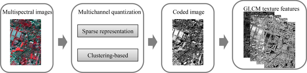
The multichannel images are first processed with the proposed multichannel gray level quantization algorithm, e.g., clustering or sparse representation. The GLCM textural measures are then computed from the quantized images, with window size w × w and displacement vector (δ,θ). The clustering-based GLCM (C-GLCM) textures are called K-means GLCM and FCM GLCM, corresponding to the two clustering algorithms. The sparsity-based algorithms for the GLCM texture extraction from multi/hyperspectral image are called S-GLCM (1) and S-GLCM (2), related to the two different rules which transfer the sparse dictionary to the quantization levels.
A graphical example is shown in Figure 1 to demonstrate the proposed multichannel GLCM texture calculation.
4. Experiments and Analysis
4.1. Datasets and Parameters
In order to validate the effectiveness of the proposed multichannel GLCM algorithms for texture feature representation and the classification of multi/hyperspectral imagery, experiments were conducted on four test images: GeoEye-1 and QuickBird multispectral images of the city of Wuhan, the well-known AVIRIS hyperspectral dataset from the Indian Pines test site, and the HYDICE airborne hyperspectral dataset from the Washington DC Mall. The texture measures of GLCM adopted in this study are: energy (ENE), contrast (CON), entropy (ENT), and (INV). These measures are calculated by setting the inter-pixel distance of one in four directions (0°, 45°, 90°, 135°), and, subsequently, the directionality is suppressed by averaging the extracted features over the four directions. Considering the multi-scale characteristics of the land-cover classes in remote sensing imagery, the experiments were performed with multiple window sizes: 3 × 3, 5 × 5, …, 29 × 29, with four different quantization levels (8, 16, 32, 64). In addition, the GLCM texture features were also extracted from the first principal component of the multi/hyperspectral images and all the original multispectral bands, for the purpose of comparison, which are referred to PCA-GLCM and All-GLCM in the following text, respectively. Moreover, the GLCM texture features extracted from clustering and sparse strategies were combined (called C&S-GLCM in the following text) in order to test whether their integration can further improve the classification accuracy. In the experiments, the extracted GLCM texture features stacked with the spectral bands were classified via the SVM classifier. SVM was implemented by the use of a Gaussian radial-basis function (RBF) kernel. The penalty parameter and the bandwidth of the RBF kernel were selected by fivefold cross-validation [24]. The overall accuracy (OA) and Kappa coefficient were used to evaluate the classification accuracy. Moreover, the statistical significance test, z-score [25], is used to check whether the difference of the classification results obtained by the different algorithms is significant. z > 1.96, −1.96 ≤ z ≤ 1.96 and z < −1.96 denote positive, no, and negative statistical significance, respectively. In addition, the computation time for the considered algorithms is reported.
4.2. Results and Analysis
4.2.1. GeoEye-1 Wuhan Data
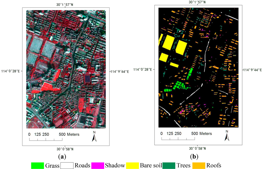
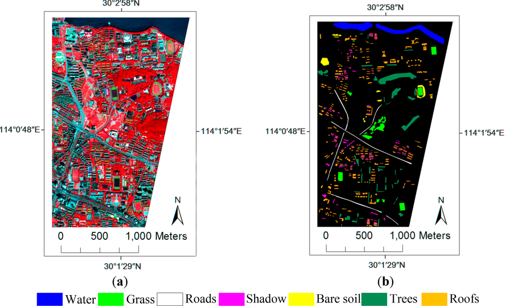
The Wuhan GeoEye-1 test image, with 908 × 607 pixels in four spectral bands (red, green, blue, and near-infrared) and a 2.0-m spatial resolution, is shown in Figure 2a. The information for the ground truth reference is shown in Figure 2b and Table 2. The training (100 pixels for each class) samples were randomly selected from the reference image and the remainder composed the test set.
The classification accuracies achieved by the different texture extraction algorithms with their optimal parameters and the corresponding computation time are compared in Table 3. The z-scores used to compare the classification results between the proposed methods and the traditional PCA-GLCM are also provided. From Table 3, we can obtain the following observations:
- (a)
The accuracy of the spectral classification is significantly improved by introducing the textural features, and the increments in the OA are 13.6%∼16.8%.
- (b)
The proposed multichannel GLCM algorithms, including both the clustering-based (C-GLCM) and sparsity-based (S-GLCM) methods, outperform the traditional PCA-GLCM, with less computation time. Furthermore, this conclusion is also supported by the significance test (z > 1.96). Meanwhile, the proposed S-GLCM algorithms give better result than the All-GLCM. It is worth mentioning that the S-GLCM algorithms give better results than the C-GLCM, with an increment of 2.1% for the OA.
- (c)
The sparsity-based GLCM can obtain satisfactory results with only 8-level quantization. This infers that the sparse approach is able to efficiently represent the multispectral images.
In order to test the robustness of the proposed algorithms, the average accuracies of each technique over the 14 window sizes and four quantization levels are compared in Table 4. It can be seen that the proposed C-GLCM, S-GLCM, C&S-GLCM outperform the traditional PCA-GLCM, and the increments in the average accuracy are 1.4%∼3.7%. In addition, the S-GLCM algorithms give better result than the All-GLCM by an average increment of 2%. The C-GLCM algorithms achieve similar results with the All-GLCM, which outperforms the PCA-GLCM.
The average accuracies of each texture classification algorithm with the various quantization levels are provided in Table 5. It can be clearly observed that the proposed multichannel GLCM algorithms provide more accurate results than PCA-GLCM in all the quantization levels. Furthermore, in general, the two sparse GLCM methods give higher accuracies than the clustering-based GLCM, especially for low quantization levels (e.g., 8, 16). It is interesting to see that when comparing PCA-GLCM and S-GLCM with a quantization level of 8, the improvement in OA achieved by the latter is as high as 10.4%.
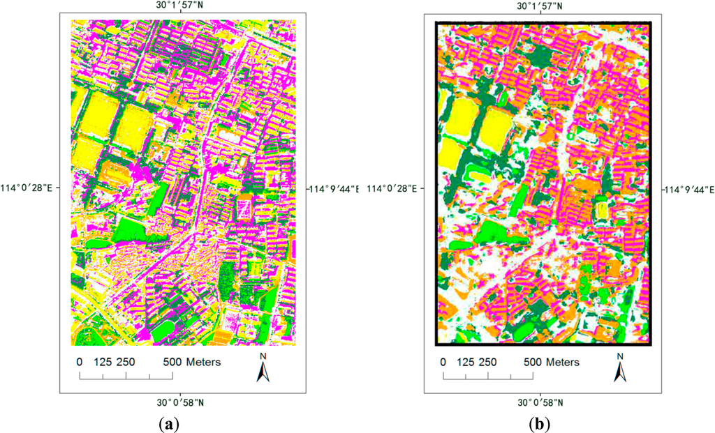
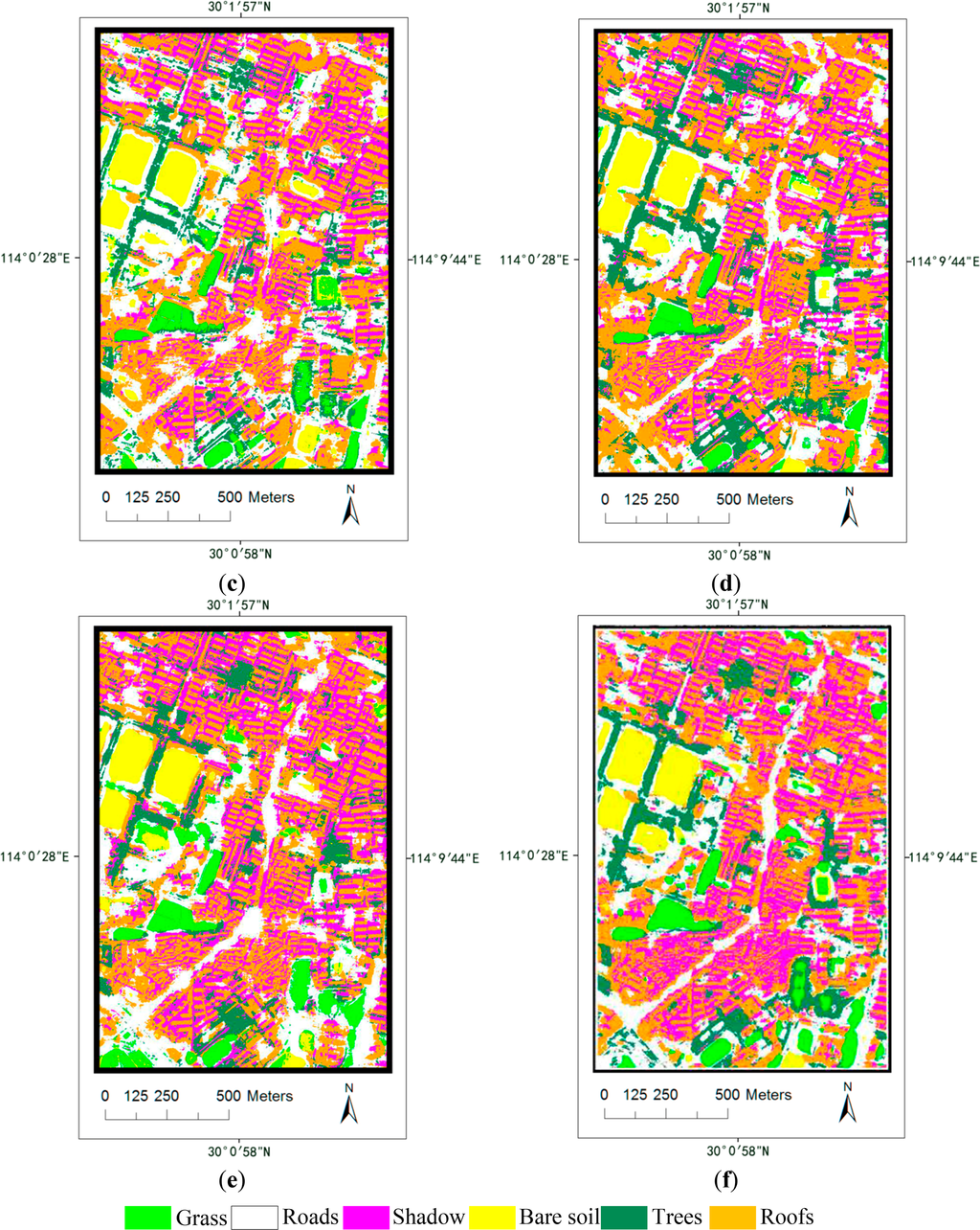
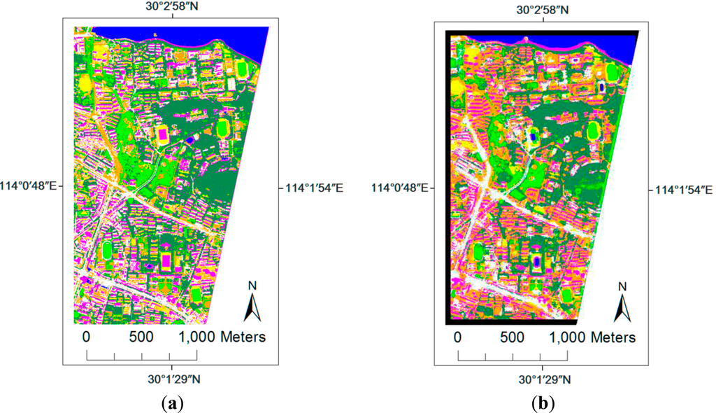
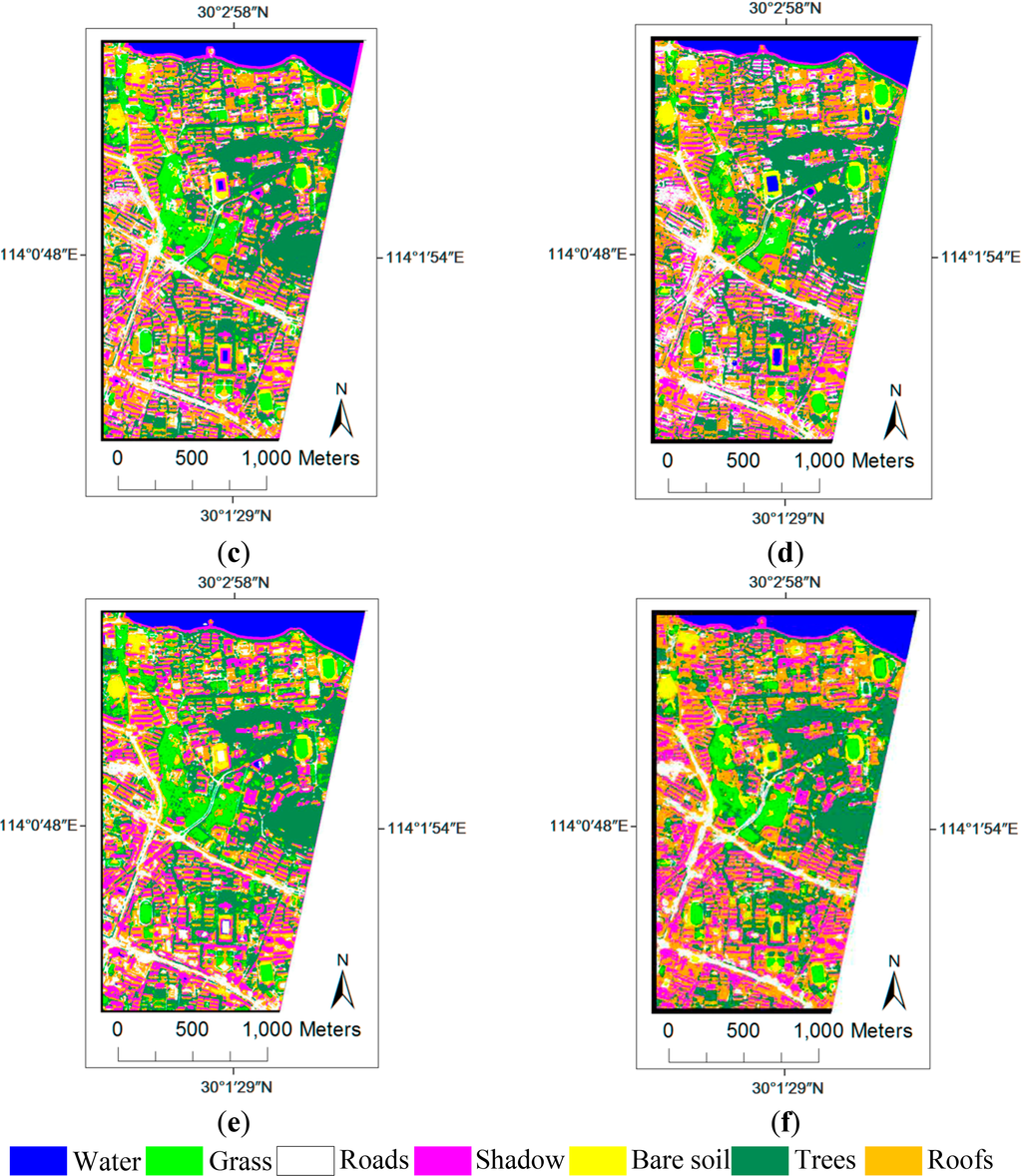
The classification maps of the spectral classification, All-GLCM, PCA-GLCM, the proposed S-GLCM, C-GLCM and C&S-GLCM are compared in Figure 3, for a visual inspection.
4.2.2. QuickBird Wuhan Data
In this case, a QuickBird multispectral image of Wuhan city was also used to validate the proposed multichannel texture extraction algorithms. The color composite image is shown in Figure 4a, comprising 1123 lines and 748 columns with a spatial resolution of 2.4 m. The information for the reference map is provided in Figure 4b and Table 6. We randomly chose 100 samples for each class from the reference image for training, and the remaining samples composed the test set.
The classification results achieved by the different texture extraction algorithms with their optimal parameters are reported in Table 7, and the classification maps are compared in Figure 5. The classification accuracies based on the original multispectral image are: OA = 87.6% and Kappa = 0.854. By analyzing Table 7, the original spectral classification is substantially improved by taking the textural features into account. In addition, it can be seen that the highest accuracy is achieved by C&S-GLCM (OA = 97.0%), while S-GLCM ranks in the second place. Furthermore, it should be noted that the proposed algorithms give better results than All-GLCM with less computation time. The conclusion is also supported by the significance test with all the z-scores > 1.96, which indicates that the difference of the classification results obtained by the proposed algorithms significantly outperform PCA-GLCM.
The average accuracies of each texture classification algorithm for all the parameters and different quantization levels are presented in Tables 8 and 9, respectively. It can be seen from Table 8 that the proposed algorithms give better results than the traditional PCA-GLCM and All-GLCM, with an increment of 0.5%∼2% in the OA. Moreover, the S-GLCM and C&S-GLCM strategies give the best accuracies. From the results in Table 9, it can be seen that S-GLCM, C-GLCM, and C&S-GLCM achieve higher accuracies than PCA-GLCM and All-GLCM in all the quantization levels.
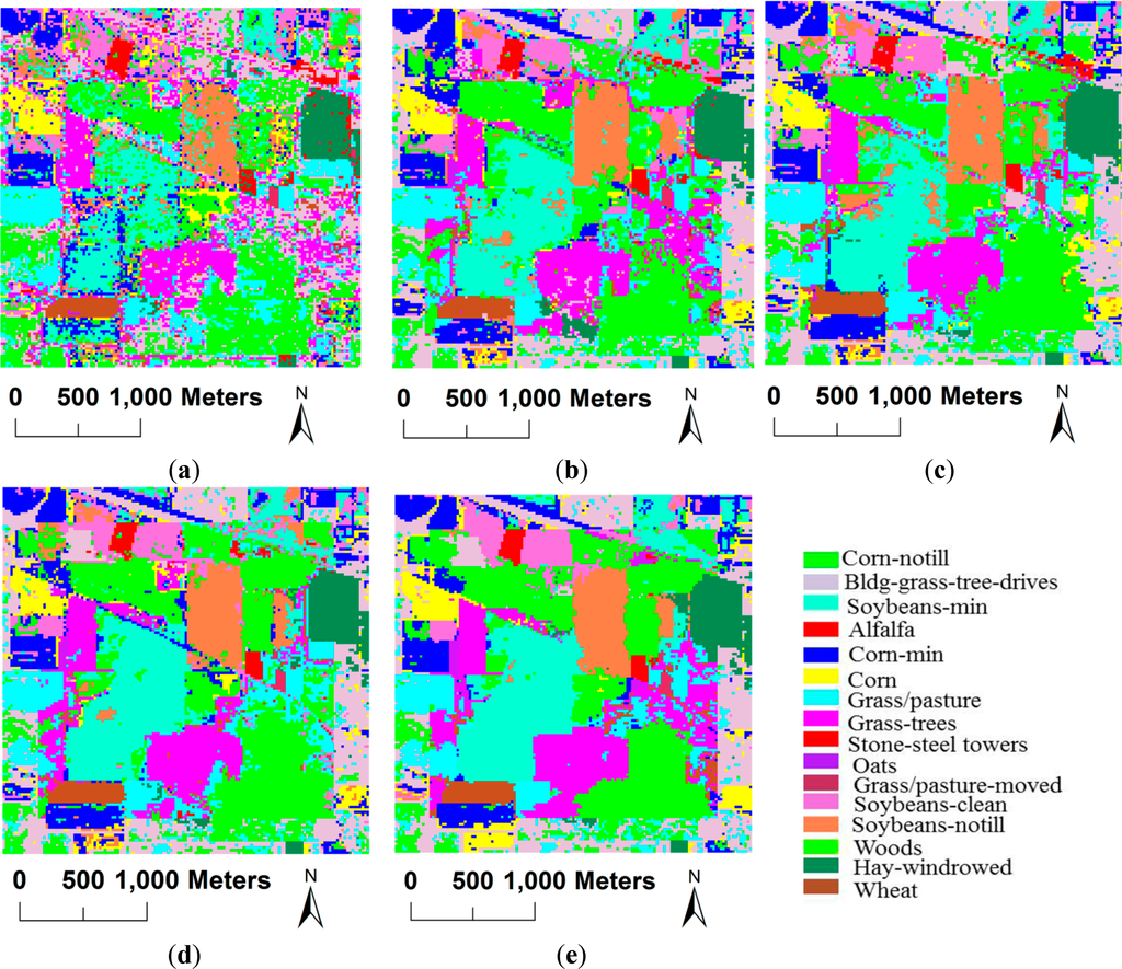
4.2.3. AVIRIS Indian Pines Dataset
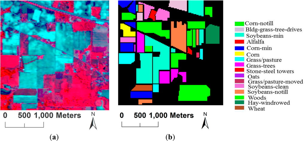
The proposed algorithms were further tested with the AVIRIS hyperspectral dataset from the Indian Pines test site. This image comprises 145 lines and 145 columns, with a spatial resolution of 20 m/pixel and 220 bands. The reference image contains 16 classes, representing various types of crops (Table 10). The RGB image and the reference image are shown in Figure 6. We randomly chose 50 samples for each class from the reference image for training, except for the classes of “alfalfa”, “grass/pasture-mowed”, “oats”, and “stone-steel towers”. These classes contain a limited number of samples in the reference data, and, hence, only 15 samples for each class were chosen randomly for training. The remaining samples composed the test set.
The classification results achieved by the different texture extraction algorithms with their optimal parameters are listed in Table 11. The classification maps of the different feature combinations are compared in Figure 7. In this dataset, the spectral-only classification cannot effectively discriminate between different information classes, resulting in an OA of only 68.2%. The exploitation of the GLCM textures can significantly improve the results, regardless of the specific GLCM texture extraction algorithm, and the increments of the OA are 12.8%∼19.4%. It can be seen from Table 11 that both the clustering-based (C-GLCM) and sparsity-based (S-GLCM) methods outperform the original PCA-GLCM, with a 2.1%∼3.6% increment in OA. In particular, the C&S-GLCM gives higher accuracy than PCA-GLCM by about 6.6%. The z-scores from Table 11 also verified the above observations.
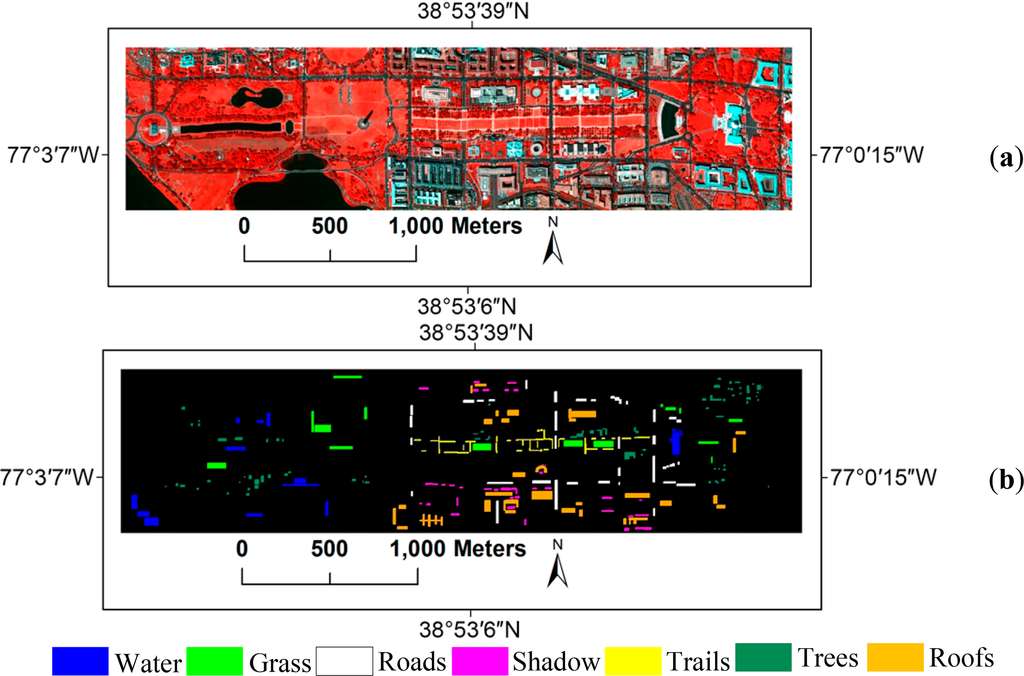
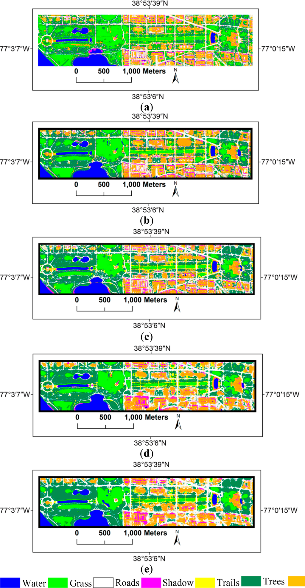
4.2.4. HYDICE DC Mall Dataset
In this experiment, the well-known HYDICE airborne hyperspectral dataset over the Washington DC Mall was used for evaluation of the proposed algorithms. This image comprises 1280 lines and 307 columns, with a spatial resolution of 3 m/pixel and 191 bands. The testing images and the reference data are provided in Figure 8 and Table 12. 50 samples for each class are randomly chosen from the reference image for training, and the remaining samples compose the test set.
The classification results achieved by the different texture extraction algorithms with their optimal parameters are reported in Table 13, and the classification maps are compared in Figure 9. From the table, it can be seen that both the clustering-based (C-GLCM) and sparsity-based (S-GLCM) methods outperform the original PCA-GLCM, with a 2.2%∼2.6% increment in OA. Meanwhile, the C&S-GLCM gives higher accuracy than PCA-GLCM by 3.7%. The conclusion is also supported by the significance test since all the proposed multichannel GLCM methods have the z-scores larger than 1.96 compared to the PCA-GLCM.
4.2.5. Discussion
Some important issues for the proposed methods and the experimental results are discussed below.
- (1)
Accuracies: The proposed multichannel GLCM methods can provide accurate classification results for both multispectral and hyperspectral images, by exploiting the synthesized texture information from multi/hyperspectral bands. Compared to the original spectral classification, the accuracy increments achieved by the optimal multichannel textures are 16.8%, 9.4%, 19.4%, and 9.0%, respectively, for the GeoEye-1, QuickBird, AVIRIS, and HYDICE images.
- (2)
Comparison: The traditional texture extraction methods from multi/hyperspectral remote sensing images are based one of the spectral bands [7,8], panchromatic band [9,12], or the first component of PCA images [10]. In this study, we compared the proposed multichannel GLCM and the PCA-GLCM. It can be found that the proposed methods significantly outperformed the traditional PCA-GLCM in terms of the significance test. This phenomenon can be attributed to the fact that the proposed methods can consider the contributions of multi/hyperspectral bands to the texture representation more effectively.
- (3)
Uncertainties: A possible uncertainty for the proposed method refers to the selection of parameters, including the window size and quantization level. From the Tables 3, 7, 11, and 13, it can be seen that the optimal quantization levels are different for different methods. However, it can be noticed that 8-level quantization (Ng = 8) is appropriate for sparsity-based strategy, since most of the best accuracies for the sparsity-based GLCM were given by Ng = 8. With respect to the window size, no clear regularity can be observed. The suitable window size should be tuned according to the spatial resolution of an image and the characteristics of the objects in the image.
5. Conclusions
The traditional GLCM (Gray Level Co-occurrence Matrix) texture is calculated based on a mono-spectral image, e.g., one of the multispectral bands, the first principal component, or the panchromatic image. In this study, we propose a novel multichannel GLCM texture feature representation for multi/hyperspectral images, based on a series of image coding methods. The motivation of this study is to more effectively represent the texture information from multi/hyperspectral images.
Specifically, clustering and sparse representation techniques are adopted to generate codes or quantized levels for the multichannel texture extraction. It should be noted that although the sparse representation methods have been applied in computer vision and pattern recognition, few studies have been reported concerning their application in texture analysis.
The experiments were conducted on four multi/hyperspectral datasets. The optimal overall accuracies (OA) achieved by the proposed multichannel GLCM methods are satisfactory. With the multispectral datasets, 91.5% and 97.0% accuracy scores were obtained for the GeoEye-1, and QuickBird images, respectively. With respect to the hyperspectral datasets, 87.6% and 98.8% for the overall accuracy (OA) were given, respectively, for the AVIRIS and HYDICE images. The experimental results verify that the proposed sparse GLCM (S-GLCM) outperforms the traditional PCA-GLCM in terms of the classification accuracies and significance test. It is also found that the S-GLCM achieves slightly better results than the clustering-based GLCM (C-GLCM). Considering that most of the remote sensing applications are related to multi/hyperspectral images, the proposed multichannel texture extraction strategies could be included as one of the standard feature extraction tools.
A possible direction for the future research is to extend the proposed strategy to other texture measures, e.g., multichannel local binary pattern (LBP). We also plan to focus our research on the texture extraction from hyperspectral data, which has high-dimensional and sparse spectral space.
Acknowledgments
The authors would like to thank the editor and the anonymous reviewers for their comments and suggestions. This research is supported by the National Natural Science Foundation of China under Grants 41101336 and 91338111, the Program for New Century Excellent Talents in University of China under Grant NCET-11-0396, and the Foundation for the Author of National Excellent Doctoral Dissertation of PR China (FANEDD) under Grant 201348.
Author Contributions
Xin Huang proposed the idea of the multichannel texture extraction method, and organized the writing and revision of the paper. Xiaobo Liu contributed to the programming and experiments, and drafted the manuscript. Liangpei Zhang provided advice for preparing and revising the paper.
Conflicts of Interest
The authors declare no conflict of interest.
References
- Kitada, K.; Fukuyama, K. Land-use and Land-cover mapping using a gradable classification method. Remote Sens 2012, 4, 1544–1558. [Google Scholar]
- Racoviteanu, A.; Williams, M.W. Decision tree and texture analysis for mapping debris-covered glaciers in the Kangchenjunga area, eastern Himalaya. Remote Sens 2012, 4, 3078–3109. [Google Scholar]
- Myint, S.W.; Lam, N.S.N.; Tyler, J.M. Wavelets for urban spatial feature discrimination: Comparisons with fractal, spatial autocorrelation, and spatial co-occurrence approaches. Photogramm. Eng. Remote Sens 2004, 70, 803–812. [Google Scholar]
- Dell’Acqua, F.; Gamba, P.; Ferrari, A.; Palmason, J.A.; Benediktsson, J.A.; Arnason, K.A.A.K. Exploiting spectral and spatial information in hyperspectral urban data with high resolution. IEEE Geosci. Remote Sens. Lett 2004, 1, 322–326. [Google Scholar]
- Haralick, R.M.; Shanmugam, K.; Dinstein, I.H. Textural features for image classification. IEEE Trans. Syst. Man Cybern 1973, 6, 610–621. [Google Scholar]
- Zhang, Y. Optimisation of building detection in satellite images by combining multispectral classification and texture filtering. ISPRS J. Photogramm. Remote Sens 1999, 54, 50–60. [Google Scholar]
- Franklin, S.E.; Peddle, D.R. Classification of SPOT HRV imagery and texture features. Int. J. Remote Sens 1990, 11, 551–556. [Google Scholar]
- Gong, P.; Marceau, D.J.; Howarth, P.J. A comparison of spatial feature extraction algorithms for land-use classification with SPOT HRV data. Remote Sens. Environ 1992, 40, 137–151. [Google Scholar]
- Puissant, A.; Hirsch, J.; Weber, C. The utility of texture analysis to improve per-pixel classification for high to very high spatial resolution imagery. Int. J. Remote Sens 2005, 26, 733–745. [Google Scholar]
- Zhang, L.; Huang, X.; Huang, B.; Li, P. A pixel shape index coupled with spectral information for classification of high spatial resolution remotely sensed imagery. IEEE Trans. Geosci. Remote Sens 2006, 44, 2950–2961. [Google Scholar]
- Huang, X.; Zhang, L.; Li, P. Classification and extraction of spatial features in urban areas using high-resolution multispectral imagery. IEEE Geosci. Remote Sens. Lett 2007, 4, 260–264. [Google Scholar]
- Pacifici, F.; Chini, M.; Emery, W.J. A neural network approach using multi-scale textural metrics from very high-resolution panchromatic imagery for urban land-use classification. Remote Sens. Environ 2009, 113, 1276–1292. [Google Scholar]
- Lucieer, A.; Stein, A.; Fisher, P. Multivariate texture-based segmentation of remotely sensed imagery for extraction of objects and their uncertainty. Int. J. Remote Sens 2005, 26, 2917–2936. [Google Scholar]
- Palm, C. Color texture classification by integrative co-occurrence matrices. Pattern Recognit 2004, 37, 965–976. [Google Scholar]
- Palm, C.; Lehmann, T.M. Classification of color textures by gabor filtering. Mach. Graph. Vis 2002, 11, 195–219. [Google Scholar]
- Rao, C.N.; Sastry, S.S.; Mallika, K.; Tiong, H.S.; Mahalakshmi, K.B. Co-occurrence matrix and its statistical features as an approach for identification of phase transitions of mesogens. Int. J. Innov. Res. Sci. Eng. Technol 2013, 2, 4531–4538. [Google Scholar]
- Clausi, D.A. Comparison and fusion of co-occurrence, Gabor and MRF texture features for classification of SAR sea-ice imagery. Atmos. Ocean 2001, 39, 183–194. [Google Scholar]
- Celebi, M.E.; Kingravi, H.A.; Vela, P.A. A comparative study of efficient initialization methods for the k-means clustering algorithm. Expert Syst. Appl 2013, 40, 200–210. [Google Scholar]
- Kaur, P.; Soni, A.K.; Gosain, A. A robust kernelized intuitionistic fuzzy c-means clustering algorithm in segmentation of noisy medical images. Pattern Recognit. Lett 2013, 34, 163–175. [Google Scholar]
- Lee, H.; Battle, A.; Raina, R.; Ng, A.Y. Efficient sparse coding algorithms. Adv. Neural Inf. Process. Syst 2007, 19, 801. [Google Scholar]
- Aharon, M.; Elad, M.; Bruckstein, A. The K-SVD: An algorithm for designing of overcomplete dictionaries for sparse representations. IEEE Trans. Signal Process 2006, 54, 4311–4322. [Google Scholar]
- Mairal, J.; Bach, F.; Ponce, J.; Sapiro, G. Online learning for matrix factorization and sparse coding. J. Mach. Learn. Res 2010, 11, 19–60. [Google Scholar]
- Tibshirani, R. Regression shrinkage and selection via the lasso. J. R. Stat. Soc. Ser. B (Method) 1996, 58, 267–288. [Google Scholar]
- Chang, C.-C.; Lin, C.-J. LIBSVM: A library for support vector machines. ACM Trans. Int. Syst. Technol 2011, 2, 1–27. [Google Scholar]
- Foody, G. Thematic map comparison: Evaluating the statistical significance of difference in classification accuracy. Photogramm. Eng. Remote Sens 2004, 70, 627–633. [Google Scholar]
© 2014 by the authors; licensee MDPI, Basel, Switzerland This article is an open access article distributed under the terms and conditions of the Creative Commons Attribution license (http://creativecommons.org/licenses/by/3.0/).