An Alternative Approach to Mapping Thermophysical Units from Martian Thermal Inertia and Albedo Data Using a Combination of Unsupervised Classification Techniques

Abstract

Thermal inertia and albedo provide information on the distribution of surface materials on Mars. These parameters have been mapped globally on Mars by the Thermal Emission Spectrometer (TES) onboard the Mars Global Surveyor. Two-dimensional clusters of thermal inertia and albedo reflect the thermophysical attributes of the dominant materials on the surface. In this paper three automated, non-deterministic, algorithmic classification methods are employed for defining thermophysical units: Expectation Maximisation of a Gaussian Mixture Model; Iterative Self-Organizing Data Analysis Technique (ISODATA); and Maximum Likelihood. We analyse the behaviour of the thermophysical classes resulting from the three classifiers, operating on the 2007 TES thermal inertia and albedo datasets. Producing a rigorous mapping of thermophysical classes at ~3 km/pixel resolution remains important for constraining the geologic processes that have shaped the Martian surface on a regional scale, and for choosing appropriate landing sites. The results from applying these algorithms are compared to geologic maps, surface data from lander missions, features derived from imaging, and previous classifications of thermophysical units which utilized manual (and potentially more time consuming) classification methods. These comparisons comprise data suitable for validation of our classifications. Our work shows that a combination of the algorithms—ISODATA and Maximum Likelihood—optimises the sensitivity to the underlying dataspace, and that new information on Martian surface materials can be obtained by using these methods. We demonstrate that the algorithms used here can be applied to define a finer partitioning of albedo and thermal inertia for a more detailed mapping of surface materials, grain sizes and thermal behaviour of the Martian surface and shallow subsurface, at the ~3 km scale.

1. Introduction

The materials exposed at the surface of Mars are varied in composition and are found in a range of states of aggregation. Dust, sandy soils and sediments, pebbles, and rocks, are globally distributed, have been observed over three decades of orbiter missions to Mars, and have been analysed and characterised at outcrop scale by lander instrumentation. Detailed mapping of the distribution and spatial variation of Mars’s surface materials is a necessary and important task. The distribution of materials needs to be known when planning for the selection of landing sites, due to: (a) engineering requirements for landing instrumentation; and, (b) the selection of sites of scientific interest. Determination of rock-size frequencies is essential for evaluating safety in the landing and operations of rovers [1]. It is important to avoid landing in terrains covered by thick layers of dust or loose sediments as landing locations must be selected to include outcrops of geological significance to collect scientific data [2]. Knowledge of the spatial variation of surface materials is also significant from a purely scientific viewpoint, because what is presently observed represents a snapshot of the geological and atmospheric processes which occurred in the recent past. While Martian dust particles of dimensions of ~1–10 μm remain in suspension indefinitely [3], larger grains of dust and silt (diameter: 60 μm) are lifted, carried in Mars’s atmosphere, and eventually fall out and become part of the Martian soil. Larger grained materials, such as sand particles (up to a few hundred μm in size) may be moved by saltation [4] and, upon breaking, may be lifted and carried over large distances by the atmospheric currents. Larger particles (such as coarse grained sand and hematite concretions up to 1–5 mm) may move only short distances by drag, but usually accumulate as lag deposits [5,6]. Consequently, the mineralogical and chemical characterisation of materials evaluated against their particle sizes, provides insights about the provenance of the material, leading to valuable geological inference.

Other than from direct measurements of grain dimensions of minerals within an outcrop (e.g., by Microscopic Imager onboard Mars Exploration Rovers Spirit and Opportunity), the best knowledge of the distribution of surface materials and their size frequencies arises from estimates of their physical properties from remote-sensing data. Martian global dust is characterised by low values of thermal inertia and high values of albedo. Vice-versa, high values of thermal inertia and low albedo are typical of rock and duricrust [2]. Intermediate values of these physical properties however cannot be readily interpreted [7]. Therefore, previous authors (e.g., [8]) have applied a supervised pixel classification method to measurements of thermal inertia and albedo acquired by the Thermal Emission Spectrometer (TES) on board the Mars Global Surveyor orbiter. Their work resulted in a map of surface materials subdivided into seven broad classes [8,9]. Of these, three were clearly characterised: (A) low TI-high albedo, corresponding to unconsolidated fines; (B) high TI-low albedo, corresponding to (mostly) sand, rock and bedrock; (C) high TI-medium albedo, corresponding to (mostly) duricrust. The remaining four classes (D–G) represented outliers in the values of TI and albedo, of uncertain interpretations. In a follow-up paper, the effects of horizontal mixtures and layering of two end-members, as well as slope, were modelled [10], with the resulting 5° resolution thermophysical maps showing the prevalent effect of layering at mid-latitudes and in the polar regions, with less common and more localized horizontal mixing and slope effects.

As shown in

Table 1. Characteristics of primary Martian surface materials, reproduced from [11].

Material	Dimensions (Grain Size) *	Thermal Inertia (tiu)	Albedo	Diurnal Skin Depth (cm) **	Refs. ***
Dust	2–60 μm	20–150	>0.27	0.3–2.5	[12–17]
Sand	60–2000 μm	150–400	<0.15	2.5–6.7	[9,18,19]
Duricrust	Grains 100–300 μm Bulk 0.6–3 mm	350–600	<0.15	5.9–10.1	[14,16–18,20–22]
Granules/very coarse sand	2–4 mm	400–800	<0.15	6.7–13.5	[9,14,17,18,22]
Pebbles/rocks/bedrock	4–250 mm	800–2068	<0.15	13.5–34.8	[14,22–26]
Boulders/ice-cemented soil	>250 mm	>2068	<0.1	>34.8	[1,14,22,27]
Ice		>2500	>0.4	>42.1	[28,29–31]

^*Grain size classified according to the Wentworth scale [32].

^**Calculated using: product of density and specific heat on the Martian surface of ~10⁶ J/m³/K [33]; Martian diurnal period value of 8.9 × 10⁴ s; I values given in table.

^***The values for each material are derived from a combination of remote sensing and laboratory data.

, combinations of thermal inertia (TI) and albedo can discriminate Martian materials ([12–33]). In-situ investigations by rover instruments Mini-TES (Miniature Thermal Emission Spectrometer) and MI (Microscopic Imager) at Meridiani Planum (Opportunity; e.g., [5,6,34,35]) and Gusev Crater (Spirit; e.g., [6,35–37]), and ChemCam at Gale Crater (Curiosity; e.g., [38–40]), have unveiled a rich variety of surface materials of variable size and state of aggregation. These include bedrock, rocks, pebbles, loose sediments, dust, compacted sediments, hollow-filling sediments, boulders and duricrust. Compositional differences also exist. For example, in Gale crater both a fine-grained soil of mafic composition and a coarse-grained soil of felsic composition were detected along a Curiosity transect, with the latter appearing to be locally derived [39], and the former akin to global Mars mafic dust [39,41]. Mafic soils similar in composition to Martian dust were also observed by Spirit and Opportunity (e.g., [42,43]).

Thermal inertia and albedo provide a means of probing the physical properties of shallow subsurface materials which may be obscured by thermally thin coverings of dust and particulates. Examples of applications are: searching for obscured bedrock and thermally distinct units (e.g., floors of paleolakes [44]); identifying near-surface ice in lobate debris aprons and pingoes (e.g., [45]); and modeling regional ice stability and permafrost depth [28]. In addition, thermophysical properties of the surface provide necessary inputs to GCM atmospheric circulation models [46], and are still applied as an early criteria in landing site selection [47]. Improving the understanding of the thermophysical properties of the Martian surface at the ~3 km resolution of the Thermal Emission Spectrometer (TES) remains scientifically valuable, despite the availability of thermal inertia values at ~100 m/pixel resolution from the Thermal Emission Imaging System (THEMIS) [48]. Previous maps of thermophysical units (e.g., [8,49]) remain regularly cited and utilised by the Mars community. Important applications of these global maps are to provide a thermophysical context for spectral and visual observations of the surface and for point measurements (such as in-situ investigations like those at the Phoenix landing site [50]). Data resolution of 3 km is suitable for regional-scale analysis and interpretation, contributing to understanding the relationships between surficial geology, orbital mineralogical features [51–53], and visual morphologies (e.g., slope streaks [54]). Identification of extensive kilometer scale features, such as thermally distinct preserved impact crater ejecta [55], is also an ideal application of thermophysical maps.

This work evaluates unsupervised approaches to mapping thermophysical units. These approaches differ from previous works [7–9,56–58]. All previous thermophysical mappings determined divisions between thermal inertia and albedo units by manually applying thresholds to isolate the strongest peaks and highest pixel densities in the global distribution of thermal inertia and albedo values. Prior mappings were therefore sensitive to the globally-dominant mixtures of material types, particularly those with very high or low albedo and very low thermal inertia, such as bright fine dust, dark sand and bright ice (Table 1).

Table 2. Values of thermal inertia (TI) and albedo that would result in an unambiguous interpretation of surface materials.

TI Threshold	Albedo Threshold	Surface Material Classification	Fraction of Map Pixels %
>1000	<0.15	Rock	0.15
150–400	<0.15	Sand	19.10
<100	>0.25	Dust	12.77
>1000	>0.3	Ice	1.29
		Total:	33.31

presents the values of Martian thermal inertia and albedo that would result in a unique interpretation of a single surface component material dominating the pixel. For example, if a pixel has an orbital thermal inertia of 2000 tiu and an albedo of 0.14, then it can be uniquely interpreted as a rock dominated surface within this classification scheme. The unambiguous values given in Table 2 however occur in only ~33% of pixels in the global map. The remaining ~67% of the map is comprised of more than one surface component. It is not surprising that the majority of the Martian surface is not uniquely classified from orbital thermophysical data, given the heterogeneities discussed above and that each pixel in the thermal inertia and albedo maps encompasses a surface area of ~9 km². This means the separability of classes for a large majority of the Martian surface is inherently low, which makes it important to understand the uncertainties in existing class assignments and the strengths and weaknesses of the manual approaches used in previous studies. The uncertainties associated with manual classifications can be difficult to assess, and previous work assessing the uncertainties in the boundaries between thermophysical classes has been limited. Comparisons with alternative, less deterministic approaches that have been used successfully in terrestrial remote sensing, such as those examined here, can help to address these issues.

Given the complexities inherent with pixel classification of orbiter thermal data, and the importance of thermophysical maps for understanding geological processes on Mars, it is worthwhile to explore alternative classification methods to: (a) corroborate the results of earlier maps and classifications obtained by different techniques; (b) identify any areas of discrepancy; and, (c) interpret new insights deriving from examination of discrepancies. In this work, a comparison of different classification methods is presented, and their ability to improve the classification resolution of Martian thermophysical maps is analysed. The strengths and weaknesses of these new unsupervised approaches are explored, together with examples of applications to specific Martian areas to validate the methods. Some of the factors affecting the sensitivity of the classification algorithms are analysed. The unsupervised classification approach presented here can provide a powerful alternative to manual classification procedures, which are both deterministic in nature and potentially more time consuming. Here we derive and map the geographic distribution of seven Martian thermophysical units, which we discuss by detailed examination of the treatment of the dataspace, and compare them to thermophysical units published in earlier papers [8,9]. The unsupervised classification partitioning of thermophysical units offers new insights in the interpretation of Martian lithologies, stratigraphies, and geological reconstructions. Furthermore, while manual classification techniques are challenging when applied to more than two datasets, the techniques examined here can be utilized on N-dimensions without significantly increased difficulty for the user. This enables their use, for example, in the derivation of multi-dimensional groupings of Martian surface materials characterized through a combination of thermophysical data (albedo and thermal inertia) and mineralogy.

Our work utilizes the 2007 values of thermal inertia which were derived from a large number of seasonal brightness temperature observations from the Thermal Emission Spectrometer and were compiled into an updated thermal inertia map by [10]. The algorithms applied in this work are well documented and are frequently applied to similar classification problems. Gaussian Mixture Models (GMMs) have been shown to provide a good approximation to many diverse data distributions [59–61]. Clustering techniques such as Iterative Self-Organizing Data Analysis Technique (ISODATA) and Maximum Likelihood (MAXLIKE) have been successfully applied to detect the most likely geographic origin of different strains of avian influenza [62] and to characterise galaxy spectra from the Sloan Digital Sky Survey [63], in addition to their usual application to problems related to identification of land cover from remote sensing data sets [64,65]. Two-band classification, for probing the relationship between the red and near infra-red channels, has been of enduring use for investigating surface characteristics across a range of sensors (including Landsat satellites, MODIS and AVHRR, [66]). Many studies have focused explicitly on the relationship between these two bands (e.g., [67–70]), and developing indices for interpreting spectral and land information space. A few studies have also applied algorithmic classification techniques (both supervised and unsupervised) to Martian datasets, including: hyperspectral imagery and mineralogy data from orbital measurements [71–77] and ground-measurements by the rovers [78]; terrain mapping and feature classification from elevation and surface roughness data [79–82] and visual imagery [83]; and automated detection of impact craters [84,85]. The use of algorithmic classification in studies of Mars is increasing over time, however no previous study has applied algorithmic classification to mapping surface grain size and thermal behaviour in Martian thermal inertia and albedo data.

Thermal Inertia & Albedo

Martian thermal inertia and albedo have been discussed in detail by numerous authors and so only a brief description is given here. The data values used in this study are shown in Figure 1. The thermal inertia of a material is a measure of its ability to conduct and store heat [56,86,87]. Thermal insulators (materials with low thermal conductivity) have low thermal inertia, so they rapidly heat and cool at their surface due to their poor ability to distribute heat through conduction into their interior. Thermal inertia values of planetary surfaces are determined by a complex combination of particle size, bedrock outcrop and rock abundance [10], and degree of cementation [7]. Martian albedo is the fraction of incident visible to near-infrared (0.3–2.9 μm) solar radiation reflected by the surface [88]. A combination of both thermal inertia and albedo are needed to understand the thermophysical properties of the surface. Thermal inertia correlates strongly with apparent grain size (particle size and degree of induration, e.g., [12,21]), whereas albedo correlates with mineralogy [15]. Surfaces can display similar orbital thermal inertias, despite significantly different horizontal heterogeneity or vertical layering [10,89]. For example, both the Phoenix and Opportunity landing sites had an apparent thermal inertia of 200 tiu, but could be distinguished through different orbital albedo values of 0.2 and 0.15 respectively (Phoenix [28,50]; Opportunity [35,90,91]). In addition, the subsurface thermal environment is controlled by both parameters, as albedo determines the degree to which solar insolation is absorbed by the surface (bright materials reflect more solar radiation and absorb less heat), and thermal inertia governs the distribution of that heat at depth [7,11].

Global observations by the Thermal Emission Spectrometer (TES), onboard the Mars Global Surveyor, were used to infer the albedo and thermal inertia of the Martian surface. Locally, surface values of these parameters acquired by landers ground-truth the satellite data [92]. The sensing depth of TES is of the order of centimetres at infrared wavelengths, and of millimetres in the visual spectrum [88]. Hence TES provides information only on the shallow subsurface. The resolution of TES is ~3 km/pixel [93,94]. The Martian surface is heterogeneous at this scale, therefore the thermal inertia derived for each pixel represents an integrated radiance and apparent brightness temperature of the surface materials within the satellite’s field of view [1,57].

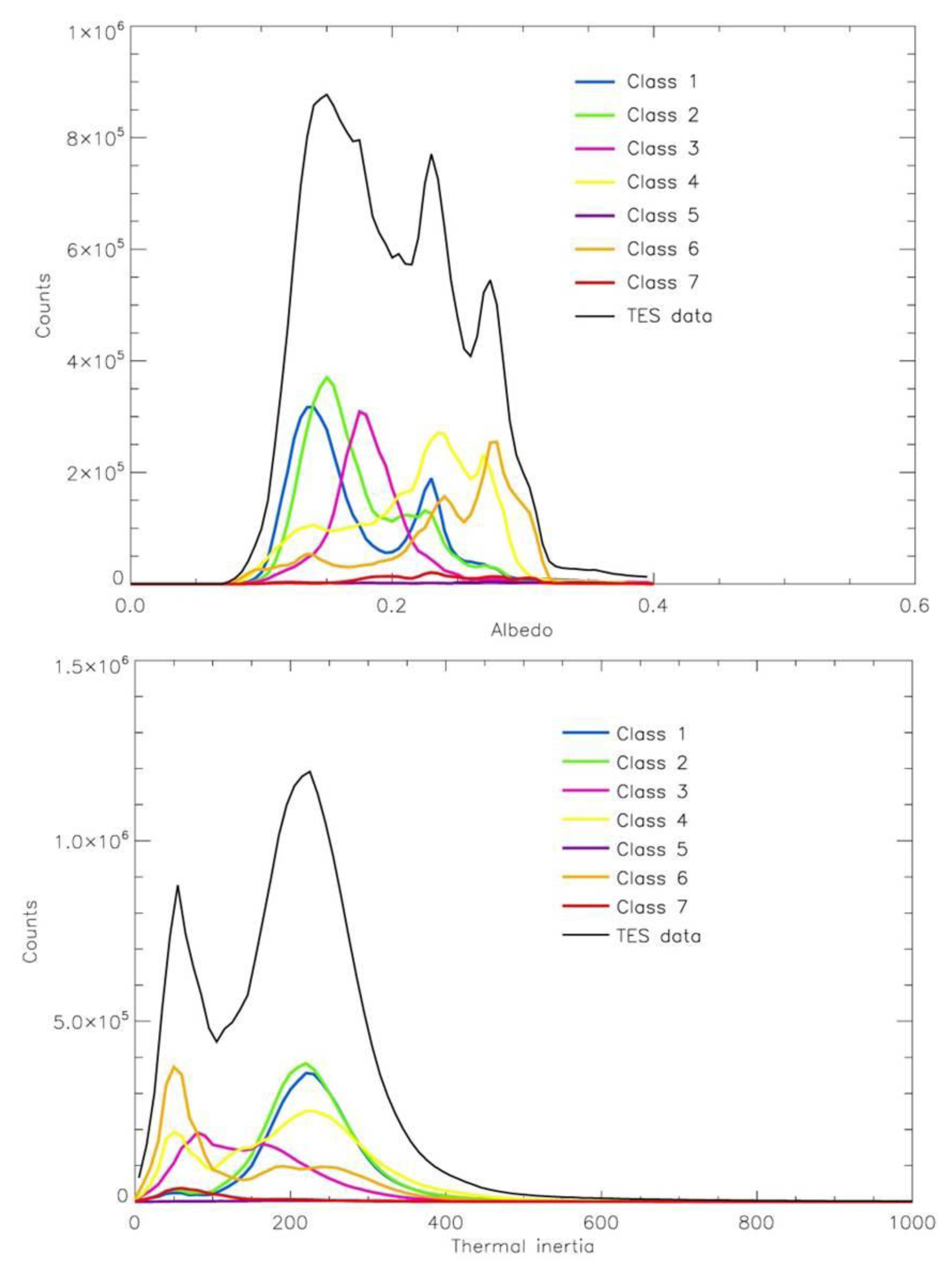
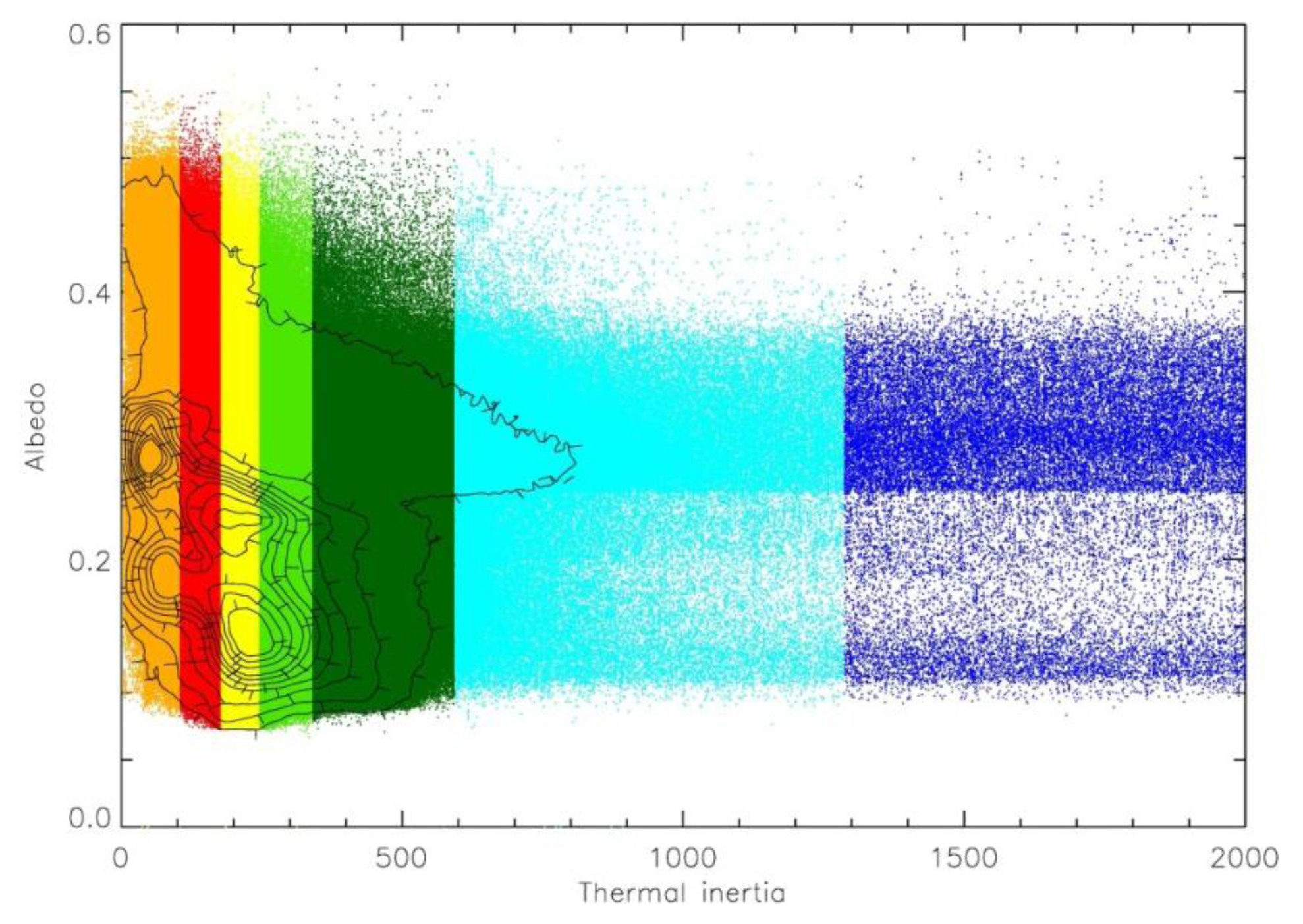
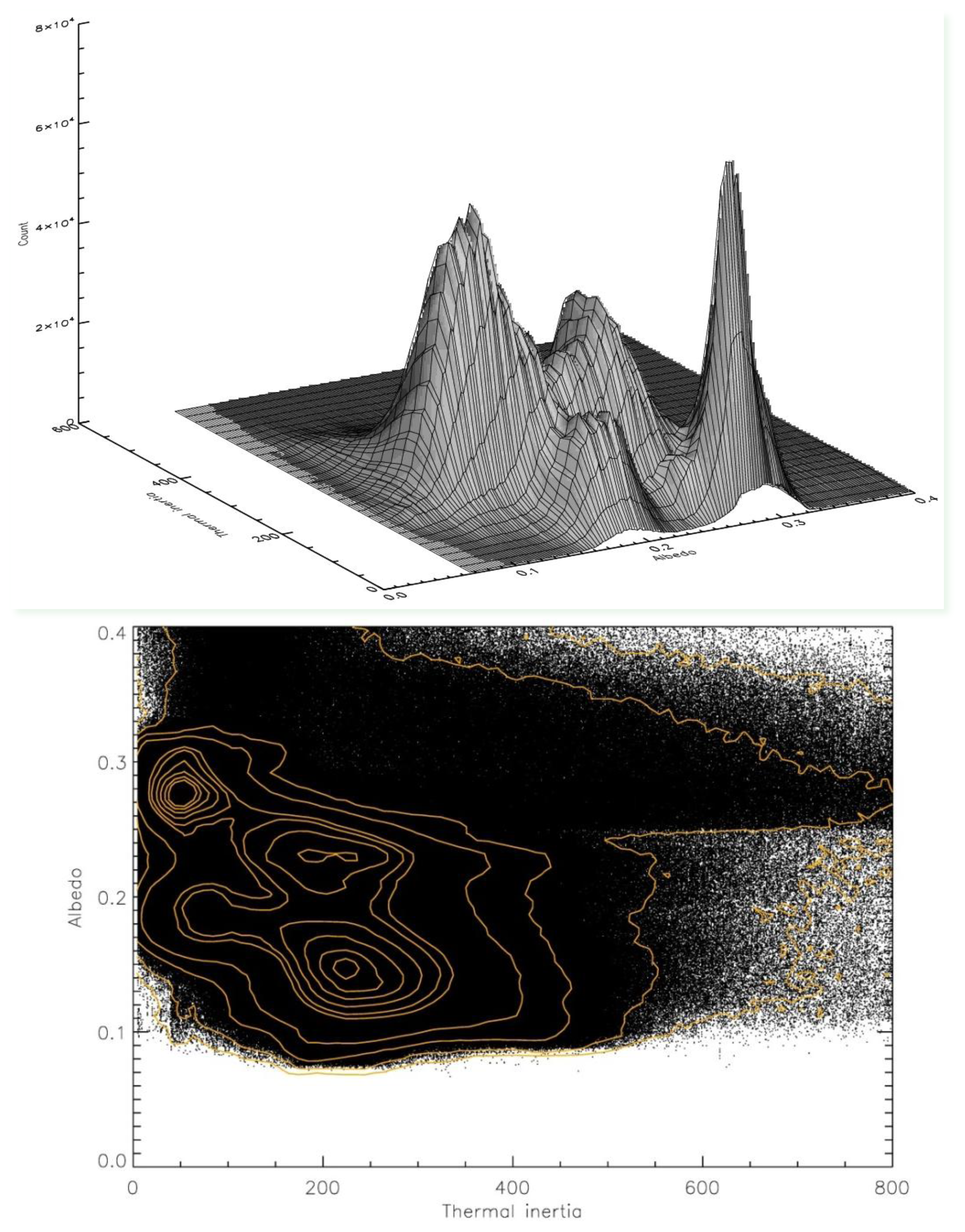
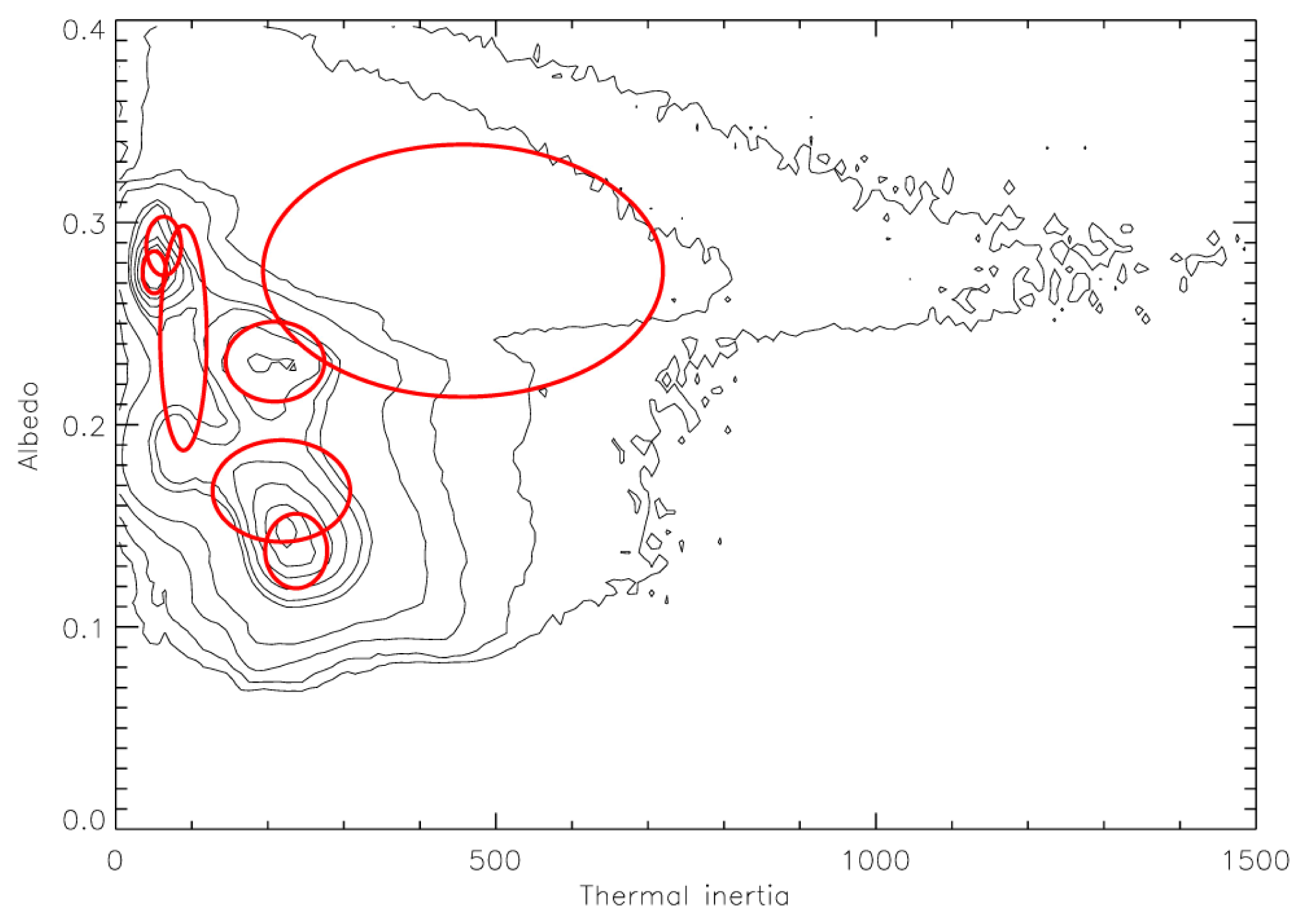
On Mars, high thermal inertia materials (such as rocks) predominantly have lower albedo values than small grained, low thermal inertia materials (such as dust, sand). Bright high albedo regions on Mars indicate fine-grained surface dust, or ice [95,96]. Dark regions correspond to mixtures of sand, rocks, or duricrust (cemented sand sized grains) with smaller proportions of dust. The 3D histogram of Mars’s global albedo and thermal inertia contains four local maxima (Figure 1). One peak is due to the contribution of bright and finely grained dust on the Martian surface (albedo 0.27, thermal inertia 55 J·m⁻²·K⁻¹·s^−1/2 hereafter, tiu). The remainder include contributions from a range of materials of varying grain sizes, including sand, rocks, and duricrust. A scatterplot of global thermal inertia and albedo values on Mars (Figures 1 and 2) reveals the complex relationship between these variables. The classification results presented in this work will be compared to these plots to determine their sensitivity to the major groupings within the two-dimensional albedo-thermal inertia dataspace.

2. Data

The procedure used to determine thermal inertia and albedo using the TES data and the technical details of the TES experiments have been widely published (for example, [7,8,10,56,88]). Additional details of the data are given in Appendix.

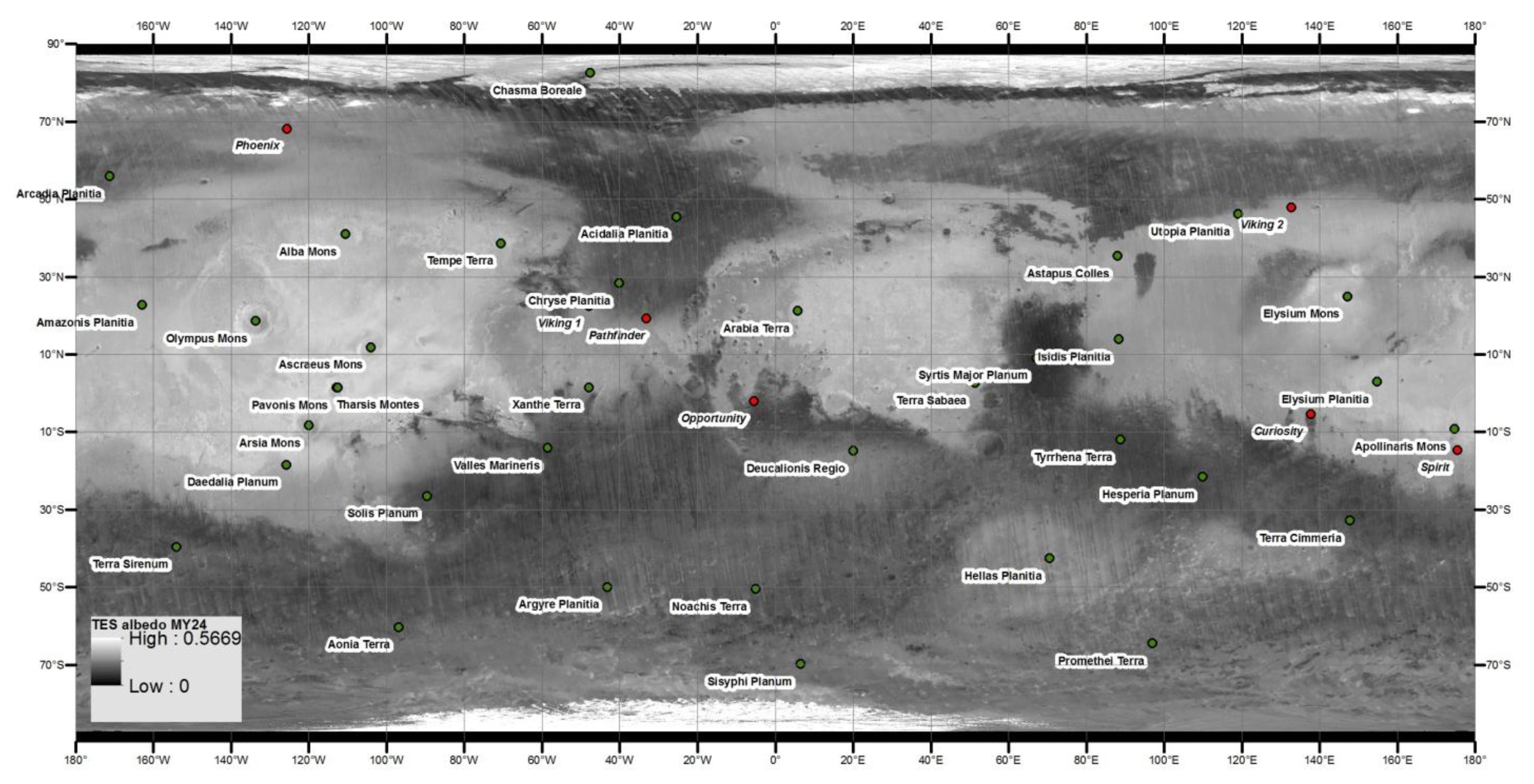
The albedo measurements used here were taken within Martian year MY24, which was characterised by minimal localised dust storm events [97], and a lower dust optical depth (the atmosphere was more transparent) than in MY25 and MY26 [98,99]. The albedo values in MY24 should thus be the most representative of the mean surface materials, being least affected by scattering due to atmospheric dust. The variability in albedo values over MY24 to MY26 was less than ± 0.06 over the vast majority of the Martian surface [10]. This albedo dataset differs from that utilized by [8], which incorporated data from MY25 in the albedo map. The instrument uncertainty in albedo values is approximately ±0.01 [88]. Orbital measurements comprise ~35% (global coverage) of the albedo map [100]. Although observations comprise a small fraction of the albedo map, it overlaps well with the time period during which the thermal inertia mapping occurred.

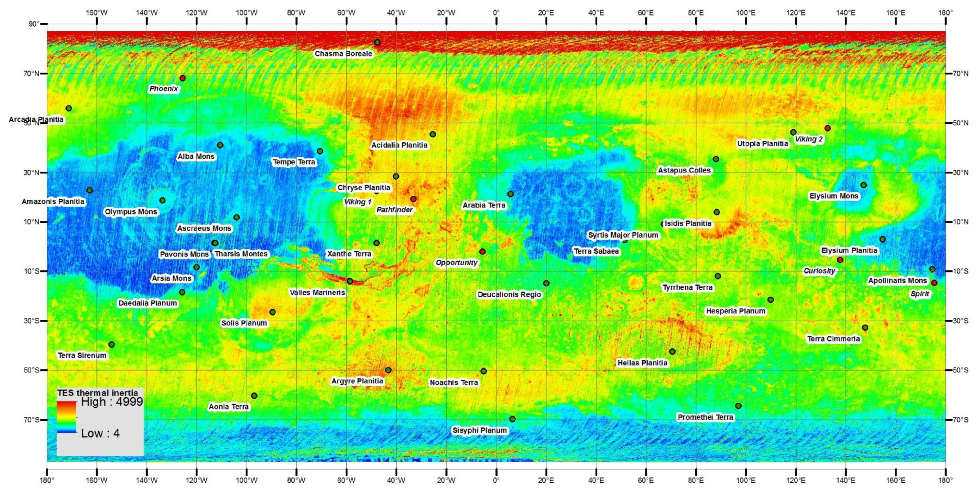
The TES thermal data used to produce the 2007 nightside bolometric thermal inertia dataset [10] (Figure 3) were taken over MY24-27. Data affected by high dust opacity was removed. The nightside map is comprised predominantly of local night-time values, but includes some daytime values in the polar regions [10]. Uncertainties are a combination of instrument measurement error, uncorrected atmospheric effects, and uncertainties in the thermal model. Computational uncertainty in night-time bolometric thermal inertia is estimated to be <10%, and the nightside map values used here may include another <10% error from the other datasets incorporated into the interpolation scheme used to derive thermal inertia (e.g., albedo and dust opacity) and physics not included in the model [10]. The thermal inertia values are the medians of 36 maps of data obtained across the four Martian years, extending from ± 87° (due to the orbital inclination of the spacecraft). Observations constitute ~93% of the map, as it includes a larger number of seasonal observations and incorporate data from more Martian years than the albedo map used here [101]. 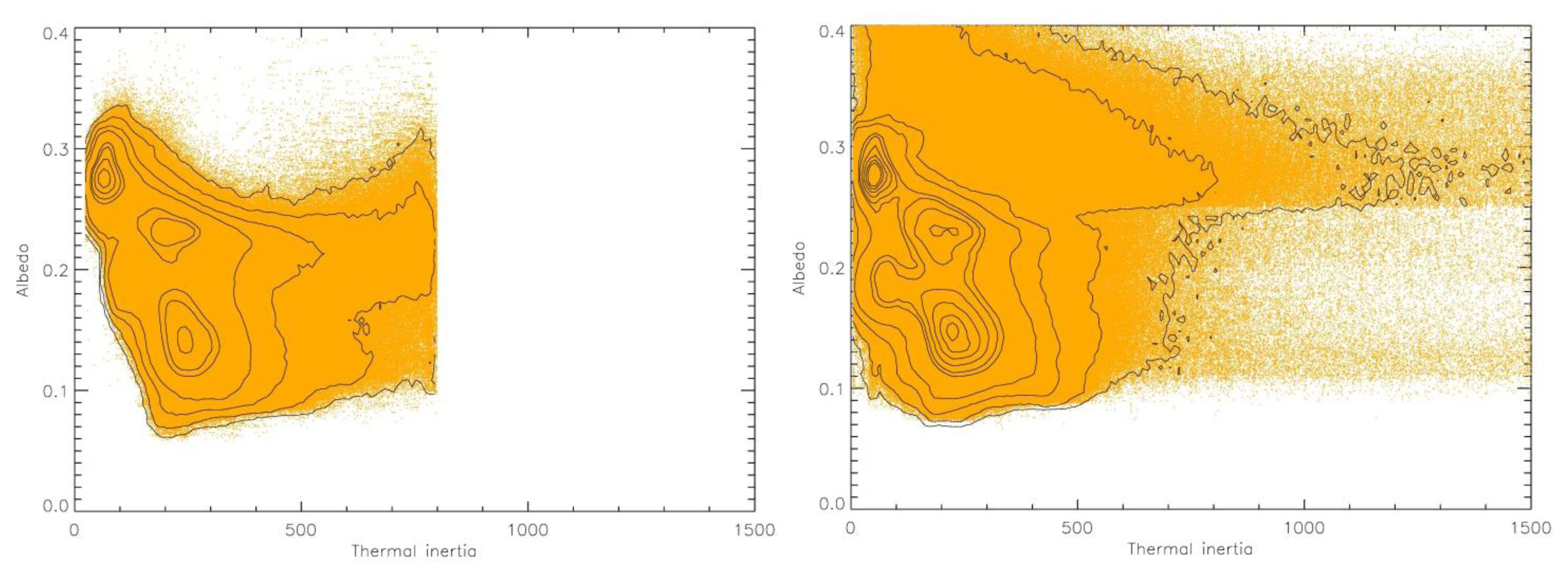This thermal inertia dataset differs from that utilized by previous works [7,8] (Figure 2), as the earlier model for deriving thermal inertia only computed values within the range of 0–800 tiu [8]. Thermal inertia values > 800 tiu encompass 5.7% of the newer 2007 map, so only a small fraction of pixels have values outside the earlier (2005–2006) model, but these thermal inertia values indicate distinctive surface characteristics (Table 1). Additionally, the greater geographic coverage of the 2007 thermal inertia map introduces values that may differ from the interpolated values in the earlier maps. Additionally, the thermal inertia dataset used here is more complete than that used in the thermophysical mapping of [8] where observations constituted 60% [57].

3. Methods

The three algorithmic classification methods used in this study—Expectation Maximisation (EM) of a Gaussian Mixture Model (GMM), ISODATA, and ISODATA combined with MAXLIKE—are described below. These algorithms were chosen as they are frequently used for clustering of multivariate datasets but each differs in their determination of classes and/or their measure of pixel similarity. Each algorithmic classifier has been shown to be capable of providing efficient and accurate partitioning of multivariate datasets (e.g., EM with GMM: [102–106]; ISODATA [107–109]; ISODATA + MAXLIKE [110–113]). EM is typically used to estimate the parameters of an underlying distribution, and to provide a parametric measure of clustering [104,114–117]. ISODATA is applied to autonomously determine class boundaries and assign pixels to classes by applying a minimum distance measure for pixel similarity. The Maximum Likelihood Classifier (MAXLIKE) is a supervised clustering algorithm that obtains class parameters from either training data, or the output of another unsupervised classifier such as ISODATA. In the latter case, MAXLIKE reassigns pixels based on the ISODATA output by applying a probabilistic measure of similarity. The combination of ISODATA and MAXLIKE has been widely used in environmental remote sensing using multispectral imagery [67,118] and has made valuable contributions to the unsupervised mapping of Earth land cover by providing accurate information when operated on two or more independent datasets [119–121]. All three of these algorithms are either inbuilt into common software packages for remote sensing and GIS (e.g., ENVI, ArcGIS, ERDAS Imagine, IDRISI, etc.), or are freely available as code for implementation into common analysis software packages (e.g., IDL, Matlab, etc.). In this work, each of these algorithms will be used to delineate seven two-dimensional classes in thermal inertia and albedo, to compare with recent previous 7 class thermophysical maps [8,9].

3.1. Expectation Maximisation for a Gaussian Mixture Model

To indirectly identify the number of natural classes within a two dimensional dataset, one approach is to determine the intrinsic structure of the data by fitting the density of observations [122]. This can be achieved by applying a mixture model in which the observations are assumed to originate from a linear combination of multiple unknown probability distributions. Each grouping within the data is then described by a single probability density function (pdf), with the parameters of that pdf describing the centre and spread of the class [123]. Determining density functions can be a difficult challenge, but the problem can be simplified by the assumption that the data points within each class originated from a Gaussian distribution, with N Gaussians required to describe the whole space. The aim is then to determine the number of Gaussians and the parameters of those Gaussians which best replicate the dataspace. The assumption of Gaussian clusters is justified in this work as both albedo and thermal inertia datasets have primary modes shaped like Gaussians (Figure 1), and hence can likely be approximated by the sum of a finite number of Gaussian distributions. This approach of a Gaussian Mixture Model (GMM) is referred to as a generative model, as first a model is developed which is able to generate the dataset, and subsequently the model is applied to the classification of points.

To determine the set of parameters for N Gaussians which will result in the highest probability (maximum likelihood) of generating the dataset, the Expectation Maximisation (EM) algorithm is used. EM operates by optimising a given criterion (the likelihood function in this case), by iteratively calculating the expected value of the function (expectation step) and using the response to estimate the input parameters (maximisation step) [124,125]. The Expectation Maximisation (EM) algorithm is then applied to describe the underlying Gaussians—their mean, standard deviation/variance, and amplitude—by maximising the likelihood of a set of Gaussian parameters generating the observed data. The GMM provides a fit F(x,y) to the density of the dataspace through:

$$F(x,y)=n=1n={\text{N}A}_{n}G(x,y;{\overline{x}}_n;{\overline{y}}_n;{\mathrm{\sigma }}_{xn};{\mathrm{\sigma }}_{yn})$$

(1)

where N indicates the number of Gaussians in the mixture model, A_n are the Gaussian amplitudes, σ_xn and σ_yn are the standard deviations and χ̄_n and ȳ_n are the means. The frequency of a given x, y value occurring within the dataspace modelled by the bivariate normal distributions is given by [126]:

$$G(x,y\mid n=\text{N})=\frac{e^{-Q_n/2}}{2\mathrm{\pi }{\mathrm{\sigma }}_{xn}{\mathrm{\sigma }}_{yn}\sqrt{1-{p_n}^2}}$$

(2)

where

$$\begin{array}{c}{Q}_n=\frac{1}{1-{p_n}^2}\times \left[{\left(\frac{x-\overline{x_n}}{{\mathrm{\sigma }}_{xn}}\right)}^2+{\left(\frac{y-\overline{y_n}}{{\mathrm{\sigma }}_{yn}}\right)}^2-\frac{2p_n(x-\overline{x_n})(y-\overline{y_n})}{{\mathrm{\sigma }}_{xn}{\mathrm{\sigma }}_{yn}}\right]\\ p_n=\frac{cov(x,y)}{{\mathrm{\sigma }}_{xn}{\mathrm{\sigma }}_{yn}}\end{array}$$

The EM algorithm iteratively calculates the expected value of the log likelihood function, and then maximizes this function with respect to the parameters of the N probability density functions. The log likelihood is used as it is analytically easier to maximize than the likelihood function [125]:

$$L({\mathrm{\theta }}_n)=\sum _{t=1}^{K}logP(x_t,y_t\mid {\mathrm{\theta }}_n)$$

(3)

where the x_t, y_t are from a set of K independent, identically distributed samples [127], θn is the set of parameters A_n, σ_xn, σ_yn, $\overline{x_n}$ and $\overline{y_n}$ for each density function; and P is the probability of each data vector from the weighted sum of the N Gaussian distributions (the normalised form of Equation (1)).

The EM algorithm applied here was the publicly available procedure ex_max.pro [128] from the Princeton University IDL Utilities library.

Initialisation

The main difficulty of using the EM algorithm lies in choosing appropriate initialisation parameters. The algorithm can become easily trapped within local minima/maxima of the likelihood function [60,129]. The algorithm will automatically exit when the covariance matrix becomes close to singular (unable to be inverted). This can occur due to collinearity within a class (high covariance), a small number of points within a class, or if the number of Gaussians at initialisation is larger than the number of natural groupings within the data.

Various initialisation parameters were tried for Gaussian Mixture Models using from 3–7 Gaussians (Figure 3). The results for seven Gaussians (Figure 4) are used for analysis for direct comparison with the most recent thermophysical classifications of [8,9]. For n > 5 the algorithm did not successfully converge unless outliers were removed. Outliers were defined as values above 0.4 in albedo or above 1500 in thermal inertia, comprising ~0.01% of the data. This reflects the sensitivity of the algorithm to the initial parameters and the inclusion of outliers. The EM algorithm was found to be insensitive to the choice of initial amplitude (A_n) and initial mean vectors ( $\overline{x_n},\overline{y_n}$), but very sensitive to the choice of initial variances (σ_xn²; σ_yn²). For the seven Gaussian model the initialisation parameters were:

• Mean albedo, thermal inertia values of (0.15, 500), (0.27, 10), (0.23, 500), (0.15, 10), (0.15, 1000), (0.08, 100) and (0.30, 100);
• Albedo and thermal inertia variances of 0.05 for each Gaussian;
• Amplitude of 10³ for each Gaussian.

To decrease processing time, the EM algorithm was run on every 10th data point (2592,000 in total- corresponding to a separation of 0.05 degrees in latitude and 0.1 degrees in longitude), taking approximately 8 h to complete each run on an i5 processor. The output of the algorithm for seven Gaussians is given in

Table 3. Best fit parameters from Gaussian Mixture Model with seven Gaussians.

Parameters	Gaussians
	1	2	3	4	5	6	7
Albedo mean	0.288	0.231	0.138	0.243	0.275	0.167	0.276
Inertia mean	63.0	209.4	237.3	89.1	50.6	217.9	456.8
Albedo var.	0.0002	0.0004	0.0003	0.0031	0.0001	0.0006	0.0039
Inertia var.	529.8	4221.7	1667.8	937.7	237.8	8193.7	6,9217.9
Covariance	−0.121	−0.550	0.018	0.613	−0.009	−1.353	−2.531
Amplitude	156,401.8	644,017.5	403,102.0	129,761.3	128,220.0	878,449.9	98,743.5

, in the form of the Gaussian parameters which provided the maximum likelihood fit to the actual counts (the density) of the albedo-thermal inertia dataset. The algorithm exits when the centroids of each Gaussian and the assignment of data points to each Gaussian do not change between iterations [61].

The output of the GMM is a prediction F(x,y) of the expected number of counts for each value of albedo and thermal inertia, which are shown in Figure 5. The GMM fit failed consistently in that the total amplitude of F(x,y) at the centres of the three dominant modes was a factor of ~2 larger than the histogram for the observed data (Figure 5). This is most likely due to a breakdown in the assumption of a Gaussian data distribution outside of the local modal peaks. A Gaussian distribution appears appropriate for fitting values near the four modal peaks (Figure 1), but is likely less appropriate for fitting low frequency data values further from the modal peaks, such as those with medium-high thermal inertia. The broad (large standard deviation) Gaussians that EM assigns to fit these data values leads to significant overlap with the Gaussians fitting the modal values, and hence an overestimate in pixel counts. For this work however, the focus is on defining classes rather than density estimation, so to assign pixels to classes, the counts from each Gaussian were summed and normalised. In other words, for each value of thermal inertia and albedo, the prediction from each of the N Gaussians was divided by the total fit (F), thereby providing an estimate of the probability P(x,y) that the observed datapoint x,y came from the nth distribution. Pixels were then assigned to the class which had the highest probability. The second highest probability class for each pixel was also examined. The assignment of pixels is analysed in Results.

3.2. ISODATA

ISODATA is an unsupervised clustering algorithm that aims to approximate the natural structure of a multidimensional dataset by iteratively passing through the data and defining classes by minimizing the pixel separation values (Equation (4)) [130] and therefore minimising the sum of squared error (SSE; Equation (5)). The ISODATA algorithm is particularly powerful when little is known about the data prior to classification as it makes no assumptions on the underlying probability distribution of the datasets [108,131,132]. The user inputs the maximum number of classes to identify (N), allowing the algorithm to choose N equally separated initial seeds that span the dataspace along the line connecting the min and max data values [133]. The position of the initial seeds is not crucial to the final clustering, provided that the algorithm is given enough processing time [134]. ISODATA adjusts the number of classes iteratively and can merge and split classes that have similar values [109,130], and will output less than or equal to N classes. Additional input parameters are the convergence threshold—the minimum number of pixels which must be unchanging between iterations before the algorithm can cease—and the maximum number of iterations which the algorithm can execute [130,131,135].

The N initial seeds represent the centres of N initial classes. A pixel is assigned to a class if its separation distance from the centre of the class is less than its distance to all other class centres. ISODATA partitions pixels into classes by progressively minimising the pixel separation and the SSE. In two dimensions, the pixel separation from a class centre is given by [135]:

$$D=\sqrt{{(x-\overline{x})}^2+{(y-\overline{y})}^2}$$

(4)

where D = separation distance; (x,y) = pixel vector; and (χ̄, ȳ) = cluster mean vector. Once all pixels are assigned, each class centre is recalculated by taking the mean of pixels assigned to the class [136]. The process then continues iteratively. The assignment of pixels is independent of the contiguity of the pixels in the spatial frame and hence pixels within the same class can have a large spatial separation on the classified map. The sum of squared error for each cluster is given by:

$$SSE=\sum _{i=1}^n{(x-\overline{x})}^2$$

(5)

where n = the number of pixels/datapoints within the cluster. Hence minimising pixel separation also minimises the SSE within each class.

Input Parameters

The ISODATA algorithm was run for a maximum number of 4–14 classes (Figure 6). The output of seven classes is presented in Figure 7 and analysed in this work. The input parameters producing seven classes were:

• 99% convergence threshold;
• Maximum of 500 iterations;
• Maximum number of seven classes;
• Albedo and thermal inertia dataset. Algorithm was run both with outliers excluded, and with outliers included. Outliers were defined as values above 0.4 in albedo or above 1500 in thermal inertia, comprising ~0.01% of the data.

The albedo and thermal inertia datasets were both normalized prior to classification by linear transformation to the range [0, 1]. As albedo and thermal inertia have different physical meanings and different ranges of values across the Martian surface, this normalization allowed them to contribute equally in the calculations of pixel separation [135]. The importance of this step is illustrated in Figure 8 and

Table 4. Testing the robustness of ISODATA to scaling of input variables.

Map Description	Scaling of Albedo and Thermal Inertia				Resulting ISODATA Classification Sensitive to Data Histogram
	Variables on Same Range	Variables Normalised	Linear Transformation Applied	Variable on Larger Range
No scaling Albedo [0, 0.6], Thermal Inertia [0, 5000]	NO	NO	YES	Thermal inertia	No *
Albedo unchanged, log of thermal inertia A [0, 0.6], TI [small, 3.7]	NO	NO	NO	Thermal inertia	No
Albedo and thermal inertia normalised to range [0, 1]	YES	YES	YES	n/a	Yes
Albedo and thermal inertia scaled to range [0, 15]	YES	NO	YES	n/a	Yes
Albedo scaled to range [0, 10], thermal inertia normalised to range [0, 1]	NO	NO	YES	Albedo	Yes
Albedo and thermal inertia normalised and then squared [0, 1]	YES	YES	NO	n/a	Yes

^*The lack of sensitivity to the underlying data distribution is illustrated in Figure 8.

. The partitioning of pixels into classes (observed through a scatterplot), and hence the resulting spatial pattern in the classified map, was robust to the type of scaling applied to albedo and thermal inertia (linear or non-linear, Table 3) provided that both variables had the same range. A fine partitioning of thermal inertia into classes (with little sensitivity to the albedo dataset) was observed when the input datasets were not scaled, indicating that the algorithm was much more sensitive to the larger-scale structure in thermal inertia than it was to the finer-scale structure in albedo (Figure 8). Removing the outlying values was found to improve the performance of the ISODATA algorithm, consistent with the findings of other works assessing the analogous k-means algorithm [137,138], however the combination of the ISODATA algorithm with Maximum Likelihood was robust to the inclusion of outliers, in that it produced similar class statistics to that of ISODATA and Maximum Likelihood including outliers. Even with the removal of outliers, several classes were bimodal in one or both parameters (Figure 7). This may be improved by a broader inclusion of outlying values, which would come at the cost of excluding meaningful surface environments from the classification. Alternatively, bimodality may be removed by allowing the algorithm to output a higher number of classes and more finely partition the data.

The algorithm was not sensitive to the maximum number of iterations as <50 iterations were required to meet the convergence threshold for all values of N, and thus the convergence threshold of 99% determined the algorithm exit.

3.3. Maximum Likelihood

A maximum likelihood classifier (MAXLIKE) was used for supervised classification as it is commonly paired with ISODATA to deal with pixels near the boundary of a training class [107,135]. The statistics describing each of the classes provided by ISODATA (mean and covariance) provide input for MAXLIKE [130], which assumes that the distribution of each class will be multivariate normal depending on the number of parameters in the classification. The probability of a pixel belonging to a given class is provided in our case by the bivariate normal distribution probability density function (Equation (2))—analogously to the Gaussian Mixture Model—with each pixel assigned to the class to which it has the highest probability of being a member.

It is this probabilistic logic which provides a different partitioning of the dataset to that provided by ISODATA at the boundary regions between ISODATA classes. The majority of pixels are assigned to the same class by MAXLIKE as they were by ISODATA, because pixels near a given class centre have a high probability of being assigned to that class. The classification of pixels into seven classes is shown in Results. Near the boundary between classes it is not clear from ISODATA which class is most similar to a pixel as it may be equidistant from two class centres. By calculating Gaussian membership probabilities, MAXLIKE provides a statistical methodology for assigning pixels to classes when they are equidistant from two class means [139,140].

The MAXLIKE algorithm is most effective with a normal distribution of data [141]. If the histograms of the input parameters are strongly non-normal the algorithm can overestimate χ² (chi-squared) classification errors [142]. This problem is minimized with an increasing number of data points in the total sample and has been found to be negligible if the number of data points is >400 [142,143] and hence should have a minimal effect on the classification here (>10⁷ pixels).

3.4. Classification Confidence

The accuracy of algorithmic clustering and classification would typically be determined using groundtruthing data to identify the percentage of correctly classified pixels [144]. Studies that have assessed the overall accuracy of an unsupervised classification such as ISODATA paired with the maximum likelihood classifier reported accuracies of 60%–90% [110–113]. Gaussian Mixture Models developed by EM algorithms have reported accuracies of 90% [145–147]. Hence the techniques applied in this work are demonstrably capable of providing classifications that translate into useful and accurate information on surface materials.

With regard to Mars the option of extensive field sampling is unavailable. To validate cluster we are therefore limited to a statistical discussion of the pixel assignment accuracy, and groundtruthing through comparison to independent orbital datasets and limited sampling locations on the surface (see Discussion). The algorithms applied in this work classify all pixels, irrespective of how small the probabilities of class membership are. Poor classification can result for pixels lying near the tails of the distribution function for each class, where they may be equidistant from more than one class centre or may have equal membership probabilities from more than one Gaussian distribution. Figures 9 and 10 provide the relative classification confidence based on the separation distances between each pixel and the mean of its assigned class (calculated from Equation (4)). Pixels with small separation from the class mean are more likely to be correctly classified than those nearer the class decision boundary. Both EM of a GMM and the ISODATA + MAXLIKE classifiers performs their best at the mid- to low-latitudes, and both show lower classification confidence in the polar regions. The regions of low confidence identified by each of the algorithmic classification methods indicate where the interpretation of pixels should be undertaken with caution.

4. Results

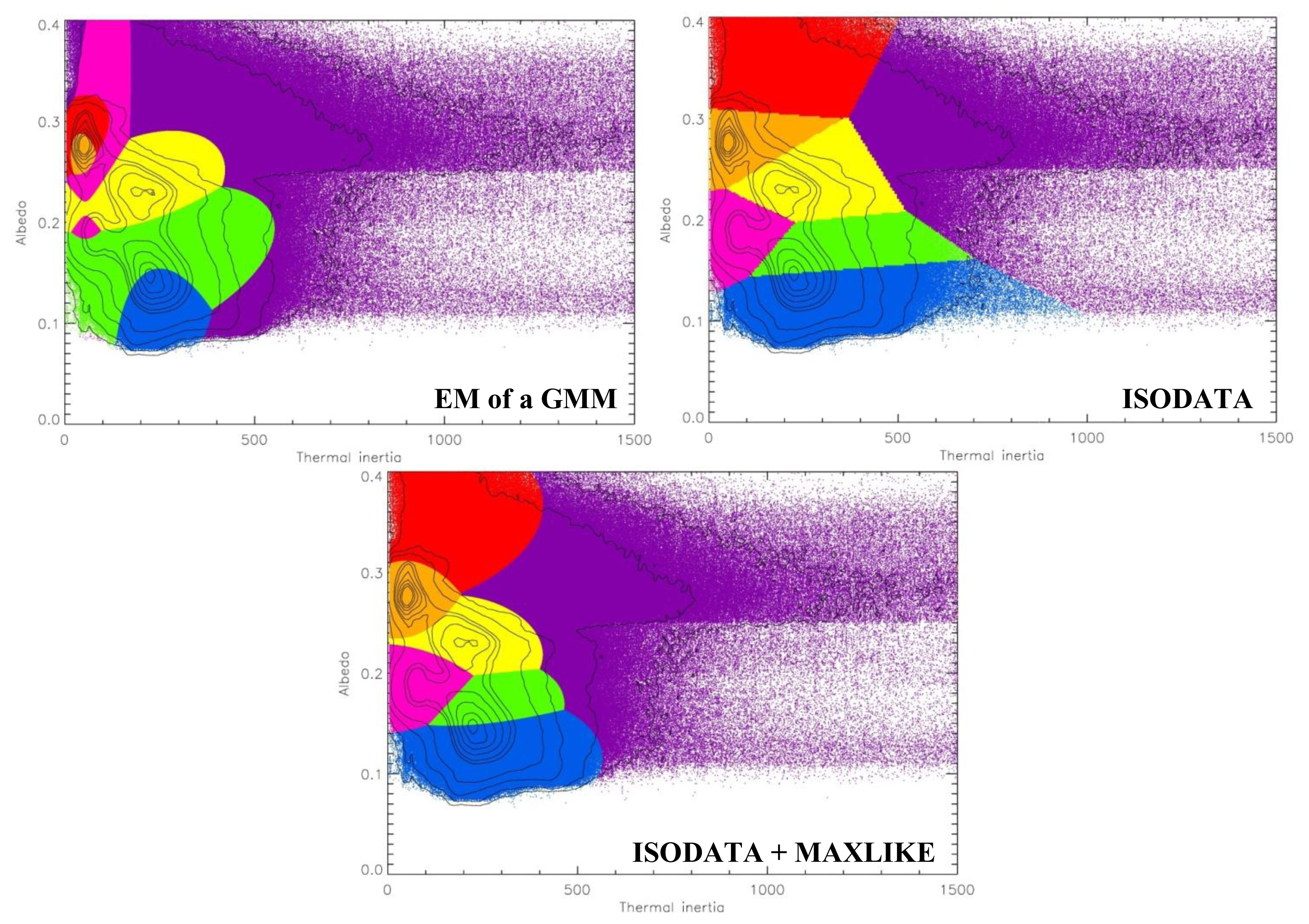
The results of each classifier are shown as a scatterplot in Figure 11 and summarised in

Table 5. Details of the seven classes produced by each method.

Class	Parameters	Gaussian Mixture	ISODATA	ISODATA + MAXLIKE
Yellow (class 4)	Albedo mean	0.23	0.23	0.23
	Inertia mean	194	219	214
	Albedo sd.	0.018	0.015	0.015
	Inertia sd.	64	63	58
Red (class 7)	Albedo mean	0.29	0.34	0.34
	Inertia mean	62	153	153
	Albedo sd.	0.011	0.027	0.029
	Inertia sd.	23	111	96
Green (class 2)	Albedo mean	0.17	0.17	0.17
	Inertia mean	226	250	244
	Albedo sd.	0.018	0.013	0.013
	Inertia sd.	87	59	53
Fuchsia (class 3)	Albedo mean	0.125	0.19	0.19
	Inertia mean	90	115	115
	Albedo sd.	0.048	0.015	0.015
	Inertia sd.	31	49	49
Blue (class 1)	Albedo mean	0.13	0.13	0.13
	Inertia mean	253	264	263
	Albedo sd.	0.014	0.013	0.014
	Inertia sd.	41	70	66
Orange (class 6)	Albedo mean	0.27	0.28	0.28
	Inertia mean	51	74	70
	Albedo sd.	0.008	0.016	0.016
	Inertia sd.	13	39	32
Purple (class 5)	Albedo mean	0.27	0.28	0.27
	Inertia mean	531	684	588
	Albedo sd.	0.085	0.046	0.054
	Inertia sd.	255	247	240

. The algorithmic classification methods applied in this work do not involve deterministic bias, yet it is essential to examine whether the results provide a reasonable partitioning of the dataspace. This is particularly important as in all methods the maximum number of classes was chosen prior to classification. An optimal classification has class boundaries closely aligning with features in the underlying distribution of values, so that the maximum amount of information is extracted from thermal inertia and albedo without the introduction of false patterns due to over-partitioning [129,148].

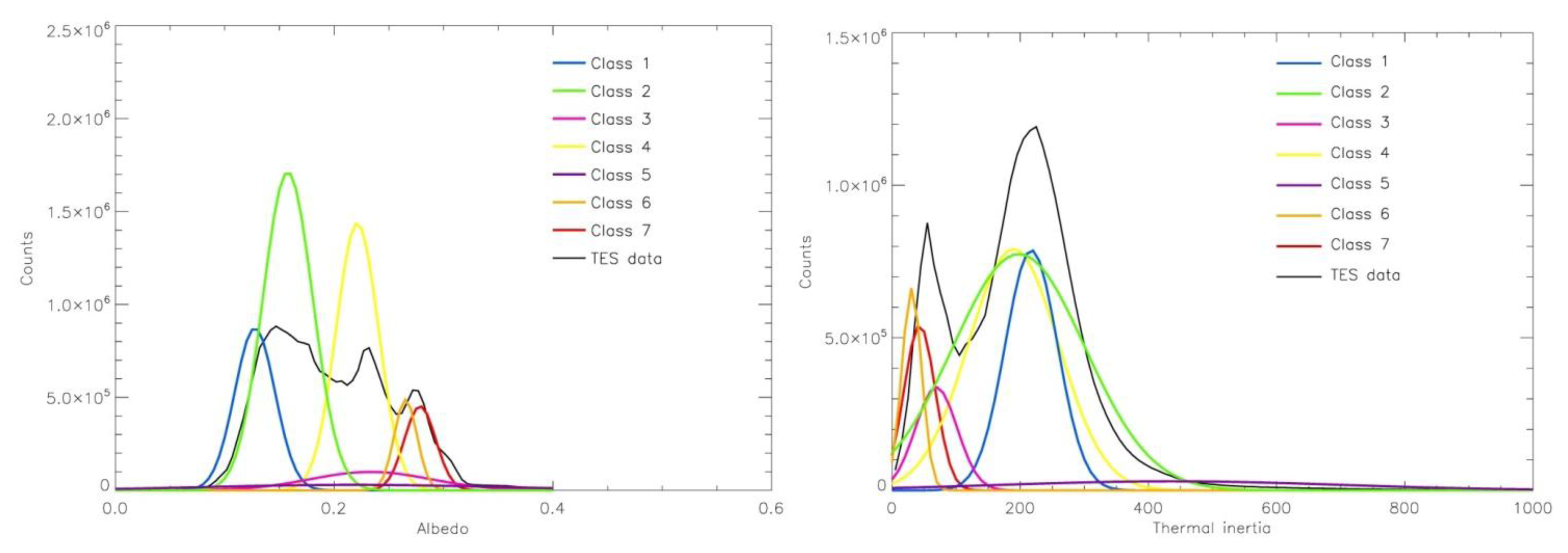
Comparing Figure 3 with Figure 6 reveals that the GMM results with five classes show the best alignment between class boundaries and the modal peaks in the data histogram—indicating that this classification scheme can perform very well for small numbers of classes. For seven classes, two modal peaks align with Gaussians (orange and yellow in Figure 11). These Gaussians also align with peaks in the global thermal inertia and albedo histograms (Figure 5). Other class boundaries from the seven Gaussian classification do not align well with the data structure. For example, class 5 (purple) appears to be assigned to reproduce the pixel counts in moderate to high thermal inertia, however some pixels at low thermal inertia and high albedo are assigned to the class when they would appear to more naturally fit within class 3 (fuchsia). In addition, the GMM algorithm did not converge for more than five classes when outliers were included within the dataset, indicating that it can be strongly skewed by data values even if the counts are very low. Finally, from Figure 5, the EM of a GMM algorithm does a poor job of reproducing the total counts within the dataset, overestimating them by a factor of >2. This last point is also true even for the five Gaussian classification.

The ISODATA plus Maximum Likelihood classification also shows good alignment with the data structure for five classes (Figure 6), although some class boundaries (e.g., the green class) are not aligned as well as they were in the GMM with five Gaussians. Unlike in the EM of a GMM classification, however, the alignment of classes with the data structure improves as the number of classes increases. For both the combined ISODATA + MAXLIKE and ISODATA on its own with seven classes, three of four modal peaks are aligned with a distinct class. The fourth modal peak is divided between the green and blue classes. This division appears somewhat arbitrary based on the data structure, however in the Discussion we will show that some coherent subdivisions like this can provide geologically useful information. The classes produced by the combined ISODATA + MAXLIKE algorithms are generally bimodal in thermal inertia and/or albedo (Figure 7). This could suggest that a larger number of coherent classes can be identified, for example class 4 (yellow) incorporates a broad range of albedo values that may be better subdivided to remove the class bimodality. Alternatively, bimodality may reflect poor placement of the class boundary. In summary, for seven classes, the ISODATA assignment combined with the refinement undertaken by MAXLIKE shows greater sensitivity to the underlying data structure than the GMM (Figure 11).

An additional measure of improved clustering is a decrease in the intra-cluster variance, which is analogous to increasing the similarity among the pixels assigned to the class [149,150]. From Table 5 the classes produced by ISODATA and MAXLIKE generally show lower variance for either one or both parameters than those produced by EM of a GMM, suggesting that clustering could be improved by subdividing some of the GMM classes [151]. Two GMM classes (red and orange) have lower variances in both albedo and thermal inertia. It is difficult to compare the variance of the GMM classes to those of the other classifiers however, given the significantly different placement of class boundaries by the GMM algorithm (Figure 11). The Maximum Likelihood method is at least as good as ISODATA on its own for the yellow, green, fuchsia, and orange classes in Table 5. One artifact of the ISODATA algorithm is the straight line delineation between classes due to the Euclidean distance measure used by the algorithm to partition the data [119,152]. These boundaries cut across contours and are not a natural division within the data. The Gaussian decision criteria applied by MAXLIKE and EM of a GMM produces elliptical classes [153], which appear to perform better at aligning the class boundaries with the underlying pixel density.

In summary, the combination of ISODATA and MAXLIKE identifies the largest number of coherent classes which are aligned with the data structure. In addition, the intra-cluster variances from this combination are at least as good as those from ISODATA alone for seven classes. Thus the Maximum Likelihood classifier provides an improvement in sensitivity for delineating class boundaries over ISODATA on its own, and EM of a GMM. The discussion of the resulting spatial map and interpretation of the classes will therefore focus on the classification produced by the combination of ISODATA and MAXLIKE.

5. Discussion

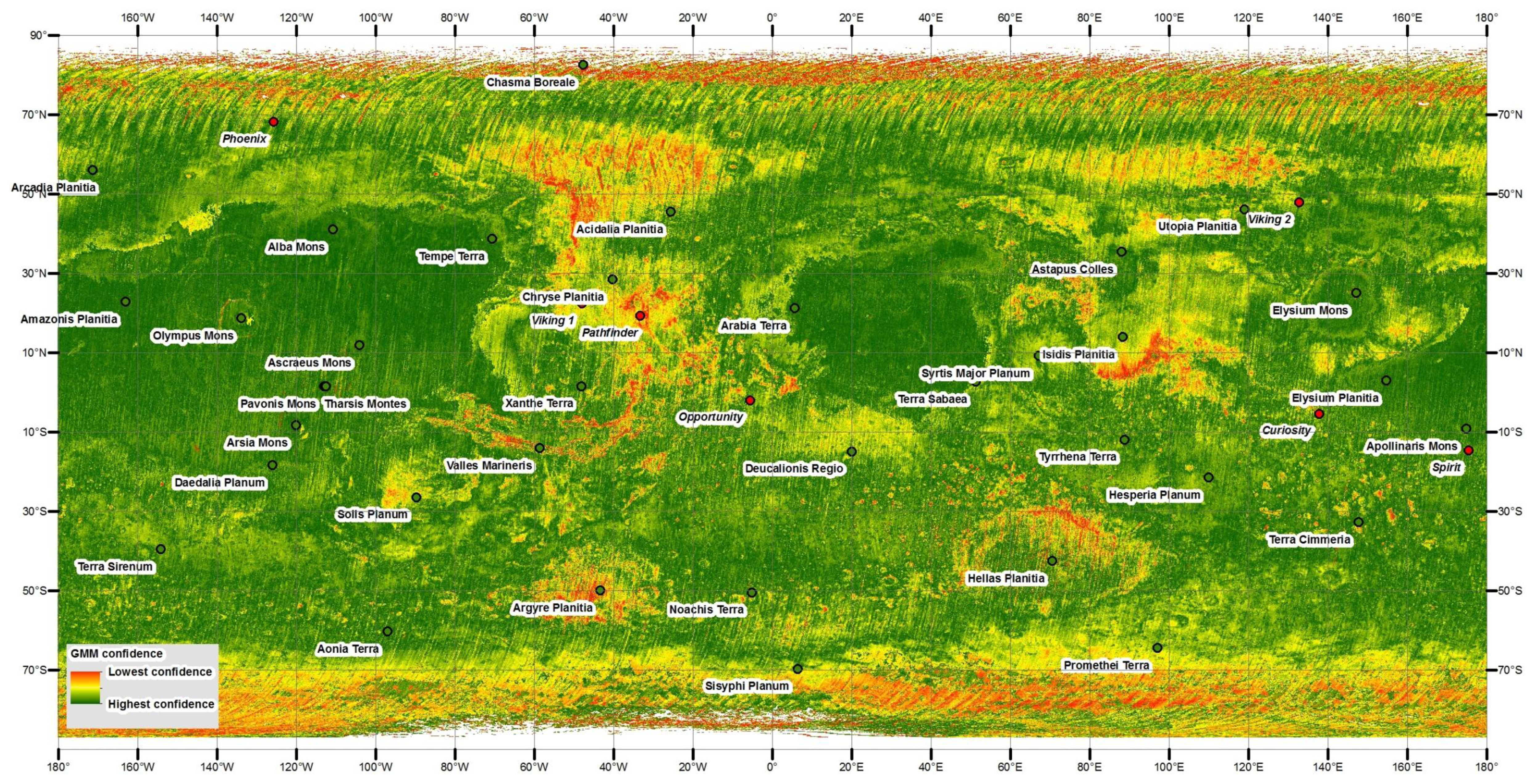
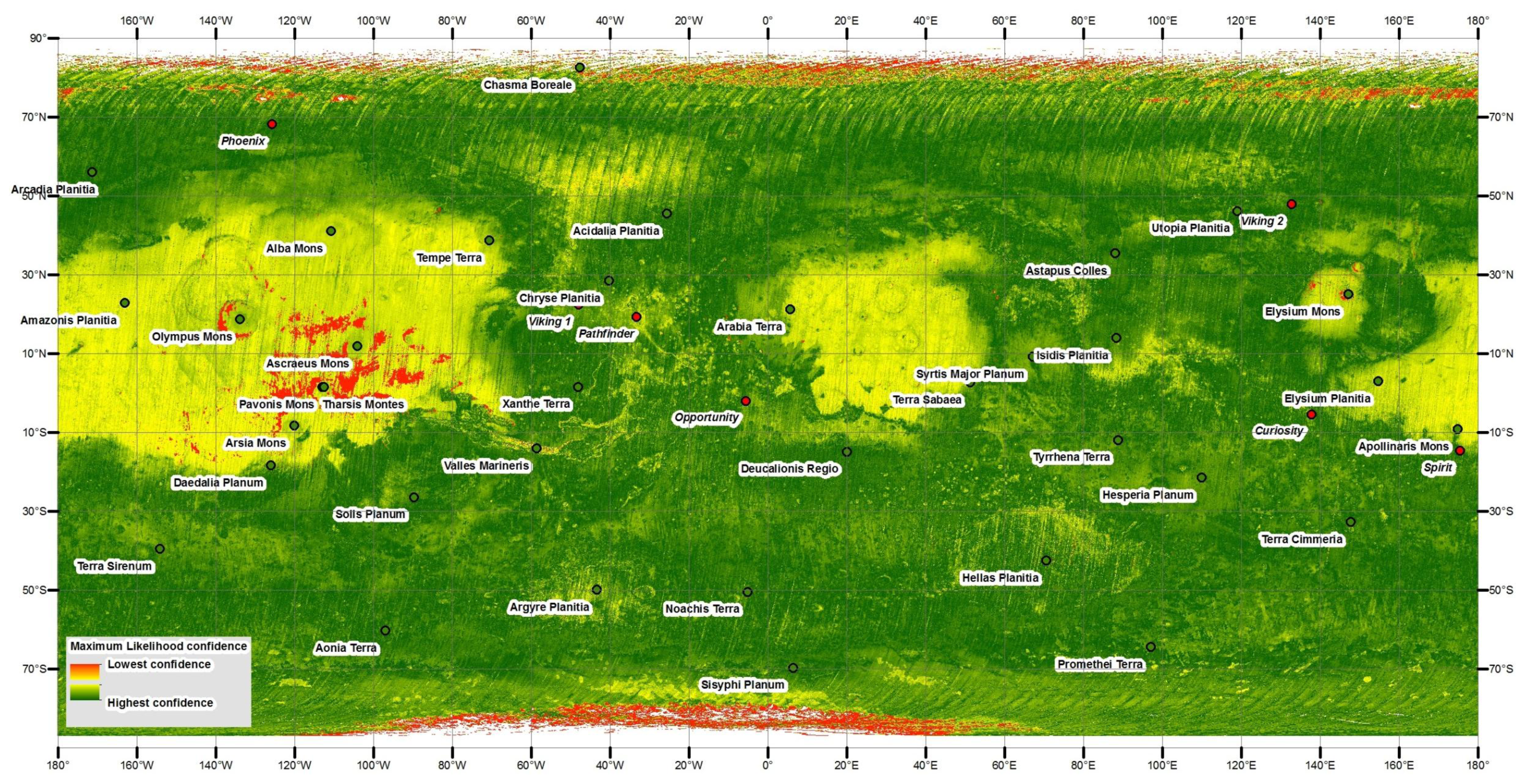
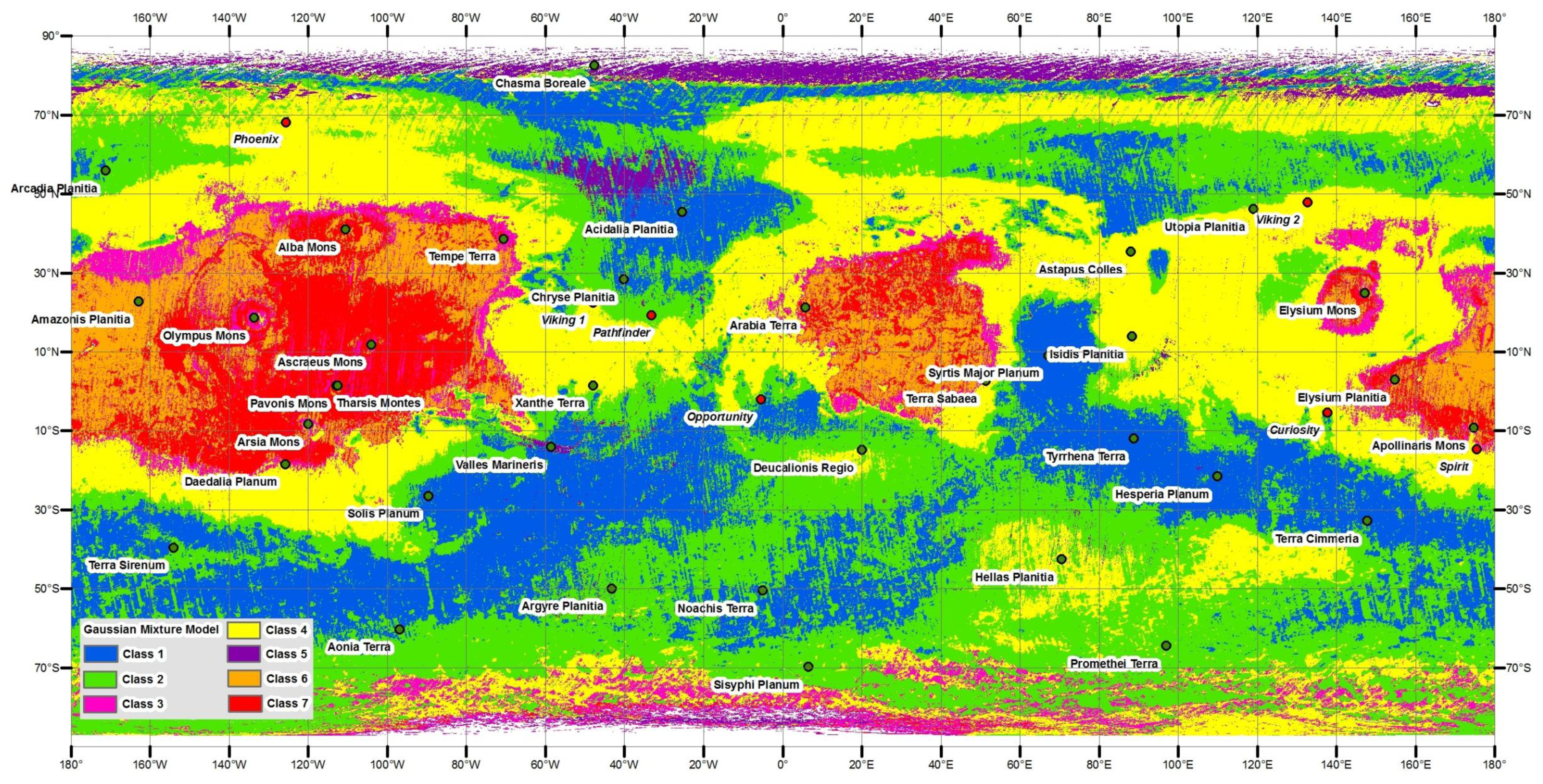
The classification maps in Figures 12 and 13 show a strong coherent spatial pattern of concentric class occurrence in both hemispheres, moving from the equator to higher latitudes. No spatial information was involved in the classification. This concentric class sequence corresponds to a general decrease in albedo moving outwards from the equator through the classes, accompanied by a general increase in thermal inertia. The trend is broadly due to decreasing surface dust coverage [15] and fine grained sand as well as an increasing exposure of coarse grains, rocks [14] and duricrust with distance from the equator [21]. The classification of thermal inertia and albedo into fine dust-sized grains being dominant in the low latitudes, coarse sand in the mid-latitudes, and ice at the high latitudes, is consistent with previous thermophysical maps [7,8]. Generally, the global spatial patterns in surface materials are robust to the choice of classifiers applied in this work and consistent with previous works. From the pixel distance maps in Figures 9 and 10, both the EM of a GMM and ISODATA + MAXLIKE classification have lower classification confidence in the polar regions. This is likely due to the spatial incoherence in the thermal inertia dataset, derived from the large variations in thermal inertia between the seasonal maps in this area [10]. The moderate classification confidence at low latitudes appears to correspond to the placement of the orange-yellow-fuchsia class boundaries in Figure 11. In general, the classification confidence in Figure 9 shows an inverse relationship with thermal inertia—with lowest classification confidence occurring in regions of high thermal inertia (Figure A1). The high classification confidence regions of Figure 10 correspond to areas of low thermal inertia and high albedo (Figures A1 and A2).

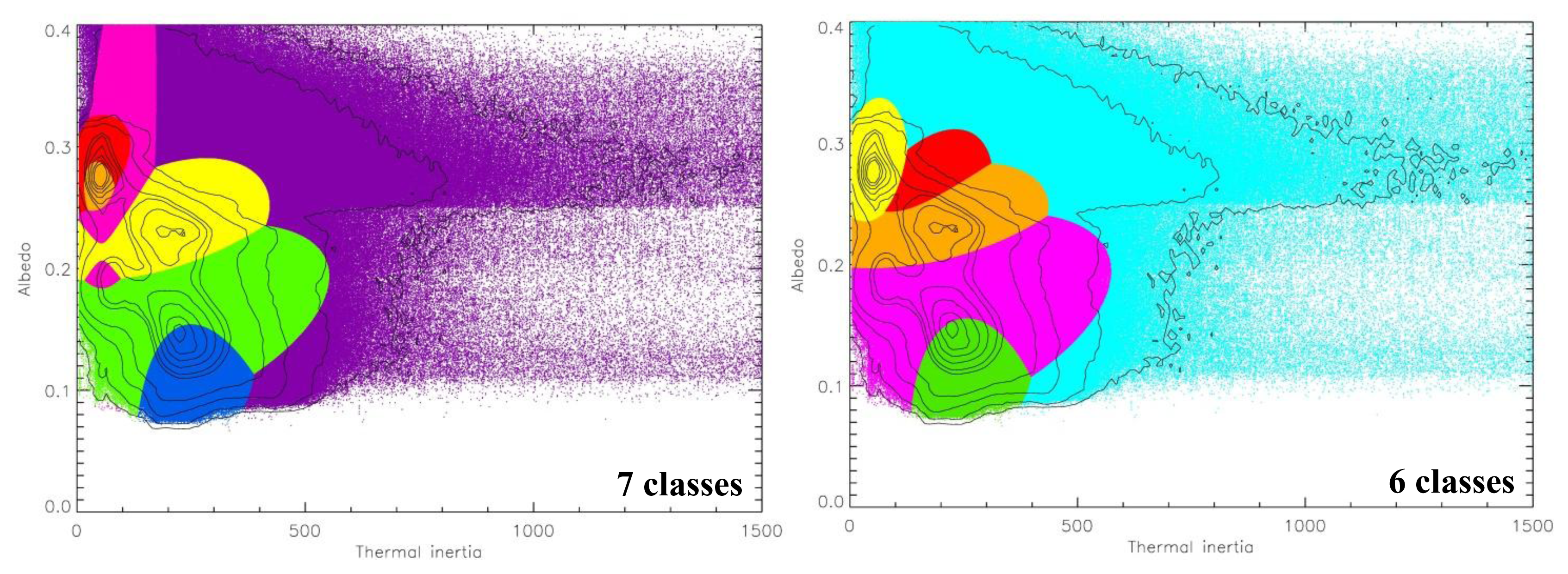
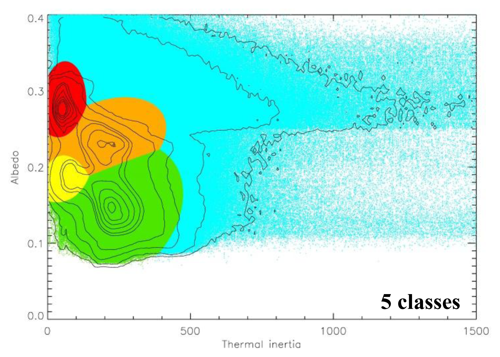
It is difficult to directly compare this work with previous thermophysical classifications due to the differences in the thermal inertia and albedo datasets (Figure 2). Figure 14 compares the manual classification of [8] to the output of the automated classification algorithms used in this work, applied to the same older datasets. In the manual classification, the three major modal peaks are each encompassed within a class (blue, yellow and red), however there are divisions for the rest of the data which do not appear aligned with the underlying data structure. Furthermore, several of the classes encompass a broad range of thermal inertia and albedo values which corresponds to a broad range of surface materials. For example, the fuchsia class encompasses materials with thermal inertia values ranging from 50–400 tiu, corresponding to particles sizes ranging approximately from 5 μm to 2 cm [16,18] (Table 1) and possibly therefore environments with varied erosional histories. From Figure 14, the 5 class classification produced by ISODATA and Maximum Likelihood on the older data set is the only one which does not place a boundary cutting across one of the local maxima. The 7 class automated classification—using the same number of partitions as [8]—places several of the class boundaries in significantly different locations to the manual classification, and subdivides two of the modal peaks (blue and green; yellow and red). These subdivisions appear artificial from the viewpoint of the global data structure, however some subdivisions may be useful for geological mapping as discussed below.

The most recent mapping of thermophysical units using the same thermal inertia dataset as in this work was done by [9,57]. The most significant difference between the class boundaries in that work and previous mapping by [8] occur in the boundary between units F and G, which is placed by [9] around albedo ~0.24, and thermal inertia > 403 tiu. The analogous classes in the mapping of this study are classes 5 (purple) and 7 (red) (

Table 6. Interpretation of thermophysical units.

Units from [8,9,57]	Most Similar Classes from this Study	General Interpretation of Dominant Surface Materials in Classes from this Study
A	Orange (class 6)	Thick covering of dust and bright unconsolidated fines, some exposures of darker fine sand. Generally grains < 100 μm.
B	Green (class 2)	Fine-coarse sand, some duricrust, and low dust coverage. Grainsize generally > 60 μm and < 3 mm.
C	Yellow (class 4)	Mixture of bright dust and fine sand, with a small fraction of coarse sand and duricrust. Grains predominately < 1 mm.
D	Fuchsia (class 3)	Fine sand with some dust covering. Similar to orange (class 6) but with a lower subpixel coverage of bright fines. Grains <100 μm.
E	Blue (class 1)	Dark fines, with some coarse sand and duricrust; very little dust. Grains < 3 mm.
F	Purple (class 5)	Dominated by pebbles, boulders, ice-cemented soil, and exposed ice. Some duricrust and sand. Dust coverage varies. Grains > 100 μm.
G	Red (class 7)	Bright dust covering fines, duricrust, and ice-cemented soil. Some exposed ice but with a substantial fine component.

). The boundary between these class occurs around a similar thermal inertia range of >400 tiu, but a higher albedo of ~0.3 (Figure 11), and cuts across the 5.5 × 10⁴ count contour in Figure 11. The boundary between the class F-G boundary in [9] is more sensitive to the drop in counts observed at low albedo and high thermal inertia.

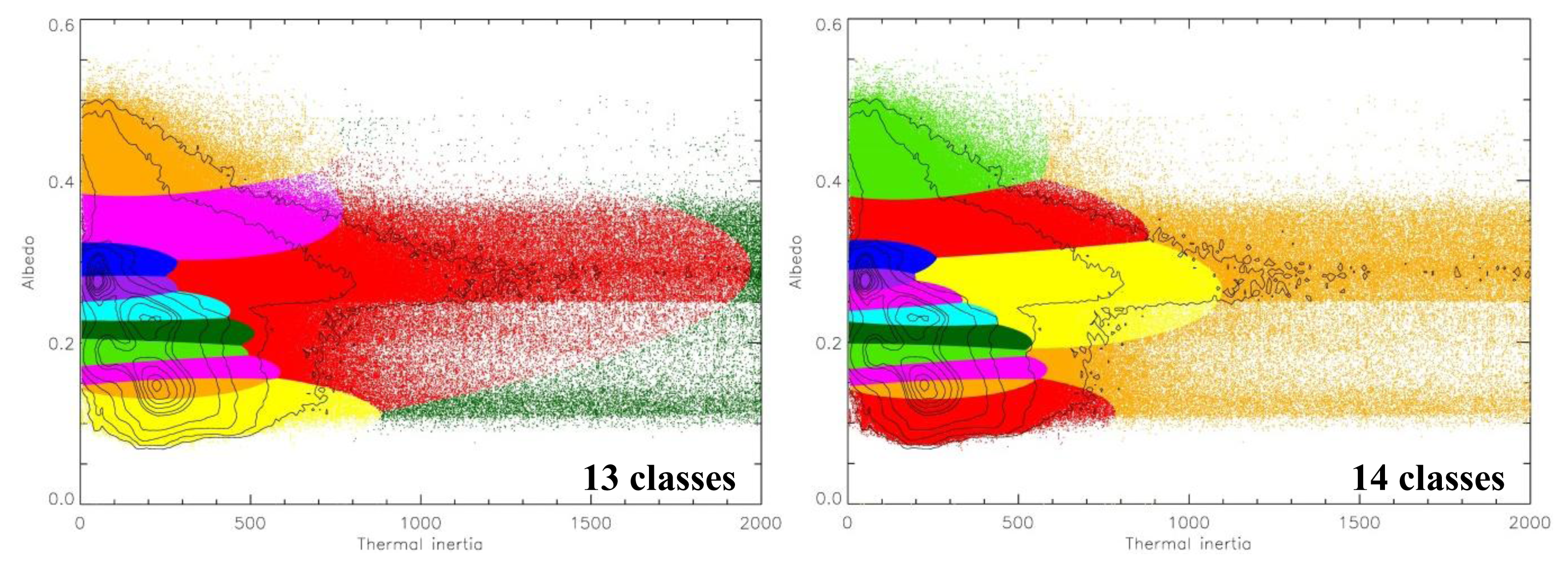
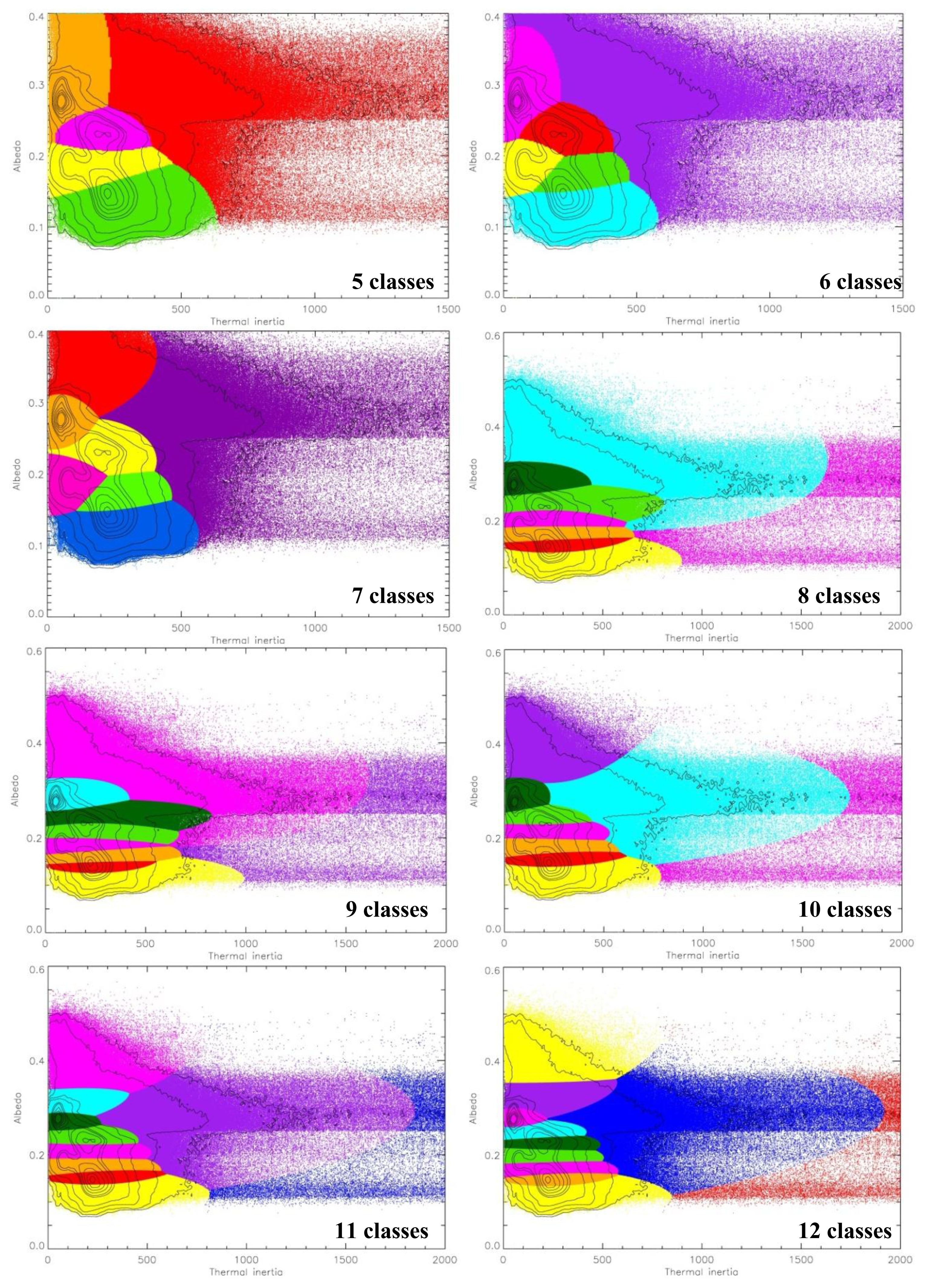
The sensitivity of the ISODATA and MAXLIKE algorithms clearly varies both with the dataset, and with the number of classes partitioned. An important result of this work is the identification of a number of factors which affect the sensitivity of these unsupervised clustering algorithms. It is essential to have an understanding of these factors prior to the application of these algorithms [154]. The assignment of pixels by the combined ISODATA and MAXLIKE algorithms is shown in Figure 6 for 5–14 classes, to compare the general behaviour of the algorithms for varying N. As the number of classes increases, more classes are generally assigned between albedo < 0.3 and thermal inertia < 700 tiu, and the boundaries of the classes are refined to better align with the underlying contours. These values encompass ~93% of the map, and correspond to surfaces dominated by dust, fine-coarse sand, indurated sand and duricrust, pebbles, and mixtures of these components (Table 1). For each value of N, at most 1/3 of the total classes are assigned to encompass values outside the aforementioned albedo and thermal inertia range, consistent with the low density of data points in that region. For some values, the resulting class boundaries appear to cross contours and split the modal peaks, thereby creating an artificial segregation of the dataspace (for example, N = 12). This can also be observed when comparing the behaviour of the algorithms on slightly different datasets. For example, in Figure 14 (older thermal inertia dataset) the low albedo/medium thermal inertia peak is clearly isolated for 5 and 6 classes, but subdivided for 4 and 7 classes. The subdivision occurs on the basis of thermal inertia, with the class boundary cross-cutting a range of albedo values. In Figure 11 (newer thermal inertia dataset), the similar low albedo/medium thermal inertia peak is again subdivided into two classes but on the basis of albedo, with the boundary cross-cutting a range of thermal inertia values. Although classification validity should be primarily determined by groundtruthing the map and comparing to independent datasets, the sensitivity of the algorithms to the dataspace clearly varies. These results illustrate the importance of carefully examining the partitioning of the dataspace by algorithmic classifiers, as their sensitivity is affected both by the structure of the underlying dataspace, and the data range of the variables in the multivariate classification problem (Figure 8).

The albedo and thermal inertia data structure shown in Figure 1, indicates that four classes can encompass the major peaks within the data, with 2–3 further classes being useful for encompassing the less frequent values in the data, e.g., (i) high thermal inertia with high albedo; (ii) mid-high thermal inertia with low-mid albedo. This suggests that 6–7 classes are sufficient to capture the major structure within the two-dimensional dataspace. However, cluster validity also depends on application [154,155], and a higher number of divisions can sometimes be justified if they provide scientifically useful information. The application of thermal inertia and albedo data in this work is to remotely map Martian surface materials and surficial geology, and for this purpose a higher number of divisions can enable more information to be extracted from the dataspace. From Figure 7, class 6 (orange) includes two peaks at high albedo (0.24 and 0.27) which correspond to a single peak in low thermal inertia (~55 tiu). From known characteristics of Martian surface materials, these pixels are likely surfaces dominated by a mantle of fine-grained dust < 10 μm across [16] which is dominating the apparent thermal inertia (Table 1). Given that complete and optically thick dust coverage results in an albedo of >0.27 [13], the two peaks in albedo within this class may indicate sub-pixel dust free regions which would be of geologic interest for spectral studies. Hence in this context, subdividing this class to produce a larger number of partitions in the dataspace would provide a more useful interpretation of surface materials.

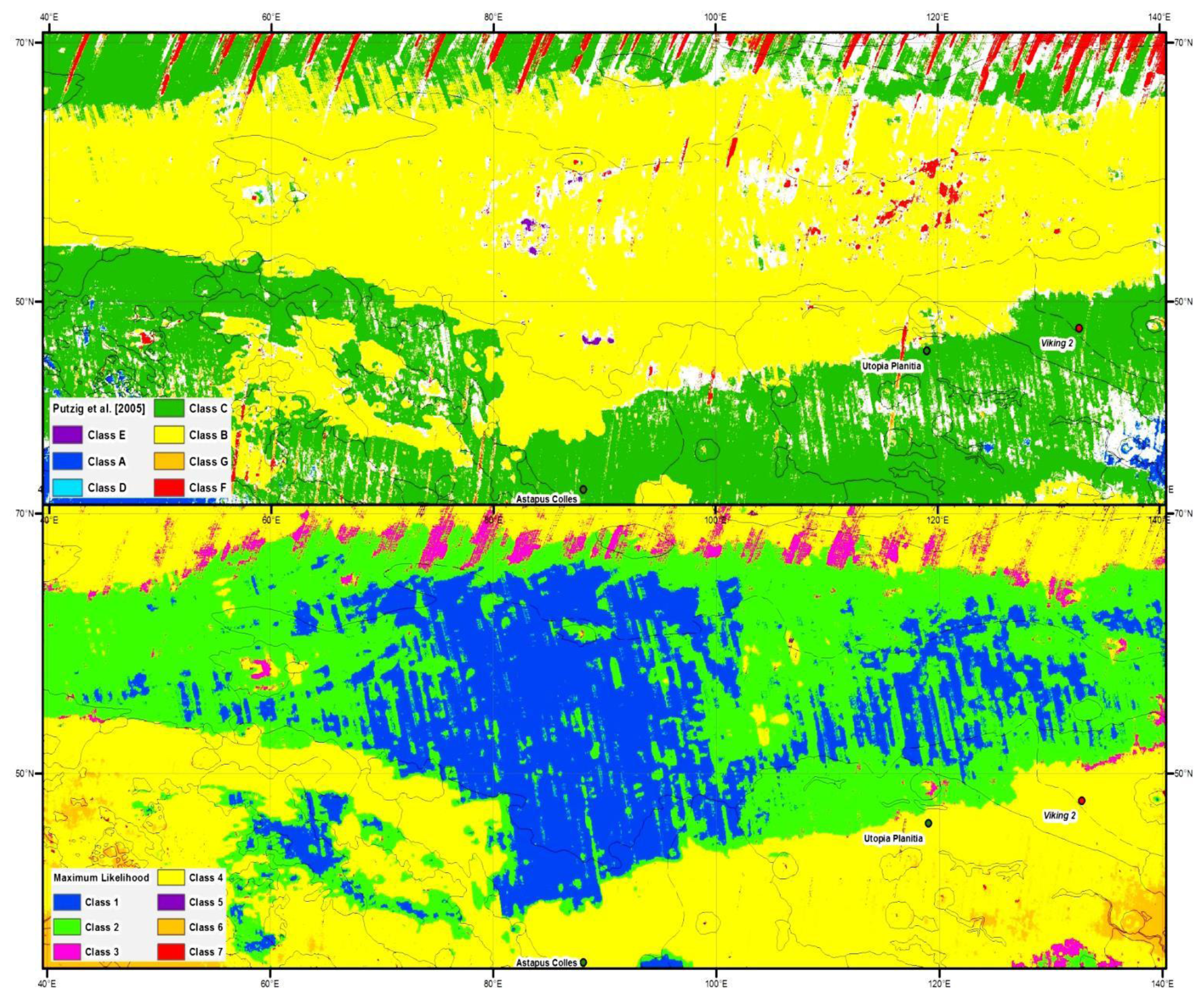
Figure 15 illustrates that some subdivisions of classes on the basis of either thermal inertia or albedo can be scientifically useful. For example, when the thermophysical classes are being applied to discriminate surfaces mantled by Martian fines and map pixels with a similar sub-pixel coverage of bright Martian dust or dark sand (Table 1). One region of difference in the spatial map of the thermophysical classes produced by [8] and that produced in this study is within Utopia Planitia. The thermal inertia values for this region (and albedo to a lesser extent) were typically higher in the newer data sets than in the data used by [8]. From Figure 15, the manual classification identifies much of the expanse of Utopia Planitia as being dominated by one major surface material (class B; yellow). In the Maximum Likelihood classification using the newer versions of thermal inertia and albedo, class 2 (green) shares a similar outer boundary to class B, however the central region of Utopia is occupied by another surface material class—class 1 (blue). The boundary between class 1 and class 2 is somewhat correlated with the geological contact mapped by [156], separating the Vastitas Borealis Formation (VBF) “mottled” (interior) and “knobby” (outer) regions. Many surface morphologies in this region are indicative of periglacial modification of the surface and a loss of past volatiles (e.g., [157,158]). The spatial correlation between class 1 and the “mottled” VBF unit highlights the usefulness of the subdivision between the green and blue classes in Figure 11.

5.1. Assessment and Validation by Comparison to Surface Features

Table 6 provides an interpretation of the thermophysical units defined in this study, by comparing the data values within each class with the known properties of Martian materials summarised in Table 1. To provide some groundtruthing of the map and the delineation of class boundaries, the interpretations are compared to surface features and geologic units.

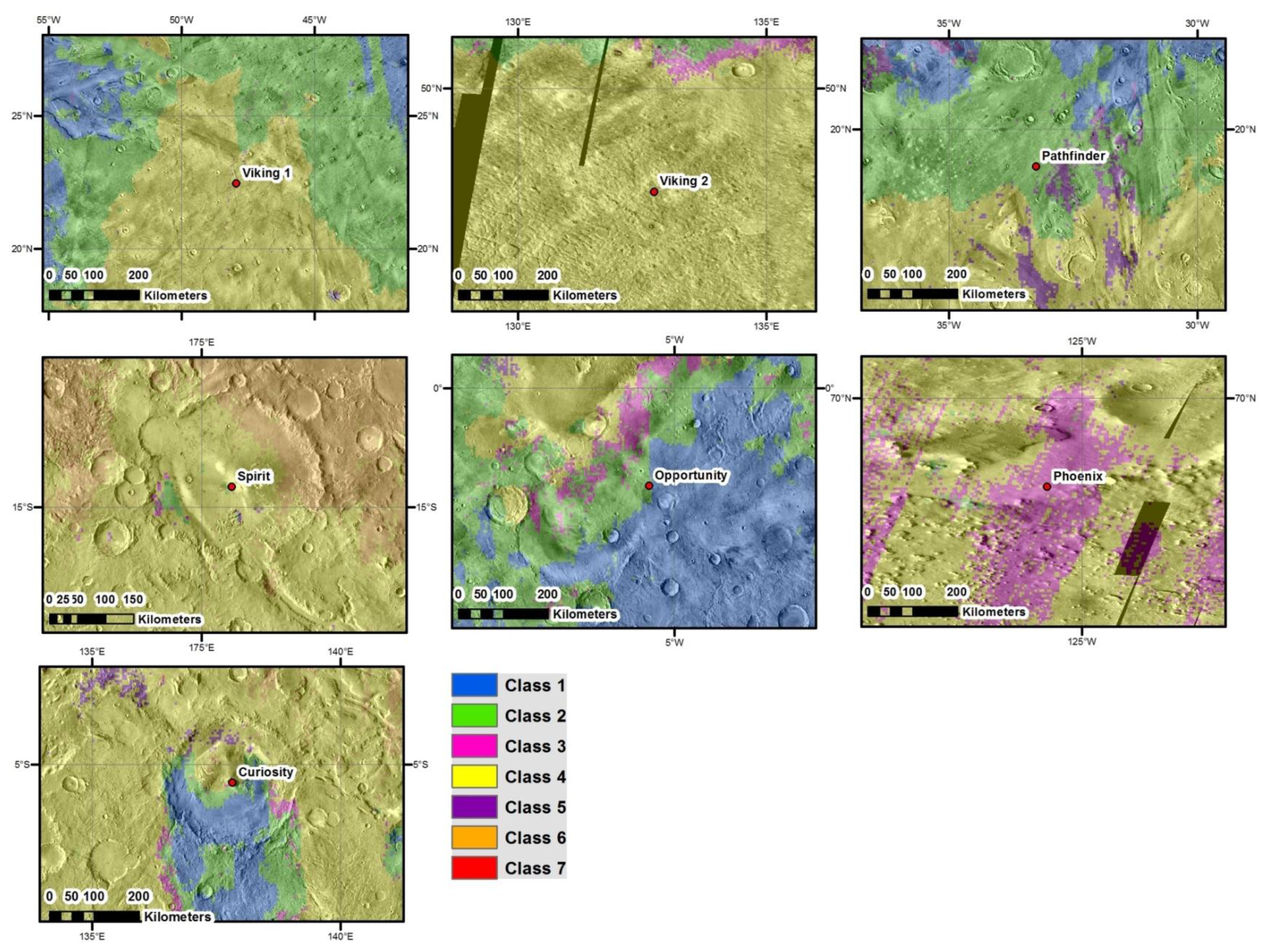
At least four of the seven thermophysical classes defined here (classes 1–4) were sampled by landers and rovers on the Martian surface (Figure 16) and hence can be groundtruthed. The results are generally consistent with the interpretation of the classes given in Table 6, with the possible exception of class 3 (fuchsia).

Class 1 (blue) terrain was sampled at Meridiani Planum by the Opportunity Rover, where the surface was found to be predominantly dust free with an albedo of 0.12 [48,159]. The terrain at Meridiani is dominated by basaltic sand and grey spherical hematite grains, millimetres in diameter [14]. Sand organised into dunes was also observed by Opportunity at Endeavour crater [160]. The high thermal inertia materials observed in the landscape were sparse rocks (400–1100 tiu) and duricrust [9,161], consistent with the interpretation in Table 6.

From Figure 11 and Table 6, class 2 (green) appears to be similar to class 1, but with a higher coverage of bright dust (higher albedo) and an overall smaller fraction of fines (low thermal inertia materials). Class 2 terrain was sampled by Pathfinder at Ares Valles, where the surface was found to be dominated by fine-grained drift material and sand [162], with ~16% of the observed area containing semi-rounded pebbles and larger rocks [163]. Dark rocks were found to have discontinuous coatings of bright red dust, raising their albedo [164]. The interpretation of grain sizes within class 2 terrain is in agreement with the fine component observed on the surface [165], as this dominates the orbital thermal inertia [10]. The Pathfinder site had the highest rock abundance of all of the landing sites [1], however there are no pixels within class 5 that have an orbital thermal inertia consistent with pebbles or larger rocks, due to the extensive sub-pixel coverage of the fine component.

Class 3 (fuchsia) terrain was sampled by the Phoenix lander in eastern Arcadia, where ice-rich soil was obscured beneath drift and dust deposits [28]. The interpretation of class 3 materials in Table 6 is consistent with the observed fine component.

Class 4 (yellow) terrain was sampled at Gusev crater by the Spirit Rover, with the surface found to be dominated by a <1 mm thick bright dust covering [48] over pebble-rich terrain and drift deposits (particles < 100 μm) [92,166]. Similar surface materials were observed by the Viking 1 lander in Chryse Planitia [20], consistent with Figure 16. Class 4 terrain was also sampled by Viking 2 at Utopia Planitia, with the surface found to be dominated by smooth fractured crusts (fragments 0.2–1.25 cm) with a fine component of crusty to cloddy material between the cracks, some rocks (centimetres to metres across), and little drift (<10 μm) material [20]. Both Viking 2 and Spirit observed a strong presence of duricrust (200–300 μm cemented grains) [2,92,166], consistent with the interpretation in Table 6.

In summary, the differences between the algorithmically defined classes in orbital thermal inertia and albedo data, have translated into observed differences on the Martian surface in the relative fractions of difference end-member materials.

Martian sand dunes predominately larger than 1 km² are being mapped from THEMIS, MOC and CTX imagery [167]. The dune boundaries can therefore be intersected with the thermophysical map to measure the overlap with different classes and test the interpretation of sand-dominated surfaces. From the ~10⁶ km² area of mapped dune coverage [168], ~86% of total dune area (normalized by class surface area) was found to occur in classes 1 (blue) and 5 (purple), shown in Figure 17. This indicates a strong correlation between large dune occurrence and surfaces interpreted as being dominated by coarse dark sand > 100 μm in Table 6. Although classes 2–4 and 6 incorporate fine-sand they have little mapped dune area, which is likely related to the required grain size for saltation driving the formation of dunes [40]. An example of a dune field in class 1 terrain is the Olympia Undae dune field [169] shown in Figure 18.

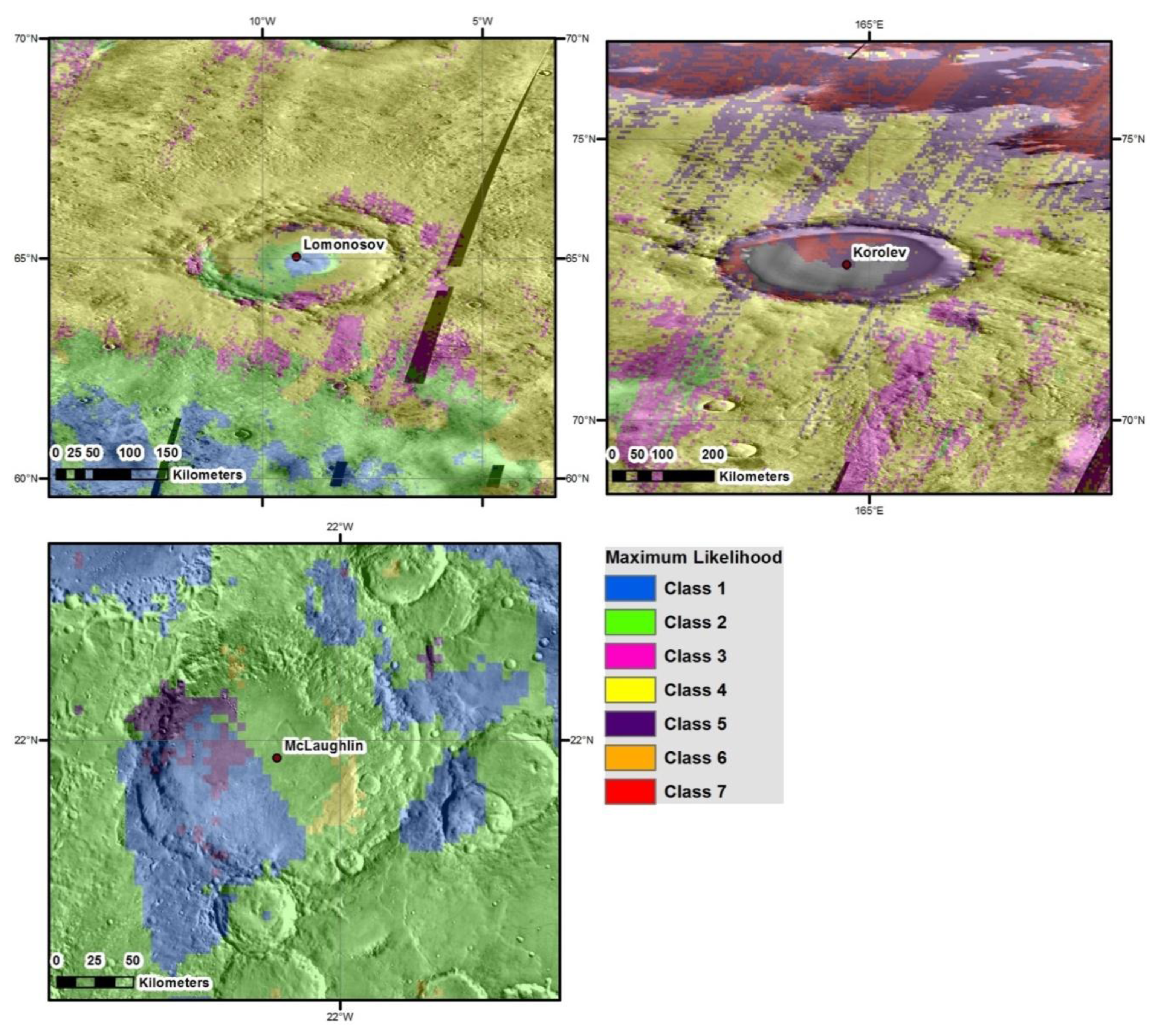
A number of impact craters with diameter over 50 km are distinguished in the thermophysical map of Figure 13. These craters can be identified by concentric circular structures of thermophysical units that contrast with the units dominating the surrounding terrain. This is consistent with observations of distinct high thermal inertia rims and impact ejecta surrounding many Martian craters [55,170]. Three interesting impact craters are shown in Figure 19. The interior of Korolev crater shows ice-related morphologies on the interior mound [171] and spectra consistent with a water ice composition [172]. From Figure 19, classes 5 and 7 infill Korolev crater and are correlated with the observed exposures of ice [173], consistent with their interpretation in Table 6.

McLaughlin crater shows evidence of a past lacustrine environment, with channels, possible debris aprons, and spectral evidence for clays and carbonates on the crater floor [175]. These features occur in the region of classes 1 and 2 terrain within the crater in Figure 19. The distribution of these materials within McLaughlin crater suggests there may be a relationship between the possibly once volatile-rich materials observed in this region and the classes 1 and 2 terrain. Additionally, other expanses of these terrains in the northern hemisphere (in Utopia and Acidalia Planitia) are correlated with extensive glacial and periglacial morphologies (e.g., [157,176]), and are modelled to have had the highest deposition of volatiles [177] during moderate obliquity (25°–35°) within the last < 10 Ma [178]. Class 4 may also be associated with subsurface volatiles, as it dominates the region visited by the Phoenix Lander in the northern arctic (Figure 16). Similarly, the interior of Lomonosov crater shows a concentric distribution of classes 1, 2, and 4 associated with its central peak and crater floor. Ice-cemented soil in Lomonosov’s interior has been speculated from thermal observations [88], and observations of seasonal water frost in the interior [179]. The distribution of class 5 material on the northern wall of Lomonosov may be associated with the observation of pure coarse CO₂ frost in this region [180], consistent with the interpretation given in Table 6 and the occurrence of class 5 in the northern polar regions.

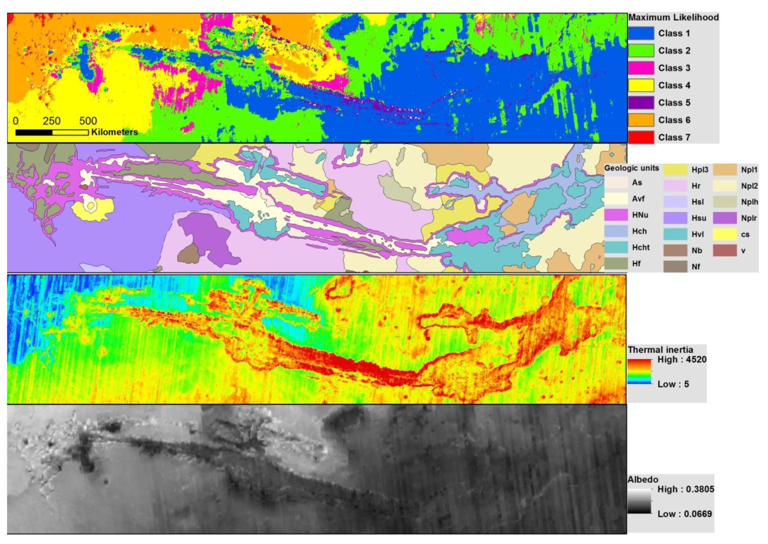
The delineation of major geologic structures such as Valles Marineris, Olympus Mons, and a number of large impact craters in the thermophysical map suggests a broad global correlation between the classes and Martian surficial geology. The Valles Marineris canyon system is shown in Figure 20. The major canyons are outlined in the geologic map by a single geologic unit (purple) and predominantly in-filled by two distinct geologic units (pale yellow and blue). In the thermophysical map, the major canyons and the western labyrinth of valleys are clearly defined by a boundary of predominately class 5 (purple), and are in-filled primarily by class 1 (blue) and class 2 (green). Several of the geologic boundaries, for example, the boundary between the low viscosity lava flows of the “ridged plains unit” and the volcanic flows of the “syria planum formation” [156,181], are also echoed in the thermophysical map. This suggests that the map may be used to resolve different types of lava flows. Furthermore, the boundaries between units in this region of the thermophysical map are not clearly identified in either the albedo map or thermal inertia map alone. Hence the division of thermophysical classes in this region provides additional information more than either dataset on its own, and is broadly correlated with boundaries of geologic units.

Martian terrain is categorized into three broad periods of geologic history based on impact crater densities, reflecting the age of the surface since its last significant reworking. The broad age bands of Noachian (surface ages 4.1–3.7 Ga), Hesperian (3.7–3.0 Ga) and Amazonian (3.0 Ga-present) [182], are each characterised by different surface processes and hence a weak relationship between surface age and grain size may be expected. Noachian surfaces, being the oldest, are heavily cratered and degraded. During this period the surface experienced extensive liquid water erosion through major flooding, such as the events that carved Valles Marineris [183] and other valley networks [184,185], and likely had long-term standing water to produce the observed sedimentary layers (e.g., [186,187]) and clay minerals [188,189]. Hesperian surfaces also experienced water activity, with outbursts of water erosion forming the outflow channels [190] and acidic water-rock interaction leading to the sulphate mineralogy [188]. Volcanic activity was frequent during this period, with extensive lava plains covering the surface [191]. 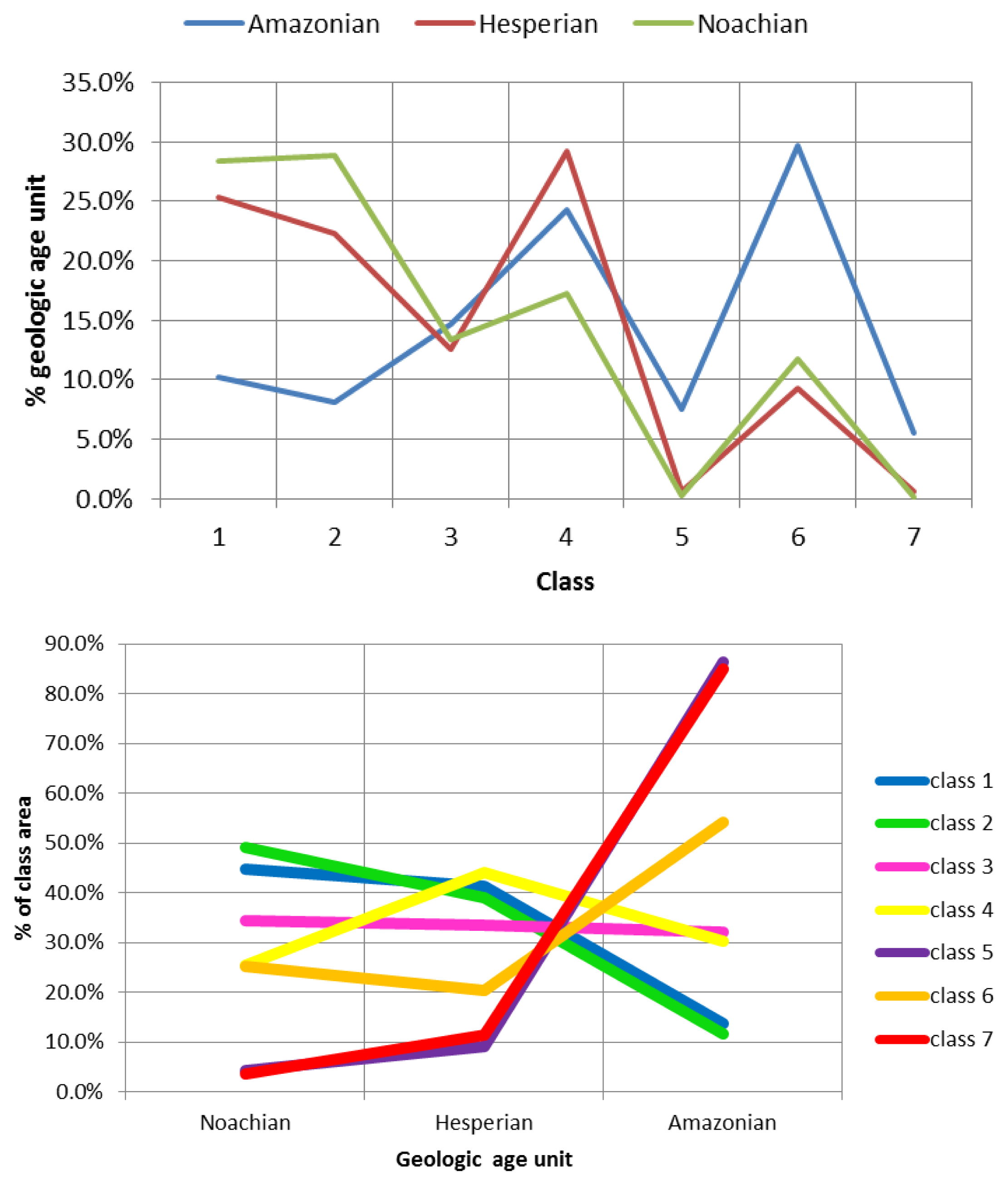The Amazonian epoch is characterized by significantly less water and lava erosion [192], with predominantly water poor environments but extensive glacial/periglacial activity [193]. The division of terrain from each of the three geologic epochs into the seven classes is shown in Figure 21. Although each class is comprised of terrain of all surface ages, there are some clear relationships between surface age and thermophysical class, when corrected for surface area. For example, Amazonian terrain predominately occurs in class 5 (purple) and 7 (red), consistent with the interpretation of surface ice in these classes obscuring the cratering record (Table 6). Class 1 (blue) and 2 (green) terrain are dominated by fines (Table 6) and are predominantly Noachian aged, consistent with the erosive action of liquid water and impact gardening increasing the fraction of fines and drifts on Noachian surfaces. No classes have a particular preference for Hesperian aged terrains.

5.2. Future Work

The above comparison of the thermophysical classes derived by the combination of ISODATA with MAXLIKE to independent datasets on Martian surface morphologies and geology, indicates that the divisions between classes translate into meaningful information on Martian surface materials. These results suggest that the unsupervised classification approach presented here can provide a powerful alternative to manual classification procedures, with new insights into Martian surficial geology.

Future work will potentially incorporate additional datasets into the classification (such as mineral maps, dayside thermal inertia, and elevation), and examine the datasets to determine the optimal number of classes for mapping thermally (and potentially mineralogically) distinct surface materials. It was noted in this work that outliers significantly affect the performance of the GMM algorithm. Hence although the algorithm appeared to have some significant limitations, it is possible that the performance could be improved by further restricting the dataspace to only include values that have a high frequency. This comes, however, at the cost of losing information on certain Martian surface materials. For example, high thermal inertia > 1000 tiu only comprise a small fraction of the dataset, but indicate surfaces with significant pebble to boulder coverage (rocks larger than ~5 mm [14,23,24,26]). In addition, the GMM has difficulty in reproducing pixel counts, typically overestimating by a factor of >2. Given the analysis within this work, the combined use of ISODATA and MAXLIKE is recommended for any future work on unsupervised partitioning of these datasets.

6. Conclusions

This work focused on comparing the classifications of thermal inertia and albedo data by the Expectation Maximisation of a Gaussian Mixture Model, Iterative Self-Organizing Data Analysis Technique, and Maximum Likelihood algorithms, to identify which classifier provides greatest sensitivity to the underlying dataspace. The factors which affected the performance and sensitivity of each algorithm were examined. This analysis was motivated by the continued importance of characterizing the thermophysical properties of the Martian surface at ~3 km resolution. In particular, the need for rigorous mapping of surficial geology and grain sizes to provide constraints for future landing sites and to develop our understanding of the geologic processes that have shaped the Martian surface. The MAXLIKE classifier paired with ISODATA was found to be generally more sensitive to the data structure than both ISODATA on its own and EM of a GMM. This was illustrated through the generally lower spread of values within the classes and the sensitivity in fitting the global thermal inertia and albedo histogram. The seven thermophysical classes derived were groundtruthed against several independent datasets suitable for determining classification validity, including comparisons with surface data from lander missions, geologic maps, and features derived from imagery. The resultant classifications were shown to correspond to meaningful variations in surface materials. Motivation was provided for a finer partitioning of the thermal inertia and albedo dataspace, in combination with other independent datasets, to be undertaken in future.