Blending Landsat and MODIS Data to Generate Multispectral Indices: A Comparison of “Index-then-Blend” and “Blend-then-Index” Approaches

Abstract

The objective of this paper was to evaluate the accuracy of two advanced blending algorithms, Spatial and Temporal Adaptive Reflectance Fusion Model (STARFM) and Enhanced Spatial and Temporal Adaptive Reflectance Fusion Model (ESTARFM) to downscale Moderate Resolution Imaging Spectroradiometer (MODIS) indices to the spatial resolution of Landsat. We tested two approaches: (i) “Index-then-Blend” (IB); and (ii) “Blend-then-Index” (BI) when simulating nine indices, which are widely used for vegetation studies, environmental moisture assessment and standing water identification. Landsat-like indices, generated using both IB and BI, were simulated on 45 dates in total from three sites. The outputs were then compared with indices calculated from observed Landsat data and pixel-to-pixel accuracy of each simulation was assessed by calculating the: (i) bias; (ii) R²; and (iii) Root Mean Square Deviation (RMSD). The IB approach produced higher accuracies than the BI approach for both blending algorithms for all nine indices at all three sites. We also found that the relative performance of the STARFM and ESTARFM algorithms depended on the spatial and temporal variances of the Landsat-MODIS input indices. Our study suggests that the IB approach should be implemented for blending of environmental indices, as it was: (i) less computationally expensive due to blending single indices rather than multiple bands; (ii) more accurate due to less error propagation; and (iii) less sensitive to the choice of algorithm.

1. Introduction

Trade-offs between acquisition frequency and spatial resolutions of satellite image data are inherent in all single-sensor satellites [1]. In the last decade, several advanced blending algorithms have been developed to combine data observed from multiple sensors with various spatial resolutions and temporal densities (e.g., Landsat, Medium Resolution Imaging Spectrometer (MERIS), Moderate Resolution Imaging Spectroradiometer (MODIS) and Advanced Very High Resolution Radiometer (AVHRR)). Gao et al. [2] developed the Spatial and Temporal Adaptive Reflectance Fusion Model (STARFM) algorithm to blend surface reflectance from two sensors to simulate more frequent higher spatial resolution surface reflectance output (e.g., Landsat-like imagery at the frequency of MODIS acquisition). Zhu et al. [3] enhanced the STARFM algorithm (denoted ESTARFM) to improve the model spatial variability of heterogeneous study sites. Both algorithms are widely used by the remote sensing community ([1] their

Table 3. Bands and band-widths of Landsat TM and corresponding MODIS bands.

Landsat TM a Band/Band Name	Landsat TM Band-Width (nm)	MODIS Band/Band Name	MODIS Band-Width (nm)
Band 1/Blue	450–520	Band 3/Blue	459–479
Band 2/Green	520–600	Band 4/Green	545–565
Band 3/Red	630–690	Band 1/Red	620–670
Band 4/NIR	760–900	Band 2/NIR	841–876
Band 5/SWIR1	1550–1750	Band 6/SWIR1	1628–1652
Band 7/SWIR2	2080–2350	Band 7/SWIR2	2105–2155

^aThe ETM+ band-widths are slightly different from TM band-widths. The ETM+ characteristic are reported in Chandler et al. ([36], Table 4).

).

The objective of much blending research is to simulate reflectance data from which multispectral indices can be calculated, such as vegetation and water indices at a high spatial resolution and temporal density [4–8]. Vegetation indices are widely used to effectively characterize particular biophysical or biochemical properties and processes for vegetated surfaces [9]. The Normalized Difference Vegetation Index (NDVI; [10]) and the Enhanced Vegetation Index (EVI; [9]), are the most common satellite-derived indices used by the remote sensing community for monitoring vegetation at regional to global scale for numerous applications [11–14]. The Simple Ratio (SR) is best used for estimating Leaf Area Index (LAI; [15]). There are also several environmental moisture indices that are commonly used, including: (i) Global Vegetation Moisture Index (GVMI; [16]); and (ii) Depth of 1650 nm relative to a reference continuum line determined at 835 nm and 2208 nm (D₁₆₅₀; [17]). Water indices, such as the Normalized Difference Water Index (NDWI) are also widely used to delineate open water features and enhance their presence in satellite images. The NDWI [18] has been used by researchers in its original and modified forms (

Table 1. List of nine indices and their equations used here. NIR, SWIR1 and SWIR2 are abbreviations for Near-Infrared, Shortwave-Infrared1 and Shortwave-Infrared2 bands, respectively. Except for Enhanced Vegetation Index (EVI), Simple Ratio (SR) and Depth of 1650 nm (D₁₆₅₀), all indices use a normalized difference formulation generically given as (band x − band y)/(band x + band y), where x and y represent bands.

Index Name	Bands Used	# Bands Used	Theoretical Range	Equation
NDVI	Red, NIR	2	[−1.0, +1.0]	$(\text{NIR}-\text{Red})/(\text{NIR}+\text{Red})$
EVI	Blue, Red, NIR	3	[0.0, +1.0]	$2.5\times (\text{NIR}-\text{Red})/(\text{NIR}+6\times \text{Red}-7.5\times \text{Blue}+1)$
SR	Red, NIR	2	[0.0, → ∞]	$\text{NIR}/\text{Red}$
GVMI	NIR, SWIR1	2	[−0.82, 0.96]	$\left((\text{NIR}+0.1)-(\text{SWIR}1+0.02)\right)/\left((\text{NIR}+0.1)+(\text{SWIR}1+0.02)\right)$
D1650	NIR, SWIR1, SWIR2	3	[→ −∞, +1.0]	$1-\left(\frac{\text{SWIR}1}{\text{NIR}\times \left(1-0.59359\right)+0.59659\times \text{SWIR}2}\right)$
NDWI24	Green, NIR	2	[−1.0, +1.0]	$\left(\text{Green}-\text{NRI}\right)/\left(\text{Green}+\text{NRI}\right)$
NDWI25	Green, SWIR1	2	[−1.0, +1.0]	$\left(\text{Green}-\text{SWIR}1\right)/\left(\text{Green}+\text{SWIR}1\right)$
NDWI27	Green, SWIR2	2	[−1.0, +1.0]	$\left(\text{Green}-\text{SWIR}2\right)/\left(\text{Green}+\text{SWIR}2\right)$
NDWI45	NIR, SWIR1	2	[−1.0, +1.0]	$\left(\text{NIR}-\text{SWIR}1\right)/\left(\text{NIR}+\text{SWIR}1\right)$

). An example includes the modified version of NDWI (MNDWI of [19]), which uses the Shortwave-Infrared (SWIR1) band (i.e., Landsat TM band 5) in place of the Near-Infrared (NIR) band (i.e., Landsat TM band 4). The selected nine indices are the most widely used subset of remotely sensed indices from the: (i) vegetation domain; (ii) environmental moisture domain; and (iii) water domain.

Many recent studies using STARFM first blend reflectance from Landsat and MODIS data and then use these outputs to calculate vegetation or water indices (e.g., [4,6–8,20,21]). Herein, we refer to this process as Blend-then-Index (BI), with the alternative approach being Index-then-Blend (IB). For the IB approach, the indices were calculated first and these indices were input into the blending algorithms to simulate indices at the date of simulation. For the BI approach, reflectance bands were input into the blending algorithms to simulate reflectance, which was used as input to calculate multispectral indices. In the IB approach we assume that a linear mixture model is applicable to indices (i.e., the mixed index for each MODIS pixel is the sum of the index weighted by the class area proportions), as it is for the reflectance bands. According to Kerdiles and Grondona [22] this assumption introduces very small errors to statistics when using indices directly into a linear mixture model (i.e., IB) instead of using individual band reflectance data in the model (i.e., BI). In the only previous study to compare IB with BI, Tian et al. [23] evaluated the accuracy of STARFM for simulating a time series of 12 NDVI images over a single study site. Our paper extends that study by: (i) using both the STARFM and ESTARFM algorithms; (ii) using three sites with contrasting spatial and temporal dynamics; (iii) calculating nine commonly used indices in vegetation, environmental moisture and standing water applications; and (iv) partitioning the spatial and temporal variances to explain the results. The aims of our paper are to: (i) comprehensively examine if one of the approaches (i.e., IB versus BI) consistently outperforms the other for a range of vegetation, environmental moisture and standing water indices; (ii) explore whether spatial and temporal variances are related to the blending accuracy of indices by the two algorithms (i.e., STARFM versus ESTARFM); and (iii) isolate the impact that the approach or algorithm has on blending accuracy (i.e., approach versus algorithm). These three aims provide the structure of our paper and are used as subheadings in the Methods, Results and Discussion sections.

2. Materials

2.1. Study Site and Data Sets

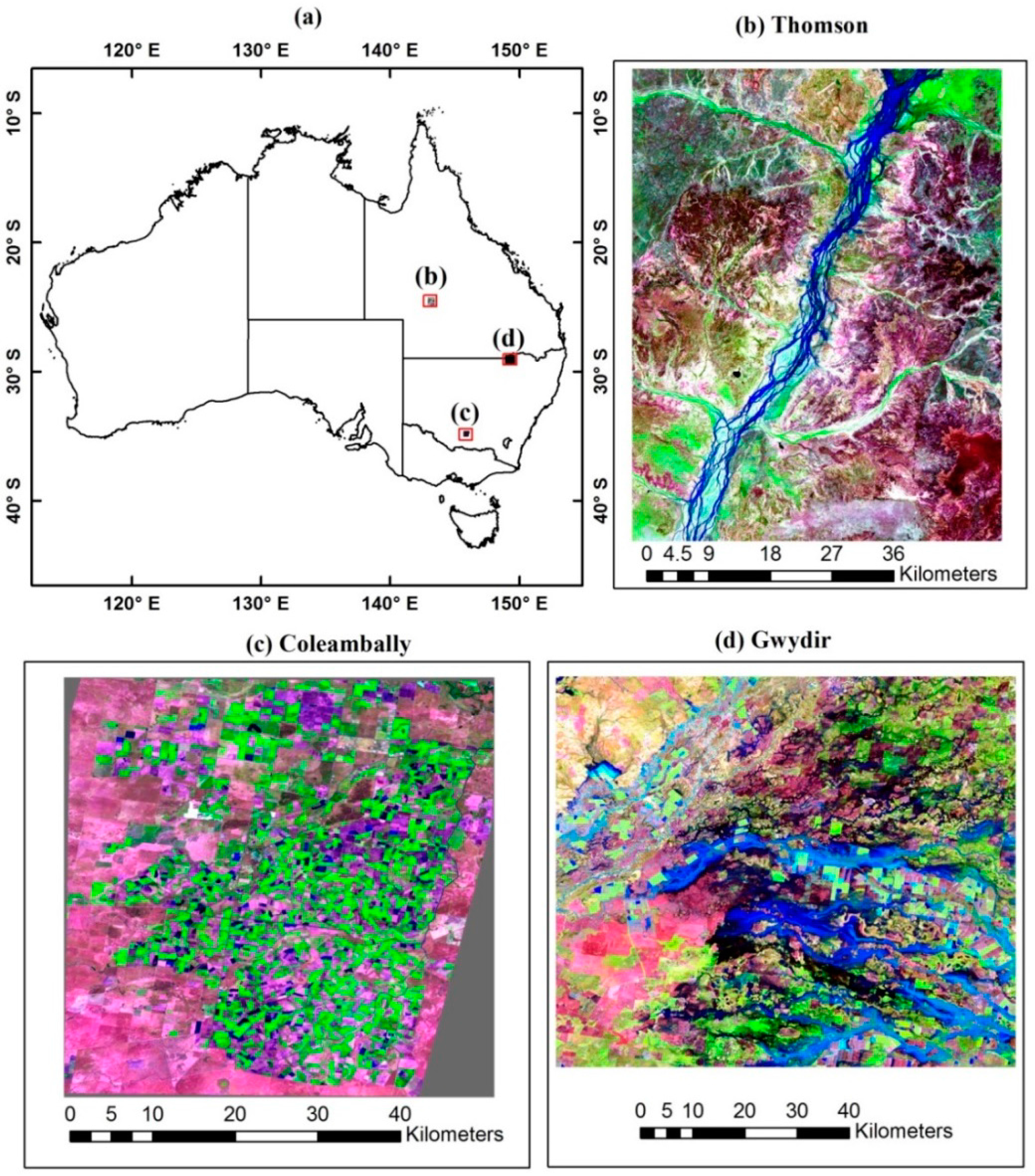
Three study sites with different relative spatial and temporal variances and different land cover patch sizes were selected in this study (Figure 1); they are introduced in turn. The Thomson River floodplain study site (Thomson herein) is an extensive anabranching river system located in central Queensland, Australia (143.20°E, 24.50°S, see Figure 1). The Thomson study site covers 3850 km² (55 km E–W × 70 km N–S) within a Landsat-5 TM scene (path 96, row 77). The Thomson site is located in the Lake Eyre Basin in a region called the “Channel Country”, which is characterized by extensive floodplains and a complex anabranching river system with ephemeral flows following precipitation [24,25]. It has a low topographic gradient and dynamic land cover in watercourses and floodplains [25,26]. Its Köppen-Geiger climate is in the arid (B), steppe (S) and hot (h) zone, with a mean annual temperature greater than 18 °C [27]. The land use in the Lake Eyre Basin is dominated by grazing. Mitchell Grass plains, sand dunes, spinifex grasslands, gibber deserts, stony plains and acacia woodlands are landscapes of the Cooper Creek catchment [28]. The flooding is the only water source for flora and fauna of the area, and there is a distinct greening up following the passage of floodwaters.

The Coleambally Irrigation Area study site (Coleambally from herein) is a rice based irrigation system located in southern New South Wales (NSW, Australia; 34.0034°E, 145.0675°S). Standing water associated with flood irrigation of summer rice fields is present in October and November [17,29,30]. Summer crop development (i.e., rice, soybeans, corn and sorghum—the last three crops being furrow irrigated) occurs from December to April, with many crops harvested by May. The surrounding dryland agricultural areas mainly have a winter growing season (cereals and pasture), and several small residual woodland patches in the northern part of the images are fairly constant throughout the time series.

The Lower Gwydir Catchment study site (Gwydir from herein) is located in northern NSW (149.2815°E, 29.0855°S). The temporal extent of data over the Gwydir was greater than one year, and included a winter and a summer crop-growing season. The Gwydir, which covers the typical dual growing season crop phenology and surrounding dryland agricultural area, experienced a large flood in mid-December 2004. This flooding, and subsequent inundation, occupied a large spatial extent of the Gwydir imagery and was temporally very dynamic (Figure 1). The Gwydir site is spatially more homogenous than the Coleambally and Thomson sites, because of the larger agricultural fields, coupled with the large (and quick) flooding event. The flooding/inundation at Gwydir was a significant test of the blending algorithms in conditions with extremely high spatio-temporal variability.

For Thomson, 20 pairs of cloud-free Landsat-MODIS (L–M) images were used from April 2008–October 2011 (

Table 2. Dates of cloud-free Landsat-5 and Terra Moderate Resolution Imaging Spectroradiometer (MODIS) images from 2008–2011 for Thomson. The bold row indicates the image captured during major flood event (Image # 11, see Figure 1b).

Image #	Date	Day since Start of Dataset (15 April 2008)	MODIS Sensor Zenith (Degree)
1	15 April 2008	0	13.26
2	22 September 2008	160	13.29
3	24 October 2008	192	13.51
4	17 March 2009	336	13.62
5	2 April 2009	352	13.42
6	24 August 2009	496	13.37
7	9 September 2009	512	13.28
8	25 September 2009	528	13.39
9	11 October 2009	544	13.57
10	12 September 2010	880	13.27
11	2 January 2011	992	12.85
12	19 February 2011	1040	12.86
13	8 April 2011	1088	12.86
14	10 May 2011	1120	13.43
15	13 July 2011	1184	13.65
16	29 July 2011	1200	13.74
17	14 August 2011	1216	13.86
18	30 August 2011	1232	13.90
19	15 September 2011	1248	13.19
20	1 October 2011	1264	13.25

). This period was characterized by an intense La Niña, and major flooding occurred over much of eastern and central Australia in 2009 and 2010, during which large areas were covered with standing water. The most likely time to observe standing water at this site is during the wet season, from November–April. Between 2008 and 2011 most of the Landsat and/or MODIS images were cloudy during January and February. After selecting all cloud-free inundated images during the wet season, the other images were selected to be as close as possible to when the inundated images were acquired (Table 2). The Coleambally site images were Landsat 7. The Thomson and Gwydir sites images were Landsat 5 data and were corrected for Bidirectional Reflectance Distribution Function (BRDF) effects. The Gwydir images were corrected using the Li et al. [31] BRDF algorithm. The Thomson images were corrected to at-surface reflectance using the Flood et al. [32] BRDF algorithm (also taking into account atmospheric conditions, topography, sensor location and sun elevation) using the parameterized bi-directional reflectance model for eastern Australia [32]. All MODIS data were BRDF corrected Terra MODIS Collection 5, daily reflectance (MOD09GA) images with 500 m pixels for all bands [33]. MODIS data, which were originally processed by the Land Processes Distributed Active Archive Center (LPDAAC) at the U.S. Geological Survey (USGS) Earth Resources Observation and Science Center (EROS), were obtained from The Commonwealth Scientific and Industrial Research Organization (CSIRO) Marine and Atmospheric Research Division.

For detailed information about the other two study sites, Coleambally and Gwydir, see [1]. Briefly, 17 L–M image pairs acquired over eight months for Coleambally and 14 L–M image pairs acquired over 12 months at Gwydir were used. Partitioning the variance into its spatial and temporal components [1] showed that Coleambally reflectance data had higher spatial variance (than temporal variance) and more accurate results were obtained with ESTARFM due to its design. In contrast, at Gwydir temporal variance dominated spatial variance and due to algorithmic assumptions STARFM worked best. Finally, Coleambally has a smaller effective patch size than Gwydir [1]. The three study sites have different relative spatial and temporal variances and different patch sizes, governing the area-to-perimeter ratio within the different resolution imagery used in the blending algorithms. These three sites are purposefully selected to form a continuum between solely man-made standing water and entirely natural standing water: (i) at Coleambally all standing water is man-made (due to irrigation); (ii) at Gwydir both irrigated fields and standing water associated with flooding are present, and (iii) at Thomson standing water is only associated with flooding. The dynamics and area-to-perimeter ratios of standing water (and associated responses) varied across the three sites, and these three sites are therefore a robust selection from which to evaluate performance within and between both blending algorithms across the IB and BI approaches.

2.2. Data Pre-Processing

A Landsat–like image was generated on a given simulation date by using a total of five input images, being two L–M pairs (one before and one after the simulation date) and the MODIS image on the simulation date as input to either STARFM or ESTARFM [1]. The observed Landsat image on the date of simulation was preserved for validation and was not used as input to the blending algorithms. Herein, the date of simulation is denoted t₂, the first L–M pair date will be referred to as t₁ and the date of the second L–M pair is indicated as t₃. For example, at Thomson, L–M pairs from 15 April 2008 (t₁) and 24 October 2008 (t₃) and the MODIS image on 22 September 2008 (t₂) were used to create a Landsat-like image on 22 September 2008 (t₂), see Table 2. At Thomson, a total of 18 Landsat-like images were simulated in this manner using the nearest temporal neighboring L–M pairs to the central dates listed in Table 2 as image #’s 2–19, herein referred to as “3-sequential date images”. Observed MODIS images were resampled to Landsat resolution using the nearest neighbor approach and the five Landsat or MODIS images involved in any given blending operation were then co-registered based on a correlation test [1]. The co-registration results of Terra MODIS images in this study confirm the along-track and along-scan band-to-band co-registration error in Terra MODIS bands [34]. The optimal spatial offset to maximize the correlation between corresponding bands of L–M images was calculated by using the IDL (Exelis Visual Information Solutions, Boulder, Colorado) code developed by NASA [35] and applied to MODIS images.

We used the six reflective Landsat bands and the corresponding MODIS bands for the blending algorithms (Table 3). All nine indices (i.e., NDVI, EVI, SR, GVMI, D₁₆₅₀, NDWI₂₄, NDWI₂₅, NDWI₂₇ and NDWI₄₅, see Table 1) were calculated for all Landsat and MODIS images at each site. All simulated indices (from both approaches) were compared with the observed Landsat indices at date t₂. Then all nine indices were calculated and compared with indices calculated from the observed Landsat images at date t₂.

2.3. Blending Algorithms

STARFM and ESTARFM assume that images from different sensors are acquired under similar land surface conditions and that surface reflectance is comparable after pre-processing [3]. The STARFM algorithm can use either one pair or two pairs of L–M images (i.e., dates t₁ and/or t₃) and one low resolution image (date t₂) to simulate a high resolution image at date t₂, while the ESTARFM algorithm uses two pairs of L–M images (i.e., dates t₁ and t₃) and one low resolution image (date t₂) to simulate date t₂. For STARFM we use the two L–M image pair option to have consistent input with ESTARFM.

The algorithms identify spatial changes of reflectance from the high spatial resolution images by finding spectrally similar neighbor pixels and temporal changes from the low-resolution images to simulate the high spatial resolution and high temporal density images at selected dates. A moving search window (w) is used to select similar neighboring pixels, and heterogeneity of the landscape is considered by the number of land cover classes in each pixel of the low resolution image [3]. The algorithms use weight factors for each spectrally similar pixel to blend temporal and spatial information. Proximal to the central pixel and spectrally similar fine resolution pixels have higher weights [3]. To make the result comparable with former studies, here the size of w was 50 by 50 Landsat resolution pixels and the assumed number of spectrally-different classes was four. STARFM is able to model non-linear changes between two Landsat images and would be expected to model temporal variability better than ESTARFM. In contrast, ESTARFM has been designed to work better in more spatially heterogeneous areas [1,2].

3. Methods

3.1. IB versus BI

The accuracy of the STARFM and ESTARFM algorithms for simulating all nine Landsat-like indices was assessed by comparing the bias (calculated as observed minus simulated), correlation coefficient of determination (R²) and Root Mean Square Deviation (RMSD) between the simulated and observed Landsat indices, using both the IB and BI approaches. Additionally, the results from the IB and BI approaches for both blending algorithms were examined by comparing temporally mean bias, R² and RMSD across the entire blended dataset for each site (18 dates for Thomson, 15 dates for Coleambally and 12 dates for Gwydir; there are two less instances than the number of images available at each site due to using the blending algorithms with L–M pairs before and after each simulation date).

The paired t-test was used to assess if the difference of the mean error between the IB and BI approaches was statistically significant. Mean error between IB and BI for each “3-sequential date image” was paired. The assessment was performed for both the STARFM and ESTARFM algorithms, for each of the three sites, and for each of the three above-mentioned error statistics at the 90% (i.e., p < 0.1) and 95% (i.e., p < 0.05) confidence levels. For example using STARFM at Thomson, the mean bias of each of the 18 simulated images generated using IB were paired to the corresponding 18 mean biases generated using BI to test whether the biases between IB and BI were statistically significant. This example was extended to all combinations of error statistics, sites and algorithms.

3.2. STARFM versus ESTARFM

Quantification of spatial and temporal variances of image and index time series, given the strengths and weaknesses of each algorithm, is an important step toward selecting blending algorithms [1]. Here we used the same method ([37], their Equation 10) to partition the grand (or spatio-temporal) variance into the spatial and temporal variance components and assessed the suitability of STARFM and ESTARFM. Following [1], we calculated spatial and temporal variances of each possible combination of 3-sequential dates of the high and low resolution images. The temporal to spatial variances ratio (T/S), as an indicator of algorithm selection, was also calculated for each 3-sequential dates of L–M bands and indices. This was performed for all six reflective bands and nine indices of L–M images at Thomson. Since the temporal and spatial variances were already reported for Coleambally and Gwydir for the bands [1], here we only report the indices’ variances for these two sites. The paired t-test was used to assess if the difference of the mean error between the STARFM and ESTARFM algorithms was statistically significant, using the general technique as previously explained.

3.3. Approach versus Algorithm

To compare and quantify the impact of the IB versus BI approaches on the accuracy of STARFM versus ESTARFM, R² and RMSD statistics were calculated for four parameters (i.e., (STARFM-ESTARFM)_IB, (STARFM-ESTARFM)_BI, (IB-BI)_STARFM and (IB-BI)_ESTARFM). To quantify STARFM versus ESTARFM for the IB approach, differences between STARFM and ESTARFM statistics; (STARFM–ESTARFM)_IB; were calculated and averaged for all 405 simulations (nine indices by 45 dates—the total from the three sites). For the BI approach, a similar parameter; (STARFM-ESTARFM)_BI; was also calculated. To quantify IB versus BI, averaged difference R² and RMSD statistics were calculated across all 405 simulations (as above) using the STARFM algorithm; (IB-BI)_STARFM; and ESTARFM algorithm; (IB-BI)_ESTARFM.

4. Results

4.1. IB versus BI

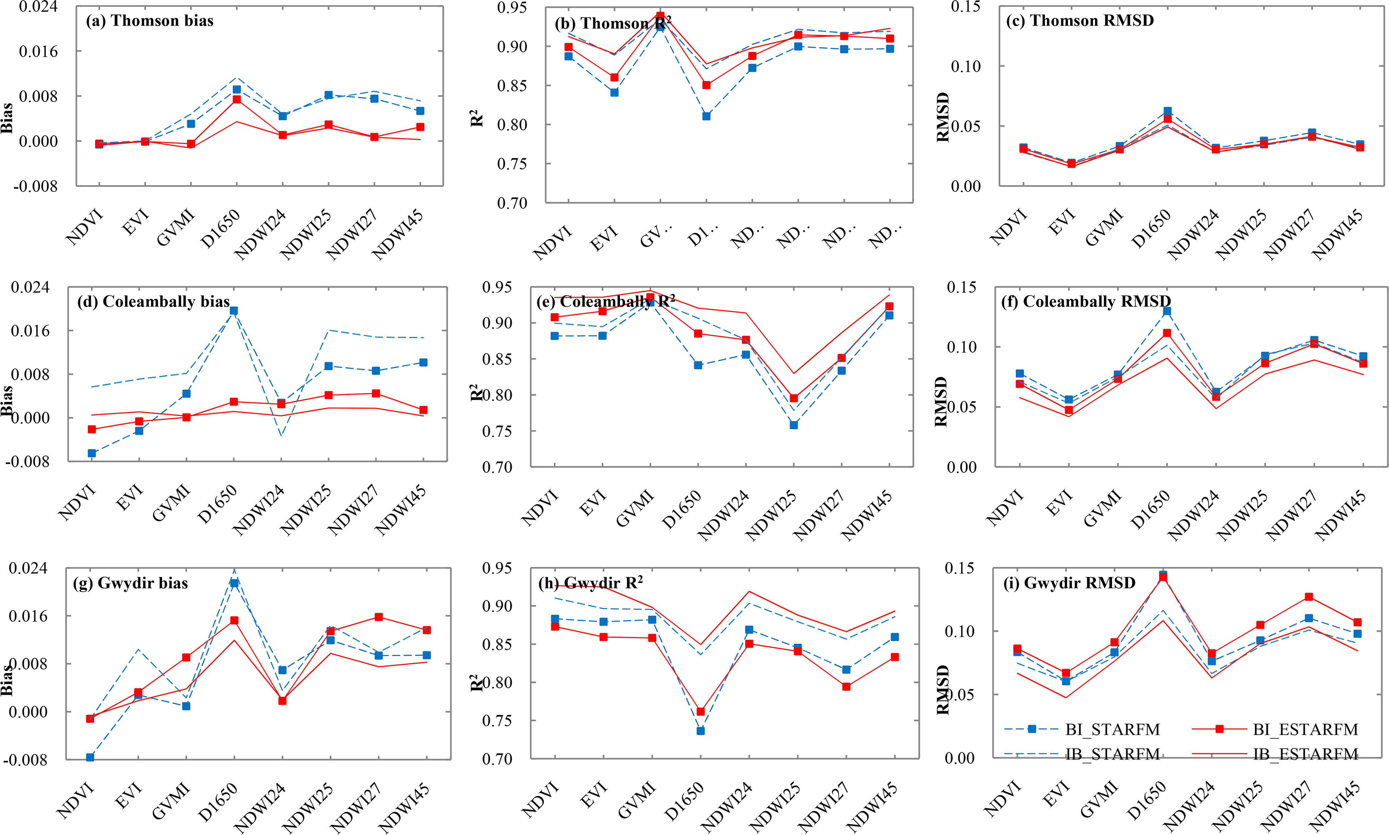
The statistics (

Table 4. Mean bias, R² and root mean square deviation (RMSD) statistics between the observed and simulated index values from Spatial and Temporal Adaptive Reflectance Fusion Model (STARFM) and Enhanced Spatial and Temporal Adaptive Reflectance Fusion Model (ESTARFM) for the both the Index-then-Blend (IB) and Blend-then-Index (BI) approaches for Thomson, Coleambally and Gwydir, which are abbreviated as T, C and G respectively in the column headings. Bias and RMSD are presented in index units.

Indices	Bias						R2						RMSD
	STARFM			ESTARFM			STARFM			ESTARFM			STARFM			ESTARFM
	T	C	G	T	C	G	T	C	G	T	C	G	T	C	G	T	C	G
IB-NDVI	−0.0003	0.0057	−0.0013	−0.0008	0.0005	−0.0008	0.92	0.90	0.91	0.91	0.94	0.93	0.0278	0.0709	0.0747	0.0284	0.0576	0.0667
BI-NDVI	−0.0006	−0.0065	−0.0076	−0.0005	−0.0021	−0.0012	0.89	0.88	0.88	0.90	0.91	0.87	0.0321	0.0778	0.0835	0.0310	0.0691	0.0862
IB–EVI	0.0000	0.0071	0.0104	0.0000	0.0011	0.0018	0.89	0.89	0.90	0.89	0.94	0.93	0.0160	0.0531	0.0602	0.0160	0.0418	0.0475
BI-EVI	−0.0001	−0.0024	0.0028	−0.0001	−0.0007	0.0032	0.84	0.88	0.88	0.86	0.92	0.86	0.0193	0.0562	0.0605	0.0185	0.0475	0.0671
IB-SR	0.0086	0.1838	0.2658	0.0024	0.0250	0.0943	0.90	0.87	0.88	0.91	0.90	0.90	0.1245	1.3270	1.4802	0.1179	1.2051	1.6800
BI-SR	0.0028	0.1781	0.1392	0.0011	0.0796	0.0813	0.88	0.85	0.87	0.90	0.87	0.80	0.1346	1.3799	1.4005	0.1291	1.2874	1.6800
IB-GVMI	0.0048	0.0081	0.0023	−0.0013	0.0003	0.0038	0.93	0.93	0.90	0.94	0.94	0.90	0.0311	0.0749	0.0797	0.0299	0.0682	0.0764
BI-GVMI	0.0030	0.0044	0.0009	−0.0005	0.0001	0.0091	0.92	0.93	0.88	0.94	0.94	0.86	0.0333	0.0769	0.0833	0.0305	0.0734	0.0913
IB-D1650	0.0114	0.0050	0.0018	0.0034	−0.0003	0.0027	0.87	0.91	0.88	0.88	0.93	0.89	0.0507	0.0303	0.0272	0.0492	0.0269	0.0271
BI-D1650	0.0092	0.0043	0.0013	0.0074	0.0001	0.0041	0.81	0.90	0.85	0.85	0.92	0.82	0.0626	0.0315	0.0301	0.0559	0.0284	0.0339
IB-NDWI24	0.0048	−0.0034	0.0035	0.0010	0.0004	0.0020	0.90	0.88	0.90	0.90	0.91	0.92	0.0281	0.0569	0.0666	0.0283	0.0485	0.0630
BI-NDWI24	0.0044	0.0027	0.0069	0.0011	0.0025	0.0018	0.87	0.86	0.87	0.89	0.88	0.85	0.0317	0.0625	0.0763	0.0305	0.0584	0.0826
IB-NDWI25	0.0076	0.0161	0.0144	0.0023	0.0018	0.0097	0.92	0.78	0.88	0.91	0.83	0.89	0.0339	0.0936	0.0879	0.0347	0.0773	0.0902
BI-NDWI25	0.0082	0.0095	0.0119	0.0029	0.0042	0.0135	0.90	0.76	0.85	0.91	0.80	0.84	0.0377	0.0925	0.0927	0.0348	0.0864	0.1049
IB-NDWI27	0.0088	0.0148	0.0099	0.0007	0.0018	0.0075	0.92	0.85	0.86	0.91	0.89	0.87	0.0407	0.1032	0.1008	0.0414	0.0891	0.1034
BI-NDWI27	0.0075	0.0086	0.0094	0.0007	0.0045	0.0158	0.90	0.83	0.82	0.91	0.85	0.79	0.0445	0.1057	0.1103	0.0411	0.1026	0.1270
IB-NDWI45	0.0072	0.0147	0.0141	0.0003	0.0003	0.0083	0.92	0.92	0.89	0.92	0.94	0.89	0.0314	0.0869	0.0906	0.0306	0.0770	0.0845
BI-NDWI45	0.0053	0.0102	0.0094	0.0025	0.0015	0.0136	0.90	0.91	0.86	0.91	0.92	0.83	0.0347	0.0922	0.0979	0.0322	0.0861	0.1069

) showed that for all nine indices examined, the IB approach outperformed the BI approach at all three sites. The paired t-test analysis showed that the means of the three abovementioned error statistics produced for the three sites of “3-sequential date images” for the two approaches were statistically different at the 95% confidence interval in 65% of the STARFM and 53% of the ESTARFM cases (

Table 5. t-test results to assess approaches and algorithms are statistically different. Probability of <0.05 is shown in the italic and bold font, and probability <0.1 are provided as italic, >0.1 is normal font. Last two rows show number of cases with <0.05 and <0.1 probabilities and their percentage (count/18 × 100) in brackets. Under the ‘Approach’ headings, testing differences due to IB or BI, statistics for the first grouping of the nine indices use STARFM and the second grouping of nine use ESTARFM. Under the ‘Algorithm’ headings, testing differences due to blending algorithms, statistics for the first grouping use the IB approach and the second grouping use the BI approach. Thomson, Coleambally and Gwydir are abbreviated as T, C and G, respectively.

Indices	Bias						R2						RMSD
	Approach			Algorithm			Approach			Algorithm			Approach			Algorithm
	T	C	G	T	C	G	T	C	G	T	C	G	T	C	G	T	C	G
NDVI	0.835	0.000	0.000	0.882	0.000	0.001	0.001	0.251	0.204	0.835	0.003	0.011	0.000	0.353	0.935	0.987	0.003	0.026
EVI	0.773	0.000	0.009	0.714	0.001	0.710	0.002	0.044	0.037	0.669	0.001	0.006	0.000	0.050	0.015	0.736	0.000	0.020
SR	0.130	0.860	0.337	0.015	0.001	0.280	0.024	0.000	0.000	0.172	0.000	0.000	0.042	0.378	0.293	0.195	0.077	0.603
GVMI	0.120	0.001	0.208	0.002	0.000	0.744	0.030	0.003	0.101	0.033	0.000	0.829	0.043	0.015	0.104	0.511	0.000	0.501
D1650	0.239	0.842	0.743	0.000	0.000	0.003	0.000	0.000	0.000	0.327	0.010	0.265	0.000	0.000	0.000	0.166	0.002	0.155
NDWI24	0.561	0.002	0.086	0.000	0.018	0.552	0.000	0.008	0.009	0.649	0.002	0.037	0.000	0.011	0.001	0.916	0.001	0.069
NDWI25	0.450	0.002	0.620	0.000	0.001	0.279	0.002	0.193	0.000	0.308	0.008	0.181	0.002	0.772	0.020	0.675	0.035	0.375
NDWI27	0.413	0.010	0.887	0.000	0.000	0.742	0.005	0.105	0.000	0.428	0.013	0.283	0.016	0.532	0.000	0.666	0.029	0.522
NDWI45	0.076	0.003	0.113	0.000	0.000	0.040	0.010	0.004	0.004	0.494	0.005	0.489	0.006	0.010	0.003	0.539	0.002	0.224
NDVI	0.939	0.188	0.579	0.975	0.056	0.873	0.093	0.004	0.004	0.116	0.001	0.211	0.069	0.000	0.009	0.354	0.000	0.161
EVI	0.821	0.057	0.849	0.837	0.000	0.104	0.357	0.000	0.000	0.253	0.001	0.352	0.248	0.000	0.000	0.453	0.001	0.495
SR	0.784	0.032	0.798	0.571	0.001	0.311	0.169	0.000	0.002	0.099	0.092	0.016	0.140	0.047	1.000	0.296	0.050	0.067
GVMI	0.585	0.832	0.347	0.001	0.000	0.411	0.226	0.000	0.010	0.000	0.004	0.285	0.673	0.000	0.005	0.003	0.006	0.354
D1650	0.076	0.321	0.454	0.019	0.000	0.238	0.012	0.000	0.000	0.000	0.000	0.177	0.004	0.000	0.000	0.001	0.000	0.825
NDWI24	0.935	0.057	0.936	0.000	0.787	0.187	0.521	0.000	0.002	0.098	0.001	0.249	0.393	0.000	0.000	0.381	0.009	0.135
NDWI25	0.610	0.244	0.236	0.000	0.001	0.881	0.818	0.000	0.000	0.000	0.002	0.753	0.981	0.003	0.000	0.000	0.011	0.049
NDWI27	0.981	0.181	0.242	0.000	0.025	0.676	0.951	0.000	0.000	0.000	0.018	0.202	0.892	0.000	0.000	0.000	0.096	0.071
NDWI45	0.180	0.536	0.216	0.000	0.000	0.611	0.279	0.001	0.004	0.016	0.004	0.216	0.347	0.000	0.003	0.002	0.006	0.358
Count<0.05	0(0)	8(44)	2(11)	13(72)	16(89)	3(17)	10(56)	15(83)	16(89)	6(33)	17(94)	5(28)	10(56)	13(72)	14(78)	5(28)	15(83)	3(17)
Count<0.1	2(11)	10(56)	3(17)	13(72)	17(94)	3(17)	11(61)	15(83)	16(89)	8(44)	18(100)	5(28)	11(61)	14(78)	14(78)	5(28)	18(100)	6(33)

). The higher accuracy of the IB approach is most likely explained by error propagation, as the IB approach only incurs one instance of blending so there is only one process where blending-induced error can be introduced. In contrast, the BI approach incurs multiple blending instances and therefore multiple instances of error that subsequently propagates to the resultant indices. Moreover, for those indices having a normalized difference formulation (i.e., NDVI, GVMI, NDWI₂₄, NDWI₂₅, NDWI₂₇ and NDWI₄₅, see Table 1) their algebra reduces error.

At the Thomson site, comparing the R² of the blended indices with those calculated from observed Landsat data revealed that the IB approach resulted in higher accuracy than the BI approach in 89% of 162 (9 indices by 18 dates) STARFM simulations and 75% of ESTARFM simulations (Figure 2). The three averaged error statistics for the 18 STARFM and ESTARFM indices were statistically different at the 90% confidence level (bias; 11% of the cases, R²; 61% of the cases and RMSD; 61% of the cases, Table 5). The sign of the average bias produced by STARFM overestimated (negatively-biased) 32% of 162 simulations and ESTARFM overestimated 51% of all simulations by the IB approach. Comparing the nine indices showed that site-averaged simulated NDVI and EVI produced lowest bias in all four options compared with other indices due to use of red and infrared bands. ESTARFM results overestimated NDVI, EVI and GVMI and underestimated SR, D₁₆₅₀, NDWI₂₄, NDWI_25, NDWI₂₇ and NDWI₄₅ (Table 4). Statistics derived using the BI approach have higher spatial variances during the wet season (December–March) of each year; especially during the major flood event on date 2 January 2011 (date 992). As was found for the IB approach, most of the 162 BI simulations were underestimated by STARFM (62%) and ESTARFM (53%). The NDVI and EVI values were overestimated by STARFM for the BI approach, while the NDVI, EVI and GVMI indices were overestimated by ESTARFM at Thomson (Table 4).

At Coleambally, from all 135 (nine indices by 15 dates) simulations, 90% produced higher accuracy by the IB approach when using STARFM and 98% when using ESTARFM (Figure 2). Using the paired t-test the IB and BI approaches were statistically different when comparing means of statistics (bias; for 56% of the cases, R²; for 83% of the cases and RMSD for 78% of the cases) at the 90% confidence level (Table 5). When using IB the site-averaged bias in ESTARFM was lower compared with STARFM as shown for BI approach (Figure 2). The STARFM algorithm overestimated NDWI₂₄ and underestimated all other indices when using IB, while NDVI and EVI indices were overestimated by both STARFM and ESTARFM algorithms approach and other seven indices were underestimated by using BI. From all 135 simulations, 27% and 50% are overestimated when using STARFM and ESTARFM, respectively, using the IB approach. By using BI, STARFM overestimated 36% and ESTARFM overestimated 48% of the simulations in Coleambally.

At Gwydir, the IB approach outperformed the BI by producing higher R² in 90% of all 108 (nine indices by 12 dates) simulations when using STARFM, and 100% of all simulations when using ESTARFM (Figure 2). The IB and BI approaches were statistically different at the 90% confidence level when comparing means of statistics (bias; 18%, R²; 89%, RMSD; 78%; see Table 5). STARFM underestimated 71% of 108 simulations and ESTARFM underestimated 57% of all 108 simulations when using the IB approach. When using the BI approach 41% were overestimated by STARFM and 40% were overestimated by ESTARFM. Site-averaged NDVI was overestimated and the other eight indices were underestimated by using either STARFM or ESTARFM when using IB and BI approach (Table 4). STARFM produced higher mean bias compared with ESTARFM for all nine indices when using IB and BI approach at Gwydir.

The IB approach also produced a lower RMSD (higher accuracy) at all three sites for both STARFM (Thomson; 89%, Coleambally; 81% and Gwydir; 82%) and ESTARFM (Thomson; 70%, Coleambally; 94% and Gwydir; 98%). The mean bias, R² and RMSD statistics for each site are presented in Figure 2. As shown in Figure 2a,c, Thomson had lower mean bias and RMSD statistics for all nine indices compared with Coleambally and Gwydir, because of its lower spatio-temporal variances (Section 4.2). The results for each index at each site presented in Figure 2 and Table 4 are the site-averaged statistics from all 3-sequential date simulations. The performance of STARFM and ESTARFM in each individual simulation is likely to be different from these averaged results.

Results (Table 4) showed that both STARFM and ESTARFM algorithms simulated indices with higher bias and RMSD and lower R² for dates with higher spatial and temporal variances (Section 4.2). For example, high temporal and spatial variances at date 992 for Thomson, due to inundation of the river channel, and at date 192, most likely due to changes in soil surface moisture and seasonal vegetation changes, resulted in lower accuracies when simulating all nine indices.

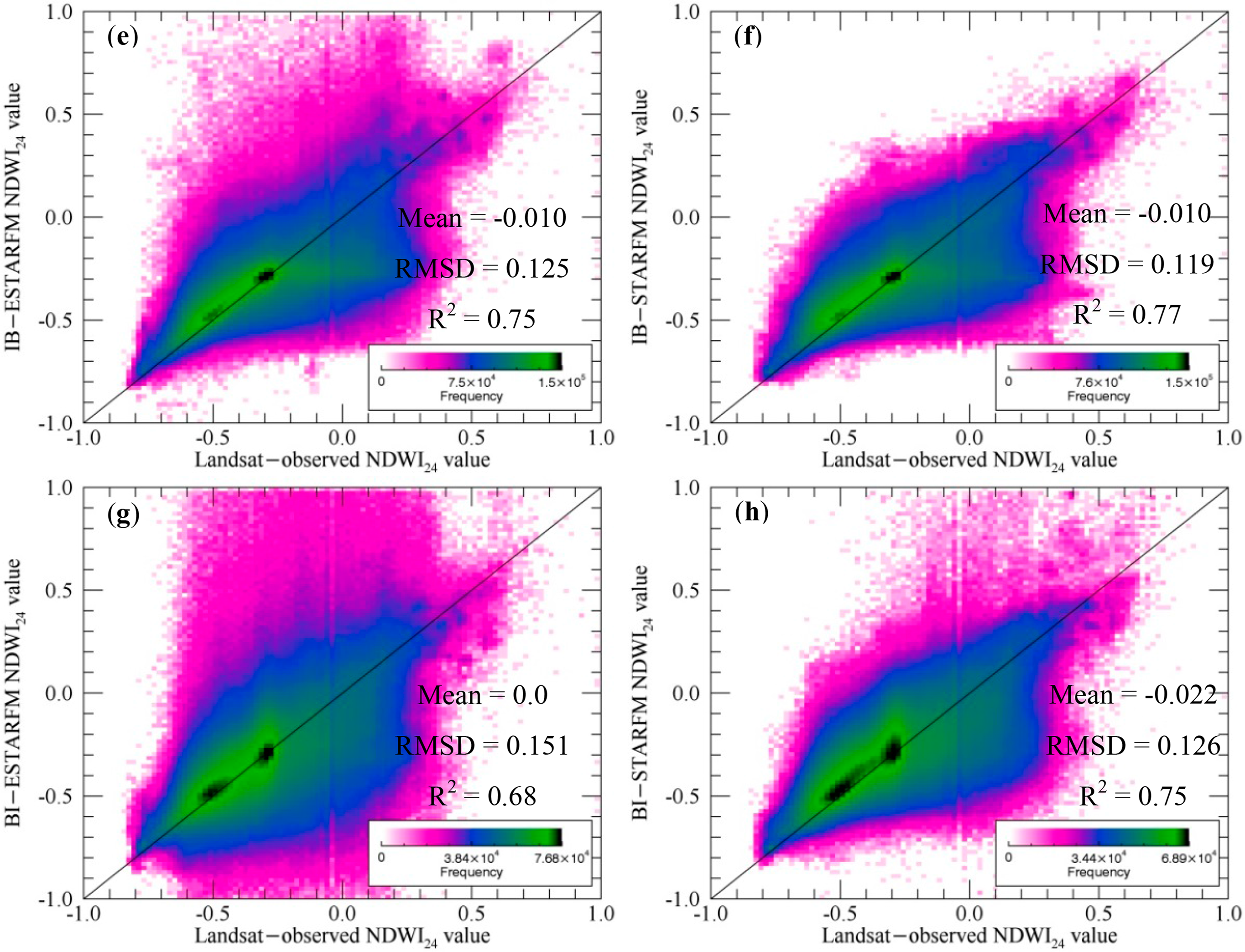
As an example, Figure 3 compares bias and R² statistics for NDWI₂₄ of Gwydir simulated by the IB and BI approaches by STARFM and ESTARFM at the flood date on 12 December 2004. As shown in Figure 3, IB outperformed BI when using either STARFM or ESTARFM. On this date STARFM produced higher accuracy (higher R² and lower RMSD and bias) compared with ESTARFM due to higher T/S variances ratio by a flood event, which is in agreement with the algorithm selection criteria proposed by [1]. Higher biases were shown in highly variable inundated areas of Gwydir by both STARFM and ESTARFM (Figure 3a,b,c,d).

4.2. STARFM versus ESTARFM

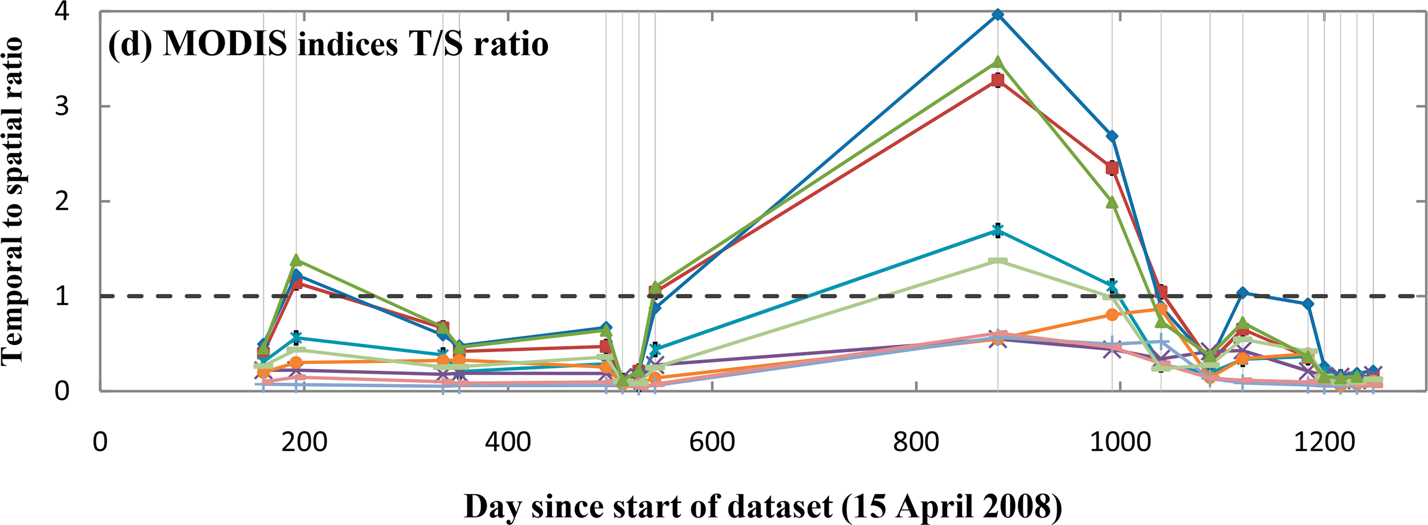
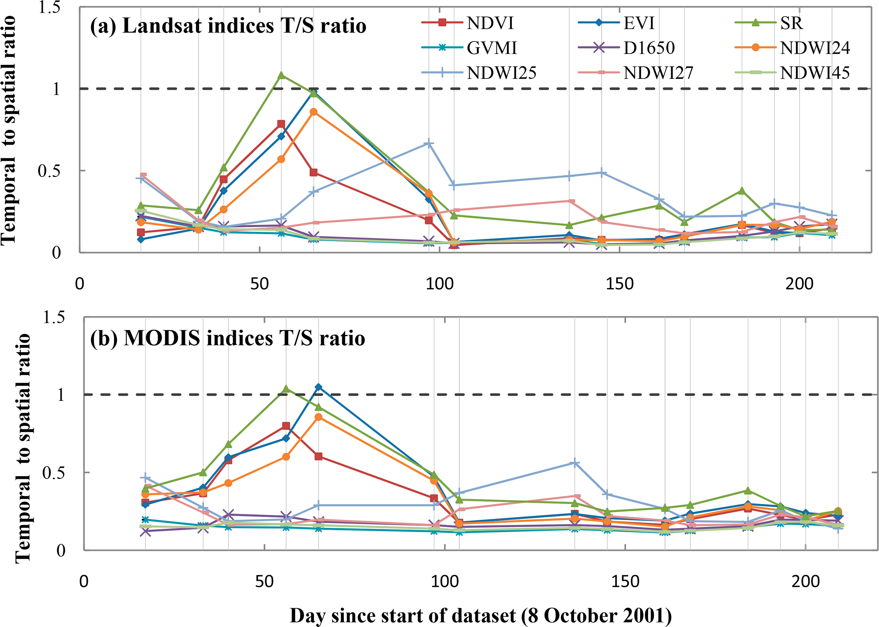
Performance of STARFM and ESTARFM algorithms in simulating IB and BI indices was related to the T/S variances ratio. STARFM showed higher accuracy in simulating all nine indices at dates with higher T/S ratio of Thomson, Coleambally and Gwydir. In contrast, ESTARFM produced better simulations at dates with lower T/S ratio (Table 4). Comparing the statistics also showed that all nine indices produced different T/S ratio by using similar inputs, therefore, even on a certain date, there is no single optimum algorithm (STARFM or ESTARFM) for all nine indices. For example, on date 880 at Thomson, the T/S ratio of NDVI and EVI were higher than the other indices (Figure 4), which resulted in higher R² and lower RMSD in simulating these indices by STARFM. Alternately, the other indices, which had lower T/S ratios, produced higher accuracies by ESTARFM. Higher temporal variance resulted when any 3-sequential date image set contained highly dynamic land-cover change (e.g., associated with flood events). For example the Thomson flood event (date 992) resulted in higher T/S variances ratio at dates 880, 992 and 1040 (Figure 4). The site-averaged spatio-temporal variance results were smaller for Thomson (0.015) than Coleambally (0.784) and Gwydir (1.610). The highly variable (river channel and floodplain) portion of Thomson imagery is relatively small compared to the surrounding low variance portion of that imagery (Figure 1), whereas in both Coleambally and Gwydir the highly variable portions of the imagery were relatively larger, being relatively largest for Gwydir (Figure 1).

At Thomson, ESTARFM produced slightly higher accuracies than those yielded from STARFM for both IB and BI approaches. Using the paired t-test the ESTARFM and STARFM approaches were statistically different when comparing means of statistics (bias; for 72% of the cases, R²; for 44% of the cases and RMSD for 28% of the cases) at the 90% confidence level (Table 5). Similar to findings for Coleambally and Gwydir reported by [1], at Thomson the T/S variances ratio of Bands 7 and 5 were the dominant variances in both Landsat and MODIS resolutions followed by Band 4, Band 3, Band 2 and Band 1 (Figure 4a,b). This is due to selecting hydrologically active sites (in all cases). For all six bands through the entire time series results showed that spatial variance was greater than temporal variances (T/S < 1, Figure 4a,b), which means the area is more variable in space than in time. Temporal variances of all six Landsat bands were lower than corresponding MODIS bands. In contrast, spatial variances of Landsat bands were higher than spatial variances of the corresponding MODIS bands; most likely because of the lower spatial resolution. Landsat bands showed higher spatio-temporal variances compared with MODIS bands. Comparison of the spatial and temporal variances of indices through the dataset showed that the magnitude of spatial and temporal variances depends on the magnitude of the indices (Figure 4). For example, SR had highest averaged spatio-temporal variance followed by NDWI₂₇, D₁₆₅₀, GVMI, NDWI₂₅, NDWI₄₅, NDVI, NDWI₂₄ and EVI (Figure 4c,d). Distinct changes in the spatial and temporal variances occurred during the flood (date 992) and at the point of transition between the dry and wet seasons (dates 1088 and 1120) due to increased precipitation and water flow in the multi-channel river system and consequent vegetation growth. Normalized indices calculated from bands with diverse spectral regions showed higher spatial and temporal variances compared with other indices calculated from bands with similar spectral regions. For example, NDWI₂₇ and NDWI₂₅ water indices, which use SWIR1 and NIR bands, had higher spatio-temporal variances when compared with other water indices, i.e., NDWI₂₄ and NDWI₄₅ (Figure 4). EVI showed the highest T/S ratio followed by SR, NDVI, NDWI₂₄, NDWI₄₅, GVMI, D₁₆₅₀, NDWI₂₅ and NDWI₂₇ (Figure 4c,d). Vegetation indices showed a higher T/S ratio due to higher changes in greenness of the study site after precipitation and corresponding rapid vegetation growth. Comparing Landsat and MODIS variances revealed that all nine Landsat indices had higher temporal, spatial and spatio-temporal variances than the MODIS indices in Thomson.

At Coleambally, with moderate spatio-temporal changes and lower T/S ratio for all dates (Figure 5), ESTARFM produced better results than STARFM by using both IB and BI approaches. IB-ESTARFM produced the most accurate results (0.82 < R² < 0.95) followed by BI-ESTARFM (0.80 < R² < 0.94), IB-STARFM (0.78 < R² < 0.93) and BI-STARFM (0.76 < R² < 0.93). The three averaged error statistics for the 18 STARFM and ESTARFM indices were statistically different at the 90% confidence level (bias; 94% of the cases, R²; 100% of the cases and RMSD; 100% of the cases, Table 5). All nine indices showed lower temporal variances compared with spatial variances in both Landsat and MODIS resolutions (Figure 5). Date 97 was a transition date at Coleambally: for all dates before date 97, higher temporal and lower spatial variances of NDWI_24, NDVI and EVI resulted in a higher T/S ratio compared with the other indices. In contrast for dates after 97, these indices showed lower T/S ratios (Figure 5). Rice was the dominant crop at Coleambally. Dates 0 through 97 were when rice fields were flooded, rice was planted and the crop grew to full canopy closure. During this time of active plant growth, the T/S ratio was higher for the three indices that make use of the visible and NIR bands when compared to the indices that make use of the longer wave bands. SR had the highest averaged spatio-temporal variance followed by D₁₆₅₀, NDWI₄₅, GVMI, NDWI_27, NDVI, NDWI₂₅, EVI and NDWI₂₄ (Figure 5). SR showed the highest T/S ratio followed by EVI, NDWI_24, NDVI, NDWI₄₅, NDWI₂₇, D₁₆₅₀, NDWI₂₅ and GVMI (Figure 5). Comparing Landsat and MODIS variances revealed that, all nine Landsat indices had temporal, spatial and spatio-temporal variances that were higher than the MODIS indices in Coleambally.

At the highly temporally dynamic Gwydir with higher T/S ratio at few selected dates, averaged statistics of all simulations showed that ESTARFM produced better results than STARFM by using the IB approach (Figure 2). By using the BI approach, STARFM produced better results than ESTARFM (Figure 2h,i). The STARFM and ESTARFM approaches were statistically different at the 90% confidence level when comparing means of statistics (bias; 17%, R²; 28%, RMSD; 33%; see Table 5).

Gwydir had higher temporal variances overall than the other two sites while non-normalized SR and normalized NDWI₂₅ and NDWI₂₇ produced higher temporal variances than the other six indices. At dates 208, 240 and 256, temporal variance was higher than spatial variance resulting in higher T/S ratios at these dates compared with other dates (Figure 6). The T/S ratios of dates 128, 288, 304, 320 and 336 were lower than the other dates due to lower temporal variances and higher spatial variances (Figure 6). SR had the highest averaged spatio-temporal variance followed by D₁₆₅₀. SR and D₁₆₅₀ are not normalized difference indices (Table 1), so they do not benefit from error reduction due to their formulation like the normalized difference indices do (as discussed in Section 4.1). SR produced the least accurate results as it is unbounded, so when the dominator → 0 then SR →∞, hence possibly producing large relative errors. Furthermore, D₁₆₅₀ uses three bands (NIR, SWIR1 and SWIR2), while other moisture indices (i.e., GVMI and NDWI₄₅) only use two of these three bands. This increases the likelihood of higher error propagation in D₁₆₅₀. For these reasons, the R² statistic for both SR and D₁₆₅₀ improved most when using IB compared to BI at Gwydir where the variance was highest due to extreme flood-related moisture dynamics. This suggests that using the IB approach might be even more important when the index is not a normalized difference index. The EVI is also not a normalized difference index using three bands (like D₁₆₅₀) but two of these are visible bands which have much lower variances than the NIR and SWIR bands [1], so the EVI produces lower errors.

SR showed the highest T/S ratio followed by EVI, D₁₆₅₀, NDWI_45, NDVI, GVMI, NDWI₂₄, NDWI₂₇, and NDWI₂₅ (Figure 6). Comparing Landsat and MODIS variances revealed that all nine Landsat indices had higher temporal, spatial and spatio-temporal variances than the MODIS indices due to lower spatial resolution of MODIS compared with Landsat.

All presented results in Figure 2 and Table 4 are site-averaged and do not show results of individual simulations. As an example here in Figure 7, we presented individual statistics for all 12 simulations of NDWI₂₅ of Gwydir by using STARFM and ESTARFM and two IB and BI approaches. As shown on Figure 7, on dates with a higher T/S ratio (i.e., date 256), STARFM outperformed ESTARFM by producing higher R² and lower RMSD and bias compared with other dates.

4.3. Approach versus Algorithm

Comparing the R² and RMSD of four parameters, that is (STARFM-ESTARFM)_IB, (STARFM-ESTARFM)_BI, (IB-BI)_STARFM and (IB-BI)_ESTARFM, revealed that the differences between statistics of the IB and BI approaches in both algorithms were greater than STARFM and ESTARFM statistics by using both approaches. This means improvement in accuracy of simulations by selecting the right approach (IB) is more important and produces higher simulation accuracies than selecting the right algorithm. It was shown that using the IB approach improved the average R² by 0.4% when using STARFM and 3.7% when using ESTARFM. ESTARFM improved the average R² by 4.6% when using the IB approach and 1.2% when using the BI approach. Using the IB approach lowered the RMSD by 12.8% when using STARFM and by 16% when using ESTARFM compared to using the BI approach. STARFM versus ESTARFM lowered the RMSD by 6.1% using the IB approach and by 3.95% for the BI approach. This reduction in RMSD also emphasizes that the selection of the right approach (IB) is more important than choosing either the STARFM or ESTARFM algorithms. According to the t-test, the difference between the means of error statistic values (average of three sites) were also more significant when comparing the IB and BI approaches (bias; 28%, R²; 78% and RMSD; 72%) than comparing STARFM and ESTARFM algorithms (bias; 61%, R²; 57% and RMSD; 54%).

5. Discussion

5.1. IB versus BI

This study found that the IB approach consistently outperformed the BI approach for all indices at all three study sites. The IB approach was less computationally expensive than the BI approach due to blending single indices rather than blending multiple bands. For example, the computational time of EVI using the IB approach is one-third the time required when using the BI approach due to blending three single bands (Blue, Red and NIR) rather than blending the single EVI when using IB.

Brown et al. [38] showed that the long-term NVDI time series derived from multiple sensors, are comparable because of the similarity between them, (i.e., Landsat-and MODIS-derived NDVI are comparable with ±1 standard error, and R² = 0.7). Tian et al. [23] compared the IB and BI approaches in simulating an NDVI time series by only using STARFM and found that the IB approach consistently generated better results (0.70 < R² < 0.76) than the BI approach (0.56 < R² < 0.70) in their study area. In this study we demonstrated how blending algorithms can be used for simulating nine multispectral indices directly at higher spatial resolution and temporal frequency. This paper introduced new insights into the downscaling approaches by blending indices directly from surface reflectance data. This approach (IB) demonstrated two major advantages over the three sites studied: (i) higher accuracy; and (ii) less computational time.

5.2. STARFM versus ESTARFM

This study confirms that performance of STARFM and ESTARFM in simulating Landsat-like indices from Landsat and MODIS indices depends on temporal and spatial variances of the input L–M indices into the algorithm; which is in agreement with [1,3]. Emelyanova et al. [1] proposed a conceptual model (Figure 9g of their paper) for advanced algorithm selection by using spatio-temporal variances of the study site. In this study we used a similar method to assess the blending algorithms performance by calculating the T/S variance ratio of input indices (3-sequential dates of MODIS with two Landsat indices). Results of this study confirmed their advanced algorithm selection conceptual model, which suggested using STARFM in sites with higher temporal and lower spatial (higher T/S ratio) variance and using ESTARFM for sites with lower T/S ratio (Figure 2c,d, and Figures 3,4a,b in each). Our study also found that the T/S variances ratio of each index was not similar to the T/S values of individual reflectance bands, which were used to calculate that index. This meant that the performance of STARFM and ESTARFM in IB and BI approaches was different. For example, for NDVI calculated with the IB approach, the performance depended on the T/S ratio of NDVI, whereas for the BI approach, where we blended individual reflectance data, performance depended on the T/S ratio of the individual reflectance Bands 3 and 4. At all three sites, temporal, spatial and spatio-temporal variances of MODIS were lower than Landsat variances due to the lower spatial resolution of MODIS (i.e., each 500 m MODIS pixel covers approximately 277 Landsat 30 m pixels). Rapid changes in land surface conditions (i.e., flood events) resulted in higher changes in temporal variances compared with spatial variance and produced higher T/S ratios.

When comparing STARFM and ESTARFM and using three study sites with different spatial and temporal variances, we showed that no blending algorithm was optimal in all conditions. Emelyanova et al. [1] showed that the performance of these algorithms depended on the spatial and temporal characteristics of the study site. Their analysis was performed using reflectance data, and here we show that the framework for algorithm selection can be extended to indices. We extended their framework by using the T/S ratio of 3-sequential indices, as opposed to using reflectance data over the entire dataset as the algorithm selection criteria. As ESTARFM was developed to blend Landsat and MODIS data in spatially complex heterogeneous regions [3], it outperformed STARFM when the 3-sequential date spatial variance dominated 3-sequential date temporal variance (i.e., a low T/S ratio). In contrast, STARFM outperformed ESTARFM, when the 3-sequential date temporal variance dominated the 3-sequential date spatial variance (i.e., a high T/S ratio).

5.3. Approach versus Algorithm

In this study, it was shown that the choice of the IB or BI approaches had a greater impact on the accuracy of simulations compared with choice of algorithm (STARFM or ESTARFM). It means choice of approach is more important than choice of algorithm in blending L–M indices. Comparing STARFM and ESTARFM in both IB and BI approaches showed that improvement in the accuracy of simulations by ESTARFM was higher than accuracy of simulations by STARFM.

6. Conclusion

The six main conclusions of this research were:

(i)

the IB approach consistently outperformed the BI approach for all nine indices at all three study sites;

(ii)

the choice of approach (IB versus BI) had a larger impact on accuracy of blending indices than did the choice of algorithm (STARFM versus ESTARFM);

(iii)

the IB approach was less sensitive than the BI approach to choice of algorithm;

(iv)

STARFM was less sensitive to the choice of approach (IB versus BI) than was ESTARFM (which does not mean that STARFM was always the most accurate);

(v)

using the IB approach was even more important for non-normalized difference indices because they did not benefit from the inherent cancelling of blending-induced errors in their algebraic implementation; and

(vi)

we confirmed previous findings [1] that STARFM had higher accuracy than ESTARFM when temporal variance was higher than spatial variance (T/S > 1) and ESTARFM had higher accuracy than STARFM when spatial variance was higher than temporal variance (T/S < 1).

To simulate Landsat-like indices from Landsat-MODIS images, the Index-then-Blend approach (IB) consistently produced better results in our study than when blending individual image bands, then calculating indices: the blend-then-index (BI) approach. We conclude the reason for this is that the IB approach only incurs one instance of blending and therefore only one instance of error due to blending, whereas the BI approach incurs multiple blending instances and therefore multiple instances of error. While [1] showed that algorithm selection between STARFM and ESTARFM was important to achieve a more accurately blended output of reflectance bands, we showed here that for blending indices, the choice of approach (IB versus BI) was more important than blending algorithm selection (STARFM versus ESTARFM). Our results have direct impact on operational considerations when blending Landsat and MODIS data for the purposes of generating multispectral indices for vegetation, environmental moisture and/or water applications. For this purpose, our study suggests that the IB approach should be implemented as it is: (i) less computationally expensive due to blending single indices rather than multiple bands; (ii) more accurate due to less error propagation; and (iii) less sensitive to choice of blending algorithm.

References and Notes

- Emelyanova, I.V.; McVicar, T.R.; Van Niel, T.G.; Li, L.T.; van Dijk, A.I.J.M. Assessing the accuracy of blending Landsat-MODIS surface reflectances in two landscapes with contrasting spatial and temporal dynamics: A framework for algorithm selection. Remote Sens. Environ 2013, 133, 193–209. [Google Scholar]
- Gao, F.; Masek, J.; Schwaller, M.; Hall, F. On the blending of the Landsat and MODIS surface reflectance: Predicting daily Landsat surface reflectance. IEEE Trans. Geosci. Remote Sens 2006, 44, 2207–2218. [Google Scholar]
- Zhu, X.; Chen, J.; Gao, F.; Chen, X.; Masek, J.G. An enhanced spatial and temporal adaptive reflectance fusion model for complex heterogeneous regions. Remote Sens. Environ 2010, 114, 2610–2623. [Google Scholar]
- Bhandari, S.; Phinn, S.; Gill, T. Preparing Landsat Image Time Series (LITS) for monitoring changes in vegetation phenology in Queensland, Australia. Remote Sens 2012, 4, 1856–1886. [Google Scholar]
- Hilker, T.; Wulder, M.A.; Coops, N.C.; Linke, J.; McDermid, G.; Masek, J.G.; Gao, F.; White, J.C. A new data fusion model for high spatial—and temporal—resolution mapping of forest disturbance based on Landsat and MODIS. Remote Sens. Environ 2009, 113, 1613–1627. [Google Scholar]
- Hilker, T.; Wulder, M.A.; Coops, N.C.; Seitz, N.; White, J.C.; Gao, F.; Masek, J.G.; Stenhouse, G. Generation of dense time series synthetic Landsat data through data blending with MODIS using a spatial and temporal adaptive reflectance fusion model. Remote Sens. Environ 2009, 113, 1988–1999. [Google Scholar]
- Walker, J.J.; de Beurs, K.M.; Wynne, R.H.; Gao, F. Evaluation of Landsat and MODIS data fusion products for analysis of dryland forest phenology. Remote Sens. Environ 2012, 117, 381–393. [Google Scholar]
- Walker, J.J.; de Beurs, K.M.; Wynne, R.H. Dryland vegetation phenology across an elevation gradient in Arizona, USA, investigated with fused MODIS and Landsat data. Remote Sens. Environ 2014, 144, 85–97. [Google Scholar]
- Huete, A.; Didan, K.; Miura, T.; Rodriguez, E.P.; Gao, X.; Ferreira, L.G. Overview of the radiometric and biophysical performance of the MODIS vegetation indices. Remote Sens. Environ 2002, 83, 195–213. [Google Scholar]
- Rouse, J.W.; Haas, R.H.; Schell, J.A.; Deering, D.W. Monitoring vegetation systems in the Great Plains with ERTS. In Proceedings of 1974 the Third Earth Resources Technology Satellite-1 Symposium, Washington, DC, USA, 10–14 December 1973; pp. 309–317.
- Chen, T.; de Jeu, R.A.M.; Liu, Y.Y.; van der Werf, G.R.; Dolman, A.J. Using satellite based soil moisture to quantify the water driven variability in NDVI: A case study over mainland Australia. Remote Sens. Environ 2014, 140, 330–338. [Google Scholar]
- Jamali, S.; Seaquist, J.; Eklundh, L.; Ardö, J. Automated mapping of vegetation trends with polynomials using NDVI imagery over the Sahel. Remote Sens. Environ 2014, 141, 79–89. [Google Scholar]
- Senf, C.; Pflugmacher, D.; van der Linden, S.; Hostert, P. Mapping rubber plantations and Natural Forests in Xishuangbanna (Southwest China) using multi-spectral phenological metrics from MODIS time series. Remote Sens 2013, 5, 2795–2812. [Google Scholar]
- Sesnie, S.E.; Dickson, B.G.; Rosenstock, S.S.; Rundall, J.M. A comparison of Landsat TM and MODIS vegetation indices for estimating forage phenology in desert bighorn sheep (Ovis canadensis nelsoni) habitat in the Sonoran Desert, USA. Int. J. Remote Sens 2011, 33, 276–286. [Google Scholar]
- Lu, H.; Raupach, M.R.; McVicar, T.R.; Barrett, D.J. Decomposition of vegetation cover into woody and herbaceous components using AVHRR NDVI time series. Remote Sens. Environ 2003, 86, 1–18. [Google Scholar]
- Ceccato, P.; Gobron, N.; Flasse, S.; Pinty, B.; Tarantola, S. Designing a spectral index to estimate vegetation water content from remote sensing data: Part 1: Theoretical approach. Remote Sens. Environ 2002, 82, 188–197. [Google Scholar]
- Van Niel, T.G.; McVicar, T.R.; Fang, H.; Liang, S. Calculating environmental moisture for per-field discrimination of rice crops. Int. J. Remote Sens 2003, 24, 885–890. [Google Scholar]
- McFeeters, S. The use of the Normalized Difference Water Index (NDWI) in the delineation of open water features. Int. J. Remote Sens 1996, 17, 1425–1432. [Google Scholar]
- Xu, H. Modification of Normalised Difference Water Index (NDWI) to enhance open water features in remotely sensed imagery. Int. J. Remote Sens 2006, 27, 3025–3033. [Google Scholar]
- Chang, N.-B.; Vannah, B. Comparative Data fusion between Genetic Programing and Neural Network Models for remote sensing images of water quality monitoring. In Proceedings of 2013 IEEE International Conference on Systems, Man, and Cybernetics (SMC), Manchester, UK, 13–16 October 2013; pp. 1046–1051.
- Watts, J.D.; Powell, S.L.; Lawrence, R.L.; Hilker, T. Improved classification of conservation tillage adoption using high temporal and synthetic satellite imagery. Remote Sens. Environ 2011, 115, 66–75. [Google Scholar]
- Kerdiles, H.; Grondona, M. NOAA-AVHRR NDVI decomposition and subpixel classification using linear mixing in the Argentinean Pampa. Int. J. Remote Sens 1995, 16, 1303–1325. [Google Scholar]
- Tian, F.; Wang, Y.; Fensholt, R.; Wang, K.; Zhang, L.; Huang, Y. Mapping and evaluation of NDVI trends from synthetic time series obtained by blending Landsat and MODIS data around a coalfield on the Loess Plateau. Remote Sens 2013, 5, 4255–4279. [Google Scholar]
- Costelloe, J.F.; Grayson, R.B.; McMahon, T.A. Modelling streamflow in a large anastomosing river of the arid zone, Diamantina River, Australia. J. Hydrol 2006, 323, 138–153. [Google Scholar]
- Knighton, A.D.; Nanson, G.C. An event-based approach to the hydrology of arid zone rivers in the Channel Country of Australia. J. Hydrol 2001, 254, 102–123. [Google Scholar]
- Costelloe, J.F.; Grayson, R.B.; Argent, R.M.; McMahon, T.A. Modelling the flow regime of an arid zone floodplain river, Diamantina River, Australia. Environ. Modell. Softw 2003, 18, 693–703. [Google Scholar]
- Peel, M.C.; Finlayson, B.L.; McMahon, T.A. Updated world map of the Köppen-Geiger climate classification. Hydrol. Earth Syst. Sci 2007, 11, 1633–1644. [Google Scholar]
- Australian Government. Lake Eyre Basin, Available online: http://www.lakeeyrebasin.gov.au/about-basin/water/cooper-creek-region (accessed on 8 September 2014).
- Van Niel, T.G.; McVicar, T.R. Current and potential uses of optical remote sensing in rice-based irrigation systems: A review. Aust. J. Agr. Res 2004, 55, 155–185. [Google Scholar]
- Van Niel, T.G.; McVicar, T.R. Determining temporal windows for crop discrimination with remote sensing: A case study in south-eastern Australia. Comput. Electron. Agric 2004, 45, 91–108. [Google Scholar]
- Fuqin, L.; Jupp, D.L.B.; Reddy, S.; Lymburner, L.; Mueller, N.; Tan, P.; Islam, A. An evaluation of the use of atmospheric and BRDF correction to standardize Landsat data. J-STARS 2010, 3, 257–270. [Google Scholar]
- Flood, N.; Danaher, T.; Gill, T.; Gillingham, S. An operational scheme for deriving standardised surface reflectance from Landsat TM/ETM+ and SPOT HRG imagery for Eastern Australia. Remote Sens 2013, 5, 83–109. [Google Scholar]
- Paget, M.J.; King, E.A. MODIS land data sets for the Australian region. Available online: https://remote-sensing.nci.org.au/u39/public/html/modis/lpdaac-mosaics-cmar/doc/ModisLand_PagetKing_20081203-final.pdf (accessed on 12 March 2014).
- Xiong, X.; Nianzeng, C.; Barnes, W. Terra MODIS on-orbit spatial characterization and performance. IEEE Trans. Geosci. Remote Sens 2005, 43, 355–365. [Google Scholar]
- NASA. Correl_optimize.pro, Available online: http://idlastro.gsfc.nasa.gov/ftp/pro/image/correl_optimize.pro (accessed on 12 June 2013).
- Chander, G.; Markham, B.L.; Helder, D.L. Summary of current radiometric calibration coefficients for Landsat MSS, TM, ETM+, and EO-1 ALI sensors. Remote Sens. Environ 2009, 113, 893–903. [Google Scholar]
- Sun, F.; Roderick, M.L.; Farquhar, G.D.; Lim, W.H.; Zhang, Y.; Bennett, N.; Roxburgh, S.H. Partitioning the variance between space and time. Geophys. Res. Lett 2010, 37, L12704. [Google Scholar]
- Brown, M.E.; Pinzon, J.E.; Didan, K.; Morisette, J.T.; Tucker, C.J. Evaluation of the consistency of long-term NDVI time series derived from AVHRR,SPOT-vegetation, SeaWiFS, MODIS, and Landsat ETM+ sensors. IEEE Trans. Geosci. Remote Sens 2006, 44, 1787–1793. [Google Scholar]