Automatic Detection of Small Single Trees in the Forest-Tundra Ecotone Using Airborne Laser Scanning


Abstract
: A large proportion of Norway’s land area is occupied by the forest-tundra ecotone. The vegetation of this temperature-sensitive ecosystem between mountain forest and the alpine zone is expected to be highly affected by climate change and effective monitoring techniques are required. For the detection of such small pioneer trees, airborne laser scanning (ALS) has been proposed as a useful tool employing laser height data. The objective of this study was to assess the capability of an unsupervised classification for automated monitoring programs of small individual trees using high-density ALS data. Field and ALS data were collected along a 1500 km long transect stretching from northern to southern Norway. Different laser and tree height thresholds were tested in various combinations within an unsupervised classification of tree and nontree raster cells employing different cell sizes. Suitable initial cell sizes for the exclusion of large treeless areas as well as an optimal cell size for tree cell detection were determined. High rates of successful tree cell detection involved high levels of commission error at lower laser height thresholds, however, exceeding the 20 cm laser height threshold, the rates of commission error decreased substantially with a still satisfying rate of successful tree cell detection.1. Introduction
Alpine and arctic treelines are seldom distinctly demarcated, but rather represented by transition zones [1,2] between the mountain forest and the alpine and arctic zones. Such transitions are referred to as ecotones [3] and the forest-tundra ecotone can be defined as “the transition between forest and tundra at high elevation or latitude” [4]. Its location entails high sensitivity to climatic changes, notably to increasing temperatures and changes in precipitation as well as changes in snow coverage that affect the length of the growing season [2,5].
Increased temperature in particular may influence the prevailing tree limit by a densification [6,7] and increased height growth [8] of the current sparsely distributed pioneer trees, and by an advance of trees into higher altitudinal and latitudinal areas [5,9]. Beside the increment in height growth of the existing tree layer [8], a successful colonisation of previous treeless areas involving a long-term survival of seedlings and saplings into trees is required [10]. Thereby, factors such as the production, dispersal, and germination of seeds [10] as well as the interplay of abiotic and biotic drivers are essential [1,10–12]. Furthermore, tree limits are also affected by anthropogenic factors such as herbivore activity by domestic animals and pastoral economy which may inhibit the climatic responses [1,2,10,13–15]. Changes in the tree layer of the forest-tundra ecotone may also be expected to influence the biodiversity, landscape characteristics, biomass, and carbon pools of vegetation zones adjacent to the forest-tundra ecotone, i.e., mountain forest and tundra. For example, more biomass in the forest-tundra ecotone provides better protection for the mountain forest, which may improve growth conditions.
The United Nations Framework Convention on Climate Change and the Kyoto protocol involve reporting on greenhouse gas emission and amongst others land use change in respect of deforestation, afforestation and reforestation [16]. Hence, there is an important need for data acquisition in low biomass areas with regard to carbon accounting. However, the National Forest Inventory (NFI) in Norway or other monitoring systems do commonly not prioritise the forest-tundra ecotone and sample plots are established on a sparser grid than in forested areas. In forest-tundra ecotone areas, the measurement costs are often high relative to the importance of these areas for timber resource assessment, which has been the main motivation for the Norwegian NFI. However, as carbon reporting and monitoring of the extent of forests areas under climate change become important, assessments of the current state and monitoring of changes in the forest-tundra ecotone become important [2]. In conjunction with climate change, land use change and carbon accounting, the focus in monitoring the forest-tundra ecotone is on tree establishment, i.e., regeneration, growth, mortality, and colonisation of former treeless areas. This requires efficient monitoring systems that have the capability to both cover vast areas and to detect changes at small scales.
Different remote sensing techniques can provide objective wall-to-wall data for large areas. Air- or spaceborne optical sensors have frequently been used for assessments of land cover. With an assumed height growth of 1 to 10 cm per year for such small trees, depending on locality and the prevailing microclimate, a remote sensing technique such as airborne laser scanning (ALS) is favourable in that it has the capability to observe subtle changes in growth and colonisation patterns. Several studies on the prediction of biophysical parameters have documented the suitability of ALS on a single-tree level (e.g., [17–19]). The ability of ALS to detect small single trees in the forest tundra ecotone was verified by Næsset and Nelson [20], Rees [21], and Thieme et al. [22] using different laser point densities. Rees [21] discriminated individual trees with a minimum tree height of 2 m over vast areas covering hundreds of square kilometres using ALS data with a point density of ∼0.25 m−2. By employing high-density ALS data with point densities ranging between 6.8 m−2 and 8.5 m−2, Næsset and Nelson [20] and Thieme et al. [22] successfully detected small trees irrespective of tree height. Both studies used laser echoes with relative height values greater than zero within field-measured tree crown polygons as criterion for successful tree detection, reporting success rates of over 90% for coniferous and at least 84% for mountain birch trees, provided a tree height exceeding 1 m [20,22]. This indicated an adequate reliability of the detection method for trees with heights greater than 1 m. The success rates for trees lower than 1 m when merely utilising positive laser height values as criterion for tree detection were significantly lower because of severe commission errors [20,23]. Næsset and Nelson [20] observed commission errors up to 490% in their study employing a dataset based on a terrain model that was computed with commonly adopted smoothing criteria. The magnitude of laser echoes with relative height values greater than zero emerging from nontree objects is not just depending on the occurrence of for instance rocks, hummocks, and other terrain structures, but also on the properties of the terrain model, the sensor, and the flight settings [23]. Thus, the reliability of tree detection solely using laser echoes with relative height values greater than zero is highly affected by such commission errors, especially with regard to tree heights lower than 1 m. In terms of monitoring, however, high rates of commission errors may not be considered a serious concern because of the multi-temporal context in which only trees will change in size and number over time while terrain and terrain objects will remain stable.
Other approaches using different types of ALS-derived variables have also been used to identify small trees in the forest-tundra ecotone. By employing generalised linear models and support vector machines, individual laser echoes were classified into two classes (tree/nontree) based on preset decision rules as received by the utilisation of training data to characterise the respective classes. These supervised classification techniques employed various types of discriminators such as laser height and intensity values as well as the terrain variable slope [24], and geostatistical and statistical measures such as the mean semivariances, the arithmetic means, and the standard deviations derived from laser height and intensity values [25]. Such parametric decision rules in linear and nonlinear modelling techniques are not provided in unsupervised classification methods that generally embody a cluster analysis. Classes are built without the usage of training data and without any previous knowledge of the thematic content, but by an aggregation of elements into clusters where each cluster represents a homogeneous class. An unsupervised classification technique utilising the presence and height information of individual laser echoes on different scales may be useful for automatic detection of trees since ALS datasets involve a huge amount of data depending on the laser point density. A dataset covering vast areas such as the forest-tundra ecotone may consist of millions of laser echoes that are challenging to handle and require effective data processing techniques that are able to handle a huge amount of data without the support of field data for calibration. With regard to the classification of laser echoes into tree and nontree echoes and thus the potential detection of trees, this method represents a yet unutilised approach with an unknown potential for inventory and monitoring purposes in vegetation zones such as the forest-tundra ecotone.
The main objective of this study was to assess the potential of an unsupervised classification for the automatic detection of small single trees in the forest-tundra ecotone using high-density ALS data. For this purpose, a concept for a raster-based algorithm was developed for the classification into tree and nontree raster cells. A tree cell was defined as a cell where laser echoes with relative height values greater than zero were obtained within the circumference of field measured trees. Different raster cell sizes as well as varying laser height thresholds for the laser echoes included were employed. Finally, the accuracy of the classification as well as its suitability for monitoring purposes in a forest-tundra ecotone environment was assessed by evaluating the rate of detection and commission error.
2. Study Area and Data
2.1. Study Area
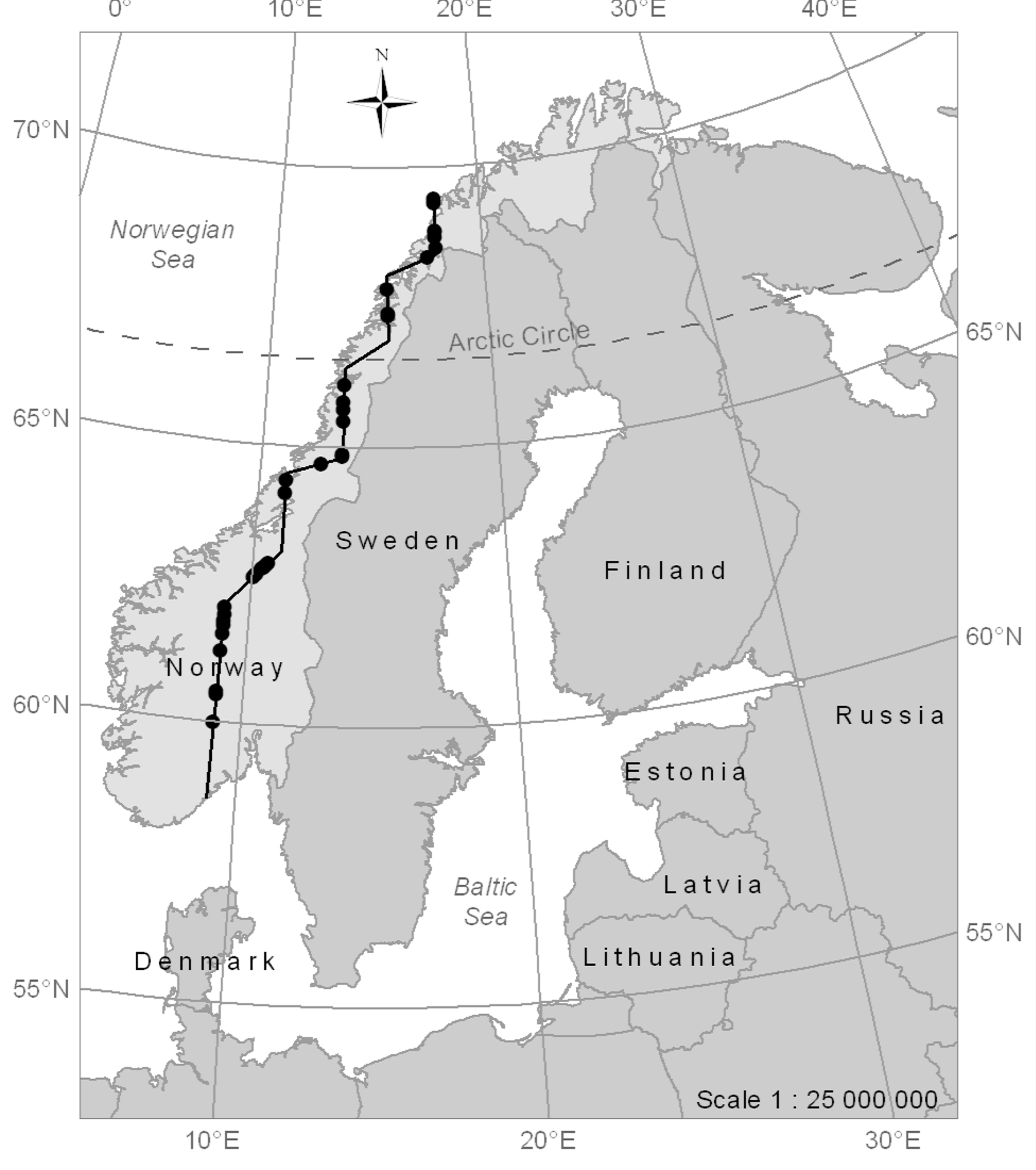
The study was conducted along a 1500 km long and approximately 180 m wide north-south transect that encompasses hundreds of mountain forest and alpine elevation gradients. The transect stretches from close to Tromsø in the northern part of Norway (69°32′25″N, 17°46′0″E) to close to Tvedestrand in the southern part of the country (58°36′6″N, 9°1′50″E) (Figure 1). It covers sample plots in the transition between the mountain forest and the alpine zone, where the terrain is often characterised by rounded forms, but also occurrences of hummocks, rocks and boulders, and steep slopes. The prevalent tree species were Norway spruce (Picea abies (L.) Karst.), Scots pine (Pinus sylvestris L.), and mountain birch (Betula pubescens ssp czerepanovii).
2.2. Field Data
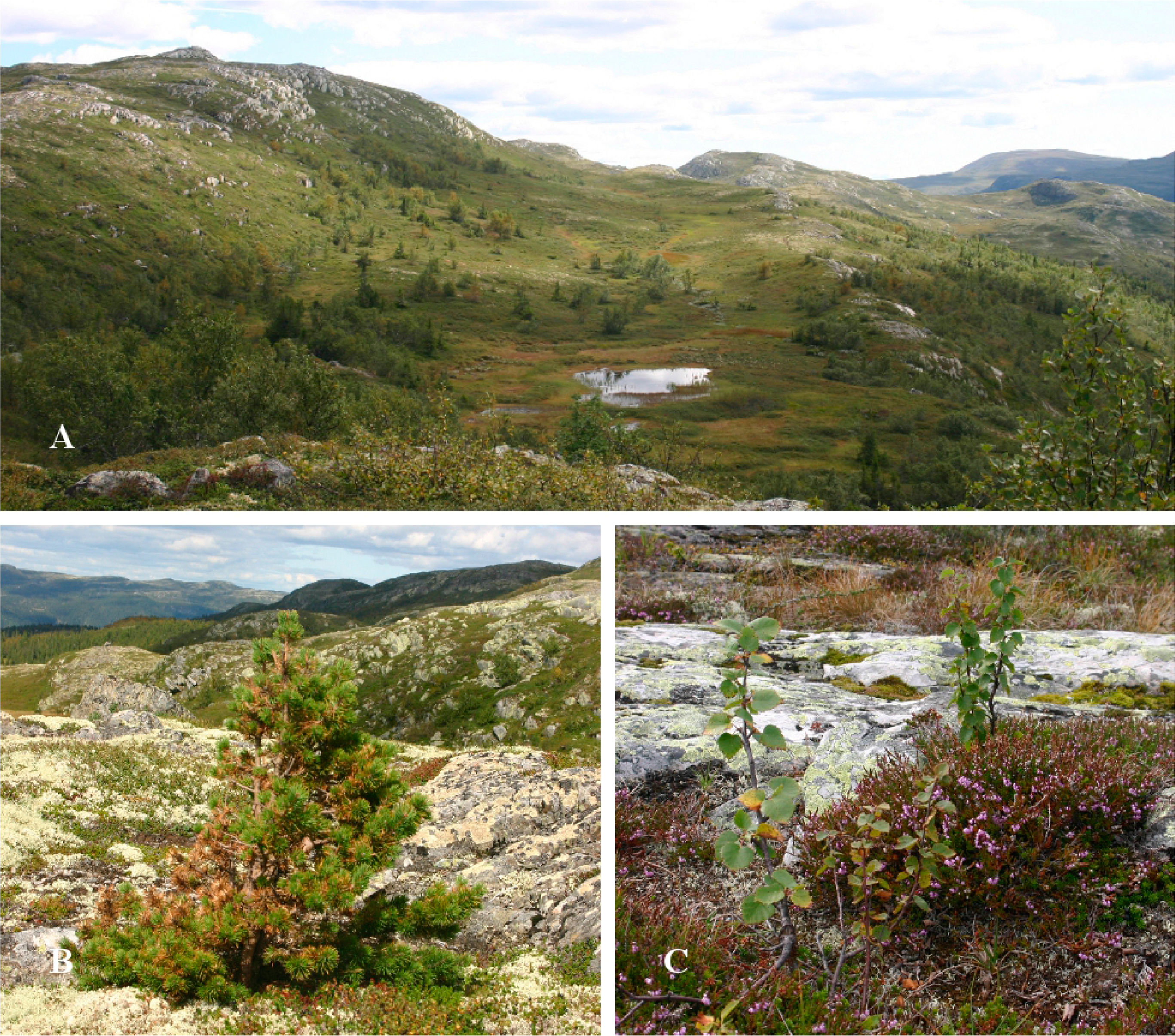
The field work was carried out in summer 2008 to provide in situ tree data from 35 different field sites allocated along the transect (Figure 2A). At each field site, two to four sample plots with a radius of 25 m were laid out to cover the range of the forest-tundra ecotone. The width of the forest-tundra ecotone varies for different locations and therewith the number of sample plots was adapted visually according to the altitudinal range of the ecotone at the specific site. To avoid overlap, sample plots were established along the transect with an interdistance of 50 m within field sites. In total, 111 sample plots were laid out at the 35 sites.
For the precise navigation and positioning, real-time kinematic differential Global Navigation Satellite Systems (dGNSS) was used. Two Topcon Legacy E+ 40-channel dual-frequency receivers observing pseudo range and carrier phase of up to 20 GPS and GLONASS satellites were used as base and rover receivers. A base station was established at the closest suitable reference point of the Norwegian Mapping Authority for each field site. The expected accuracy of the reference points was 3 cm, whereas the expected horizontal accuracy of the field recordings relative to the base station was about 2 cm. Thus, the expected accuracy of the sample plots centre points was 3–4 cm.
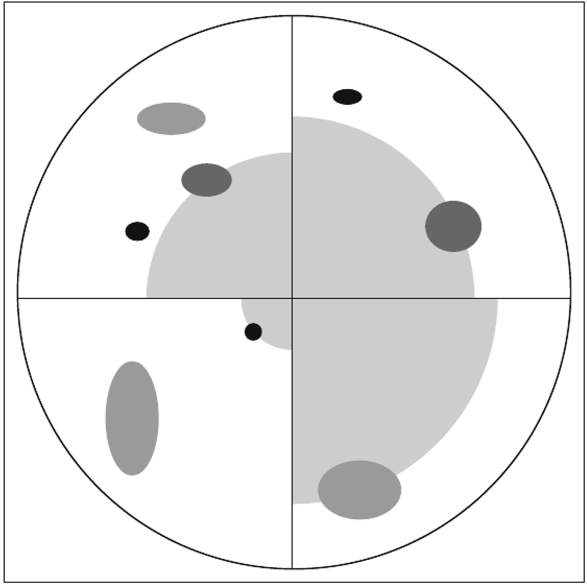
Individual sample trees (Figure 2B,C) were selected for measurement within each plot. Three mutually exclusive tree height classes were used for the tree selection: (1) lower than 1 m, (2) between 1 m and 2 m, and (3) taller than 2 m. A modified version of the point-centred quarter sampling method (PCQ) [26,27] was used for selection (Figure 3). In the process, each sample plot was divided into four quadrants defined by the cardinal directions from the sample plot centre using a Suunto compass. In each quadrant the trees that were closest to the sample plot centre in the respective tree height classes were sampled independent of tree species and with a maximum search distance of 25 m. In cases of doubt, the maximum search limit and the closest tree were determined using a surveyor’s tape measure.
Several tree parameters were recorded individually for each sample tree. Stem diameter was callipered at root collar and tree height was measured with a steel tape measure or a Vertex III hypsometer for tall trees. Crown diameters were measured in the cardinal directions using a steel tape measure and tree species was determined. For each sample tree, the precise position was captured using dGNSS.
In this study, a total of 744 trees were measured. However, ten trees were regarded as invalid for the analyses because of their tree crown areas being completely overlapped by tree crown areas of taller trees. These ten trees were discarded from the dataset, which resulted in a total number of 734, i.e., 614 mountain birch, 67 Norway spruce, and 53 Scots pine, included in this study. Tree heights ranged between 0.02 m and 7.80 m and about 46% of the trees were less than 1 m. Tree crown areas were computed as the ellipse defined by the crown diameters as major and minor axes and ranged from 0.001 to 19.54 m2. A summary of the tree parameters is given in Table 1. Thieme et al. [22] provides more details for the dataset.
2.3. Laser Data
Airborne laser scanner data were collected in two separate acquisitions because of the large geographical extent of the study area and difficult weather conditions. The first acquisition was carried out in southern and central Norway on 23 and 24 July 2006 using an Optech ALTM 3100C laser scanning system. This type of instrument has demonstrated that it is capable of producing mapping data with relative accuracies on the sub-decimeter level [28]. The second acquisition in northern Norway was conducted on 1 July 2007 with a Gemini upgraded version of the Optech ALTM 3100C laser scanner system, denoted as ALTM Gemini. An overlap zone in the county of Nordland (65°53′N 13°27′E) was scanned with both systems to provide approximately 80 km ALS data for comparison of the two systems. Thieme et al. [22] compared the data acquired by the two sensors and for individual trees located in the overlap zone and no significant difference in maximum tree height could be found. A Piper PA-31 Navajo aircraft carried both laser scanning systems at an average flying altitude of 800 m a.g.l. with a flight speed of approximately 75 ms−1. The scan frequency was 70 Hz, maximum half scan angle was 7°, and the average footprint diameter was estimated to 20 cm in both acquisitions. Pulse repetition frequency (PRF) was 100 kHz for the ALTM 3100C laser scanner system resulting in a mean pulse density of 6.8 m−2. To obtain laser point clouds as similar as possible for the two acquisitions, the PRF was set to 125 kHz for the ALTM Gemini system, as suggested by a test flight in May 2007 conducted in another area. This resulted in a mean pulse density of 8.5 m−2 for the acquisition in northern Norway in 2007. To keep the flying altitude above the terrain and hence the pulse density as constant as possible, the 1500 km long transect was split into 147 individual flight lines.
Pre-processing of the laser data was accomplished by a contractor (Blom Geomatics Norway), computing planimetric coordinates (x and y) and ellipsoidal height values for all laser echoes. Laser echoes labelled “last-of-many” and “single”, hereafter denoted as LAST, were used for the derivation of the terrain model. Ground echoes were classified from the planimetric coordinates and the corresponding height values of the LAST echoes using the progressive triangulated irregular network (TIN) densification algorithm [29] of the TerraScan software [30]. An iteration distance of 1.0 m and an iteration angle of 9° were used. Furthermore, laser echoes labelled as “first-of-many” and “single”, hereafter denoted as FIRST, were used for the analysis in the current study. For this purpose, the FIRST echoes were projected onto the TIN surface and corresponding terrain height on these locations was interpolated. The height differences between the FIRST echo heights and the corresponding interpolated terrain height values were computed and stored. For the present analysis, only FIRST echoes with height values greater than zero were used because this criterion represents the sole indicator for the presence of objects on the terrain surface.
Both the ALTM 3100C and the ALTM Gemini instrument record up to four echoes per laser pulse with a minimum vertical distance of 2.1 m between two subsequent echoes of an individual laser pulse for the ALTM 3100C. Because of the pulse width influencing the vertical resolution, the minimum vertical distance is assumed to be larger for the ALTM Gemini (cf. Baltsavias [31]). However, in combination with low vegetation, this instrument property involves that very few pulses have more than a single echo. Therefore, the LAST and FIRST datasets will be identical for many of the sample plots.
3. Methods
3.1. Background
The background of the present study was the development of an algorithm for automatic detection of small single trees in the forest-tundra ecotone using high-density ALS data based on an unsupervised classification approach classifying tree and nontree raster cells. In general, unsupervised classification methods involve cluster analysis where elements are aggregated to homogeneous classes without any reference or training data. Based on statistical parameters, each element is assigned to a specific class without any information on the thematic content or affiliation of the respective element.
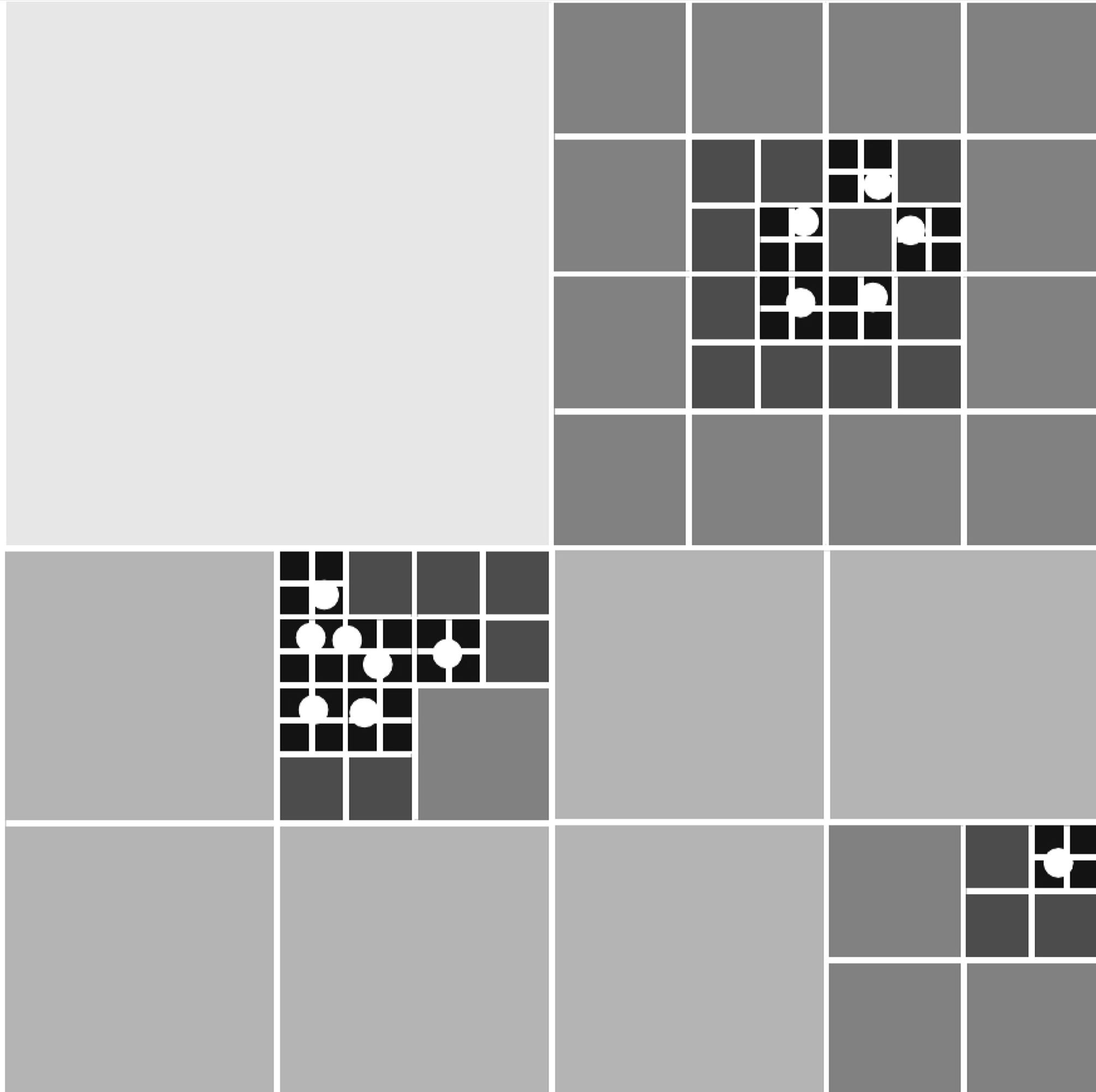
For this purpose, a concept for a raster-based algorithm was developed employing grids with decreasing raster cell sizes as provided by a region quadtree approach (Figure 4). In general, region quadtrees are used as a systematic procedure to display homogeneous parts of an image [32]. Based on a chosen criterion, an “image array is successively subdivided into quadrant, subquadrants, etc. until homogeneous blocks are obtained” [32] and a regular decomposition of the image is obtained.
Here, the main idea was to overlay the ALS data with the different grids in order to receive a binary raster where raster cells containing at least one laser echo are assigned the value 1 and empty raster cells the value 0. In an algorithmic context, the classification would start using a grid with a relatively large raster cell size that would be intersected with the ALS data and in case of a positive response, i.e., the presence of at least one laser echo, the raster cell would be quartered and again overlaid with the laser data. This procedure would be repeated until the raster cell is assigned the value 0 or until the minimum cell size is reached. Finally, using the raster with the minimum raster cell size, all cells with value 1 would be aggregated to tree clusters using a commonly adopted clustering analysis (see e.g., [33]), however, the clustering is not a part of the current study. Figure 4 illustrates the entire process.
In this study, the focus was on finding suitable initial values starting the process and excluding large treeless areas, as well as determining the optimal raster cell size that can further be used to aggregate the raster cells to trees. The implementation of the algorithm was not prioritised in this stage.
3.2. Computations
In order to assess the accuracy of an unsupervised classification for automatic detection of small single trees in the forest-tundra ecotone, tree and nontree polygons had to be computed. For this purpose, the field-measured crown diameters were used to estimate elliptical tree crown polygons. The contractor reported a horizontal positioning error of the laser data of up to 0.5 m. Therefore, trees with a crown diameter value less than 1.0 m in at least one cardinal direction were assigned a tree crown polygon with a constant radius of 0.5 m emanating from the centre of the tree, i.e., the measured location.
Furthermore, nontree polygons were generated utilising the basic properties of the PCQ method resulting in full control of some of the areas without any trees. For each plot, the sampling design of the PCQ method led to a maximum of three sampled trees per quadrant. The tree closest to the respective plot centre was selected irrespective of tree height class in each of the four quadrants (Figure 3). Using the areas between the selected tree in a quadrant and the respective plot centres, nontree polygons were computed. In this process, the tree crown polygons of the selected trees were erased from the nontree polygons to obtain full control over the treeless areas.
3.3. Analysis
To assess the capability of an unsupervised classification to distinguish between tree and nontree raster cells, parts of the raster-based algorithm concerning the utilisation of grids with different raster cell sizes were tested. For this purpose, raster map layers were rectified to the plots and different raster cell sizes were adapted to the size of the sample plots starting with the radius of the sample plot as the initial raster cell side length. Raster cell side lengths ranged from 25 m to 39 cm, which resulted in raster cell sizes of 625 m2 and down to 0.153 m2. Table 2 gives an overview over the different raster cell sizes used in the current analysis. Furthermore, the suitability of different height thresholds for the laser echoes included to detect tree raster cells in an unsupervised classification approach was assessed: 0 cm, 10 cm, 20 cm, 30 cm, 40 cm, and 50 cm. Albeit different ALS-derived variables have been employed for the supervised classification of tree and nontree laser echoes, laser height represents the strongest indicator for the presence of trees. Thus, only laser height was used in the current analysis to assess the capability of an unsupervised classification method for the classification of tree and nontree raster cells.
For all classifications, grids were computed with the seven different raster cell sizes. Each grid was overlaid with ALS data using the six different laser height thresholds. Raster cells containing at least one laser echo were assigned the value 1, and empty raster cells the value 0. These grids were subsequently overlaid with the tree crown polygons in order to assess the classification performance. Raster cells classified as 1 were evaluated as successful detection when covered by a tree crown polygon or a part of it regardless of the size of the overlap area. The classifications are described in Table 3. In the first classification (I), all tree crown polygons were included irrespective of their tree height. For the second classification (II), only tree crown polygons with a tree height equal to or higher than the laser height thresholds were used. Furthermore, results of studies conducted by Næsset and Nelson [20] and Thieme et al. [22] suggested that when trees reach a height taller than 1 m they have a large potential for successful detection by an unsupervised raster-based classification, given a high laser point density. Therefore, a third classification (III) was assessed using only tree crown polygons with tree heights exceeding 1 m. Previous studies on the detection of small individual trees reported an underestimation of laser-derived tree heights compared to the corresponding tree heights measured in the field [20,22,23]. To investigate a potential effect of the underestimation of the laser-derived tree heights, classifications for the laser height thresholds of 20 cm and 30 cm were evaluated for tree crown polygons with field-measured tree heights larger than the respective thresholds. For the present dataset, Thieme et al. [22] reported mean underestimations of 20 cm for mountain birch, 29 cm for Norway spruce, and 47 cm for Scots pine, respectively. Because of the unbalanced tree species composition in the dataset, classifications were evaluated for tree crown polygons with tree heights of 30 cm, 40 cm and 50 cm for the laser height threshold of 20 cm (classification IV), and 40 cm and 50 cm for the laser height thresholds 30 cm (classification V). Commission errors were investigated by the intersection of the different grids with the nontree polygons.
To test if the mean detection success rates were statistically different when varying the ALS threshold and tree height restrictions, a simulation procedure was used. We selected at random, with replacement, from the pairwise observed and classified tree/nontree raster cell observations for each of the different cell sizes. The selection was continued until the random sample matched the size of the observed data, and this was repeated 100 times. The differences in detection success rate between all alternatives were calculated each time. Pairwise t-tests were applied to test if differences were significantly different from zero. The analysis was carried out for classification I (20 cm and 30 cm ALS thresholds) and classification II (20 cm and 30 cm ALS thresholds) to limit the output. However, if significant differences are obtained between adjacent ALS thresholds and tree height classes, it can be assumed that differences are significant also between more distant classes.
4. Results and Discussion
4.1. Raster Cell Sizes
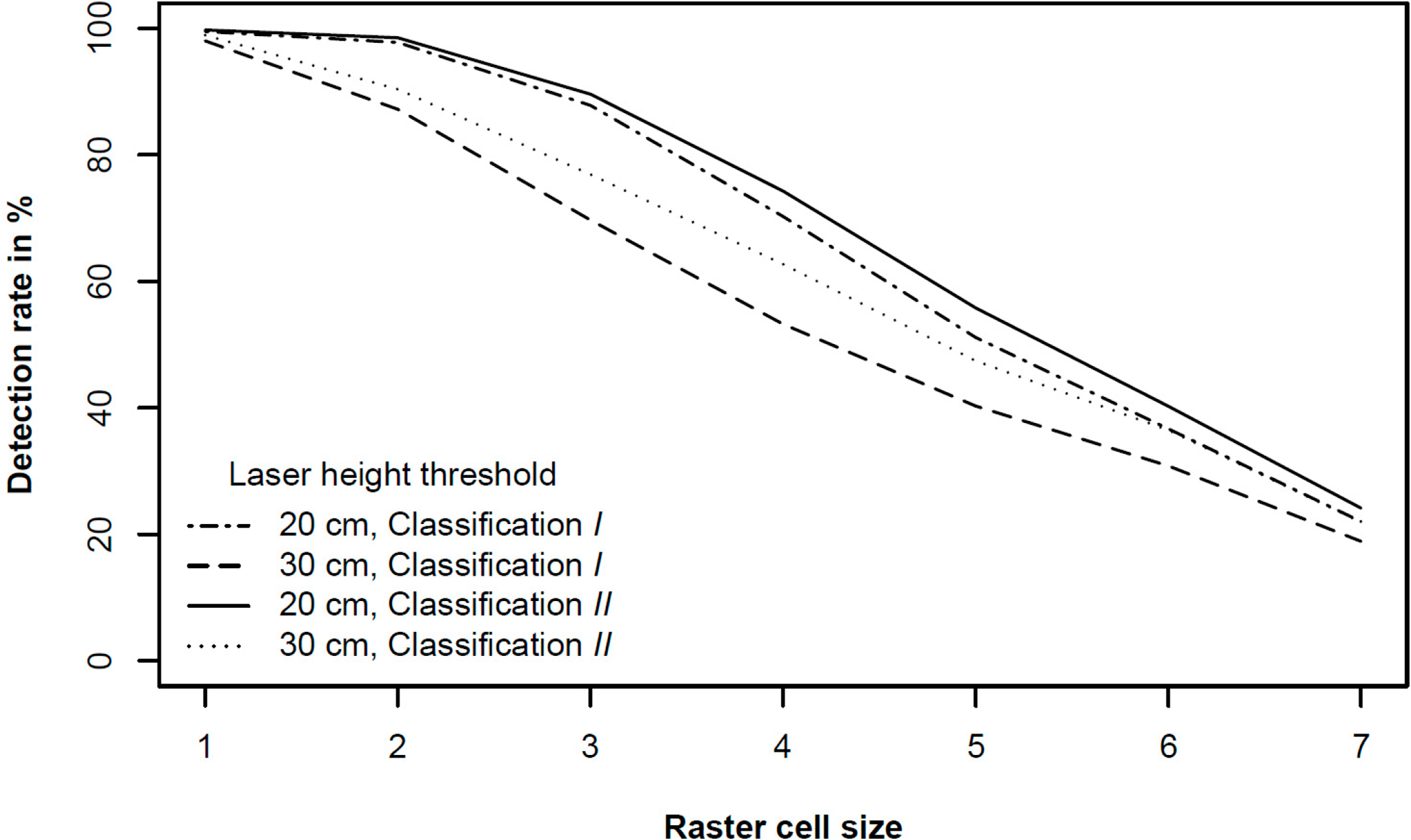
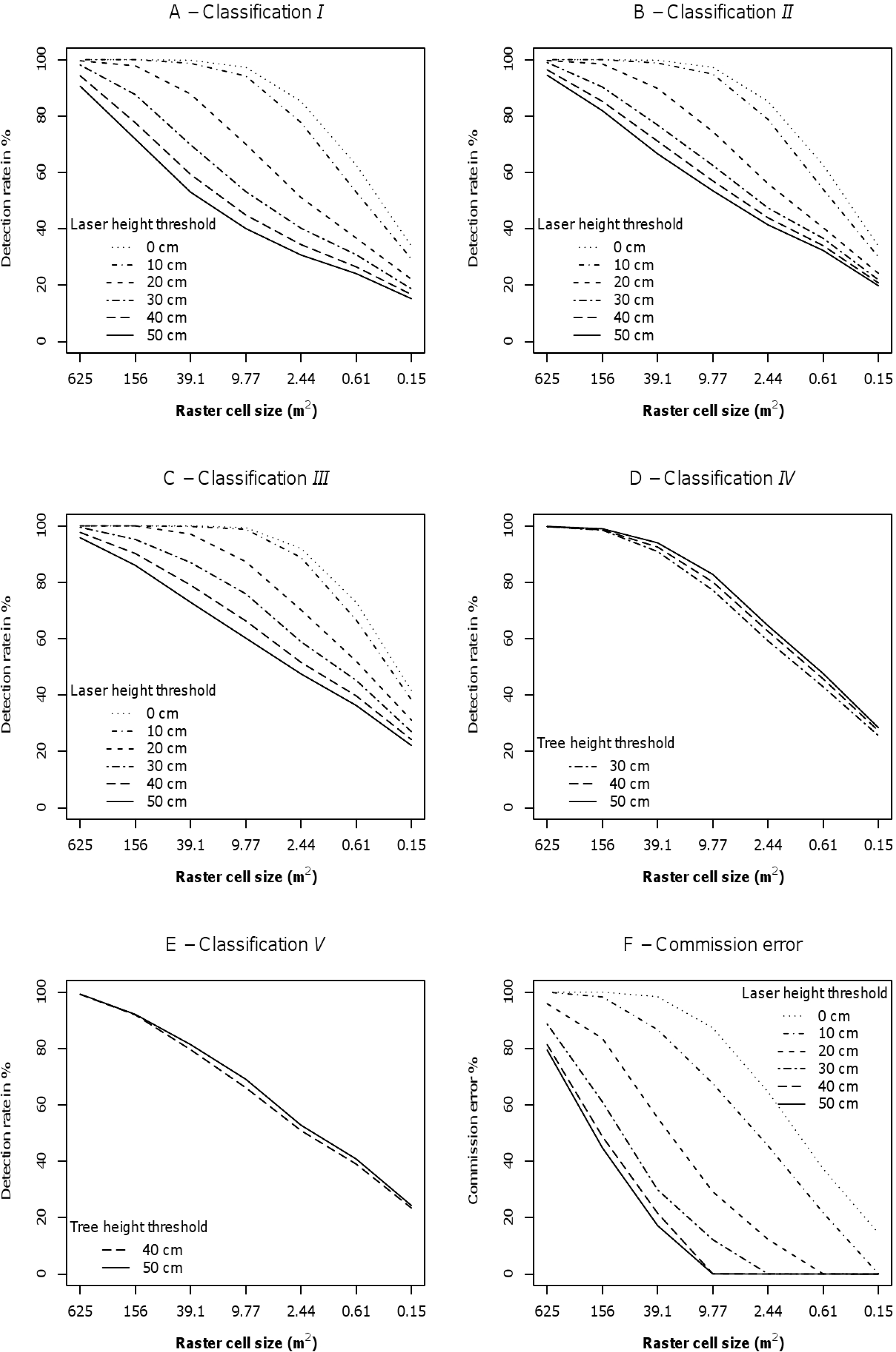
Generally, the detection success rates decreased with decreasing raster grid cell size (Figure 5). Starting with an initial value of 625 m2, which corresponds to approximately a quarter of the sample plot size in this study, the three largest raster cell sizes 1 with 625 m2, 2 with 156 m2, and 3 with 39.1 m2 (Table 2) were well suited for the exclusion of areas without any trees in all classifications. However, these raster cell sizes were too large for reliable tree raster cell detection since the description of the positioning of the small trees is very imprecise using such large raster cell sizes.
Raster cell size 6 with 0.61 m2 (Table 2), that is approximately half the size of the mean tree crown area, was identified as the optimal raster cell size in terms of a small raster cell size providing a relatively precise description of the positioning of the small trees and still satisfying detection success rates. In all classifications for raster cell size 6, 24.1 to 72.9% of the tree raster cells were classified correctly depending on the laser height threshold (Figures 5A–E). For raster cell size 7 with 0.15 m2 (Table 2), however, a substantial decrease in the success rate of the tree raster cell detection was found (Figures 5A–E). Therewith, raster cell sizes that are considerably smaller than half of the mean tree crown area seem to be too small and hence inapplicable for the detection of tree raster cells.
4.2. Laser Height Thresholds
The rates of commission errors ranged from zero to 100% (Figure 5F). The commission errors decreased with increasing laser height threshold. For the classifications I, II, and III, the laser height thresholds of 20 cm and 30 cm represented turning points concerning the rates of commission error which was emphasised by a substantial decrease of nontree raster cells classified as tree raster cells for the respective raster cell sizes 3 to 6 (Figure 5F). This distinct decrease in commission errors for the two laser height thresholds suggested a diminution in laser data noise in the range of 20 cm to 30 cm and supported an assumption of such an upper limit as observed during data processing. Furthermore, ALS thresholds of 20–30 cm correspond to the uncertainty of the terrain model [34–36]. Further, a study conducted by Nyström et al. [37] in northern Sweden using ALS data to measure tree height of newly established individual trees (0.3–2.6 m) in former pasture land merely included trees with heights exceeding 30 cm. There, the rate for successful tree detection for trees shorter than 1 m was considerably higher than in the present study. Even if the conditions were different, this might give an indication of laser data noise being reduced around 30 cm. For higher laser height thresholds, a decrease in the number of nontree raster cells classified as tree raster cells was almost non-existent for the raster cell sizes mentioned earlier (Figure 5F).
4.3. Differences between Alternative Classifications
Figure 6 shows that the mean detection success rate for the selected classifications was highest for classification II with ALS threshold- and tree height restriction of 20 cm irrespective of raster cell size. Then followed by classification I (20 cm), classification II (30 cm), and classification I (30 cm). The pairwise t-test revealed that all the simulated mean detection success rates were significantly different (p < 0.05) with two exceptions. For the two smallest raster cell sizes, the mean detection success rate for classification I (20 cm) could not be distinguished from that of classification II (30 cm). This suggests that both ALS threshold and tree height restriction significantly matters for the detection success rate, but that the raster grid cell size should be kept at least equal to our cell size 6 (0.78 m2). As mentioned before, in this particular study the positioning error of the laser data could be up to 0.5 m, and this will affect the optimal raster grid cell size.
4.4. Classification for Raster Cell Size 6
Because of its identification as the optimal raster cell size the following subsection presenting and discussing the results of the different classifications refers to raster cell size 6. For classification I where the accuracy of the classification was assessed using all field-measured tree data without any restriction of the tree height to the laser height thresholds, at least 24.1% and up to 62.6% of the tree raster cells were found depending on the laser height threshold (Figure 5A). By restricting the tree heights to the laser height threshold for the echoes included in the classification (classification II), the accuracy of the classification ranged between 32.3% and 62.6% depending on the laser height threshold (Figure 5B). For tree heights exceeding a height of 1 m (classification III), the rates of successful detection ranged between 36.3% and 72.9% for the different thresholds (Figure 5C).
Results from classification III where the accuracy was assessed using trees with tree heights larger than 1 m revealed slightly lower detection rates than found by previous studies on small individual tree detection in the forest-tundra ecotone [20,22,23]. However, in this raster-based approach, the detection rates apply to the tree raster cells and not the individual trees themselves, which may have an influence on the detection rates in the present study.
For the classifications with laser height thresholds of 20 cm (IV) and 30 cm (V), success rates for the detection of tree raster cells ranged between 42.9% and 47.6% (Figure 5D), and 39.0% and 40.8% (Figure 5E), respectively. Both classifications revealed higher success rates for higher tree height thresholds. However, the differences between the success rates for the different tree height thresholds were low for classification IV and almost equal to zero for classification V (Figure 5D,E). These results revealed an increase in successful detection of tree pixels by increasing the height of trees included in the classification. This behaviour reflects the influence of a potential underestimation of real tree height using ALS data as demonstrated by Næsset and Nelson [20], Thieme et al. [22], and Næsset [23].
4.5. Suitability for Monitoring Purposes
The results from the different classifications revealed that the parameters for raster cell sizes, laser height threshold of the echoes included, as well as a potential lower tree height limit, have to be chosen carefully ensuring a justifiable trade-off between detection success rates and commission errors. For monitoring purposes also additional challenges represented by the usage of different sensors and acquisition settings over time [23] have to be met.
The time lag of the different data acquisitions is a shortcoming of the dataset used in the current study. As mentioned earlier, ALS data were collected in July 2006 and June 2007, whereas the field work was carried out in summer 2008. Concerning the ALS data in 2007, the acquisition was conducted before the growing season in order to avoid biased measurements compared to the data collection in 2006.
The field work was carried out during one growing season after the ALS data. This might mean that some trees close to the limits of the tree height classes actually are assigned to another tree height class in the field data as in the ALS dataset. A height correction was not taken into account, because ALS already underestimates the real tree height. Furthermore, small trees can grow tens of centimetres at productive sites during a year, however, in a mountain forest environment the height of such small trees also could remain stable. Since these circumstances are hard to model, no data adjustment was conducted. A better match in time between the acquisitions might have improved the results.
Varying laser point densities caused by the usage of different instruments have to be tested for their comparability. In general, the probability of a tree for being hit by at least one laser pulse is a function of the laser point density. Low point densities may therewith not be capable to detect trees with sizes that are typical in the forest-tundra ecotone. Næsset and Nelson [20], as well as Thieme et al. [22] reported that almost all trees exceeding 1 m in height were hit by at least one laser pulse using high-density ALS data with point densities ranging from 6.8 to 8.5 m−2. However, in this dataset high point densities involved a relatively large proportion of data noise for laser echoes with heights lower than 20–30 cm as revealed by the sudden decrease of commission errors for these thresholds in the present analysis. Nyström et al. [38] introduced a procedure to compensate for unevenly distributed laser points and concluded that ALS has strong potential as a data source to map mountain birch biomass in the forest-tundra ecotone, even when using sparse point density ALS data. However, in the forest-tundra ecotone, the smallest trees and other typical vegetation such as shrubs are often equal in height, which limits their distinguishability considerably. Thus, severe commission errors may occur using an unsupervised classification technique only employing laser height values.
A shortcoming of the method might be that other objects than trees could be detected. However, in a monitoring context other objects would remain stable in height whereas trees are expected to grow over time. Furthermore, data acquisitions with a sufficient time span are essential to detect regeneration and mortality of small individual trees. Experimental changes of mountain birch tree cover in the forest-tundra ecotone have been successfully classified using histogram matching based on ALS data [39]. Tree height growth is detectable over relatively short time spans as 2 to 5 years both using high- and low-density ALS data [40,41]. However, for small individual trees located in the forest-tundra ecotone, tree height growth is strongly depending on local climatic and topographic conditions. Based on an assumed height growth of 1 to 10 cm per year for small trees, longer time spans may be required for such a raster-based automatic detection algorithm, especially with regard to tree establishment.
5. Conclusion
To conclude, the present study demonstrated the potential of an unsupervised classification approach for the automatic detection of small individual trees in the forest-tundra ecotone based on high-density airborne laser scanning data. The field and laser data comprise a unique study area along a 1500 km long transect covering numerous of mountain forest and alpine elevation gradients. By employing different raster cell sizes, suitable initial values for the exclusion of large areas without any laser echoes reflected from trees could be recognised providing an efficient tool for data processing. Furthermore, a lower limit for raster cell sizes was determined providing a relatively precise description of the positioning of the small trees and still ensuring a satisfying rate of successfully detected tree raster cells.
With regard to the laser height thresholds for the laser echoes included in the respective classifications, the thresholds of 20 cm and 30 cm turned out to be the turning points where the rate of nontree raster cells classified as tree raster cells decreased substantially, accompanied by a still satisfying rate of successfully detected tree raster cells. Further research should be devoted to clustering the raster cells into tree clusters.
Airborne laser scanning has already been adopted for NFI and monitoring programmes, e.g., the Land Use and Carbon Analysis System in New Zealand [42]. In context of a national monitoring program covering such vast areas as the forest-tundra ecotone in Norway, the present study provides an unsupervised classification technique on a large scale that is useful to detect regeneration and mortality of small individual trees. For this purpose, it is advisable to identify a laser point density that is high enough to detect the small objects of interest. Then, provided a sufficient time span and an adequate selection of raster cell sizes and laser height threshold of the echoes included, successful detection of small individual trees with satisfying detection rates is achievable. The raster grid cells may further build the basis for map products presenting variation of tree presence over time.
Acknowledgments
This research has been funded by the Research Council of Norway (project #184636/S30). We wish to thank Blom Geomatics AS, Norway, for collection and processing of the airborne laser scanner data. Thanks also appertain to Mr. Vegard Lien at the Norwegian University of Life Sciences, who was responsible for the fieldwork. Finally, we would like to thank the five anonymous reviewers for valuable and constructive comments and suggestions.
Author Contributions
Nadja Stumberg has been the main author of the manuscript, carried out calculations and analyses in the study, conducted parts of the field work and revised the manuscript. Ole Martin Bollandsås has planned and prepared the field data, carried out error analysis and revised parts of the manuscript. Terje Gobakken has prepared the remote sensing data, carried out error analysis, supervised parts of the study and has revised the manuscript. Erik Næsset has planned and prepared the remote sensing data, detailed the field sampling design, supervised the study and revised parts of the manuscript.
Conflicts of Interest
The authors declare no conflict of interest.
References and Notes
- Holtmeier, F.-K.; Broll, G. Sensitivity and response of northern hemisphere altitudinal and polar treelines to environmental change at landscape and local scales. Global Ecol. Biogeogr 2005, 14, 395–410. [Google Scholar]
- Callaghan, T.V.; Werkman, B.R.; Crawford, R.M.M. The tundra-taiga interface and its dynamics: Concepts and applications. Ambio 2002, 6–14. [Google Scholar]
- Clements, F.E. Research Methods in Ecology; University Publishing Company: Lincoln, NL, USA, 1905. [Google Scholar]
- Harper, K.A.; Danby, R.K.; De Fields, D.L.; Lewis, K.P.; Trant, A.J.; Starzomski, B.M.; Savidge, R.; Hermanutz, L. Tree spatial pattern within the forest–tundra ecotone: A comparison of sites across canada. Can. J. For. Res 2011, 41, 479–489. [Google Scholar]
- ACIA. Impacts of a Warming Arctic: Arctic Climate Impact Assessment; Cambridge University Press: Cambridge, UK, 2004. [Google Scholar]
- Batllori, E.; Gutiérrez, E. Regional tree line dynamics in response to global change in the pyrenees. J. Ecol 2008, 96, 1275–1288. [Google Scholar]
- Danby, R.K.; Hik, D.S. Variability, contingency and rapid change in recent Subarctic Alpine tree line dynamics. J. Ecol 2007, 95, 352–363. [Google Scholar]
- Kullman, L. Rapid recent range-margin rise of tree and shrub species in the Swedish Scandes. J. Ecol 2002, 90, 68–77. [Google Scholar]
- Kullman, L.; Öberg, L. Post-Little Ice Age tree line rise and climate warming in the Swedish Scandes: A landscape ecological perspective. J. Ecol 2009, 97, 415–429. [Google Scholar]
- Aune, S.; Hofgaard, A.; Söderström, L. Contrasting climate- and land-use-driven tree encroachment patterns of subarctic tundra in northern Norway and the Kola Peninsula. Can. J. For. Res 2011, 41, 437–449. [Google Scholar]
- Sturm, M.; Schimel, J.; Michaelson, G.; Welker, J.M.; Oberbauer, S.F.; Liston, G.E.; Fahnestock, J.; Romanovsky, V.E. Winter biological processes could help convert Arctic tundra to shrubland. BioScience 2005, 55, 17–26. [Google Scholar]
- Cairns, D.M.; Moen, J. Herbivory influences tree lines. J. Ecol 2004, 92, 1019–1024. [Google Scholar]
- Hofgaard, A.; Løkken, J.O.; Dalen, L.; Hytteborn, H. Comparing warming and grazing effects on birch growth in an alpine environment—A 10-year experiment. Plant Ecol. Divers 2010, 3, 19–27. [Google Scholar]
- Post, E.; Pedersen, C. Opposing plant community responses to warming with and without herbivores. Proc. Natl. Acad. Sci. USA 2008, 105, 12353–12358. [Google Scholar]
- Olofsson, J.; Oksanen, L.; Callaghan, T.; Hulme, P.E.; Oksanen, T.; Suominen, O. Herbivores inhibit climate-driven shrub expansion on the tundra. Glob. Chang. Biol 2009, 15, 2681–2693. [Google Scholar]
- UNFCCC. Kyoto Protocol Reference Manual on Accounting of Emissions and Assigned Amount; United Nations Framework Convention on Climate Change: Bonn, Germany, 2008. [Google Scholar]
- Hyyppa, J.; Kelle, O.; Lehikoinen, M.; Inkinen, M. A segmentation-based method to retrieve stem volume estimates from 3-D tree height models produced by laser scanners. IEEE Trans. Geosci. Remote Sens 2001, 39, 969–975. [Google Scholar]
- Persson, Å.; Holmgren, J.; Söderman, U. Detecting and measuring individual trees using an airborne laser scanner. Photogramm. Eng. Remote Sensing 2002, 68, 925–932. [Google Scholar]
- Solberg, S.; Næsset, E.; Bollandsås, O.M. Single tree segmentation using airborne laser scanner data in a structurally heterogeneous spruce forest. Photogramm. Eng. Remote Sensing 2006, 72, 1369–1378. [Google Scholar]
- Næsset, E.; Nelson, R. Using airborne laser scanning to monitor tree migration in the boreal-alpine transition zone. Remote Sens. Environ 2007, 110, 357–369. [Google Scholar]
- Rees, W.G. Characterisation of arctic treelines by lidar and multispectral imagery. Polar Rec 2007, 43, 345–352. [Google Scholar]
- Thieme, N.; Bollandsås, O.M.; Gobakken, T.; Næsset, E. Detection of small single trees in the forest-tundra ecotone using height values from airborne laser scanning. Can. J. Remote Sens 2011, 37, 264–274. [Google Scholar]
- Næsset, E. Influence of terrain model smoothing and flight and sensor configurations on detection of small pioneer trees in the boreal–alpine transition zone utilizing height metrics derived from airborne scanning lasers. Remote Sens. Environ 2009, 113, 2210–2223. [Google Scholar]
- Stumberg, N.; Ørka, H.O.; Bollandsås, O.M.; Gobakken, T.; Næsset, E. Classifying tree and nontree echoes from airborne laser scanning in the forest–tundra ecotone. Can. J. Remote Sens 2012, 38, 655–666. [Google Scholar]
- Stumberg, N.; Hauglin, M.; Bollandsås, O.M.; Gobakken, T.; Erik, N. Improving classification of airborne laser scanning echoes in the forest-tundra ecotone using geostatistical and statistical measures. Remote Sens 2014, 6, 4582–4599. [Google Scholar]
- Warde, W.; Petranka, J.W. A correction factor table for missing point-center quarter data. Ecology 1981, 62, 491–494. [Google Scholar]
- Cottam, G.; Curtis, J.T. The use of distance measures in phytosociological sampling. Ecology 1956, 37, 451–460. [Google Scholar]
- Ussyshkin, R.V.; Smith, B. Performance evaluation of Optech’s ALTM 3100EA: Instrument specifications and accuracy of lidar data. Int. Arch. Photogramm. Remote Sens. Spat. Inf. Sci 2006, 34. Part 1.. [Google Scholar]
- Axelsson, P. Dem generation from laser scanner data using adaptive tin models. Int. Arch. Photogramm. Remote Sens. Spat. Inf. Sci 2000, 33(B4), 111–118. [Google Scholar]
- Terrasolid. Terrascan User’s Guide. Available online: www.terrasolid.fi (accessed on 26 September 2011).
- Baltsavias, E.P. Airborne laser scanning: Basic relations and formulas. ISPRS J. Photogramm. Remote Sens 1999, 54, 199–214. [Google Scholar]
- Samet, H. The quadtree and related hierarchical data structures. ACM Comput. Surv 1984, 16, 187–260. [Google Scholar]
- Jain, A.K.; Murty, M.N.; Flynn, P.J. Data clustering: A review. ACM Comput. Surv 1999, 31, 264–323. [Google Scholar]
- Hodgson, M.E.; Bresnahan, P. Accuracy of airborne lidar-derived elevation: Empirical assessment and error budget. Photogramm. Eng. Remote Sensing 2004, 70, 331–339. [Google Scholar]
- Kraus, K.; Pfeifer, N. Determination of terrain models in wooded areas with airborne laser scanner data. ISPRS J. Photogramm. Remote Sens 1998, 53, 193–203. [Google Scholar]
- Peng, M.-H.; Shih, T.-Y. Error assessment in two lidar-derived tin datasets. Photogramm. Eng. Remote Sensing 2006, 72, 933–947. [Google Scholar]
- Nyström, M. Mapping and Monitoring of Vegetation Using Airborne Laser Scanning. Ph.D. Thesis, Dept. of Forest Resource Management. Swedish University of Agricultural Sciences, Umeå, Sweden, 2014; p. 72. [Google Scholar]
- Nyström, M.; Holmgren, J.; Olsson, H. Prediction of tree biomass in the forest–tundra ecotone using airborne laser scanning. Remote Sens. Environ 2012, 123, 271–279. [Google Scholar]
- Nyström, M.; Holmgren, J.; Olsson, H. Change detection of mountain birch using multi-temporal ALS point clouds. Remote Sens. Lett 2012, 4, 190–199. [Google Scholar]
- Yu, X.; Hyyppä, J.; Kukko, A.; Maltamo, M.; Kaartinen, H. Change detection techniques for canopy height growth measurements using airborne laser scanner data. Photogramm. Eng. Remote Sensing 2006, 72, 1339–1348. [Google Scholar]
- Næsset, E.; Gobakken, T. Estimating forest growth using canopy metrics derived from airborne laser scanner data. Remote Sens. Environ 2005, 96, 453–465. [Google Scholar]
- Beets, P.N.; Brandon, A.; Fraser, B.V.; Goulding, C.J.; Lane, P.M.; Stephens, P.R. National forest inventories: New Zealand. In National Forest Inventories—Pathways for Common Reporting; Tomppo, E., Gschwantner, T., Lawrence, M., McRoberts, R.E., Eds.; Springer: Berlin/Heidelberg, Germany, 2010; pp. 391–410. [Google Scholar]


| Tree Species | Characteristics | N | Mean | Min. | Max. |
|---|---|---|---|---|---|
| Mountain birch | Height (m) | 614 | 1.27 | 0.02 | 7.80 |
| Diameter (cm) | 613 a | 3.65 | 0.10 | 34.00 | |
| Crown area (m2) | 614 | 0.91 | 0.001 | 19.54 | |
| Norway spruce | Height (m) | 67 | 1.67 | 0.07 | 7.00 |
| Diameter (cm) | 65 a | 6.54 | 0.20 | 19.10 | |
| Crown area (m2) | 67 | 1.45 | 0.006 | 5.69 | |
| Scots pine | Height (m) | 53 | 1.33 | 0.10 | 5.10 |
| Diameter (cm) | 53 | 5.00 | 0.30 | 18.90 | |
| Crown area (m2) | 53 | 0.81 | 0.002 | 7.28 |
Note:
aMissing diameter measurements due to field conditions.| Label for Cell Size | Number of Cells | Cell Side Length (m) | Cell Size (m2) |
|---|---|---|---|
| 1 | 4 | 25 | 625.000 |
| 2 | 16 | 12.5 | 156.250 |
| 3 | 64 | 6.25 | 39.063 |
| 4 | 256 | 3.125 | 9.766 |
| 5 | 1024 | 1.5625 | 2.441 |
| 6 | 4096 | 0.78125 | 0.610 |
| 7 | 16,384 | 0.390625 | 0.153 |
| Classification | Reference Data Included | ALS Data Included |
|---|---|---|
| I | All trees | Five thresholds: 10 cm, 20 cm, 30 cm, 40 cm, and 50 cm |
| II | Trees with heights equal to or higher than the respective laser height thresholds | Five thresholds: 10 cm, 20 cm, 30 cm, 40 cm, and 50 cm |
| III | Trees with heights exceeding 1 m | Five thresholds: 10 cm, 20 cm, 30 cm, 40 cm, and 50 cm |
| IV | Three thresholds: 30 cm, 40 cm, and 50 cm | Laser echoes with heights higher than 20 cm |
| V | Two thresholds: 40 cm and 50 cm | Laser echoes with heights higher than 30 cm |
© 2014 by the authors; licensee MDPI, Basel, Switzerland This article is an open access article distributed under the terms and conditions of the Creative Commons Attribution license (http://creativecommons.org/licenses/by/4.0/).
Share and Cite
Stumberg, N.; Bollandsås, O.M.; Gobakken, T.; Næsset, E. Automatic Detection of Small Single Trees in the Forest-Tundra Ecotone Using Airborne Laser Scanning. Remote Sens. 2014, 6, 10152-10170. https://doi.org/10.3390/rs61010152
Stumberg N, Bollandsås OM, Gobakken T, Næsset E. Automatic Detection of Small Single Trees in the Forest-Tundra Ecotone Using Airborne Laser Scanning. Remote Sensing. 2014; 6(10):10152-10170. https://doi.org/10.3390/rs61010152
Chicago/Turabian StyleStumberg, Nadja, Ole Martin Bollandsås, Terje Gobakken, and Erik Næsset. 2014. "Automatic Detection of Small Single Trees in the Forest-Tundra Ecotone Using Airborne Laser Scanning" Remote Sensing 6, no. 10: 10152-10170. https://doi.org/10.3390/rs61010152
APA StyleStumberg, N., Bollandsås, O. M., Gobakken, T., & Næsset, E. (2014). Automatic Detection of Small Single Trees in the Forest-Tundra Ecotone Using Airborne Laser Scanning. Remote Sensing, 6(10), 10152-10170. https://doi.org/10.3390/rs61010152