Abstract
Real-time estimation of crop progress stages is critical to the US agricultural economy and decision making. In this paper, a Hidden Markov Model (HMM) based method combining multisource features has been presented. The multisource features include mean Normalized Difference Vegetation Index (NDVI), fractal dimension, and Accumulated Growing Degree Days (AGDDs). In our case, these features are global variable, and measured in the state-level. Moreover, global feature in each Day of Year (DOY) would be impacted by multiple progress stages. Therefore, a mixture model is employed to model the observation probability distribution with all possible stage components. Then, a filtering based algorithm is utilized to estimate the proportion of each progress stage in the real-time. Experiments are conducted in the states of Iowa, Illinois and Nebraska in the USA, and our results are assessed and validated by the Crop Progress Reports (CPRs) of the National Agricultural Statistics Service (NASS). Finally, a quantitative comparison and analysis between our method and spectral pixel-wise based methods is presented. The results demonstrate the feasibility of the proposed method for the estimation of corn progress stages. The proposed method could be used as a supplementary tool in aid of field survey. Moreover, it also can be used to establish the progress stage estimation model for different types of crops.
1. Introduction
Crop phenological phases, which reflect the timing of recurring biological events, play an important role in US agricultural production, management, planning and decision-making. Real-time accurate estimation of crop progress stages is desired during growing season. The National Agricultural Statistics Service (NASS) of the United States Department of Agriculture (USDA) issues Crop Progress Reports (CPRs) [1] weekly during the growing season, listing primary progresses of selected crops in major producing states and Agricultural Statistics Districts (ASDs) through field survey. Despite its accuracy, only site-specific information in limited geographical extent can be provided. Especially, field survey is labor intensive and time-consuming. Therefore, it is very necessary to find a supplementary way for efficient, quantitative, and accurate estimating of crop progress stages.
Many algorithms and techniques have been developed to detect specific crop phenological stages, e.g., greenup, maturity, senescence and dormancy [2]. A comparison of several existing methods for analyzing remotely sensed time series is provided in Hird and McDermid [3], and Atkinson et al.[4]. Most of methods focus on the timing, duration and intensity of the growing season [5]. Growing degree days (thermal time or heat units) are generally applied for measuring different developmental events of crop [6,7]. Most of the process oriented crop growth models, e.g., WOrld FOod STudies (WOFOST) [8], Cropping Systems Simulator (CropSyst) [9], Decision Support System for Agrotechnology Transfer (DSSAT) series [10], Soil-Plant-Air-Water (SPAW) [11], and Soil-Water-Atmosphere-Plant (SWAP) [12], mainly use thermal index to define different phonological stages as well as to quantify the developmental rates. For example, the developmental rate of the WOFOST model is defined as a crop/cultivar specific function of ambient temperature, possibly modified by photoperiod [8]. However, in the latter portion of the temperate growing season, day-length and water stress becomes important factors impacting crop growth and the onset of senescence, which make the models mathematically complex [13].
Remote sensing techniques, which provide consistent measurements at broad-scale and frequent time intervals, have been increasingly adopted to detect crop progress stages. High temporal frequencies products are collected from coarse-to-moderate spatial resolution platforms, e.g., Advanced Very High Resolution Radiometer (AVHRR), Moderate Resolution Imaging Spectroradiometer (MODIS), Satellite Pour l’Observation de la Terre (SPOT) VEGETATION (VGT), and Sea-Viewing Wide Field-of-View Sensor (SeaWiFS). A rigorous review of the sensors characteristics led to the hypothesis that MODIS is most likely to achieve the best results followed by SPOT-VGT and lastly by AVHRR in agricultural monitoring [14]. Although crop progress metrics derived from satellite data may not necessarily correspond directly to conventional terrestrial phenological events [15], they implicitly link to the specific crop growth status. Vegetation Indices (VIs), especially the Normalized Difference Vegetation Index (NDVI), which reflects terrestrial crop cover and growth condition [16], are frequently utilized in crop progress studies. The methods of crop progress stage detection using VIs time series can be broadly grouped into four categories [13]: thresholds, derivatives, smoothing functions, and fitted models [17]. However, most of these methods have been designed only on spectral pixel-wise analyses, ignoring that remote sensing image provides information of crop on both spectral responses and spatial pattern.
Generally, image texture changes during the crop life cycle, due to regional differences on crop sowing and growth, density of green leaves, soil background effects, etc. It provides a new perspective to analyze the growth of crops from satellite data. Culbert et al.[18] stated how image texture measures are affected by surface phenology. Shen et al.[19] explored the links between fractal dimension and corn progress stages from MODIS-NDVI time series, and shown that fractal dimension can be used as an index of heterogeneity for measuring corn progress stage changes.
Therefore, we will inherit the advantages of multisource features from thermal index, as well as spectral responses and spatial pattern of remote sensing, and incorporate Accumulated Growth Degree Days (AGDDs), mean NDVI, fractal dimension to estimate corn progress stages. According to the NASS’s CPRs, crop progress stages in the state-level represent as progress percentages [20]. To directly estimate corn progress percentages at the state-level, a Hidden Markov Model (HMM) based method is proposed, which utilizes the corresponding state-level global features. The HMM method can be regarded as a dynamic version of the Bayesian approach to model uncertainty [21]. It has been successfully applied in speech recognition [22] and computational molecular biology [23]. In the field of agriculture, numerous researches concern the use of HMMs and multi-temporal remote sensing images for automatic land cover classification incorporating knowledge of phenology into the classification process [24,25]. A rare example of phenology detection is presented in [26], where HMMs are brought into vegetation dynamics analysis from time series of satellite remote sensing. The main difference between the model proposed in this paper and the one presented in [26] is that our model is directly constructed in the state-level, which can be trained and verified by existing field survey data, e.g., NASS’s CPRs. More specifically, the Gaussian mixture model has been employed to define the probability distribution of all probable stage components. Our method is designed for real-time data processing, and uncertainties of data have been considered and processed to ensure the raw feature inputs can be handled directly. Moreover, this method takes growth-related features covering spectral responses, spatial pattern and environmental factor into account, which provides a supplemental way for the information collection of US corn progress.
The rest of this paper is organized as follows. In Section 2, we give a brief description on the study area and date sets. In Section 3, multisource features and the related processing of extraction are introduced. Mechanisms and schedules of proposed methods are clarified and discussed in Section 4. In Section 5, the performance of the proposed method is evaluated in terms of qualitative and quantitative measures. A conclusion is drawn in Section 6.
2. Study Area and Data Sets
The study area locates in the US Corn Belt, the most intensively cultivated region of the Midwest United States. It comprises of three major corn-producing states, including Iowa (ranges from 40°36′N to 43°30′N, and 89°5′W to 96°31′W), Illinois (ranges from 36°58′N to 42°30′N, and 87°30′W to 91°30′W), and Nebraska (ranges from 40°N to 43°N, and 95°25′W to 104°W) (Figure 1). Corn, an annual crop, is the predominant crop in these regions. According to the definition of corn progress stages by USDA/NASS, two important corn progress categories are usually surveyed in the whole growing cycle: the progress of farming activities (i.e., planted and harvested) and phenological stages (i.e., emerged, silking, dough, dent, and mature) [20].
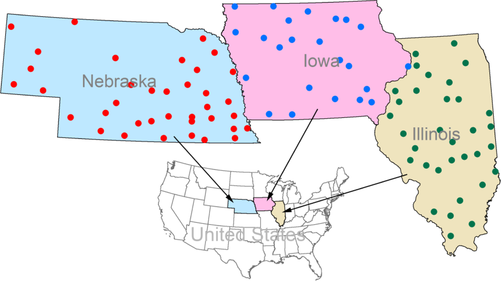
Figure 1.
Illustration of study area and selected meteorological stations. The study area covers three states of the United States: Iowa, Illinois and Nebraska. Stations are marked as circle dots, and colors are labeled for different states. The number of meteorological stations of Iowa (blue dots), Illinois (green dots), and Nebraska (red dots) is 23, 33, and 37, respectively.
Four kinds of data sets, as listed follows, spanning a decade (2002 throughout 2011) of corn growing seasons (the 13th week throughout the 47th week) are chosen for this study.
- (1)
- Daily NDVI time series, which is derived from the atmospherically corrected MODIS MOD09GQ (MODIS Surface Reflectance Daily L2G Global 250 m) dataset with 250 m spatial resolution. This data set is publicly available through the “Vegetation Condition Explorer” ( http://dss.csiss.gmu.edu/NDVIDownload/), maintained by the Center for Spatial Information Science and Systems (CSISS), George Mason University.
- (2)
- NASS’s Cropland Data Layer (CDL), which is a raster, geo-referenced crop-specific land use data layer. The spatial resolution of years 2006–2009 is 56 m, and the rest is 30 m. The data set is publicly available via “CropScape” ( http://nassgeodata.gmu.edu/), produced operationally by USDA/NASS.
- (3)
- NASS’s CPRs, which record the percent complete (area ratio) of crop fields that has either reached or completed a specific progress stage over a specific administrative unit. It is publicly available via NASS’s “Quick Stats 2.0” service ( http://www.nass.usda.gov/Quick_Stats/). More details of the first three data sets can refer to [19].
- (4)
- Daily minimum and maximum temperatures, which are derived from the United States Historical Climatology Network (USHCN) [27]. USHCN is a high-quality network of US Cooperative Observer Network stations, specially selected for analyzing long-term variability and change in the whole contiguous United States [27]. In this study, 23, 33, and 37 meteorological stations are chosen for the states of Iowa, Illinois, and Nebraska, respectively (Figure 1 and Appendix: Table A1). The meteorological stations were selected with a number of criteria including length of period of record, and spatial coverage.
3. Feature Extraction
Multisource features are used as the input of the HMM model. Global features, which are measured in the state-level, include mean NDVI, fractal dimension, and AGDDs. Along the corn life cycle, these features are in different forms of distribution (Figure 2). The mean NDVI and fractal dimension curves are unimodal and bimodal, respectively. The AGDDs is in a monotonic curve. Mean NDVI and fractal dimension are extracted from remote sensing image. AGDDs data are extracted from the site-specific observations of meteorological stations. The implementation of the feature extraction is introduced in the following subsections.
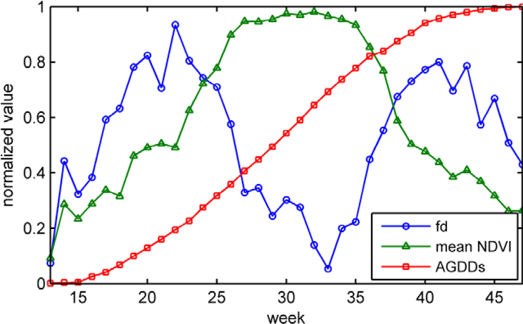
Figure 2.
Distributions of normalized mean Normalized Difference Vegetation Index (NDVI), fractal dimension (fd), and AGDDs along the corn life cycle (Iowa, 2007).
3.1. Mean NDVI
NDVI measures the greenness of crop on spectral response of remote sensing image. To extract the mean NDVI in the state-level, data pre-processing has been conducted over the original daily MODIS-NDVI time series. The data pre-processing mainly includes: image compositing, which composites daily NDVI images into weekly composite products by Maximum Value Composite (MVC) [28], and image masking, which eliminates non-corn pixels from weekly NDVI image with the mask of NASS’s CDL. Relevant agreements of the data pre-processing procedures can be found in [19]. Mean NDVI is extracted directly by statistics on masked weekly NDVI image. It is worth mentioning that no additional pre-process has been conducted on the time series, e.g., smoothing, and filtering.
3.2. Fractal Dimension
Fractal dimension measures the roughness of corn NDVI image, which can be used as an index of heterogeneity to reflect corn growth status. As stated in [19], roughness varies in the growth season due to corn fields are at different stages, i.e., fractal dimension time series reflects spatiotemporal changes of corn in the life cycle. The fractal dimension is estimated by Dimensionality-Reduction based Differential Box-Counting (DR-DBC) algorithm [19]. The estimation process is also conducted on the masked weekly NDVI image.
3.3. AGDDs
Photoperiod and temperature are two common environmental factors that significantly affect crop growth and development [29]. Modern corn hybrids are less vulnerable to photoperiod, but are greatly affected by temperature [29]. In the studies of crop growth, temperature is often presented as growing degree days. AGDDs, defined as an explanatory temperature variable from some consistent start date until a specific subsequent, are usually related to crop growth in the corn life cycle [6,7].
Ambient minimum and maximum temperatures are observed by meteorological station, i.e., the raw data are in the site-specific form. To extract the global AGDDs, two steps should be taken: (1) calculate the mean minimum/maximum temperature of state-level from site-specific observations; and (2) calculate AGDDs from adjusted mean minimum and maximum temperatures. We define daily minimum and maximum temperatures of the ith meteorological station at the Day of Year (DOY) t as
and
, respectively. The state-level mean minimum and maximum temperatures at the DOY t are defined as T̄min(t) and T̄max(t), respectively. In addition, to calculate the AGDDs, adjustment should be performed on T̄min(t) and T̄max(t) by the rules of corn response to temperature stress. The adjusted T̄min(t) and are defined as Tmin(t) and Tmax(t), respectively.
T̄min(t) and T̄max(t) are generated by weighted average of all available meteorological stations within the corresponding administrative border. The Thiessen polygon approach [30], a geospatial technique, is applied to graphically weight meteorological station data. In this approach, each station is weighted in direct proportion based on its area of influence in the total area of specified administrative unit. It assumes that any point of temperature condition is equal to that of the nearest station. We take the calculation of T̄min(t) as example, and T̄max(t) is the same. The T̄min(t) over a state is calculated by
where n is the number of available meteorological stations over the given state, e.g., state of Iowa, n = 23; wi is the weight of station i, which can be determined by its corresponding influence area of station i, i.e., wi=Ai/Atotal, where Atotal is the administrative area of the given state, and Ai represents the influence area of station i that is divided by Thiessen polygon. The methods we used for calculating T̄min(t) in this paper are especially applicable and useful to avoid the ambient temperature data, which may be missing from the time series of records in actual practice.
Growth and development in crops is temperature dependent. Development does not occur unless temperatures exceed a lower base temperature Tbase, and ceases as temperatures exceed an upper threshold [31]. In the United States, the usual low temperature stress of corn or base temperature Tbase is 10° [32]. In addition, previous studies have shown that corn growth slows at temperatures above 30° [32]. Therefore, we use 10° and 30° to adjust T̄min(t) and T̄max(t) accordingly. That is, if the lowest temperature for a day is below the 10°, then 10° is used as the Tmin(t), and if the highest temperature is over the 30°, then 30° is used as Tmax(t). Start date is set as 1 April. Given the T̄min(t) and T̄max(t), and according to the rule of adjustment, the AGDDs at the DOY can be calculated by
4. Corn Progress Percentages Estimation
As a doubly embedded stochastic process, HMM involves at least two levels of uncertainty: a hidden stochastic process that is not directly observable, but can be observed only through another set of stochastic processes that generate the sequence of observations [21]. In our model, the observable variables (multisource features) include mean NDVI, fractal dimension, and AGDDs, while the unobservable (hidden) variables are corn progress stages. In the following sections, we will introduce the HMM briefly, then focus on the estimation of corn progress percentages for any specified time, as soon as the remote sensing and meteorological data are available.
4.1. Specifying an HMM
Corn progress can be assumed as a Markov process with N hidden stages S = {S1, …, SN}, and T observation sequence O = {O1, …, OT}. In this study, the hidden stages consist of pre-season (S1), planted (S2), emerged (S3), silking (S4), dough (S5), dent (S6), mature (S7), and harvested (S8). The pre-season stage, which represents the period when corn hasn’t been planted, is added as the first time interval to facilitate the design of the model. Let qt, (t = 1, …, T) be a variable of the hidden stage at time t. For example, progress stage Si, (i = 1, …, N) at time t is denoted by qt = Si. Therefore, we can specify an HMM of a corn progress by its parameters λ = (A, B, Π), where A is the stage transition probability matrix whose entry, ai,j(t) = P(qt = Sj|qt–1 = Si), (i, j = 1, …, N) determines the transition probability from stage Si to stage Sj at time t; B is the observation probability matrix whose entry, bj (Ot) = P(Ot|qt = Sj), indicates the probability that the observation Ot are generated by the stage Sj at time t; Π is the initial probability distribution whose entry, πi = P(q1 = Si), determines the probability of the model being initially in stage Si at the first time node (i.e., t = 1). πi also represents the prior probability of stage Si at time t = 1. It can be extended by πi(t) = P(qt = Si) that represents the prior probability of Si at time t. The joint probability distribution over all of the variables is given by
where, r,j = 1, …, N.
In this study, the sequence q1, …, qt is assumed to be a typical Markov chain with a first-order Markov assumption, i.e., stage at qt can only be decided by stage of previous latent variable qt−1 and independent of all other stages. We abbreviate P(qt = Sj|qt−1 = Si) as ai,j(t). In addition, the observation Ot at time t can only be determined by its corresponding stage Sj. P(Ot|qt = Sj) is abbreviated as bj(Ot). Thus, the probability that mentioned in Equation (3) is also equal to
4.2. Mixture Model in HMMs
HMM could be understood as combining a Markov chain model with a mixture model [33]. Two embedded stochastic processes in the HMM related to two chains: the external chain of observations and the internal chain of hidden stages (Figure 3). It is capable to represent uncertainties on stage determination and on observation [26]. In addition, “HMMs viewed as mixture” [34] represents that observation at each time node might be impacted by multiple hidden stages, assuming observation that forms N clusters can be modeled as a mixture of N components. A single time node corresponds to a mixture distribution with component densities bi(Ot), i.e., each stage of discrete variable qt represents a different component. The probability of observation is given by
where, πi(t) can be regarded as the weight of the ith component, and
.
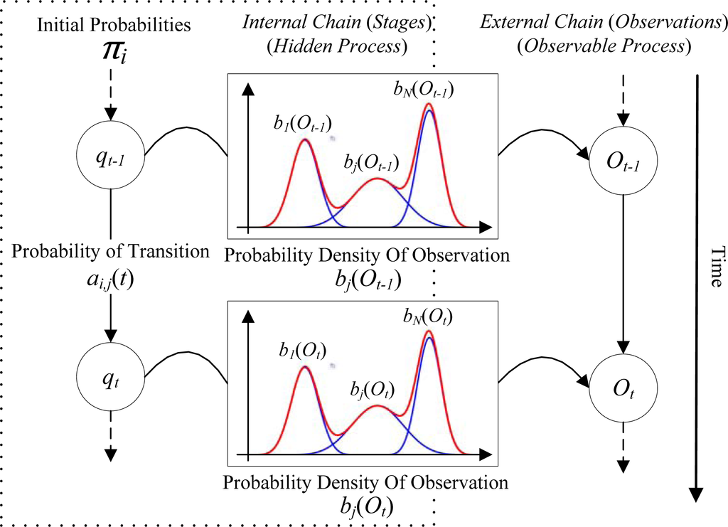
Figure 3.
Basic principle of proposed Hidden Markov Model (HMM).
Mixture model provides flexibility and precision in modeling the underlying statistics of corn progress stages. HMM uses discrete hidden stage representations. It is applicable to combine the hidden stage of continuous probability space models and the discrete stage of HMMs to model time series with continuous but nonlinear dynamics. In our case, the continuous observation HMM, the entry of bi(Ot) is given by continuous probability density functions, i.e., Gaussian distribution.
4.3. NASS’s CPRs Normalization
The NASS’s CPRs record the progress percentages of each growth stage by the percent complete (area ratio) in the ASD-level or state-level, e.g., percent complete of stage Si at time t noted as
, (i = 1, …, N). Ratios represent stages complete, rather than the proportion of each stage occupancy over an administrative unit in current time (Figure 4(a)). Corn phenological stages are unimodal in the life cycle. For a single corn plant, the arrival of Sj, (1 ≤ i < j ≤ N) means Si has already completed. That is, Si is nested within Sj, e.g., 19% of dough (S5) has completed means at least 19% of silking (S4) had completed already.
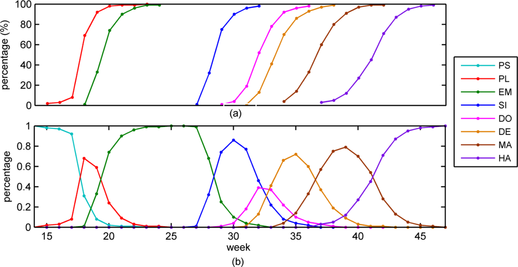
Figure 4.
NASS’s CPRs Normalization, Iowa (2011). PS = pre-season. PL = planted, EM = emerged, SI = silking, DO = dough, DE = dent, MA = mature, and HA = harvested. (a) original corn progress percentages; (b) normalized corn progress percentages.
In our model, the normalized CPRs or stage prior πi(t) can be straightforward to signify the area ratio of stage Si occupancy at time t for a specific administrative unit. Theoretically, πi(t) can be calculated from the original recording of NASS’s CPRs. It should be noted that some stages have no records of NASS’s CPRs data, because stage has not arrived or even passed by. Thus, before the πi(t) calculation, we need a data filling process for CPRs data. If the data recorded has not reached a certain stage, the value is set to 0, and if the developmental stage has passed, then the value is set to 1.
We assume that each stage can only transform up to itself or its next stage within a week, For example, in Figure 4, emerged (S3) takes at least 9.5 days (bigger than a week) delays after the planted (S2). Then, πi(t) is calculated by
For example, in the 31th week (Iowa, 2011) shown in Figure 4(a), stages of dent (S6), dough (S5) and silking (S4) have completed 1%, 19% and 96%, respectively. Based on Equation (6), we know that this region has 1%, 18%, 77% and 4% of corn plants at dent, dough silking and emerged (S3) stages, respectively (Figure 4(b)).
4.4. HMM Parameters Determination
As mentioned above, an HMM consists of three probabilities: initial probability distribution, stage transition probabilities, and observation probabilities. They can be estimated from archive data with the following processes.
4.4.1. Initial Probability Distribution
The initial probability distribution or stage prior probabilities, which specifies the onset time, characterizes the stage of model if observations are not taken into account [26]. To estimate the probability of each stage at the onset of growth season, we need a prior knowledge about preferential months for corn sowing [25]. Generally, the 13th week of our study area, is assumed at the pre-season stage for most corn plants. For practical applications, the initial probability can be calculated from the statistics on historical records at the same time slice, e.g., the initial stage probabilities of the 13th week are estimated by averaging of normalized records of NASS’s CPRs on all available years at the same week.
4.4.2. Stage Transition Probability Matrix
In conventional HMM, the stage transition probability matrix A with N × N is a global parameter, i.e., all weeks along the life cycle share the same transition probability matrix. However, this is not adapted to model corn growth. Transition probabilities should be allowed to vary, similarly to time inhomogeneous Markov chain [35]. The time-dependent transition probabilities also can be found in tumor expression profiles [36] and financial time-series data analysis [35]. In our case, the matrix A varies along corn growth. For example, at the start of the life cycle, corn is likely to be at the initial progress stage, i.e., the transition from current stage to itself is strong, and to its next stage is weak. However, with the time passes by, transition to initial progress stage becomes weak gradually, and then vanished. Generally, the transition variation depends on the biophysical mechanisms and external factors driving corn plant growth. The former depends greatly on characteristics of a particular crop, e.g., breeding [37]. The latter conditioned mostly by soil characteristics, elevation, irradiation, temperature, precipitation, and human disturbances as well [26].
We consider stage transition probability matrix as a local HMM parameter (time-dependent). The probability ai,j(t) varies when time t changes. We assume a life cycle is unimodal, i.e., stage Si only can transform to itself or its next stage Si+1 (Figure 5). ai,j(t) can be calculated directly from normalized NASS’s CPRs data. Thus, ai,j(t) is calculated by
where,
. i and j determine the position of stages with respect to the time variable t. There are four restrictions in Equation (7). The first three relate to self-transition probability at the end, self-transition probability in the chain, and forward stage change, respectively. For example, if qt−1 = S6, then all transitions except a6,6(t) and a6,7(t) are zero element. a6,6(t) and a6,7(t) respectively correspond to the second and third restrictions, which sum up to 1.
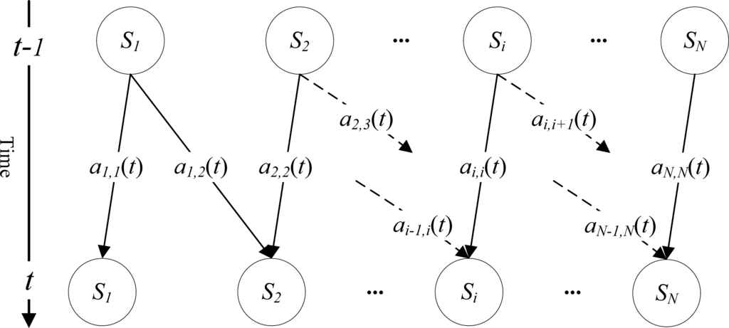
Figure 5.
Illustration of corn progress stage transition along a life cycle.
In practical applications, the stage probability transform matrix is determined through a two-step strategy as follows: (1) mean progress percentages are calculated by averaging of normalized recordings on all available years at each time slice; and (2) stage transform probability matrix of each time slice is calculated by Equation (7). The first averaging step will result in a certain degree of errors especially progress stages that are produced by unexpected factors, including climate change, farming practices, and natural disasters. However, the hidden stages in our HMM, which controlled by stage transition probabilities, are regarded as stochastic process and it is able to incorporate uncertainties.
4.4.3. Observation Probability Matrix
The probability of observation being generated in a certain stage is called the observation probability. In this paper, the feature vector is comprised of mean NDVI, fractal dimension, and AGDDs. Observation values continuously change with the effect of phenological alternation. Moreover, there would be multiple progress stages occupied in the same time period of an administrative unit. Thus, we model observation to be a mixture of stages (Figure 3). The mixing weights are determined by the area ratio of each stage occupation, which coincide with the prior probabilities of each stage πi(t). Probability density function associated with observations for each administrative unit can be modeled by a multivariate Gaussian distribution. Thus, in Equation (5), P(Ot) is a linear superposition of Gaussian distribution, and bi(Ot) is parameterized on mean vector μi and covariance matrix ∑i.bi(Ot) is given by
where, d refers to the dimensionality of the observation space, and d = 3 causing three kinds of features were selected in this study.
In our model, μi and ∑i are global HMM parameters, i.e., they are independent to time. The ith component weight (or mixing coefficient) πi(t) knowns from ground surveying, i.e., only μi and ∑i are unknown. Given an observation sequence O1, …, OT, we can determine μi and ∑i using maximum likelihood. The log-likelihood function with parameter space Θ = {μ, ∑}is given by
and it can be estimated by Expectation Maximization (EM) [38] iterative algorithm with E-step (expectation) and M-step (maximization). EM starts with initial values for the parameters μi and ∑i and iteratively performs these two steps until convergence to a local maximum of the likelihood function. In the (q + 1)th iteration, the
and
are calculated by
where
In our case, the observation probabilities are composed by eight Gaussian distribution components. We approximately assume
to initialize the
with Equation (10) and
with Equation (11), then iteratively perform EM algorithm until convergence to a local maximum. Meanwhile, we record the corresponding mean vector μi and covariance matrix ∑i during the last iteration.
4.5. Progress Percents Estimation
The goal of this paper is to determine the area proportion of each progress stage. This problem can be regarded as computing the posterior over the hidden stages at each time t, given HMM parameter λ, and all available observations up to the current time, e.g., P(qt = Sj|O1, …, Ot). This is an online process (real-time), and can be solved by filtering based algorithms. We should emphasize that filtering, smoothing (offline), and prediction problems all compute the probability of hidden stages for given observations, e.g., P(qt = Sj|O1, …, Oh). More specifically, the difference is the smoothing problem compute by t < h, the filtering t = h, and prediction t > h. We note P(qt = Sj, O1, …, Ot) as κj(t), which represents the probability of all the observation up to time t and the stage at time t is Sj, then
Generally, the forward algorithm is directly adapted to calculate κj(t) for the observation sequence of increasing interval t. Then, κj(t) can be obtained recursively according to
with the initial forward probabilities as the joint probability of state Sj and initial observation O1
After estimating P(qt = Sj|O1, …, Ot) which also represents area ratio of stage Sj occupancy at time t for a specific administrative unit, an inverse normalize transfer process should be deployed. We note δi(t) as the progress percent of stage Si at time t. Then it can be calculated by
where, i = 2, …, N.
5. Results and Discussions
By constructing a general HMM framework for corn progress stages estimation with multisource features, seven key corn progress stages and its percentages can be estimated in the real-time. Experiments have been conducted on the states of Iowa, Illinois, and Nebraska of the United States. A decadal data (2002 throughout 2011) during the corn growing seasons is selected for this study. The 13th week is set as the start date.
5.1. RMSE Results
The accuracy of the experiments is evaluated by Root Mean Squared Error (RMSE) [39], which measures the difference between estimated and observed values. The values in the following are expressed as a percentage, because the estimation results in corn progress percentages. Lower values indicate less residual variance. The evaluation covers the whole corn life cycle. The pre-season stage is not included in the error evaluation, because it is only defined to facilitate our model. Figure 6 shows the RMSE of all seven NASS/USDA defined corn progress stages in states of Iowa, Illinois, and Nebraska, respectively. All the results are the average of 100 runs. In each run, 7 year data are randomly selected for training, and remaining 3 year are used for testing. Results reported in error bar are significantly better, with confidence level 95%.
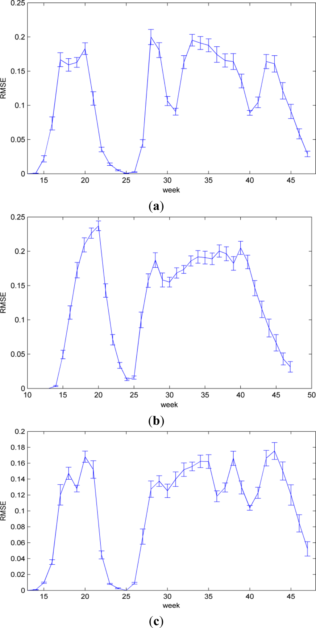
Figure 6.
RMSE of corn progress percentage estimates. (a) Iowa; (b) Illinois; (c) Nebraska.
By analyzing errors in the processing of stage percentages determination (Figure 6), we find that the RMSE increases gradually, and reaches the first greater maximum around the 20th week. The corresponding RMSE is 18.29% (Iowa), 23.71% (Illinois), and 16.82% (Nebraska). This is likely caused by the uncontrollable planting practices, e.g., different planting speed in different year. Then, the RMSE decreases gradually until the 25th week. By referring to Figure 4, we find that in this period the proportion of emerged stage increases gradually, and only emerged left around the 25th week. In the week, results are less affected by overlaps of stages. After the emerged stage, the RMSE reaches another maximum around the 28th week, and then fluctuates around 18.0% (Iowa), 18.5% (Illinois), and 16.5% (Nebraska) until the 43th week. This is likely caused by progress stage overlaps, e.g., harvest stage is overlapped with dented and mature stages. During this period, results will be more affected by model errors, which are generated in the parameters estimation of state transition probabilities and observation probabilities. In addition, the errors inherited from original data have also impacted the accuracy of estimation.
5.2. Accuracy Comparison
Although it is not the same case on the estimation of corn progress percentages, we try to find a comparable case to compare our method with spectral pixel-wise based method. Yu et al.[40] developed kernel-based methods to estimate the corn phenological stages that defined by NASS/USDA. The base kernel, which is determined from modeling annual NDVI profiles of previous years in the pixel-wise, is tolerant to noisy data and missing data. Comparison in different combinations on threshold (global or local), masking (percentage of pure pixels, e.g., 90% and 100%), and filter algorithms (e.g., quintic polynomial, double Sigmoid, Savitzky-Golay, and Spline) have been conducted. The test is conducted in the state of Iowa in year 2006. The study also gives the RMSE of modeled results against NASS’s CPRs for the whole year. The lowest RMSE is 24.6%, corresponding to the combination of local threshold, pure pixels and Spline-based smoothing method.
To perform better comparison with the results that presented in [40], we convert our weekly RMSE into whole year RMSE. Our result shows that the RMSE is 13.27% (Iowa), 16.14% (Illinois), and 12.91% (Nebraska). The comparison results indicate that our method is better than spectral pixel-wise based methods on the estimation of corn progress to some extent.
5.3. Performance and Analysis
One of the advantages of this method is that we can estimate the proportion of each corn progress stage in a real-time through the established model and the currently acquired data. The estimated results can correspond to NASS’s CPRs directly. The following factors can significantly impact the results.
- (1)
- The accuracy of NASS’s CPRs. The NASS’s CPRs are surveyed data, and mainly depended on the subjective assessment of investigators. Thus, a bias error is inevitably introduced in the NASS’s CPRs data [41];
- (2)
- The quality of MODIS NDVI. Noise has inevitably disturbed the daily MODIS-NDVI images, e.g., cloud cover, missing data, mixed pixels, or some of the systematic errors that reduce the index value of daily MODIS-NDVI images;
- (3)
- The reliability of meteorological data, regarding to the observation data of weather stations, data missing, instrumentation, or observation station location change may affect the data homogeneity and spatial coverage;
- (4)
- Irregularities in raining and temperature pattern in different years, e.g., extensive drought occurs in a particular year, can significantly affect the stability of results. It would specially impacted on HMM parameters training, e.g., the stage transition probability matrix.
- (5)
- The insufficiency of temporal resolution. The temporal resolution of data is an important factor that affects the accuracy of corn progress stages estimation. As shown in Figure 4, the emerged stage just 9.5 days delays to planted stage, and dent stage approximate 15.4 days delays to dough stage. Accurate distinction between these growth stages requires a higher temporal resolution. It is really intractable that we have to trade off temporal resolution and data quality.
There are many suggested ways, which would improve the accuracy of the results. One believes that although an image compositing process has been conducted and contributed to eliminate noises in this paper, more reliable quality control for original remote sensing data will suppress noises and improve the accuracy of the corn progress percentage estimation. Another potential solution is to use high-order HMMs. High-order stage transition dependency would result in good modeling of stage duration [42]. Mari et al. [43] carried out a comparative study between first- and second-order HMMs on automatic word recognition. Seifert et al. [44,45] utilized high-order HMM to improve modeling of spatial dependencies between chromosomal regions. Derrode et al. [46] introduced a high-order hidden Markov chain for unsupervised SAR image segmentation, which allows one to take into account more complex and correlated noise. Study on the applicability of high-order HMM for estimating corn progress stages is needed to further determine.
6. Conclusion
Remote sensing and meteorological data have been separately employed for detecting crop progress stages in most recent studies. In this paper, we have performed the integration of multisource data for retrieving corn progress metrics. Three features in the state-level have been chosen, including mean NDVI, fractal dimension, and AGDDs. The mean NDVI and fractal dimension are extracted from MODIS-NDVI, while the AGDDs derived from meteorological data. It is worth mentioning that the fractal dimension, which indicates the spatial pattern of remote sensing image, is used to measure the changes of corn crop along the life cycle. In order to estimate corn progress stages in the real-time, and directly relate to ground survey data, e.g., NASS’s CPRs, an HMM-based method has been proposed. The multisource features are considered as the input to the model, and no additional pre-process is conducted, e.g., smoothing, and filtering. It is also worth mentioning that the developed model is different from conventional HMM models in several aspects: (1) The stage transition probability matrix has been considered as a local HMM parameter, which is reasonable for modeling the growth of corn; (2) Because several stages may jointly affect the observation in the state-level at each time node, the observation probability matrix has been constructed with a mixture model, i.e., observation at each time node is viewed as the mixture of stages with Gaussian distribution. The modified HMM is suitable for estimating the corn progress percentages in the real-time. Experimental studies have been conducted in the states of Iowa, Illinois, and Nebraska of the United States. Comparisons between our method and a series of VIs time series based methods also have been implemented. The results demonstrate that the proposed method performed well on the real-time estimation of corn progress stages. The corn progress percentages can be estimated with accuracies of ±12.91%–16.14%, which is better than the results of spectral pixel-wise based methods (±24.6%). Although the described examples were performed on corn crop and the state-level data sets, the proposed method is also applicable for the real-time estimation of progress stages on other types of crop in multiple county-level.
Acknowledgments
The authors would like to acknowledge the valuable comments received from two anonymous reviewers that help in shaping the paper. They would also like to thank Qunying Huang of Department of Geography and Geoinformation Sciences, George Mason University, for editing and proofreading the paper.
This work is partially supported by grants from the National Basic Research Program of China (grant # 2011CB707102), the NASA Earth Science Application Program (grant # NNX09AO14G; PI: Liping Di), the Fundamental Research Funds for Central Universities (grant # 105565GK), the open research fund of Key Laboratory of Mine Spatial Information Technologies of the State Bureau of Surveying and Mapping, Henan Polytechnic University (grant # KLM201108 and # KLM201014), Gray Haze Remote Sensing Monitoring Technology Research and Operation Demonstration of JiangSu Province (grant # 201130), and China Scholarship Council (CSC).
References
- USDA-OCE: Weekly Weather and Crop Bulletin. Available online: http://www.usda.gov/oce/weather/pubs/Weekly/Wwcb/index.htm (accessed on 18 November 2012).
- Zhang, X.; Friedl, M.; Schaaf, M.; Strahler, A.H.; Hodges, J.C.F.; Gao, F.; Reed, B.C.; Huete, A. Monitoring vegetation phenology using MODIS. Remote Sens. Environ 2003, 84, 471–475. [Google Scholar]
- Hird, J.N.; McDermid, G.J. Noise reduction of NDVI time series: An empirical comparison of selected techniques. Remote Sens. Environ 2009, 113, 248–258. [Google Scholar]
- Atkinson, P.M.; Jeganathan, C.; Dash, J.; Atzberger, C. Inter-comparison of four models for smoothing satellite sensor time-series data to estimate vegetation phenology. Remote Sens. Environ 2012, 123, 400–417. [Google Scholar]
- Ricotta, C.; Avena, G.C. The remote sensing approach in broad-scale phenological studies. Appl. Veg. Sci 2000, 3, 117–122. [Google Scholar]
- Sasaoka, K.; Chiba, S.; Saino, T. Climatic forcing and phytoplankton phenology over the subarctic north pacific from 1998 to 2006, as observed from ocean color data. Geophys. Res. Lett 2011. [Google Scholar] [CrossRef]
- White, M.A.; de Beurs, K.M.; Didan, K.; Inouye, D.W.; Richardson, A.D.; Jensen, O.P.; O’Keefe, J.; Zhang, G.; Nemani, R.R.; van LeeuWen, W.J.D.; et al. Intercomparison, interpretation, and assessment of spring phenology in north america estimated from remote sensing for 1982–2006. Glob. Chang. Biol 2009, 15, 2335–2359. [Google Scholar]
- Diepen, C.A.; Wolf, J.; van Keulen, H. WOFOST: A simulation model of crop production. Soil Use Manage 1989, 5, 16–24. [Google Scholar]
- Stöckle, C.O.; Donatelli, M.; Nelson, R. Cropsyst, a cropping systems simulation model. Eur. J. Agron 2003, 18, 289–307. [Google Scholar]
- Jones, J.W.; Tsuji, G.Y.; Hoogenboom, G.; Hunt, L.A.; Thornton, P.K.; Wilkens, P.W.; Imamura, D.T.; Bowen, W.T.; Singh, U. Decision Support System for Agrotechnology Transfer: DSSAT V3. In Understanding Options for Agricultural Production; Tsuji, G.Y., Hoogenboom, G., Thornton, P., Eds.; Kluwer Academic Publishers: Boston, MA, USA, 1998; pp. 157–177. [Google Scholar]
- Saxton, K.E.; Porterand, M.A.; McMahon, T.A. Climatic impacts on dryland winter wheat by daily soil water and crop stress simulations. Agr. For. Meteorol 1992, 58, 177–192. [Google Scholar]
- Kroes, J.G.; Dam, J.C.V.; Groenendijk, P.; Hendriks, R.F.A.; Jacobs, C.M.J. SWAP Version 3.2: Theory Description and User Manual; Alterra Report; Alterra: Wageningen, The Netherlands, 2008. [Google Scholar]
- De Beurs, K.M.; Henebry, G.M. Spatio-Temporal Statistical Methods for Modelling Land Surface Phenology. In Phenological Research: Methods for Environmental and Climate Change Analysis; Hudson, I.L., Keatley, M.R., Eds.; Springer-Verlag: New York, NY, USA, 2010. [Google Scholar]
- Toukiloglou, P. Comparison of AVHRR, MODIS and VEGETATION for Land Cover Mapping and Drought Monitoring at 1 km Spatial Resolution. 2007. [Google Scholar]
- Reed, B.C.; Brown, J.F.; Vanderzee, D.; Loveland, T.R.; Merchant, J.W.; Donald, D.O. Measuring phenological variability from satellite imagery. J. Veg. Sci 1994, 5, 703–714. [Google Scholar]
- Ren, J.; Chen, Z.; Zhou, Q. Regional yield estimation for winter wheat with MODIS-NDVI data in Shandong, China. Int. J. Appl. Earth Obs. Geoinf 2008, 10, 403–413. [Google Scholar]
- Atzberger, C. Advances in remote sensing of agriculture: Context description, existing operational monitoring systems and major information needs. Remote Sens 2013, 5, 949–981. [Google Scholar]
- Culbert, P.D.; Pidgeon, A.M.; Louis, V.S.; Bash, D.; Radeloff, V.C. The impact of phenological variation on texture measures of remotely sensed imagery. IEEE J. Sel. Top. Appl. Earth Observ 2009, 2, 299–309. [Google Scholar]
- Shen, Y.; Di, L.; Yu, G.; Wu, L. Correlation between corn progress stages and fractal dimension from MODIS-NDVI time series. IEEE Geosci. Remote Sens. Lett 2013, 10, 1–5. [Google Scholar]
- USDA-NASS: National Crop Progress Terms and Definitions. Available online: http://www.nass.usda.gov/Publications/NationalCropProgress/TermsandDefinitions/index.asp (accessed on 18 November 2012).
- Elliott, R.J.; Siu, T.K. An HMM approach for optimal investment of an insurer. Int. J. Robust Nonlinear Contr 2012, 22, 778–807. [Google Scholar]
- Rabiner, L.R. A tutorial on hidden Markov models and selected applications in speech recognition. Proc. IEEE 1989, 77, 257–286. [Google Scholar]
- Krogh, A.; Brown, M.; Mian, I.S.; Sjölander, K.; Haussler, D. Hidden Markov models in computational biology: Applications to protein modeling. J. Mol. Biol 1994, 235, 1501–1531. [Google Scholar]
- Aurdal, L.; Bang, H.R.; Eikvil, L.; Solberg, R.; Vikhamar, D.; Solberg, A. Hidden Markov Models Applied to Vegetation Dynamics Analysis Using Satellite Remote Sensing. Proceedings of International Workshop on the Analysis of Multi-Temporal Remote Sensing Images, Biloxi, MS, USA, 16–18 May 2005; pp. 220–224.
- Leite, P.; Feitosa, R.; Formaggio, A.; Costa, G.; Pakzad, K.; Sanches, I. Hidden Markov models for crop recognition in remote sensing image sequences. Pattern Recognition Lett 2011, 32, 19–26. [Google Scholar]
- Viovy, N.; Saint, G. Hidden Markov models applied to vegetation dynamics analysis using satellite remote sensing. IEEE Trans. Geosci. Remote Sens 1994, 32, 906–917. [Google Scholar]
- The United States Historical Climatology Network (USHCN). Available online: http://cdiac.ornl.gov/epubs/ndp/ushcn/ushcn.html (accessed on 18 November 2012).
- Holben, B.N. Characteristics of maximum-value composite images from temporal AVHRR data. Int. J. Remote Sens 1986, 7, 1417–1434. [Google Scholar]
- Wiebold, B. Growing Degree Days and Corn Maturity; Technical Report; University of Missouri: Columbia, MO, USA, 2002. [Google Scholar]
- Thiessen, A.H. Precipitation averages for large areas. Mon. Wea. Rev 1911, 39, 1082–1089. [Google Scholar]
- Trudgill, D.L.; Honek, A.; Li, D.; van Straalen, N.M. Thermal time-concepts and utility. Ann. Appl. Biol 2005, 146, 1–14. [Google Scholar]
- McMaster, G.S.; Wilhelm, W.W. Growing degree-days: One equation, two interpretations. Agr. Forest Meteorol 1997, 87, 291–300. [Google Scholar]
- Jaakkola, T.S. Machine Learning, Lecture Notes 19: Hidden Markov Models (HMMs). 2006. Available online: http://ocw.mit.edu/courses/electrical-engineering-and-computer-science/6-867-machine-learning-fall-2006/lecture-notes/lec19.pdf (accessed on 18 November 2012).
- Srihari, S.N. Machine Learning and Probabilistic Graphical Models Course: Hidden Markov Models. 2011. Available online: http://www.cedar.buffalo.edu/srihari/CSE574/index.html (accessed on 18 November 2012).
- Knab, B.; Schliep, A.; Steckemetz, B.; Wichern, B. Model-Based Clustering with Hidden Markov Models and its Application to Financial Time-Series Data. In Between Data Science and Applied Data Analysis; Schader, M., Gaul, W., Vichi, M., Eds.; Springer: New York, NY, USA, 2003; pp. 561–569. [Google Scholar]
- Seifert, M.; Strickert, M.; Schliep, A.; Grosse, I. Exploiting prior knowledge and gene distances in the analysis of tumor expression profiles with extended Hidden Markov Models. Bioinformatics 2011, 27, 1645–1652. [Google Scholar]
- Sacks, W.J.; Kucharik, C.J. Crop management and phenology trends in the U.S. corn belt: Impacts on yields, evapotranspiration and energy balance. Agr. Forest Meteorol 2011, 151, 882–894. [Google Scholar]
- Dempster, A.P.; Laird, N.M.; Rubin, D.B. Maximum likelihood from incomplete data via the EM algorithm. J. Roy. Stat. Soc. B 1977, 39, 1–38. [Google Scholar]
- Heij, C.; de Boer, P.; Franses, P.H.; Kloek, T.; van Dijk, H.K. Econometric Methods with Applications in Business and Economics; Oxford University Press Inc: New York, NY, USA, 2004. [Google Scholar]
- Yu, G.; Di, L.; Yang, Z.; Shen, Y.; Zhang, B.; Chen, Z. Corn Growth Stage Estimation Using Time Series Vegetation Index. Proceedings of 2012 First International Conference on Agro-Geoinformatics (Agro-Geoinformatics), Shanghai, China, 2–4 August 2012; pp. 1–6.
- Sakamoto, T.; Wardlow, B.D.; Gitelson, A.A. Detecting spatiotemporal changes of corn developmental stages in the U.S. corn belt using MODIS WDRVI data. IEEE Trans. Geosci. Remote Sens 2011, 49, 1926–1936. [Google Scholar]
- Lee, L. High-order hidden Markov model and application to continuous mandarin digit recognition. J. Inf. Sci. Eng 2011, 27, 1919–1930. [Google Scholar]
- Mari, J.F.; Haton, J.P.; Kriouile, A. Automatic word recognition based on second-order hidden Markov models. IEEE Trans. Speech Audio Proc 1997, 5, 22–25. [Google Scholar]
- Seifert, M.; Cortijo, S.; Colomé-Tatché, M.; Johannes, Frank; Roudier, F.; Colot, V. MeDIP-HMM: Genome-wide identification of distinct DNA methylation states from high-density tiling arrays. Bioinformatics 2012. [Google Scholar] [CrossRef]
- Seifert, M.; Gohr, A.; Strickert, M.; Grosse, I. Parsimonious higher-order hidden Markov models for improved array-CGH analysis with applications to Arabidopsis thaliana. PLoS Comp. Biol 2012, 8, 1–15. [Google Scholar]
- Derrode, S.; Carincotte, C.; Bourennane, S. Unsupervised Image Segmentation Based on High-Order Hidden MARKOV Chains. Proceedings of IEEE International Conference on Acoustics, Speech, and Signal Processing (ICASSP), Marseille, France, 17–21 May 2004; pp. 769–772.
Appendix

Table A1.
Basic information of selected meteorological stations. Meteorological data include ID, name, and the geographic coordinate (i.e., latitude, longitude, and elevation) of each station. SA means US state abbreviations.
| No | ID | SA | Name | Lat (°N) | Lon (°W) | Elev (m) | No | ID | SA | Name | Lat (°N) | Lon (°W) | Elev (m) |
|---|---|---|---|---|---|---|---|---|---|---|---|---|---|
| 1 | 130112 | IA | ALBIA 3 NNE | 41.07 | 92.79 | 268.2 | 48 | 116579 | IL | PANA 3E | 39.37 | 89.02 | 213.4 |
| 2 | 130133 | IA | ALGONA 3 W | 43.07 | 94.31 | 377.6 | 49 | 116610 | IL | PARIS WTR WKS | 39.64 | 87.69 | 207.3 |
| 3 | 130600 | IA | BELLE PLAINE | 41.88 | 92.28 | 246.9 | 50 | 116910 | IL | PONTIAC | 40.89 | 88.64 | 198.1 |
| 4 | 131402 | IA | CHARLES CITY | 43.08 | 92.67 | 309.1 | 51 | 117551 | IL | RUSHVILLE | 40.12 | 90.56 | 201.2 |
| 5 | 131533 | IA | CLARINDA | 40.72 | 95.02 | 298.7 | 52 | 118147 | IL | SPARTA 1 W | 38.12 | 89.72 | 163.1 |
| 6 | 131635 | IA | CLINTON #1 | 41.79 | 90.26 | 178.3 | 53 | 118740 | IL | URBANA | 40.08 | 88.24 | 219.8 |
| 7 | 132724 | IA | ESTHERVILLE 2 N | 43.43 | 94.82 | 396.8 | 54 | 118916 | IL | WALNUT | 41.55 | 89.6 | 210.3 |
| 8 | 132789 | IA | FAIRFIELD | 41.02 | 91.96 | 225.6 | 55 | 119241 | IL | WHITE HALL 1 E | 39.44 | 90.38 | 176.8 |
| 9 | 132864 | IA | FAYETTE | 42.85 | 91.82 | 344.4 | 56 | 119354 | IL | WINDSOR | 39.44 | 88.6 | 210.3 |
| 10 | 132977 | IA | FOREST CITY 2 NNE | 43.28 | 93.63 | 396.2 | 57 | 250130 | NE | ALLIANCE 1WNW | 42.11 | 102.9 | 1,217.4 |
| 11 | 132999 | IA | FORT DODGE 5NNW | 42.58 | 94.2 | 347.5 | 58 | 250375 | NE | ASHLAND NO 2 | 41.04 | 96.38 | 326.1 |
| 12 | 134063 | IA | INDIANOLA 2W | 41.37 | 93.65 | 287.1 | 59 | 250435 | NE | AUBURN 5 ESE | 40.37 | 95.75 | 283.5 |
| 13 | 134142 | IA | IOWA FALLS | 42.52 | 93.25 | 344.4 | 60 | 250640 | NE | BEAVER CITY | 40.13 | 99.83 | 658.4 |
| 14 | 134735 | IA | LE MARS | 42.78 | 96.15 | 364.2 | 61 | 251145 | NE | BRIDGEPORT | 41.67 | 103.1 | 1,117.4 |
| 15 | 134894 | IA | LOGAN | 41.64 | 95.79 | 301.8 | 62 | 251200 | NE | BROKEN BOW 2 W | 41.41 | 99.68 | 762 |
| 16 | 135769 | IA | MT AYR | 40.71 | 94.24 | 359.7 | 63 | 252020 | NE | CRETE | 40.62 | 96.95 | 437.4 |
| 17 | 135796 | IA | MT PLEASANT 1 SSW | 40.95 | 91.56 | 222.5 | 64 | 252100 | NE | CURTIS 3NNE | 40.67 | 100.49 | 829.4 |
| 18 | 135952 | IA | NEW HAMPTON | 43.05 | 92.31 | 349.9 | 65 | 252205 | NE | DAVID CITY | 41.25 | 97.13 | 490.7 |
| 19 | 137147 | IA | ROCK RAPIDS | 43.43 | 96.17 | 411.5 | 66 | 252820 | NE | FAIRBURY 5S | 40.07 | 97.17 | 411.5 |
| 20 | 137161 | IA | ROCKWELL CITY | 42.4 | 94.63 | 364.2 | 67 | 252840 | NE | FAIRMONT | 40.64 | 97.59 | 499.9 |
| 21 | 137979 | IA | STORM LAKE 2 E | 42.63 | 95.17 | 434.3 | 68 | 253175 | NE | GENEVA | 40.53 | 97.6 | 496.8 |
| 22 | 138296 | IA | TOLEDO 3N | 42.04 | 92.58 | 289.3 | 69 | 253185 | NE | GENOA 2 W | 41.45 | 97.76 | 484.6 |
| 23 | 138688 | IA | WASHINGTON | 41.28 | 91.71 | 210.3 | 70 | 253365 | NE | GOTHENBURG | 40.94 | 100.15 | 787.9 |
| 24 | 110072 | IL | ALEDO | 41.2 | 90.75 | 219.5 | 71 | 253615 | NE | HARRISON | 42.69 | 103.88 | 1,478.3 |
| 25 | 110187 | IL | ANNA 2 NNE | 37.48 | 89.23 | 195.1 | 72 | 253630 | NE | HARTINGTON | 42.62 | 97.26 | 417.6 |
| 26 | 110338 | IL | AURORA | 41.78 | 88.31 | 201.2 | 73 | 253660 | NE | HASTINGS 4N | 40.65 | 98.38 | 591.3 |
| 27 | 111280 | IL | CARLINVILLE | 39.29 | 89.87 | 189.3 | 74 | 253735 | NE | HEBRON | 40.18 | 97.59 | 451.1 |
| 28 | 111436 | IL | CHARLESTON | 39.48 | 88.17 | 198.1 | 75 | 253910 | NE | HOLDREGE | 40.45 | 99.38 | 707.1 |
| 29 | 112140 | IL | DANVILLE | 40.14 | 87.65 | 170.1 | 76 | 254110 | NE | IMPERIAL | 40.52 | 101.66 | 999.7 |
| 30 | 112193 | IL | DECATUR WTP | 39.83 | 88.95 | 189 | 77 | 254440 | NE | KIMBALL 2NE | 41.25 | 103.63 | 1,435 |
| 31 | 112483 | IL | DU QUOIN 4 SE | 37.99 | 89.19 | 128 | 78 | 254900 | NE | LODGEPOLE | 41.15 | 102.64 | 1,168 |
| 32 | 113335 | IL | GALVA | 41.17 | 90.04 | 246.9 | 79 | 254985 | NE | LOUP CITY | 41.28 | 98.97 | 627.3 |
| 33 | 113879 | IL | HARRISBURG | 37.74 | 88.52 | 111.3 | 80 | 255080 | NE | MADISON | 41.83 | 97.45 | 481.6 |
| 34 | 114108 | IL | HILLSBORO | 39.15 | 89.48 | 192 | 81 | 255310 | NE | MC COOK | 40.22 | 100.62 | 796.1 |
| 35 | 114198 | IL | HOOPESTON 1 NE | 40.47 | 87.66 | 216.4 | 82 | 255470 | NE | MERRIMAN | 42.92 | 101.71 | 986 |
| 36 | 114442 | IL | JACKSONVILLE 2E | 39.73 | 90.2 | 185.9 | 83 | 255565 | NE | MINDEN | 40.52 | 98.95 | 658.4 |
| 37 | 114823 | IL | LA HARPE | 40.58 | 90.97 | 210.3 | 84 | 256135 | NE | OAKDALE | 42.07 | 97.97 | 521.2 |
| 38 | 115079 | IL | LINCOLN | 40.15 | 89.34 | 177.7 | 85 | 256570 | NE | PAWNEE CITY | 40.12 | 96.16 | 378 |
| 39 | 115326 | IL | MARENGO | 42.29 | 88.65 | 248.4 | 86 | 256970 | NE | PURDUM | 42.07 | 100.25 | 819.9 |
| 40 | 115712 | IL | MINONK | 40.91 | 89.03 | 228.6 | 87 | 257070 | NE | RED CLOUD | 40.1 | 98.52 | 524.3 |
| 41 | 115768 | IL | MONMOUTH | 40.92 | 90.64 | 227.1 | 88 | 257515 | NE | SAINT PAUL 4N | 41.27 | 98.47 | 541 |
| 42 | 115833 | IL | MORRISON | 41.80 | 89.97 | 183.8 | 89 | 257715 | NE | SEWARD | 40.9 | 97.09 | 438.9 |
| 43 | 115901 | IL | MT CARROLL | 42.1 | 89.98 | 195.1 | 90 | 258395 | NE | SYRACUSE | 40.68 | 96.19 | 335.3 |
| 44 | 115943 | IL | MT VERNON 3 NE | 38.35 | 88.85 | 149.4 | 91 | 258465 | NE | TECUMSEH 1S | 40.35 | 96.19 | 338.3 |
| 45 | 116446 | IL | OLNEY 2S | 38.7 | 88.08 | 146.3 | 92 | 258480 | NE | TEKAMAH | 41.79 | 96.23 | 338.3 |
| 46 | 116526 | IL | OTTAWA 5SW | 41.33 | 88.91 | 160 | 93 | 258915 | NE | WAKEFIELD | 42.27 | 96.86 | 423.7 |
| 47 | 116558 | IL | PALESTINE | 39 | 87.62 | 140.2 |