Article

Segmentation Based Classification of 3D Urban Point Clouds: A Super-Voxel Based Approach with Evaluation

by
Ahmad Kamal Aijazi
1,2,
Paul Checchin
1,2,* and
Laurent Trassoudaine
1,2
1
Institut Pascal, Clermont Université, Université Blaise Pascal, BP 10448, F-63000 Clermont-Ferrand, France
2
Institut Pascal, CNRS, UMR 6602, F-63171 Aubière, France
*
Author to whom correspondence should be addressed.
Remote Sens. 2013, 5(4), 1624-1650; https://doi.org/10.3390/rs5041624
Submission received: 12 January 2013 / Revised: 6 March 2013 / Accepted: 13 March 2013 / Published: 28 March 2013
(This article belongs to the Special Issue Advances in Mobile Laser Scanning and Mobile Mapping)

Abstract

:
Segmentation and classification of urban range data into different object classes have several challenges due to certain properties of the data, such as density variation, inconsistencies due to missing data and the large data size that require heavy computation and large memory. A method to classify urban scenes based on a super-voxel segmentation of sparse 3D data obtained from LiDAR sensors is presented. The 3D point cloud is first segmented into voxels, which are then characterized by several attributes transforming them into super-voxels. These are joined together by using a link-chain method rather than the usual region growing algorithm to create objects. These objects are then classified using geometrical models and local descriptors. In order to evaluate the results, a new metric that combines both segmentation and classification results simultaneously is presented. The effects of voxel size and incorporation of RGB color and laser reflectance intensity on the classification results are also discussed. The method is evaluated on standard data sets using different metrics to demonstrate its efficacy.

Graphical Abstract

1. Introduction

The automatic segmentation and classification of 3D urban data have gained widespread interest and importance in the scientific community due to the increasing demand of urban landscape analysis and cartography for different popular applications, coupled with the advances in 3D data acquisition technology. The automatic extraction (or partially supervised) of important urban scene structures such as roads, vegetation, lamp posts, and buildings from 3D data has been found to be an attractive approach to urban scene analysis, because it can tremendously reduce the resources required for analyzing the data for subsequent use in 3D city modeling and other algorithms.
A common way to quickly collect 3D data of urban environments is by using an airborne LiDAR [1,2], where the LiDAR scanner is mounted in the bottom of an aircraft. Although this method generates a 3D scan in a very short time period, there are a number of limitations in 3D urban data collected from this method, such as a limited viewing angle. These limitations are overcome by using a mobile terrestrial or ground based LiDAR system in which, unlike the airborne LiDAR system, the 3D data obtained is dense and the point of view of the images is closer to the urban landscapes. However, this leads to both advantages and disadvantages when processing the data. The disadvantages include the demand for more processing power required to handle the increased volume of 3D data. On the other hand, the advantage is the availability of a more detailed sampling of the object’s lateral views, which provides a more comprehensive model of the urban structures including building facades, lamp posts, etc.
Over the last few years an important number of projects has been undertaken globally to analyze and model 3D urban environments. The presented work is also realized as part of the French government project ANR iSpace&Time, which involves classification, modeling and simulation of urban environment for 4D Visualization of cities.
Our work revolves around the segmentation and then classification of ground based 3D data of urban scenes. The aim is to provide an effective pre-processing step for different subsequent algorithms or as an add-on boost for more specific classification algorithms. The main contribution of our work includes: (1) a voxel based segmentation using a proposed Link-Chain method; (2) classification of these segmented objects using geometrical features and local descriptors; (3) introduction of a new evaluation metric that combines both segmentation and classification results simultaneously; (4) evaluation of the proposed algorithm on standard data sets using 3 different evaluation methods; (5) study of the effect of voxel size on the classification accuracy; (6) study of the effect of incorporating reflectance intensity with RGB color on the classification results.

2. Related Work

In the context of the proposed work, the literature review presented here is divided into two main sections: segmentation and classification. In each of these sections the relevant work is discussed and grouped under different techniques used in these domains.

2.1. Segmentation of 3D Data

In order to fully exploit 3D point clouds, for scene understanding and object classification, effective segmentation has proved to be a necessary and critical pre-processing step in a number of autonomous perception tasks.

2.1.1. Specialized Features and Surface Discontinuities

Earlier works including [3,4] employed the use of small sets of specialized features, such as local point density or height from the ground, to discriminate only few object categories in outdoor scenes, or to separate foreground from background. In literature survey, we also find some segmentation methods based on surface discontinuities such as Moosman et al. [5], who used surface convexity in a terrain mesh as a separator between objects.

2.1.2. Graph Clustering

Lately, segmentation has been commonly formulated as graph clustering. Instances of such approaches are Graph-Cuts including Normalized-Cuts and Min-Cuts. Golovinskiy and Funkhouser [6] extended Graph-Cuts segmentation to 3D point clouds by using k-Nearest Neighbors (k-NN) to build a 3D graph. In this work, edge weights based on exponential decay in length were used. But the limitation of this method is that it requires prior knowledge of the location of the objects to be segmented.
Another segmentation algorithm for natural images, introduced by Felzenszwalb and Huttenlocher (FH) [7], has gained popularity for several robotic applications due to its efficiency. This algorithm makes simple greedy decisions, and yet produces segmentations that satisfy the global properties by using a particular region comparison function that measures the evidence for a boundary between pairs of regions. Zhu et al. [8] presented a method in which a 3D graph is built with k-NN while assuming the ground to be flat for removal during pre-processing. 3D partitioning is then obtained with the FH algorithm. We have used the same assumption.
Triebel et al. [9] modified the FH algorithm for range images to propose an unsupervised probabilistic segmentation technique. In this approach, the 3D data is first over-segmented during pre-processing. Schoenberg et al. [10] have applied the FH algorithm to colored 3D data obtained from a co-registered camera laser pair. The edge weights are computed as a weighted combination of Euclidean distances, pixel intensity differences and angles between surface normals estimated at each 3D point. The FH algorithm is then run on the image graph to provide the final 3D partitioning. The evaluation of the algorithm is done on road segments only.
Strom et al. [11] proposed a similar approach but modified the FH algorithm to incorporate angle differences between surface normals in addition to the differences in color values. Segmentation evaluation was done visually without ground truth data. Our approach differs from the abovementioned methods as, instead of using the properties of each point for segmentation resulting in over segmentation, we have grouped the 3D points based on Euclidian distance into voxels and then assigned normalized properties to these voxels transforming them into super-voxels. This not only prevents over segmentation but in fact reduces the data set by many folds thus reducing post-processing time.

2.1.3. Geometrical Primitives

A spanning tree approach to the segmentation of 3D point clouds was proposed in [12]. Graph nodes represent Gaussian ellipsoids as geometric primitives. These ellipsoids are then merged using a tree growing algorithm. The resulting segmentation is similar to a super-voxel type of partitioning with voxels of ellipsoidal shapes and various sizes. Unlike this method, our approach uses cuboids of different shapes and sizes as geometric primitives and a link-chain method to group them together.

2.1.4. Markov Random Fields

In the literature review, we also find some techniques, such as [13,14], that segment and label 3D points by employing Markov Random Fields to model their relationship in the local vicinity. These techniques proved to outperform classifiers based only on local features, but at a cost of computational time. Different methods such as [15] have been introduced to increase the efficiency.

2.2. Classification of 3D Data

In the past, research related to 3D urban scene classification and analysis had been mostly performed using either 3D data collected by airborne LiDAR for extracting bare-earth and building structures [16,17] or 3D data collected from static terrestrial laser scanners for extraction of building features such as walls and windows [18]. Recently, classification of urban environment using data obtained from mobile terrestrial platforms (such as [19]) has gained much interest in the scientific community due to the ever increasing demand of realistic 3D models for different popular applications coupled with the recent advancements in the 3D data acquisition technology.

2.2.1. Discriminate Models and Model Fitting

In [20] a method of multi-scale Conditional Random Fields is proposed to classify 3D outdoor terrestrial laser scanned data by introducing regional edge potentials in addition to the local edge and node potentials in the multi-scale Conditional Random Fields. This is followed by fitting Plane patches onto the labeled objects such as building terrain and floor data using the RANSAC algorithm as a post-processing step to geometrically model the scene. In [21] the authors extracted roads and objects just around the roads like road signs. They used a least square fit plane and RANSAC method to first extract a plane from the points followed by a Kalman filter to extract roads in an urban environment. Douillard et al. [22] presented a method in which 3D points are projected onto the image to find regions of interest for classification. Object classification is implemented using a rule based system to combine binary deterministic and probabilistic features.

2.2.2. Features Based

A method of classification based on global features is presented in [23] in which a single global spin image for every object is used to detect cars in the scene, while in [24] a Fast Point Feature Histogram (FPFH) local feature is modified into global feature for simultaneous object identification and view-point detection. Classification using local features and descriptors such as Spin Image [25], Spherical Harmonic Descriptors [26], Heat Kernel Signatures [27], Shape Distributions [28], 3D SURF feature [29] is also found in the literature survey. In [30], the authors use both local and global features in a combination of bottom-up and top-down processes. In this approach, spin images are used as local descriptors to classify cars in the scene in the bottom-up stage while Extended Gaussian Images are used as global descriptors for verification in the top-down stage. The work shows that the combination of local and global descriptors provides a good trade-off between efficiency and accuracy. There is also a third type of classification based on Bag Of Features (BOF) as discussed in [31].
In our work, we use geometrical models based on local features and descriptors to successfully classify different segmented objects represented by groups of voxels in the urban scene. Ground is assumed to be flat and is used as an object separator. Our segmentation technique is discussed in Section 3. Section 4 deals with the classification of these segmented objects. In Section 5, a new evaluation metric is introduced to evaluate both segmentation and classification together while, in Section 6, we present the results of our work. Finally, we conclude in Section 7.

3. Voxel Based Segmentation

The proposed voxel based segmentation method consists of three main parts, which are the voxelisation of data, the transformation of voxels into super-voxels and the clustering by link-chain method.

3.1. Voxelisation of Data

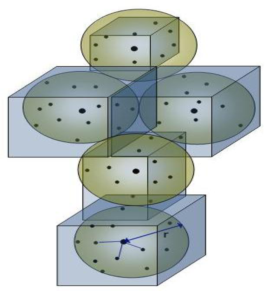
When dealing with large 3D data sets, the computational cost of processing all individual points is very high, making it impractical for real time applications. It is therefore sought to reduce these points by grouping together or removing redundant or un-useful points. Similarly, in our work the individual 3D points are clustered together to form a higher level representation or voxel as shown in Figure 1.
For p data points, a number of s voxels, where s << p, are computed based on r-NN, where r is the radius of ellipsoid. The maximum size of the voxel 2r depends upon the density of the 3D point cloud (the choice of this maximum voxel size is discussed in Section 6.5). In order to create the voxels, first a 3D point is selected as centre and using an r-NN with a fixed diameter (equal to maximum voxel size), all the 3D points in the vicinity are selected. All these 3D points now belong to this first voxel. Then, based on the maximum and minimum values of the 3D points contained in this voxel, the actual voxel size is determined. The same step is then repeated for other 3D points that are not part of the earlier voxel until all 3D points are considered (see Algorithm 1). In [20], color values are also added in this step but it is observed that for relatively smaller voxel sizes, the variation in properties such as color is not profound and just increases computational cost. For these reasons, we have only used distance as a parameter in this step. The other properties are used in the next step of clustering the voxels to form objects. Also we have ensured that each 3D point that belongs to a voxel is not considered for further voxelisation. This not only prevents over segmentation but also reduces processing time.
Algorithm 1. Segmentation
1:repeat
2:  Select a 3D point for voxelisation
3:  Find all neighboring points to be included in the voxel using r-NN within the specified maximum voxel length
4:  Transform voxel into s-voxel by first finding and then assigning to it all the properties found by using PCA, including surface normal.
5:until all 3D points are used in a voxel
6:repeat
7:  Specify an s-voxel as a principal link
8:  Find all secondary links attached to the principal link
9:until all s-voxels are used
10:Link all principal links to form a chain removing redundant links in the process
For the voxels we use a cuboid because of its symmetry, as it avoids fitting problems while grouping and also minimizes the effect of voxel shape during feature extraction. Although the maximum voxel size is predefined, the actual voxel sizes vary according to the maximum and minimum values of the neighboring points found along each axis to ensure the profile of the structure.

3.2. Transformation of Voxels into Super-Voxels

A voxel is transformed into a super-voxel when properties based on its constituting points are assigned to it. These properties mainly include:
  • VX,Y,Z: geometrical center of the voxel;
  • VR,G,B: mean R, G, & B value of constituting 3D points;
  • Var(R, G, B): maximum of the variance of R, G & B values;
  • VI: mean laser reflectance intensity value of constituting 3D points;
  • Var(I): variance of laser reflectance intensity values;
  • sX,Y,Z is the voxel size along each axis X, Y & Z;
  • Surface normals: A surface normal is calculated using PCA (Principal Component Analysis). The PCA method has been proved to perform better than the area averaging method [32] to estimate the surface normal. Given a point cloud data set 𝒟 = { x i } i = 1 n, the PCA surface normal approximation for a given data point p𝒟 is typically computed by first determining the k-Nearest Neighbors, xk𝒟, of p. Given the K neighbors, the approximate surface normal is then the eigenvector associated with the smallest eigenvalue of the symmetric positive semi-definite matrix
    P = k = 1 K ( x k p ¯ ) T ( x k p ¯ )
    where is the local data centroid: p ¯ = 1 K j = 1 K x j.
    The estimated surface normal is ambiguous in terms of sign; to account for this ambiguity it is homogenized using the dot product. Yet for us the sign of the normal vector is not important as we are more interested in the orientation. A surface normal is estimated for all the points belonging to a voxel and is then associated with that particular voxel.
With the assignment of all these properties, a voxel is transformed into a super-voxel. All these properties would then be used in grouping these super-voxels (from now onwards referred to as s-voxels) into objects and then during the classification of these objects.
Instead of using thousands of points in the data set, the advantage of this approach is that we can now use the reduced number of s-voxels to obtain similar results for classification and other algorithms. In our case, the data sets of 110, 392, 53, 676 and 27, 396 points were reduced to 18, 541, 6, 928 and 7, 924 s-voxels respectively, which were then used for subsequent processing.

3.3. Clustering by Link-Chain Method

When the 3D data is converted into s-voxels, the next step is to group these s-voxels to segment into distinct objects. Usually for such tasks, a region growing algorithm [33] is used in which the properties of the whole growing region may influence the boundary or edge conditions. This may sometimes lead to erroneous segmentation. Also common in such type of methods is a node based approach [5] in which at every node, boundary conditions have to be checked in all 5 different possible directions. In our work, we have proposed a link-chain method instead to group these s-voxels together into segmented objects.
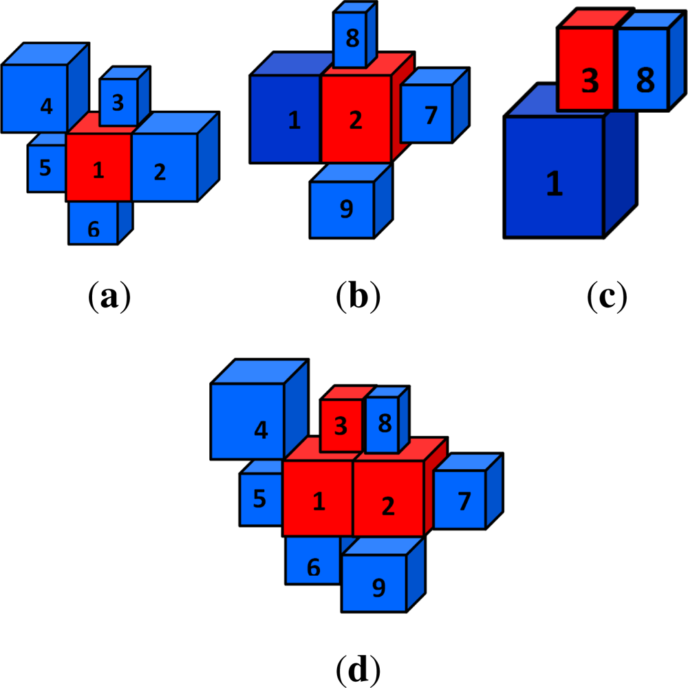
In this method, each s-voxel is considered as a link of a chain. Unlike the classical region growing algorithm, where a region is progressively grown from a seed (carefully selected start point), in the proposed method any s-voxel can be taken as a principal link and all secondary links attached to this principal link are found. The same is repeated for all s-voxels till all s-voxels are taken into account (see Algorithm 1 for details). Thus there is no need of a specific start point, no preference for choice of principal link nor any directional constraint, etc. In the final step, all the principal links are linked together to form a continuous chain removing redundant secondary links in the process as shown in Figure 2. These clusters of s-voxels represent the segmented objects.
Let VP be a principal link and Vn be the nth secondary link. Each Vn is linked to VP if and only if the following three conditions are fulfilled:
| V P X , Y , Z V n X , Y , Z | ( w D + c D )
| V P R , G , B V n R , G , B | 3 w C
| V P I V n I | 3 w I
where, for the principal and secondary link s-voxels respectively:
  • VPX,Y,Z, VnX,Y,Z are the geometrical centers;
  • VPR,G,B, VnR,G,B are the mean R, G & B values;
  • VPI, VnI are the mean laser reflectance intensity values;
  • wC is the color weight equal to the maximum value of the two variances Var(R, G, B), i.e., max(VPVar(R,G,B), VnVar(R,G,B));
  • wI is the intensity weight equal to the maximum value of the two variances Var(I).
wD is the distance weight given as ( V P s X , Y , Z + V n s X , Y , Z ) 2. Here sX,Y,Z is the voxel size along X, Y & Z axis respectively. cD is the inter-distance constant (along the three dimensions) added depending upon the density of points and also to overcome measurement errors, holes and occlusions, etc. The value of cD needs to be carefully selected depending upon the data (see Section 6.5 for more details on the selection of this value). The orientation of normals is not considered in this stage to allow the segmentation of complete 3D objects as one entity instead of just planar faces.
This segmentation method ensures that only the adjacent boundary conditions are considered for segmentation with no influence of a distant neighbor’s properties. This may prove to be more adapted to sharp structural changes in the urban environment. An overview of the segmentation method is presented in Algorithm 1. The programming structure adopted for implementation is based on standard graph-based algorithms [34].
With this method 18, 541, 6, 928 and 7, 924 s-voxels obtained from processing 3 different data sets were successfully segmented into 237, 75 and 41 distinct objects respectively.

4. Classification of Segmented Objects

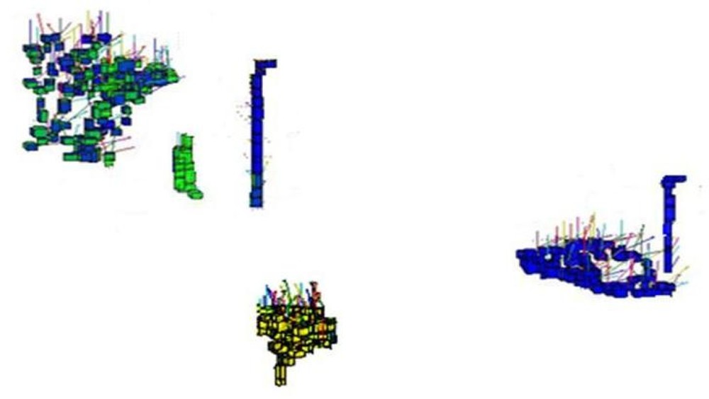
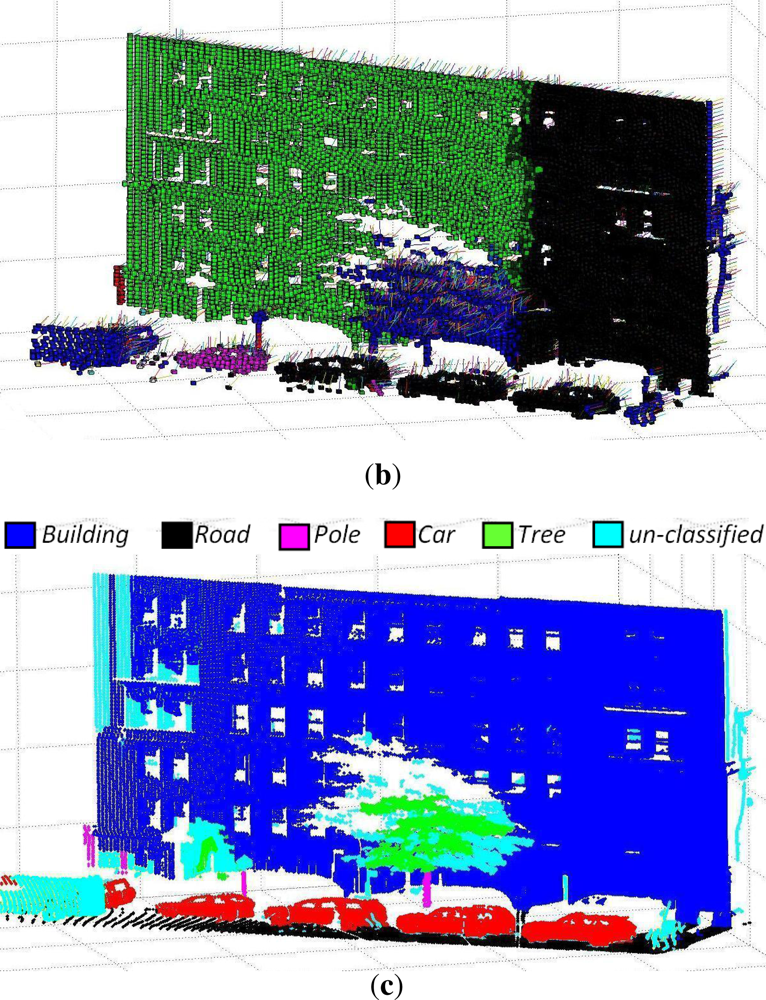
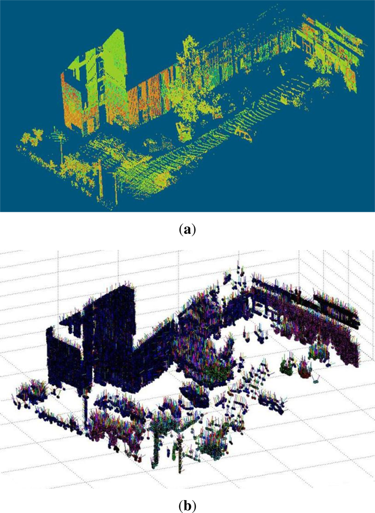
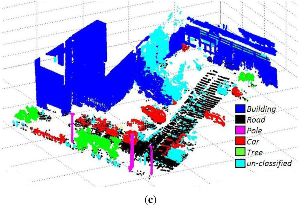
In order to classify these segmented objects, we assume the ground to be flat and use it as separator between objects. For this purpose we first classify and segment out the ground from the scene and then the rest of the objects. This step leaves the remaining objects as if suspended in space, i.e., distinct and well separated, making them easier to be classified as shown in Figure 3. In order to classify these segmented objects, a method is used that compares the geometrical models and local descriptors of these already segmented objects with a set of standard, predefined thresholds. The object types are so distinctly different that a simple choice of values for these differentiating thresholds is sufficient.
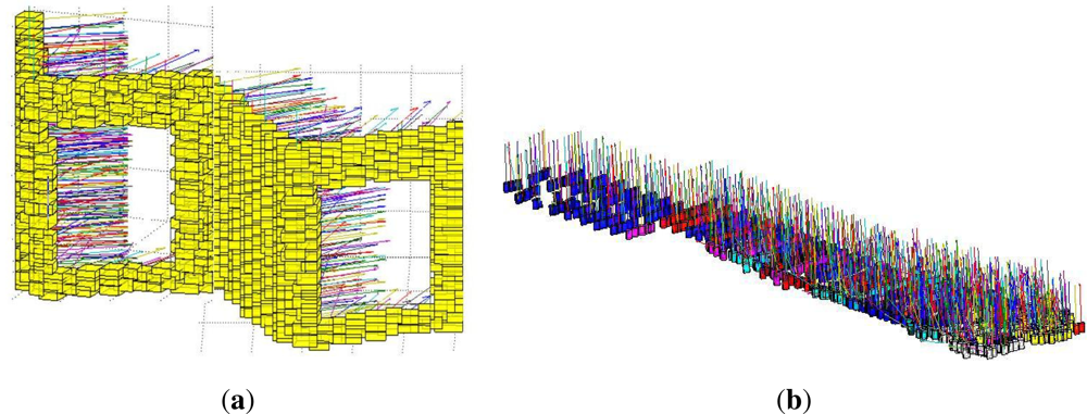
The ground or roads followed by these objects are classified using geometrical and local descriptors based on the constituting super-voxels. These mainly include:
a.
Surface normals: The orientation of the surface normals is found essential for the classification of ground and building faces. For ground object the surface normals are predominantly (threshold values greater than 80%) along Z-axis (height axis), whereas for building faces the surface normals are predominantly (threshold values greater than 80%) parallel to the X-Y axis (ground plane), see Figure 4.
b.
Geometrical center and barycenter: The height difference between the geometrical center and the barycenter along with other properties is very useful in distinguishing objects like trees and vegetation, etc., where h( barycenter − geometrical center) > 0, with h being the height function.
c.
Color and intensity: Intensity and color are also an important discriminating factor for several objects.
d.
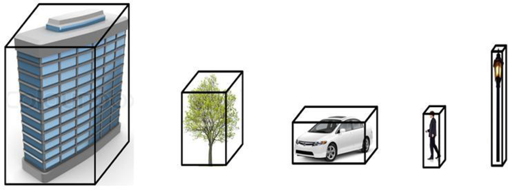
Geometrical shape: Along with the abovementioned descriptors, geometrical shape plays an important role in classifying objects. In 3D space, where pedestrians and poles are represented as long and thin with poles being longer, cars and vegetation are broad and short. Similarly, as roads represent a low flat plane, the buildings are represented as large (both in width and height) vertical blocks (as shown in Figure 5). The values for these comparison threshold on the shape and size for each of the object types are set accordingly.
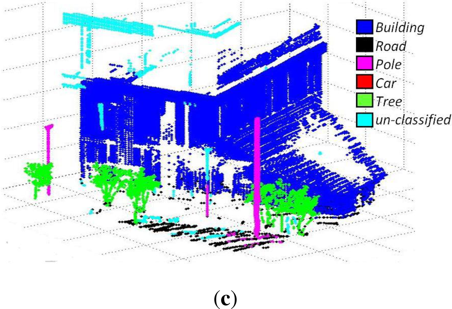
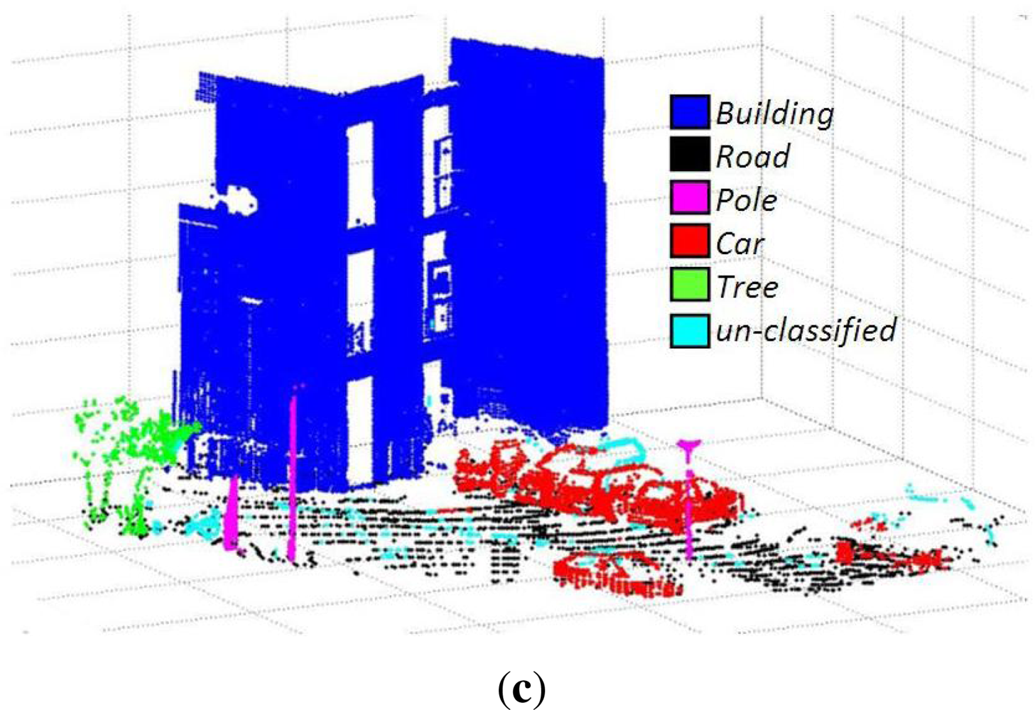
Using these descriptors we successfully classify urban scenes into 5 different classes (mostly present in our scenes), i.e., buildings, roads, cars, poles and trees. The object types chosen for classification are so distinctly different that if they are correctly segmented out, a simple classification method like the one proposed may be sufficient. The classification results and a new evaluation metric are discussed in the following sections.

5. Evaluation Metrics

Over the years, as new segmentation and classification methods are introduced, different evaluation metrics have been proposed to evaluate their performances. In previous works, different evaluation metrics are introduced for both segmentation results and classifiers independently. Thus in our work we present a new evaluation metric that incorporates both segmentation and classification together.
The evaluation method is based on comparing the total percentage of s-voxels successfully classified as a particular object. Let Ti, i ∈ {1, ⋯ , N}, be the total number of s-voxels distributed into objects belonging to N number of different classes, i.e., this serves as the ground truth, and let tji, i ∈ {1, ⋯ , N}, be the total number of s-voxels classified as a particular class of type-j and distributed into objects belonging to N different classes (for example an s-voxel classified as part of the building class may actually belong to a tree). Then the ratio Sjk (j is the class type as well as the row number of the matrix and k ∈ {1, ⋯ , N}) is given as:
S j k = t j k T k
These values of Sjk are calculated for each type of class and are used to fill up each element of the confusion matrix, row by row (refer to tables in Section 6.1 for instance). Each row of the matrix represents a particular class.
Thus, for a class of type-1 (i.e., first row of the matrix) the values of:
  • True Positive rate TP = S11 (i.e., the diagonal of the matrix represents the TPs)
  • False Positive rate FP = m = 2 N S 1 m
  • True Negative rate TN = (1 − FP)
  • False Negative rate FN = (1 − TP)
The diagonal of this matrix or TPs gives the Segmentation ACCuracy (SACC), similar to the voxel scores recently introduced by Douillard et al. [35]. The effects of unclassified s-voxels are automatically incorporated in the segmentation accuracy. Using the above values, the Classification ACCuracy (CACC) is given as:
CACC = TP + TN TP + TN + FP + FN
This value of CACC is calculated for all N types of classes of objects present in the scene. Overall Classification ACCuracy (OCACC) can then be calculated as
OCACC = 1 N i = 1 N CACC i
where N is the total number of object classes present in the scene. Similarly, the Overall Segmentation ACCuracy (OSACC) can also be calculated. The values of Ti and tji used above are laboriously evaluated by hand matching the voxelised data output and the final classified s-voxels and points.

6. Results

In order to test our algorithm two different data sets were used:
  • 3D data sets of Blaise Pascal University;
  • 3D Urban Data Challenge data set [36].
The 3D Urban Data challenge data set not only is one of the most recent data set but also contains the corresponding RGB and reflectance intensity values necessary to validate the proposed method. The proposed method is also suitable and well adapted for directly geo-referenced 3D point clouds obtained from mobile data acquisition and mapping techniques [37].

6.1. 3D Data Sets of Blaise Pascal University

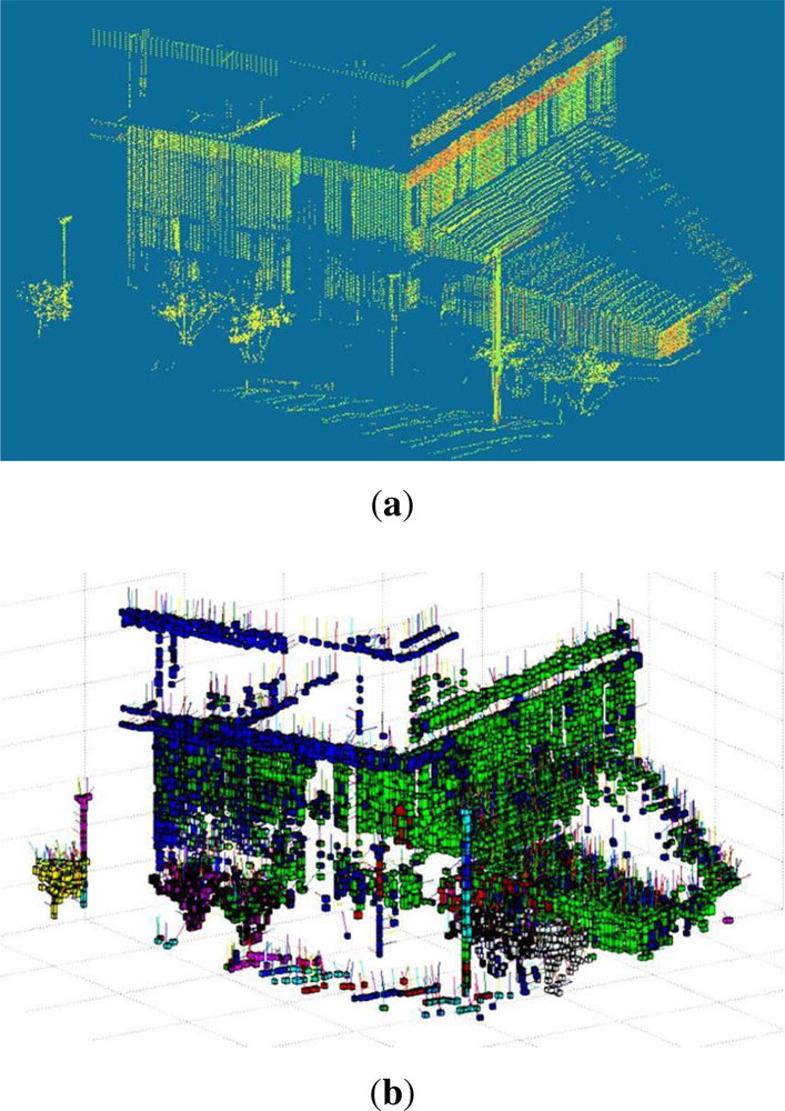
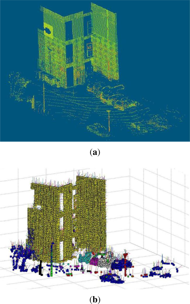
These data sets consist of 3D data acquired from different urban scenes on the Campus of Blaise Pascal University in Clermont-Ferrand, France, using a LEICA HDS-3000 3D laser scanner. The results of three such data sets are discussed here. The data sets consist of 27, 396, 53, 676 and 110, 392 3D points respectively. These 3D points were coupled with corresponding RGB and reflectance intensity values. The results are summarized in Table 1 and shown in Figures 6, 7 and 8 respectively. The evaluation results using the new evaluation metrics for the three data sets are presented in Tables 2, 3 and 4 respectively. These results are evaluated using a value of maximum voxel size equal to 0.3 m and cD = 0.25 m.

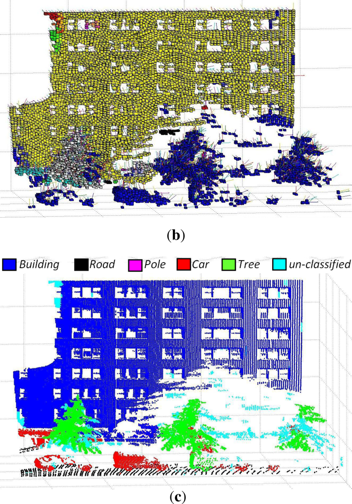
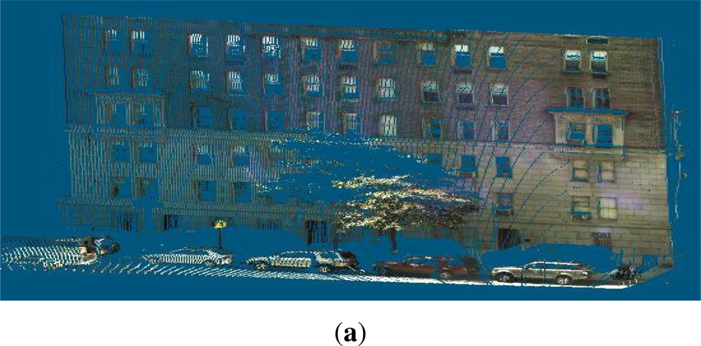
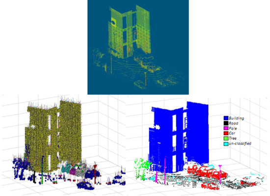
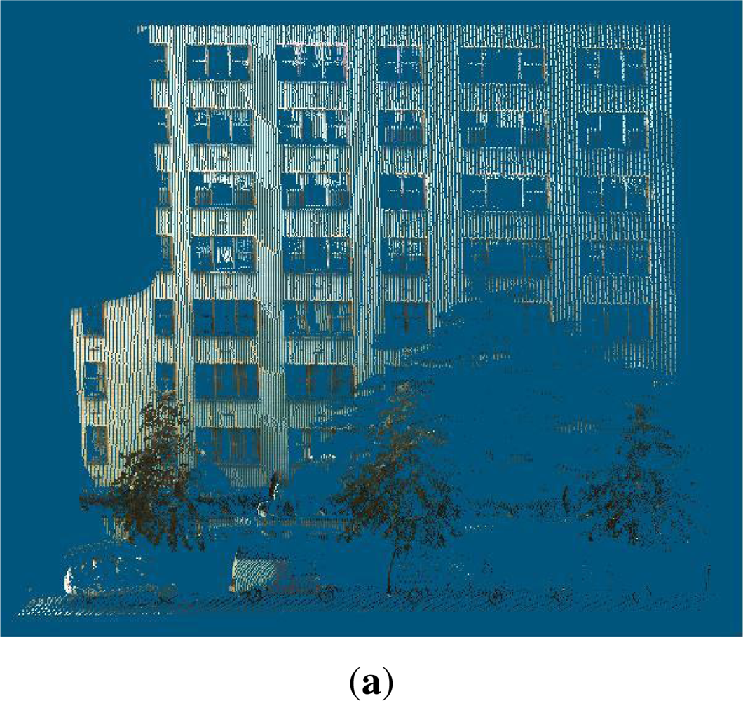
6.2. 3D Urban Data Challenge Data Set

The algorithm was further tested on the data set of the recently concluded 3D Urban Data Challenge 2011, acquired and used by the authors of [36]. This standard data set contains a rich collection of 3D urban scenes of the New York city mainly focusing on building facades and structures. These 3D points are coupled with the corresponding RGB and reflectance intensity values. A value of maximum voxel size equal to 0.5 m and cD = 0.15 m were used for this data set. Results (image results will be available in our website along with performance measures for comparison, after paper acceptance) of different scenes from this data set are shown in Figures 9, 10 and 11 and Tables 5, 6 and 7.

6.3. Comparison of Results with Existing Evaluation Methods

The classification results were also evaluated using already existing methods along with the proposed evaluation metrics for comparison purpose. Firstly, F-measure is used, which is one of the more frequently used metrics based on the calculation of Recall and Precision as described in [38]. Secondly, V-measure is used, which is a conditional entropy based metrics based on the calculation of Homogeneity and Completeness as presented in [39]. The later method overcomes the problem of matching suffered by the former and evaluates a solution independent of the algorithm, size of the data set, number of classes and number of clusters as explained in [39]. Another advantage of using these two metrics is that, just like the proposed metrics, they have the same bounded score. For all three metrics, the score varies from 0 to 1 and higher score signifies better classification results and vice versa. The results are summarized in Table 8.
From Table 8 it can be seen that the results evaluated by all three evaluation metrics are consistent with data set 2 receiving the highest scores and data set 3 the lowest. The results not only validate the proposed metrics but also indicate that it can be used as an alternative evaluation method. The results evaluated using these standard existing evaluation methods also permits to compare the performance of the proposed algorithm with other published techniques evaluated using them.

6.4. Performance Evaluation and Discussion

The proposed method gives good (in terms of scores) segmentation and classification results in all three evaluation methods. In general, the classification accuracy (OCACC) was found to be slightly better than the segmentation accuracy (OSACC). Not taking anything away from the segmentation method, one of the main reasons is that the 5 types of objects chosen for classification are distinctly different and that if the segmentation is good, classification becomes easier and a simple method like the one proposed is sufficient.
As compared with V-measure, the proposed method of evaluation can provide more information regarding individual segmentation and classification results (SACC and CACC). These results show that in most of the cases, the buildings, roads and poles have been classified the best with consistent scores of SACC and CACC higher than 90%, except in the case of data set 3 in which the building classification accuracy CACC is slightly deteriorated due to a large overlapping tree that is wrongly classified as a building rather than a tree. This is also reflected in the low Homogeneity value of 0.670 obtained when calculating V-measure for this data set. The classification of cars is generally good and the results are consistent but they are slightly hampered due to occlusions in some scenes (data set 3: CACC 86.3%, Scene B: CACC 89.5%). In case of trees, the SACC and CACC are found to vary the most. This is mainly due to the fact that the proposed classification method is based on local descriptors and geometrical features, which in the case of trees are very difficult to define (due to large variation of shapes, sizes and types). Thus, where the proposed algorithm succeeded in classifying smaller trees of more classical shapes with higher SACC and CACC scores, it produced low SACC and CACC scores of 68% and 79.4% respectively for Scene B. The Recall and Precision scores obtained during the calculation of F-measure for the tree class of this scene were found to be similarly low as well (0.682 and 0.614 respectively).

6.5. Effect of Voxel Size on Classification Accuracy and Choice of Optimal Values

Because the properties of s-voxels are constant mainly over the whole voxel length and these properties are then used for segmentation and classification, their size impacts the classification process. However, as the voxel size changes, the inter-distance constant cD also needs to be adjusted accordingly.
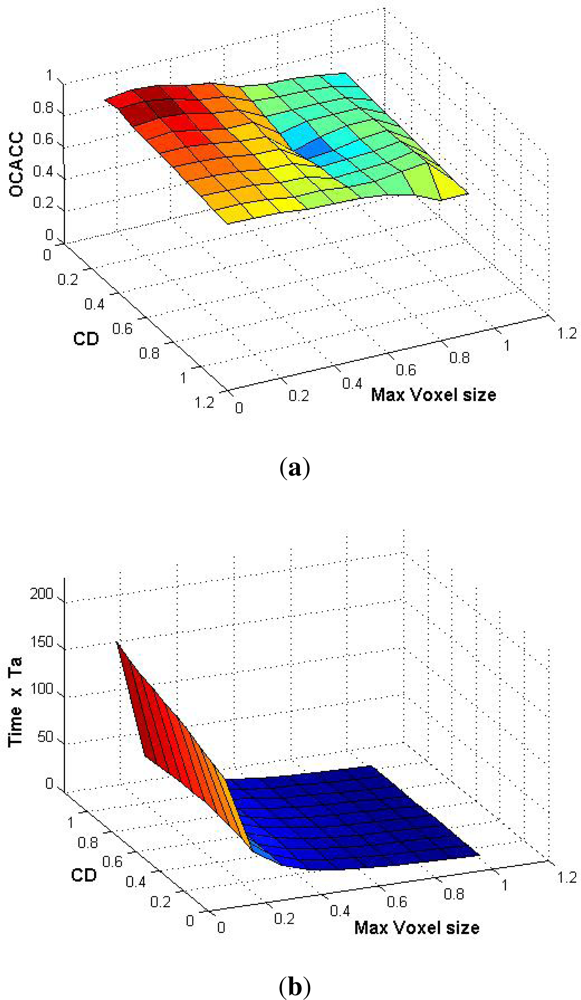
The effect of voxel size on the classification result was studied. The maximum voxel size and the value of cD were varied from 0.1 m to 1.0 m on data set 1 and corresponding classification accuracy was calculated. The results are shown in Figure 12(a). Then for the same variation of maximum voxel size and cD, the variation in processing time was studied as shown in Figure 12(b).
An arbitrary value of time Ta is chosen for comparison purposes (along Z-axis time varies from 0 to 200Ta). This makes the comparison results independent of the processor used, even though the same computer was used for all computations.
The results show that with smaller voxel size the segmentation and classification results are improved (with a suitable value of cD) but the computational cost increases. It is also evident that variation in value of cD has no significant impact on time t. It is also observed that after a certain reduction in voxel size, the classification result does not improve much but the computational cost continues to increase manifolds. As both OCACC and time (both plotted along Z-axis) are independent, using and combining the results of the two 3D plots in Figure 12 we can find the optimal value (in terms of OCACC and t) of maximum voxel size and cD depending upon the final application requirements. For our work, we have chosen a maximum voxel size of 0.3 m and cD = 0.25 m.

6.6. Influence of RGB Color and Reflectance Intensity

The effect of incorporating RGB Color and reflectance intensity values on the segmentation and classification was also studied. The results are presented in Table 9.
It is observed that incorporating RGB color alone is not sufficient in an urban environment due to the fact that it is heavily affected by illumination variation (part of an object may be under shade or reflect bright sunlight) even in the same scene. This deteriorates the segmentation process and hence the classification. This is perhaps responsible for the lower classification accuracy as seen in the first part of Table 9. It is the reason why intensity values are incorporated as they are more illumination invariant and found to be more consistent. The improved classification results are presented in the second part of Table 9.

6.7. Considerations for Further Improvements

The evaluated results of the proposed method on real and standard data sets show great promise. In order to complete this performance evaluation, comparison with other existing segmentation and classification methods is underway. While the method has successfully classified the urban environment into 5 basic object classes, an extension of this method to introduce more object classes is also being considered. One possible way could be to increase the number of features being used and train the classifier.

7. Conclusions

In this work we have presented a super-voxel based segmentation and classification method for 3D urban scenes. For segmentation a link-chain method is proposed. It is followed by the classification of objects using local descriptors and geometrical models. In order to evaluate our work we have introduced a new evaluation metric that incorporates both segmentation and classification results. The results show an overall segmentation accuracy (OSACC) of 87% and an overall classification accuracy (OCACC) of about 90%. The results indicate that with good segmentation, a simplified classification method like the one proposed is sufficient.
Our study shows that the classification accuracy improves by reducing voxel size (with an appropriate value of cD) but at the cost of processing time. Thus a choice of an optimal value, as discussed, is recommended. The study also demonstrates the importance of using laser reflectance intensity values along with RGB colors in the segmentation and classification of urban environment, as they are more illumination invariant and more consistent.
The proposed method can also be used as an add-on boost for other classification algorithms.

Acknowledgments

This work is supported by the Agence Nationale de la Recherche (ANR-the French national research agency) (ANR CONTINT iSpace & Time–ANR-10-CONT-23) and by “le Conseil Général de l’Allier”. The authors would like to thank Pierre Bonnet and all the other members of Institut Pascal who contributed to this project.

References

  1. Sithole, G.; Vosselman, G. Experimental comparison of filter algorithms for bare-Earth extraction from airborne laser scanning point clouds. ISPRS J. Photogramm 2004, 59, 85–101. [Google Scholar]
  2. Verma, V.; Kumar, R.; Hsu, S. 3D Building Detection and Modeling From Aerial Lidar Data. Proceedings of IEEE Computer Society Conference on the Computer Vision and Pattern Recognition, New York, NY, USA, 17–22 June 2006; 2, pp. 2213–2220.
  3. Rabbani, T.; van Den Heuvel, F.; Vosselmann, G. Segmentation of point clouds using smoothness constraint. Int. Arch. Photogramm. Remote Sens. Spatial Inf. Sci 2006, 36, 248–253. [Google Scholar]
  4. Sithole, G.; Vosselman, G. Automatic Structure Detection in a Point-Cloud of an Urban Landscape. Proceedings of 2nd GRSS/ISPRS Joint Workshop on the Remote Sensing and Data Fusion over Urban Areas, Venezia, Italy, 22–23 May 2003; pp. 67–71.
  5. Moosmann, F.; Pink, O.; Stiller, C. Segmentation of 3D Lidar Data in non-flat Urban Environments Using a Local Convexity Criterion. Proceedings of the IEEE Intelligent Vehicles Symposium (IV), Shaanxi, China, 3–5 June 2009; pp. 215–220.
  6. Golovinskiy, A.; Funkhouser, T. Min-Cut Based Segmentation of Point Clouds. Proceedings of the IEEE Workshop on Search in 3D and Video (S3DV) at ICCV, Nara, Japan, 29 September–2 October 2009; pp. 39–46.
  7. Felzenszwalb, P.; Huttenlocher, D. Efficient graph-based image segmentation. Int. J. Comput. Vision 2004, 59, 167–181. [Google Scholar]
  8. Zhu, X.; Zhao, H.; Liu, Y.; Zhao, Y.; Zha, H. Segmentation and Classification of Range Image from an Intelligent Vehicle in Urban Environment. Proceedings of the IEEE/RSJ International Conference on Intelligent Robots and Systems (IROS), Taipei, Taiwan, 18–22 October 2010; pp. 1457–1462.
  9. Triebel, R.; Shin, J.; Siegwart, R. Segmentation and Unsupervised Part-Based Discovery of Repetitive Objects. Proceedings of the Robotics: Science and Systems, Zaragoza, Spain, 27–30 June 2010; p. 8.
  10. Schoenberg, J.; Nathan, A.; Campbell, M. Segmentation of Dense Range Information in Complex Urban Scenes. Proceedings of the IEEE/RSJ International Conference on Intelligent Robots and Systems (IROS), Taipei, Taiwan, 18–22 October 2010; pp. 2033–2038.
  11. Strom, J.; Richardson, A.; Olson, E. Graph-Based Segmentation for Colored 3D Laser Point Clouds. Proceedings of the IEEE/RSJ International Conference on Intelligent Robots and Systems (IROS), Taipei, Taiwan, 18–22 October 2010; pp. 2131–2136.
  12. Pauling, F.; Bosse, M.; Zlot, R. Automatic Segmentation of 3D Laser Point Clouds by Ellipsoidal Region Growing. Proceedings of the Australasian Conference on Robotics & Automation, Sydney, Australia, 2–4 December 2009; p. 10.
  13. Anguelov, D.; Taskar, B.; Chatalbashev, V.; Koller, D.; Gupta, D.; Heitz, G.; Ng, A. Discriminative Learning of Markov Random Fields for Segmentation of 3D Scan Data. Proceedings of IEEE Computer Society Conference on the Computer Vision and Pattern Recognition, Los Alamitos, CA, USA, 20–26 June 2005; 2, pp. 169–176.
  14. Lim, E.; Suter, D. Conditional Random Field for 3D Point Clouds with Adaptive Data Reduction. Proceedings of the International Conference on Cyberworlds, Hannover, Germany, 24–26 October 2007; pp. 404–408.
  15. Munoz, D.; Vandapel, N.; Hebert, M. Onboard Contextual Classification of 3-D Point Clouds with Learned High-Order Markov Random Fields. Proceedings of the IEEE International Conference on Robotics and Automation (ICRA), Kobe, Japan, 12–17 May 2009; pp. 2009–2016.
  16. Lu, W.L.; Okuma, K.; Little, J.J. A hybrid conditional random field for estimating the underlying ground surface from airborne LiDAR data. IEEE Trans. Geosci. Remote Sens 2009, 47, 2913–2922. [Google Scholar]
  17. Vosselman, G.; Kessels, P.; Gorte, B. The utilisation of airborne laser scanning for mapping. Int. J. Appl. Earth Obs. Geoinf 2005, 6, 177–186. [Google Scholar]
  18. Pu, S.; Vosselman, G. Building facade reconstruction by fusing terrestrial laser points and images. Sensors 2009, 9, 4525–4542. [Google Scholar]
  19. Hadjiliadis, O.; Stamos, I. Sequential Classification in Point Clouds of Urban Scenes. Proceedings of the 3DPVT, Paris, France, 17–20 May 2010.
  20. Lim, E.H.; Suter, D. Multi-scale Conditional Random Fields for Over-Segmented Irregular 3D Point Clouds Classification. Proceedings of the Computer Vision and Pattern Recognition Workshop, Anchorage, AK, USA, 23–28 June 2008; pp. 1–7.
  21. Lam, J.; Kusevic, K.; Mrstik, P.; Harrap, R.; Greenspan, M. Urban Scene Extraction from Mobile Ground Based LiDAR Data. Proceedings of the International Symposium on 3D Data Processing Visualization and Transmission, Paris, France, 17–20 May 2010; p. 8.
  22. Douillard, B.; Brooks, A.; Ramos, F. A 3D Laser and Vision Based Classifier. Proceedings of the 5th International Conference on Intelligent Sensors, Sensor Networks and Information Processing (ISSNIP), Melbourne, Australia, 7–10 December 2009; p. 6.
  23. Halma, A.; ter Haar, F.; Bovenkamp, E.; Eendebak, P.; van Eekeren, A. Single Spin Image-ICP Matching for Efficient 3D Object Recognition. Proceedings of the ACM Workshop on 3D Object Retrieval (3DOR ’10), Norrköping, Sweden, 2 May 2010; pp. 21–26.
  24. Rusu, R.; Bradski, G.; Thibaux, R.; Hsu, J. Fast 3D Recognition and Pose Using the Viewpoint Feature Histogram. Proceedings of the IEEE/RSJ International Conference on Intelligent Robots and Systems (IROS), Taipei, Taiwan, 18–22 October 2010; pp. 2155–2162.
  25. Johnson, A. Spin-Images: A Representation for 3-D Surface Matching. 1997. [Google Scholar]
  26. Kazhdan, M.; Funkhouser, T.; Rusinkiewicz, S. Rotation Invariant Spherical Harmonic Representation of 3D Shape Descriptors. Proceedings of the 2003 Eurographics/ACM SIGGRAPH Symposium on Geometry Processing (SGP ’03), San Diego, CA, USA, 29–31 July 2003; pp. 156–164.
  27. Sun, J.; Ovsjanikov, M.; Guibas, L. A Concise and Provably Informative Multi-Scale Signature Based on Heat Diffusion. Proceedings of the Symposium on Geometry Processing, Berlin, Germany, 15–17 July 2009; pp. 1383–1392.
  28. Osada, R.; Funkhouser, T.; Chazelle, B.; Dobkin, D. Shape distributions. ACM Trans. Graph 2002, 21, 807–832. [Google Scholar]
  29. Knopp, J.; Prasad, M.; Gool, L.V. Orientation Invariant 3D Object Classification Using Hough Transform Based Methods. Proceedings of the ACM Workshop on 3D Object Retrieval (3DOR ’10), Norrköping, Sweden, 2 May 2010; pp. 15–20.
  30. Patterson, A.; Mordohai, P.; Daniilidis, K. Object Detection from Large-Scale 3D Datasets Using Bottom-Up and Top-Down Descriptors. In ECCV (4); Forsyth, D.A., Torr, P.H.S., Zisserman, A., Eds.; Springer: Berlin/Heidelberg, Germany, 12–18 October 2008; 5305, pp. 553–566. [Google Scholar]
  31. Liu, Y.; Zha, H.; Qin, H. Shape Topics-A Compact Representation and New Algorithms for 3D Partial Shape Retrieval. Proceedings of the IEEE Conference on Computer Vision and Pattern Recognition, New York, NY, USA, 17–22 June 2006; 2, pp. 2025–2032.
  32. Klasing, K.; Althoff, D.; Wollherr, D.; Buss, M. Comparison of Surface Normal Estimation Methods for Range Sensing Applications. Proceedings of the IEEE International Conference on Robotics and Automation, Kobe, Japan, 12–17 May 2009; pp. 3206–3211.
  33. Vieira, M.; Shimada, K. Surface mesh segmentation and smooth surface extraction through region growing. Comput. Aided Geom. Des 2005, 22, 771–792. [Google Scholar]
  34. Wang, J. Graph Based Image Segmentation: A Modern Approach; VDM Verlag Dr. Müller Aktiengesellschaft & Co.: Saarbrücken, Germany, 2008. [Google Scholar]
  35. Douillard, B.; Underwood, J.; Kuntz, N.; Vlaskine, V.; Quadros, A.; Morton, P.; Frenkel, A. On the Segmentation of 3D LIDAR Point Clouds. Proceedings of the IEEE International Conference on Robotics and Automation (ICRA), Shanghai, China, 9–13 May 2011; p. 8.
  36. Friedman, S.; Stamos, I. Real Time Detection of Repeated Structures in Point Clouds of Urban Scenes. Proceedings of the First Joint 3DIM/3DPVT (3DIMPVT) Conference, Hangzhou, China, 16–19 May 2011; p. 8.
  37. Barber, D.; Mills, J.; Smith-Voysey, S. Geometric validation of a ground-based mobile laser scanning system. ISPRS J. Photogramm 2008, 63, 128–141. [Google Scholar]
  38. Fung, B.; Wang, K.; Ester, M. Hierarchical Document Clustering Using Frequent Itemsets. Proceedings of the SIAM International Conference on Data Mining, San Francisco, CA, USA, 1–3 May 2003; 30, pp. 59–70.
  39. Rosenberg, A.; Hirschberg, J. V-Measure: A Conditional Entropy-Based External Cluster Evaluation Measure. Proceedings of the 2007 Joint Conference on Empirical Methods in Natural Language Processing and Computational Natural Language Learning (EMNLP-CoNLL), Prague, Czech Republic, 28–30 June 2007; pp. 410–420.
Figure 1. A number of points is grouped together to form cubical voxels of maximum size 2r. The actual voxel sizes vary according to the maximum and minimum values of the neighboring points found along each axis to ensure the profile of the structure.
Remotesensing 05 01624f1
Figure 2. Clustering of s-voxels using a link-chain method is demonstrated. (a) shows s-voxel 1 taken as principal link in red and all secondary links attached to it in blue; (b) and (c) show the same for s-voxels 2 and 3 taken as principal links; (d) shows the linking of principal links (s-voxels 1, 2 & 3) to form a chain removing redundant secondary links.
Remotesensing 05 01624f2
Figure 3. Segmented objects in a scene with prior ground removal.
Remotesensing 05 01624f3
Figure 4. (a) Normals of building—shows surface normals of building s-voxels that are parallel to the ground plane. In (b) Normals of road—it can be clearly seen that the surface normals of road surface s-voxels are perpendicular to the ground plane.
Remotesensing 05 01624f4
Figure 5. Bounding boxes for buildings, trees, cars, pedestrians and poles.
Remotesensing 05 01624f5
Figure 6. (a) 3D data points—shows 3D data points of data set 1. (b) Voxelisation and segmentation into objects—shows s-voxel segmentation of 3D points (along with orientation of normals). (c) Labeled points—shows classification results (labeled 3D points).
Remotesensing 05 01624f6aRemotesensing 05 01624f6b
Figure 7. (a) 3D data points—shows 3D data points of data set 3. (b) Voxelisation and segmentation into objects—shows s-voxel segmentation of 3D points (along with orientation of normals). (c) Labeled points—shows classification results (labeled 3D points).
Remotesensing 05 01624f7aRemotesensing 05 01624f7b
Figure 8. (a) 3D data points—shows 3D data points of data set 3. (b) Voxelisation and segmentation into objects—shows s-voxel segmentation of 3D points (along with orientation of normals). (c) Labeled points—shows classification results (labeled 3D points).
Remotesensing 05 01624f8aRemotesensing 05 01624f8b
Figure 9. Segmentation and classification results for a particular scene-A of scenes from 3D Urban Data Challenge 2011, image # ParkAvenue SW12 piece07 [36]. (a) 3D data points—shows 3D data points of data set 1. (b) Voxelisation and segmentation into objects—shows s-voxel segmentation of 3D points (along with orientation of normals). (c) Labeled points—shows classification results (labeled 3D points).
Remotesensing 05 01624f9aRemotesensing 05 01624f9b
Figure 10. Segmentation and classification results for a particular scene-B of scenes from 3D Urban Data Challenge 2011, image # ParkAvenue SW12 piece00 [36]. (a) 3D data points—shows 3D data points of data set 1. (b) Voxelisation and segmentation into objects—shows s-voxel segmentation of 3D points (along with orientation of normals). (c) Labeled points—shows classification results (labeled 3D points).
Remotesensing 05 01624f10aRemotesensing 05 01624f10b
Figure 11. Segmentation and classification results for a particular scene-C of scenes from 3D Urban Data Challenge 2011, image # ParkAvenue SW14 piece00 [36]. (a) 3D data points—shows 3D data points of data set 1. (b) Voxelisation and segmentation into objects—shows s-voxel segmentation of 3D points (along with orientation of normals). (c) Labeled points—shows classification results (labeled 3D points).
Remotesensing 05 01624f11aRemotesensing 05 01624f11b
Figure 12. (a) Influence of voxel size on OCACC—is a 3D plot in which the effect of maximum voxel size and variation on OCACC is shown. In (b) Influence of voxel size on processing time—the effect of maximum voxel size and variation on processing time is shown. Using the two plots we can easily find the optimal value for maximum voxel size and cD.
Remotesensing 05 01624f12
Table 1. Segmentation Results of 3D Data Sets of Blaise Pascal University.
Data Set #Number of 3D Data PointsNumber of Segmented s-voxelsNumber of Segmented Objects
# 127, 3967, 92441
# 253, 6766, 92875
# 3110, 39218, 541237
Table 2. Classification results of data set 1 with the new evaluation metrics.
BuildingRoadTreePoleCarCACC
Building0.9430.0730000.935
Road0.0070.8580.0150.00800.914
Tree00.0250.984000.979
Pole00.04900.93700.944
Car
Overall segmentation accuracy: OSACC0.930
Overall classification accuracy: OCACC0.943
Table 3. Classification results of data set 2 with the new evaluation metrics.
BuildingRoadTreePoleCarCACC
Building0.9960.0070000.995
Road00.9060.0280.0230.0120.921
Tree00.0450.922000.938
Pole00.01200.96400.976
Car00.012000.9070.947
Overall segmentation accuracy: OSACC0.939
Overall classification accuracy: OCACC0.955
Table 4. Classification results of data set 3 with the new evaluation metrics.
BuildingRoadTreePoleCarCACC
Building0.9010.0050.148000.874
Road0.0030.8870.0110.0160.0260.916
Tree0.0420.0050.780000.867
Pole00.00200.96600.982
Car00.0160.1200.8620.863
Overall segmentation accuracy: OSACC0.879
Overall classification accuracy: OCACC0.901
Table 5. Classification results of scene-A with the new evaluation metrics.
BuildingRoadTreePoleCarCACC
Building0.9800.0020000.989
Road0.0020.9500.00200.0800.933
Tree00.0400.89000.0800.885
Pole00000-
Car0.0400.0200.03000.9000.905
Overall segmentation accuracy: OSACC0.930
Overall classification accuracy: OCACC0.928
Table 6. Classification results of scene-B with the new evaluation metrics.
BuildingRoadTreePoleCarCACC
Building0.9850.0020000.991
Road0.0020.9500.00200.0800.933
Tree00.0120.6800.08000.794
Pole00.00600.8600.0160.919
Car0.0600.0500.0200.0500.9700.895
Overall segmentation accuracy: OSACC0.889
Overall classification accuracy: OCACC0.906
Table 7. Classification results of scene-C with the new evaluation metrics.
BuildingRoadTreePoleCarCACC
Building0.9550.0020.0050.00100.976
Road0.0020.950000.0070.970
Tree000. 8000.03500.882
Pole0000.95000.950
Car00.003000.9000.948
Overall segmentation accuracy: OSACC0.911
Overall classification accuracy: OCACC0.945
Table 8. Classification results evaluated using three different metrics. For the calculation of V-measure the value β = 1 is used.
Data Set #OCACCF-measureV-measure
# 10.9430.9220.745
# 20.9550.9420.826
# 30.9010.8310.733
# A0.9280.9170.741
# B0.9060.8600.734
Table 9. Overall segmentation and classification accuracies when using RGB-Color and reflectance intensity values.
Data Set #Only RGB-ColorIntensity Value with RGB-Color
OSACCOCACCOSACCOCACC
# 10.6600.7720.9300.943
# 20.7010.8300.9390.955
# 30.6580.7660.8790.901

