Autonomous Navigation Airborne Forward-Looking SAR High Precision Imaging with Combination of Pseudo-Polar Formatting and Overlapped Sub-Aperture Algorithm

Abstract

Autonomous navigation airborne forward-looking synthetic aperture radar (SAR) observes the anterior inferior wide area with a short cross-track dimensional linear array as azimuth aperture. This is an application scenario that is drastically different from that of side-looking space-borne or air-borne SAR systems, which acquires azimuth synthetic aperture with along-track dimension platform movement. High precision imaging with a combination of pseudo-polar formatting and overlapped sub-aperture algorithm for autonomous navigation airborne forward-looking SAR imaging is presented. With the suggested imaging method, range dimensional imaging is operated with wide band signal compression. Then, 2D pseudo-polar formatting is operated. In the following, azimuth synthetic aperture is divided into several overlapped sub-apertures. Intra sub-aperture IFFT (Inverse Fast Fourier Transform), wave front curvature phase error compensation, and inter sub-aperture IFFT are operated sequentially to finish azimuth high precision imaging. The main advantage of the proposed algorithm is its extremely high precision and low memory cost. The effectiveness and performance of the proposed algorithm are demonstrated with outdoor GBSAR (Ground Based Synthetic Aperture Radar) experiments, which possesses the same imaging geometry as the airborne forward-looking SAR (short azimuth aperture, wide azimuth swath). The profile response of the trihedral angle reflectors, placed in the imaging scene, reconstructed with the proposed imaging algorithm and back projection algorithm are compared and analyzed.

1. Introduction

Autonomous navigation airborne forward looking synthetic aperture radar (SAR) is a kind of imaging radar that obtains 2D image of the anterior inferior wide area of the platform [1]. The radar system utilizes a cross-track dimensional linear array, placed at the bottom of the airplane as azimuth aperture. The range dimensional resolution is obtained with wide band signal compression and the azimuth dimensional resolution is acquired by aperture synthesis with cross-track dimensional linear array. This radar system is capable of offering auxiliary image information for the airplane taking off, landing, and fighting in the inclement weather conditions (fog, rain, snow, etc.), and extreme environments (dust, smoke, etc.) [2–10].

Azimuth aperture is usually acquired by aperture synthesis with the platform movement (e.g., straight line movement in stripmap or spotlight working mode) in conventional SAR systems. For autonomous navigation airborne forward-looking SAR systems, the airborne can fly in an arbitrary flight path as the azimuth aperture is formulated by the cross-track dimensional linear array and not by the platform movement. Autonomous navigation airborne forward-looking SAR possesses an azimuth aperture with the length of only a few meters and illuminates an imaging scene spanning hundreds meters, or kilometers, in azimuth dimension (for example, the platform holds a linear array with a length of 3 m, which means the azimuth aperture is 3 m, the beam width of the array is 30 degrees, the straight line distance between the radar and the target is 500 m, and the imaging swath is 2 × 500 × tan(30/2) m = 270 m. It is obvious that the imaging swath is much larger than the azimuth aperture.) [10]. This kind of application scenario is drastically different from that of side-looking space-borne or air-borne SAR system. Several imaging algorithms can be applied for the autonomous navigation airborne forward looking SAR imaging (e.g., wave number domain algorithm [11], chirp scaling or enhanced chirp scaling [12,13], time domain back-projection algorithm [14], fast factorized back-projection algorithm [14], frequency scaling algorithm [15], etc.). When imaging with wave number domain algorithm, chirp scaling algorithm, or frequency scaling algorithm in the circumstances of imaging a wide azimuth area with a short azimuth aperture, in order to avoid azimuth dimensional aliasing, the memory cost is huge due to azimuth zero-padding [16]. Time-domain back-projection algorithm or fast factorized back-projection algorithm focuses the image well, and is easy to implement, but its computation efficiency is very low [14]. It is very attractive to develop a high precision, low memory cost, and high efficiency imaging algorithm for autonomous navigation airborne forward-looking SAR in the circumstances of imaging a wide azimuth area with a short azimuth aperture.

This paper focuses on the development of an autonomous navigation airborne forward-looking SAR imaging, with the combination of pseudo-polar formatting and an overlapped sub-aperture algorithm. The azimuth imaging is operated in space domain, which reduces the memory cost on the circumstances of imaging a wide azimuth area with a short azimuth aperture. The wave-front curvature phase error is compensated with overlapped sub-aperture algorithm, which guarantees imaging precision. The main operations in the proposed algorithm include complex matrix multiplication, interpolation, FFT/IFFT (Fast Fourier Transform/Inverse Fast Fourier Transform), which can be easily implemented in parallel. The proposed imaging method possesses the advantages of high precision, low memory cost, and moderate computation.

The remainder of the paper is organized as follows. In section 2, the imaging geometry of the autonomous navigation airborne forward-looking SAR is introduced. The echo signal model of the autonomous navigation airborne forward-looking SAR is illustrated in section 3. High precision imaging, with the combination of pseudo-polar formatting and an overlapped sub-aperture algorithm for the autonomous navigation airborne forward-looking SAR imaging is discussed in section 4. The validation and performance analysis of the proposed algorithm, with the GBSAR data sets, are presented in section 5. Finally, the conclusion and the current focus of our research are outlined in section 6.

2. Autonomous Navigation Airborne Forward Looking SAR Imaging Geometry

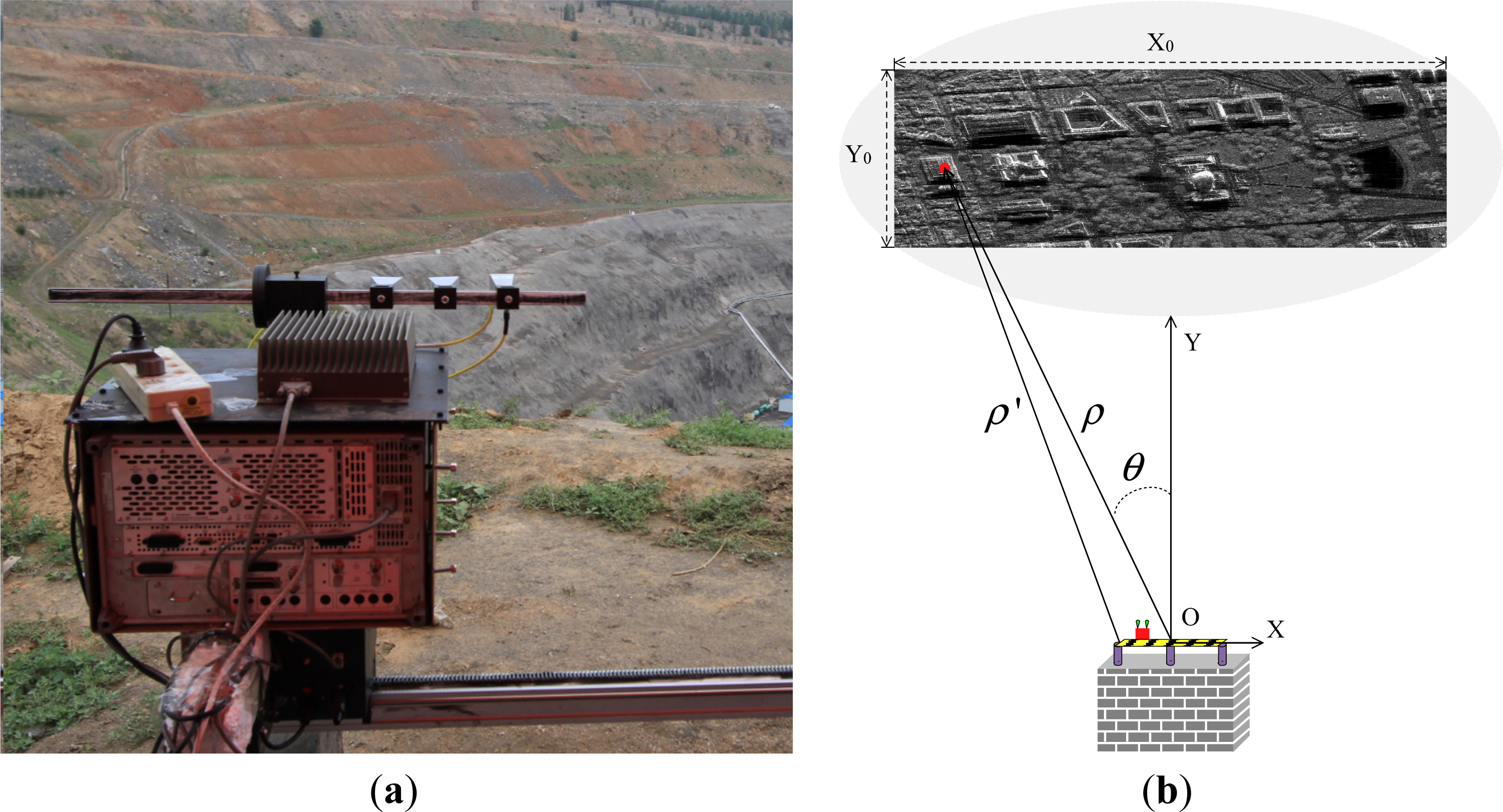
As can be seen in the first image of Figure 1, the airborne flies in an arbitrary path, the 2D image (range dimension and array dimension) can be obtained at any position of the flight path, much like pressing the shutter of a camera, as the transmitting-receiving time of the array radar is very short (for example, our system in built, 128 array channels, the transmitting-receiving time of every channel is 5 μs, the total transmitting-receiving time is 0.64 ms.). The autonomous navigation airborne forward-looking SAR imaging geometry in three dimensional coordinate at any position of the flight path can be seen in the second and third images in Figure 1. The top view of the autonomous navigation airborne forward-looking SAR imaging geometry can be seen in the last image in Figure 1.

The azimuth aperture of the autonomous navigation airborne forward-looking SAR is formulated with the cross-track dimensional linear array. The linear array can be densely or sparsely configured at the bottom of the airborne platform. X axis is the azimuth dimension, which is in parallel with the linear array. Y axis is the radar range dimension. O is the origin. Range dimensional resolution is obtained with wide band signal compression and azimuth dimensional resolution is obtained with physical array aperture synthesis. The length of the aperture is L and the size of the imaging area is X₀ in azimuth dimension and Y₀ in range dimension. For autonomous navigation airborne forward-looking SAR system circumstance, the length of the azimuth aperture is much shorter than the azimuth-imaging swath (X₀ ≪ L). The instantaneous range from the radar APC to the target P is ρ′. The reference range from the origin to the target P is ρ. The angle between the Y axis and OP is θ. The coordinate of the target, P, in the XOY coordinate is (ρsinθ, ρcosθ). The coordinate of the radar antenna phase center (APC) in the XOY coordinate is (x_n, 0).

The autonomous navigation airborne forward-looking SAR with linear array placed at the bottom of the platform is a multi-channel system. This multi-channel system usually works at a time-divided transmitting-receiving mode. The airborne platform movement during the time-divided transmitting-receiving procedure causes a Doppler shift to the echo signal. The Doppler shift effect can be compensated according to the method in [17] and [18]. The following echo signal model and imaging algorithm are all on the basis of the Doppler shift compensated.

3. Autonomous Navigation Airborne Forward-Looking SAR Echo Signal Model

In this section, the autonomous navigation airborne forward-looking SAR echo signal model is discussed. A chirp signal with carrier frequency f_c, chirp rate K_r, and pulse width T_P is transmitted and received. The transmitted signal can be written as [1]:

$$D(t)=\text{rect}(\frac{t}{T_p})\times \text{exp}\{\text{j}[2\pi f_c\hspace{0.17em}\text{t}+\pi K_r{t}^2]\}$$

(1)

where t is the fast time. Here, we are going to develop an equation for the signal phase received by the airborne forward-looking SAR system for the scatter object, P, at the coordinate (ρsinθ, ρcosθ). This development assumes an ideal point scatter object with a radar cross section, σ, of which the amplitude and phase characters do not vary with frequency and aspect angle [1]. For simplicity, the receiving signal model ignores antenna gain, amplitude effects of propagation on the signal, and any additional time delays due to atmospheric effects [1]. The signal received from the target, P, at azimuth sample x_n is:

$$D_r(x_n,\hspace{0.17em}\text{t})=a_t\times \text{rect}(\frac{t-t_d}{T_p})\times \text{exp}\{\text{j}[2\pi \hspace{0.17em}{f}_c(t-t_d)+\pi K_r{(t-t_d)}^2]\}$$

(2)

where ${\mathit{a}}_{\mathit{t}}=\sqrt{\mathit{\sigma }}$, ${\mathit{t}}_{\mathit{d}}=\frac{\mathbf{2}{\mathit{\rho }}^{\mathbf{\prime }}}{\mathit{c}}$ is the dual time delay from the radar APC to the target P. The radar-recorded signal is the video frequency signal generated by mixing the received signal with the carrier frequency signal. It is convenient to write the video frequency echo signal in the form:

$$D_r(x_n,\text{t})=a_t\times \text{rect}(\frac{t-t_d}{T_p})\times \text{exp}\{\text{j}[-2\pi \hspace{0.17em}{\mathit{ft}}_d+\pi K_r{(t-t_d)}^2]\}$$

(3)

Range frequency domain echo signal can be obtained by performing range FFT. The obtained range frequency domain signal can be written as:

$$D_r(x_n,f_m)=a_t\times \text{exp}\{-\text{j}\frac{4\pi (f_c+f_m)}{c}{\rho }^{\prime }\}\times D(f_m)$$

(4)

where D(f_m) is the frequency domain transmitted chirp signal, f_c is the carrier frequency term, f_m is the baseband frequency term, ${\mathit{f}}_{\mathit{m}}\mathbf{\in }[-\frac{{\mathit{f}}_{\mathit{s}}}{\mathbf{2}}\mathbf{,}\frac{{\mathit{f}}_{\mathit{s}}}{\mathbf{2}}]$, and f_s is the sampling frequency (f_s = 1.1∼1.3 B_r, typically f_s =1.2B_r). The range frequency matched filtered signal can be written as:

$$D_r(x_n,f_m)=a_t\times \text{exp}\{-\text{j}\frac{4\pi (f_c+f_m)}{c}{\rho }^{\prime }\}\times D(f_m)\times D^H(f_m)=a_t\times \text{exp}\{-\text{j}\frac{4\pi (f_c+f_m)}{c}{\rho }^{\prime }\}$$

(5)

where D^H(f_m) is the complex conjugate of the frequency domain transmitted chirp signal. ρ′ is the range from the radar APC (x_n, 0) to the target P at (ρsinθ, ρcosθ). Based on the range course Fresnel approximation, the echo signal received from target P can be written as:

$$\begin{array}{l}{D}_r(x_n,f_m)=a_t\times \text{exp}\{-\text{j}\frac{4\pi (f_c+f_m)}{c}\sqrt{{(x_n-\rho \hspace{0.17em}\text{sin}\hspace{0.17em}\theta )}^2+{(\rho \hspace{0.17em}\text{cos}\hspace{0.17em}\theta )}^2}\}\\ \approx a_t\times \text{exp}\{-\text{j}\frac{4\pi (f_c+f_m)}{c}(\rho -x_n\hspace{0.17em}\text{sin}\hspace{0.17em}\theta +\frac{x_n^2\hspace{0.17em}{\text{cos}}^2\hspace{0.17em}\theta }{2\rho })\}\end{array}$$

(6)

4. High Precision Imaging with Combination of Pseudo-Polar Formatting and Overlapped Sub-Aperture Algorithm

According to the echo model in Equation (6), the radar reflectivity at the point P can be estimated as follows:

$$a_t=\sum _{n=0}^{N-1}\sum _{m=0}^{M-1}{D}_r(x_n,f_m)\times \text{exp}\{\text{j}\frac{4\pi (f_c+f_m)}{c}\hspace{0.17em}(\rho -x_n\hspace{0.17em}\text{sin}\hspace{0.17em}\theta +\frac{x_n^2\hspace{0.17em}{\text{cos}}^2\hspace{0.17em}\theta }{2\rho })\}$$

(7)

With azimuth pseudo-polar formatting according to the relationship (f_c + f_m)x_n = f_cx′_n, the radar reflectivity at the point P can be written as:

$$a_t=\sum _{n=0}^{N-1}\sum _{m=0}^{M-1}{D}_r({x^{\prime }}_n,f_m)\times \text{exp}\{\text{j}(f_m\alpha -{x^{\prime }}_n\beta )\}\times \text{exp}\{\text{j}\eta {x^{\prime }}_n^2({(\frac{4\pi }{\lambda })}^2-{\beta }^2)\}$$

(8)

where $\alpha =\frac{4\pi \rho }{c}$, $\beta =\frac{4\pi \mathit{sin}\theta }{\lambda }$, $\eta =\frac{\lambda }{8\pi \rho }$, λ is the wavelength. The first exponent term is the linear phase term used for imaging, the second exponent term is the wave front curvature phase error term. The wave front curvature phase error term needs to be compensated for in order to avoid defocus and distortion, e.g., the targets appear defocused and located at false locations. Then the reconstructed image is sampled in (α, β) pseudo-polar format coordinate where α corresponds to the range dimension, β corresponds to the azimuth dimension [16]. α dimensional imagery with FFT can be written as:

$$a_t=\text{sinc}(\frac{B\alpha }{2\pi })\times \sum _{n=0}^{N-1}D({x^{\prime }}_n,\alpha )\times \text{exp}\{-\text{j}{x^{\prime }}_n\beta \}\times \text{exp}\{\text{j}\eta {x^{\prime }}_n^2({(\frac{4\pi }{\lambda })}^2-{\beta }^2)\}$$

(9)

where D(x′_n, α) is the range compressed signal. The ρ and θ intervals, where the image shall be free of any ambiguities [16], are defined as follows:

$$\{\begin{array}{c}0\le \rho \le \frac{c}{2\Delta f}\\ -\text{arcsin}(\frac{\lambda }{4\Delta x^{\prime }})\le \theta \le \text{arcsin}(\frac{\lambda }{4\Delta x^{\prime }})\end{array}$$

(10)

where Δf is the range frequency sample interval, and Δx′ is the azimuth sample interval after pseudo-polar formatting.

The wave front curvature phase error term defocuses the reconstructed image, if we require the azimuth defocus effect to be less than β resolution, the second exponent term should satisfy:

$${\frac{\partial \left(\eta \cdot {x_n^{\prime }}^2\left({\left(\frac{4\pi }{\lambda }\right)}^2-{\beta }^2\right)\right)}{\partial x_n^{\prime }}|}_{x_n^{\prime }=\frac{L}{2},\theta =0}<\frac{2\pi }{L}$$

(11)

Take maximum β according to Equation (10) into Equation (11), we obtain:

$$\rho >\frac{L^2}{\lambda }$$

(12)

According to Equation (12), the relationship among the minimum range ρ, the azimuth aperture L and the wavelength λ is shown in Figure 2, where, the azimuth aperture L ∈[0.8, 3] m and the wavelength λ ∈ [0.008, 0.03] m. The defocus and distortion effects caused by the wave front curvature phase error term selects Ku band (center frequency 17.25 GHz) and can be seen in Figure 3 (demonstration). The imaging scene size used in the demonstration is, range: 400 m∼600 m, azimuth: −100 m∼100 m. Figure 3a is the ideal image formation plane in 3D view (range, azimuth and elevation) without defocus and distortion effects. Figure 3b is the ideal image formation plane in 2D projection view (range and azimuth) without defocus and distortion effects. Figure 3c is the image formation plane in 3D view (range, azimuth and elevation) with defocus and distortion effects. Figure 3d is the image formation plane in 2D projection view (range and azimuth) with defocus and distortion effects.

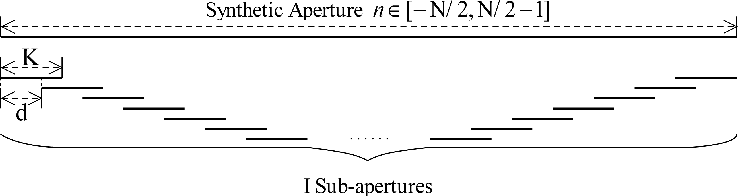
In autonomous navigation airborne forward-looking SAR circumstance, the condition in Equation (11) and Equation (12) is usually not satisfied. In this section, we perform β dimension high precision imaging with an overlapped sub-aperture algorithm in order to compensate the wave front curvature phase error. The azimuth synthetic aperture is composed of N azimuth samples. We divide the azimuth synthetic aperture into I sub-apertures, each sub-aperture consists of K samples, and there are K-d overlapped samples between the adjacent sub-apertures [19–21]. The sub-aperture division is illustrated in Figure 4.

Suppose the azimuth spacing interval is Δx′ after pseudo-polar formatting, which means, x′_n = n × Δx′, where $\mathbf{n}\mathbf{\in }[\mathbf{-}\frac{\mathit{N}}{\mathbf{2}}\mathbf{,}\frac{\mathit{N}\mathbf{-}\mathbf{1}}{\mathbf{2}}]$. With sub-aperture division, x′_n = (i × d + k) Δx′, where $\mathbf{i}\mathbf{\in }[-\frac{\mathit{I}}{\mathbf{2}}\mathbf{,}\frac{\mathit{I}\mathbf{-}\mathbf{1}}{\mathbf{2}}]$ and $\mathbf{n}\mathbf{\in }[-\frac{\mathit{N}}{\mathbf{2}}\mathbf{,}\frac{\mathit{N}-\mathbf{1}}{\mathbf{2}}]$. I, K, and N are all even numbers. Take the sub-aperture term into Equation (9), and we obtain:

$$\begin{array}{l}{a}_t=\text{sinc}(\frac{B\alpha }{2\pi })\times \sum _{i=0}^{I-1}\sum _{k=0}^{K-1}D(i,k,\alpha )\times \text{exp}\{-\text{j}id\Delta x^{\prime }\beta +\text{j}\eta i^2{d}^2\hspace{0.17em}{x_n^{\prime }}^2({(\frac{4\pi }{\lambda })}^2-{\beta }^2)\}\times \\ \text{exp}\{-\text{j}k\Delta x^{\prime }\beta +2\text{j}\eta idk{x_n^{\prime }}^2({(\frac{4\pi }{\lambda })}^2-{\beta }^2)\}\times \text{exp}\{\text{j}\eta k^2\hspace{0.17em}{x_n^{\prime }}^2({(\frac{4\pi }{\lambda })}^2-{\beta }^2)\}\end{array}$$

(13)

where D(i, k, α) is the range compressed signal in an azimuth matrix in the form of variables i and k. The maximum instantaneous wave front phase error caused by the second exponent term can be ignored if:

$${\frac{\partial (2\text{j}\eta idk{x_n^{\prime }}^2({(\frac{4\pi }{\lambda })}^2-{\beta }^2)+\eta k^2\hspace{0.17em}{x_n^{\prime }}^2({(\frac{4\pi }{\lambda })}^2-{\beta }^2))}{\partial k}|}_{k=\frac{K}{2},i=\frac{I}{2},\theta =0}<\frac{2\pi }{K\Delta x^{\prime }}$$

(14)

In autonomous navigation airborne forward-looking SAR circumstance, the condition in Equation (14) is usually satisfied as K is much smaller than N. According to Equation 14, if we ignore the wave front curvature phase error caused by the second exponent term, and perform IFFT along the k dimension, we obtain:

$$a_t=\text{sinc}(\frac{B\alpha }{2\pi })\times \text{sinc}(\frac{K}{2}(\Delta x^{\prime }\beta -\frac{2\pi k}{K}))\times \sum _{i=0}^{I-1}D(i,k,\alpha )\times \text{exp}\{-\text{j}id\Delta x^{\prime }\beta +j\eta i^2{d}^2\hspace{0.17em}{x_n^{\prime }}^2({(\frac{4\pi }{\lambda })}^2-{\beta }^2)\}$$

(15)

Then β can be estimated as $\overline{\beta }=\frac{2\pi k}{K\Delta x^{\prime }}$. Then the wave front curvature phase error compensation term g(i) along the i dimension can be written as:

$$g(\text{i})=\text{exp}\{\text{j}id\Delta x^{\prime }\overline{\beta }-\text{j}\eta i^2{d}^2\hspace{0.17em}{x_n^{\prime }}^2({(\frac{4\pi }{\lambda })}^2-{\overline{\beta }}^2)\}$$

(16)

The phase compensation term g(i) is applied to compensate the exponent term in Equation (15). The wave front phase error compensated result can be written as:

$$a_t=\text{sinc}(\frac{B\alpha }{2\pi })\times \text{sinc}(\frac{K}{2}(\Delta x^{\prime }\beta -\frac{2\pi k}{K}))\times \sum _{i=0}^{I-1}D(i,k,\alpha )\times \text{exp}\{-\text{j}id\Delta x^{\prime }(\beta -\overline{\beta })+j\eta i^2\hspace{0.17em}{d}^2\hspace{0.17em}{x_n^{\prime }}^2({\beta }^2-{\overline{\beta }}^2)\}$$

(17)

We perform IFFT along the i dimension and obtain:

$$a_t=\text{sinc}(\frac{B\alpha }{2\pi })\times \text{sinc}(\frac{K}{2}(\Delta x^{\prime }\beta -\frac{2\pi k}{K}))\times \text{sinc}(\frac{I}{2}(\Delta x^{\prime }(\beta -\overline{\beta })-\frac{2\pi i}{I}))$$

(18)

We transform the azimuth image from matrix sample (i, k) to vector sample, n, according to the relationship in Figure 4. The azimuth high precision imaging is finished until here. The flow diagram of autonomous navigation airborne forward-looking SAR pseudo-polar formatting overlapped sub-aperture algorithm is illustrated in Figure 5.

An important advantage of the proposed pseudo-polar formatting and overlapped sub-aperture algorithm is that the resulting image shows an invariant resolution within the entire image scene. The resolution in pseudo-polar image is $\Delta \alpha =\frac{0.89}{B_r}$ and $\Delta \beta =\frac{0.89}{L}$, respectively [16]. The azimuth resolution in pseudo-polar coordinate separates the image azimuth pixel in angle θ ( $\beta =\frac{4\pi \text{sin}\theta }{\lambda }$). The invariant resolution condition is not satisfied in Cartesian image, where the azimuth resolution is a function of wavelength λ, range ρ, angle θ, and the aperture length L in the form of $\Delta y=\frac{\lambda \rho }{2L\text{cos}\theta }$ [22]. The azimuth resolution in the Cartesian coordinate separates the image azimuth pixel in distance, not the angle. Consequently, it is a good practice to use the pseudo-polar coordinate image at all the stages of the processing chain but the last one, where we have to geolocate the image.

5. Imaging Results with Real Data

The Ground Based SAR (GBSAR) system is widely used for slope area and glacier deformation monitoring for its low de-correlation compared with space-borne data [23–27]. Fortunately, the Ground Based SAR (GBSAR) system possesses the same imaging geometry with the airborne forward-looking SAR. In order to verify the proposed autonomous navigation airborne forward-looking SAR high precision imaging algorithm, we perform a Ku band GBSAR experiment. The measurement parameters of the experiment we used are described in

Table 1. Measurement parameters used in the experiment.

Measurement Parameters	Value
Carrier Frequency	17.25 GHz
Bandwidth	500 MHz
Range Sample Number	4001
Azimuth Synthetic Aperture	2.56 m
Azimuth Sample Interval	0.01 m
Azimuth Sample Number	256

.

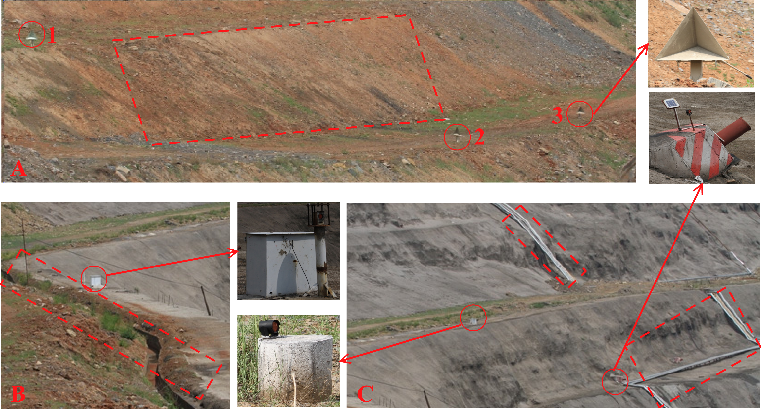
The sketch view of the observed imaging scene is shown in Figure 6a. The radar is placed on the opposite of a slope area. The GBSAR imaging geometry is shown in Figure 6b, which is the same as autonomous navigation airborne forward-looking SAR (short azimuth aperture, wide azimuth swath). The strong scatterer in the imaging scene is shown in Figure 7, including trihedral angle reflector, metal box, concrete stone, and metal pipe lines. The imaging scene is located in the range of 200 m–800 m. 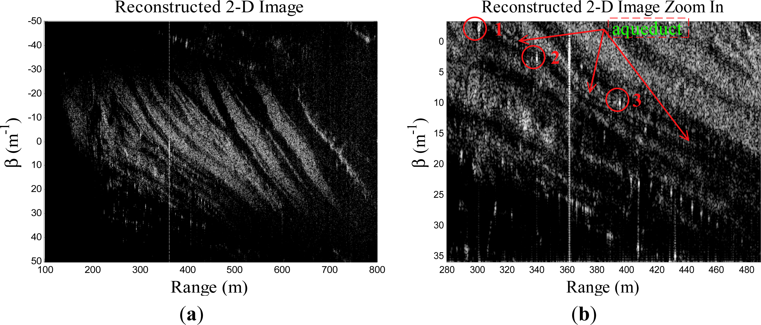According to Equation (12), the condition ρ ≥ 370m should be satisfied in order to ignore the wave front phase error term. The reconstructed image with range matched filtering, and pseudo-polar formatting (no overlapped sub-aperture processing is operated), is shown in Figure 8a. The zoomed area of the water channel and pipe lines is shown in Figure 8b.

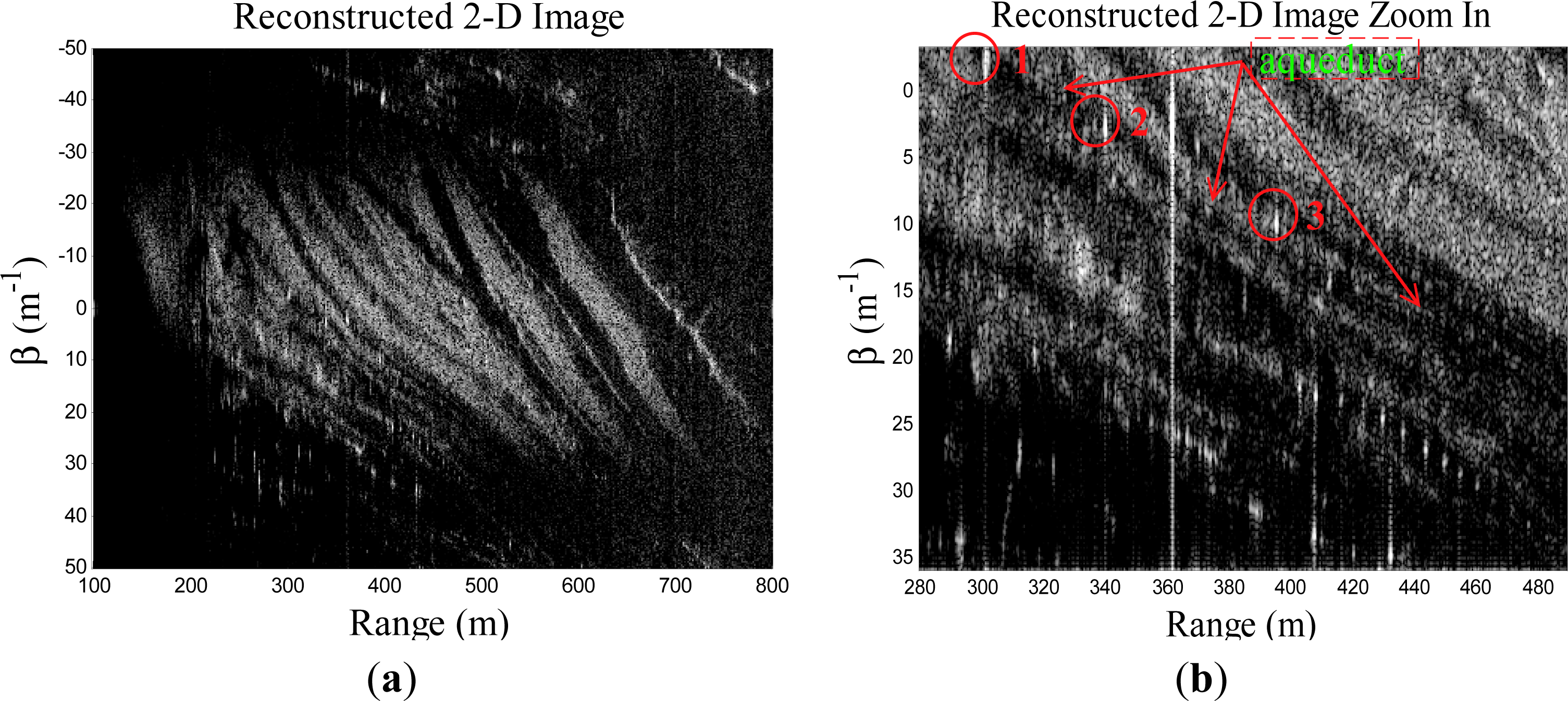
In order to obtain a high precision imaging result, the image reconstruction is operated with the proposed combination of pseudo-polar formatting and an overlapped sub-aperture algorithm. The azimuth synthetic aperture (256 azimuth samples) is divided into 30 overlapped sub-apertures, every sub-aperture contains 16 azimuth samples, and every two adjacent sub-apertures contain eight overlapped azimuth samples. The reconstructed image with the proposed algorithm is shown in Figure 9a. The zoomed area of the water channel and pipe lines is shown in Figure 9b.

By comparing the reconstructed images in Figures 8 and 9, we notice that the reconstructed image with the proposed method is much more precise. The aqueduct is very clear in Figure 9b while it is very blurry in Figure 8b. Detail information, better contrast, and better dynamic range can be obtained in high precision reconstructed images. This information is very important for image understanding. The pilot can make more precise judgments with a high precision reconstructed image [10].

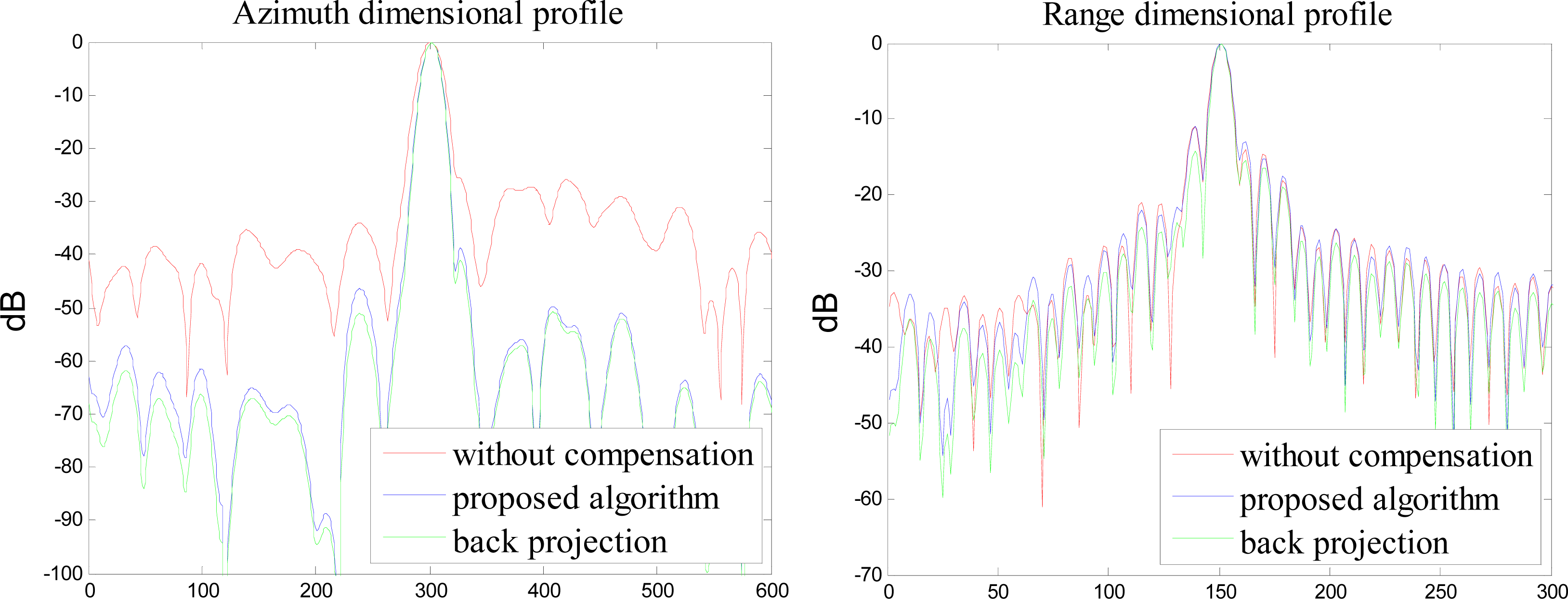
In order to clarify the performance of the proposed imaging algorithm, we compare the range and azimuth dimensional profile response of the trihedral angle reflectors placed in the imaging scene reconstructed with the proposed imaging algorithm and back projection algorithm. The range and azimuth profile response of the trihedral angle reflectors labeled 1, 2, and 3 in the imaging scene is shown in Figures 10 and 12, respectively. As can be seen from Figures 10 and 12, the red line is the profile response of the trihedral angle reflectors reconstructed with the pseudo polar format method, without wave front curvature phase error compensation, the blue line is the profile response of the trihedral angle reflectors reconstructed with the proposed pseudo polar formatting and overlapped sub-aperture algorithm, and the green line is the profile response of the trihedral angle reflectors reconstructed with the back projection algorithm. It is obvious that when reconstructed with different methods, the azimuth profile response is different. The side lobe is very high in the azimuth profile response when reconstructed with the pseudo polar format method, without wave front curvature phase error compensation. The azimuth profile response reconstructed with the back projection algorithm is the most outstanding, while the computation efficiency of back projection algorithm is very low. The azimuth profile response, reconstructed with the proposed polar formatting and overlapped sub-aperture algorithm, is almost the same as that of back projection algorithm, while the computation efficiency is much better.

As is illustrated in the last part of Section 4, the reconstructed image in the pseudo-polar coordinate owns the same invariant azimuth resolution, which means that the main lobe of the trihedral angle reflectors’ azimuth profile is the same. The reconstructed image in the Cartesian coordinate owns variant azimuth resolution, which means the main lobe of the trihedral angle reflectors’ azimuth profile is different. From the imaging result shown in Figure 9b, the position of the trihedral angle reflectors labeled 1, 2, and 3 are (−1.9°, 301.2 m), (2.7°, 340 m), and (9.9°, 393.4 m).

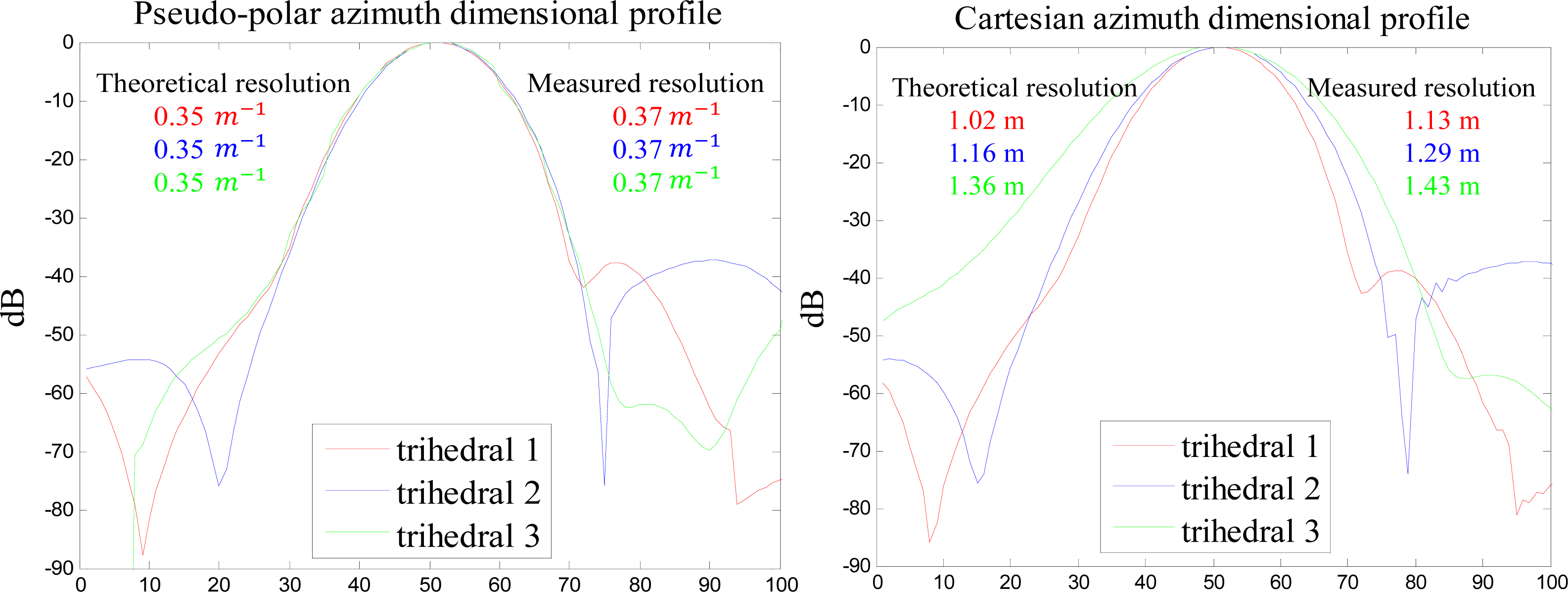
In order to clarify the pseudo-polar and Cartesian coordinate azimuth response, we compare the azimuth resolution of the trihedral angle reflector in the pseudo-polar and Cartesian coordinate, which is shown in Figure 13. The left image of Figure 13 is the pseudo-polar azimuth dimensional profile of three different trihedral angle reflectors. The main lobe of the azimuth response, theoretical resolution, and measured resolution of the trihedral angle reflector labeled 1, 2, and 3 are displayed in red, blue, and green. It is obvious that the main lobe of the different trihedral angle reflectors is almost the same, which means the azimuth resolution is invariant in the pseudo-polar coordinate image. The right image of Figure 13 is the Cartesian azimuth dimensional profile of three different trihedral angle reflectors. The main lobe of the azimuth response, theoretical resolution, and measured resolution of the trihedral angle reflector labeled 1, 2, and 3 are displayed in red, blue, and green. It is obvious that the main lobes of different trihedral angle reflectors are different. The main lobe of the trihedral angle reflector 1 is sharper than that of the trihedral angle reflector 2, the main lobe of the trihedral angle reflector 2 is sharper than that of the trihedral angle reflector 3, which means the azimuth resolution of the trihedral angle reflector 1 is better than that of trihedral angle reflector 2, and the azimuth resolution of the trihedral angle reflector 2 is better than that of trihedral angle reflector 3. This azimuth resolution tendency is in accordance with theoretical computation and realistic measurement. The pseudo-polar image, or the Cartesian image, has a common point: the theoretical resolution and the measured resolution is almost the same (the minor difference is caused by radar antenna pattern influence, noise, etc.).

We conclude with some minor suggestions regarding the practical use of this technique. The authors have implemented and extensively tested the proposed high precision imaging method with GBSAR experiments using Matlab (the Mathworks, MA, USA) and C/C++. The main computation operations in this algorithm include FFT/IFFT, complex matrix multiplication, and interpolation. Then high precision imaging result can be obtained in real time with parallel implementation. According to our experiences, the elapsed time for image reconstruction with the measurement parameters in the simulation is 0.3 second at Intel(R) Core(TM) i7 2600@3.40 GHz CPU platform.

6. Conclusions

Autonomous navigation airborne forward-looking synthetic aperture radar (SAR) observes the anterior inferior wide area with a short cross-track dimensional linear array as azimuth aperture. The short azimuth aperture wide azimuth swath application scenario is drastically different from that of side-looking space-borne, or air-borne, SAR system. The imaging geometry, echo signal model, and pseudo-polar formatting, and overlapped sub-aperture algorithm for autonomous navigation airborne forward-looking SAR imaging are illustrated. The range dimensional imaging is operated with wide band signal compression. The azimuth synthetic aperture is divided into several overlapped sub-apertures. Intra sub-aperture IFFT, wave front curvature phase error compensation, and inter sub-aperture IFFT is operated sequentially to finish azimuth high precision imaging. We demonstrate outdoor GBSAR experiments that possess the same imaging geometry as the airborne forward-looking SAR to validate the effectiveness and performance of our proposed algorithm. We also compare and analyze the profile response of the trihedral angle reflectors placed in the imaging scene reconstructed with the proposed imaging algorithm and back projection algorithm. The proposed algorithm possesses the advantage of high reconstruction precision, low memory cost, and medium computation complexity.