Multi-Sensor Platform for Indoor Mobile Mapping: System Calibration and Using a Total Station for Indoor Applications


Abstract
:1. Introduction
2. Measurement System
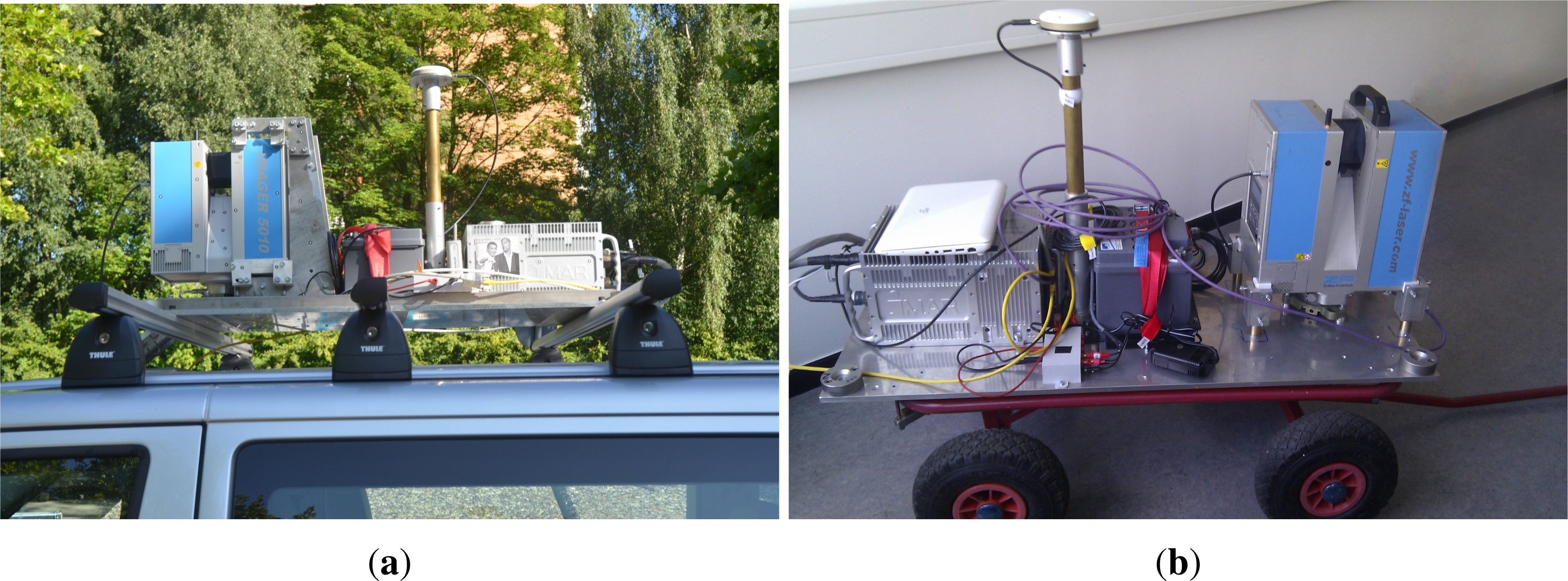
2.1. Outdoor
2.2. Indoors
3. Calibration
3.1. Estimation of the Accuracy
3.2. Internal Position and Orientation Determination
3.3. External Position and Orientation Determination
3.4. Field Procedure
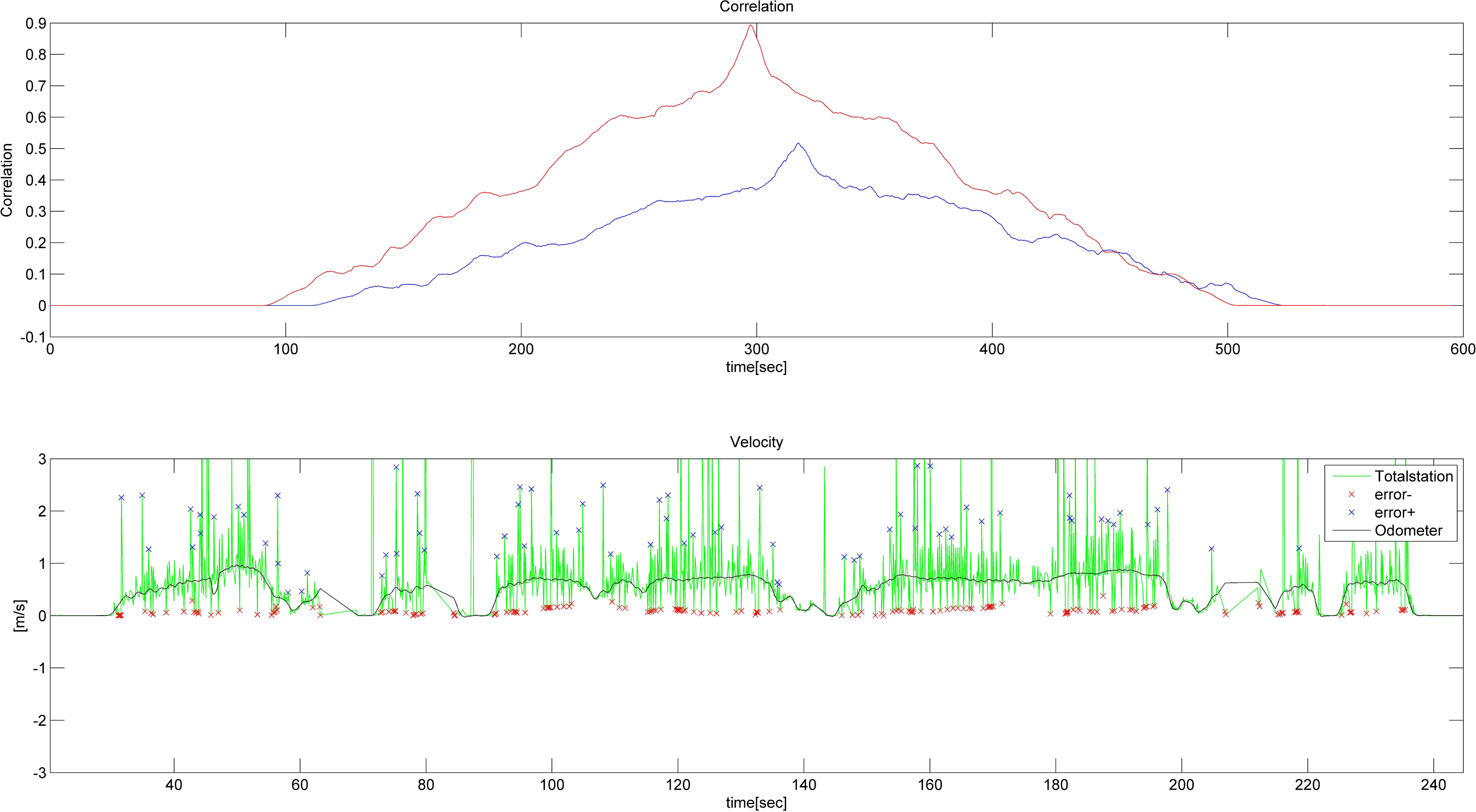
4. Total Station
5. Sensor Fusion
5.1. Prediction
5.2. Correction
5.3. Smoothing
6. Results and Discussion
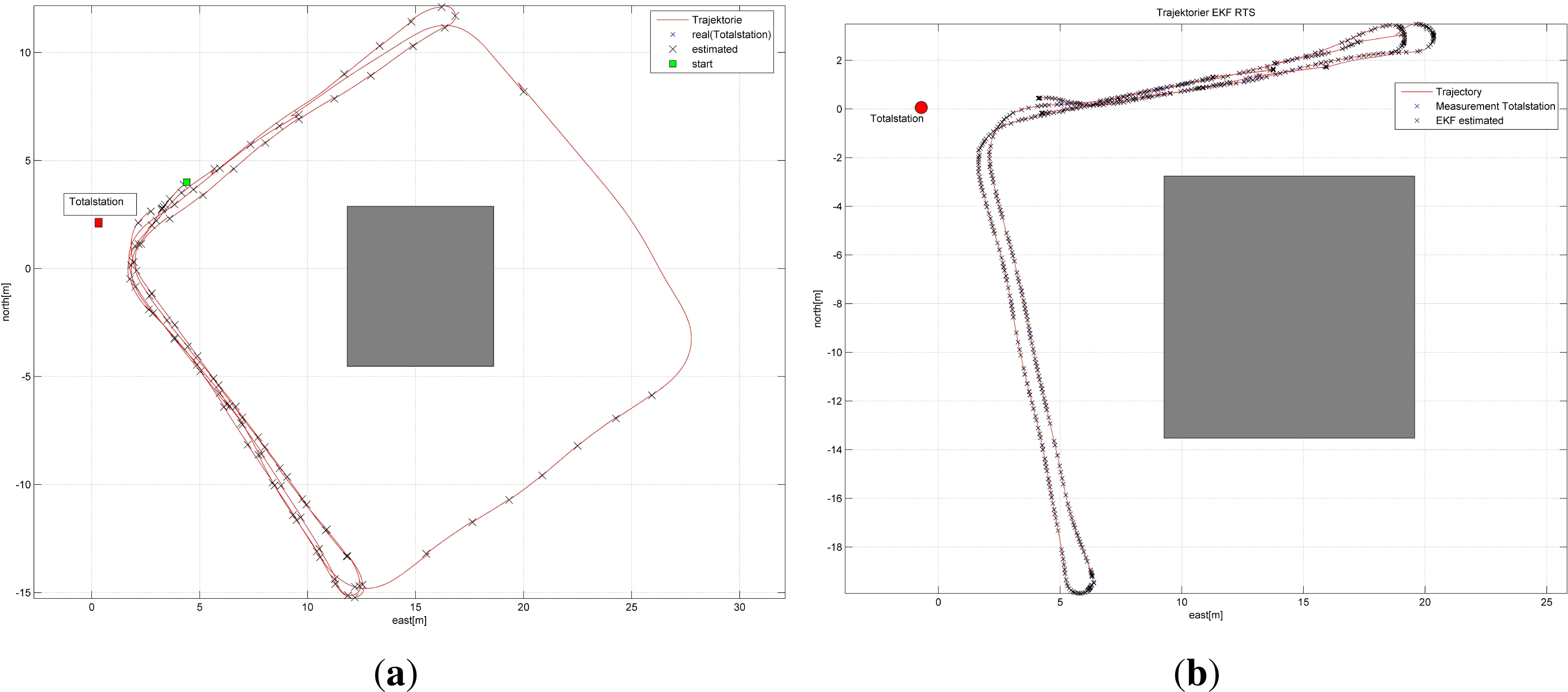
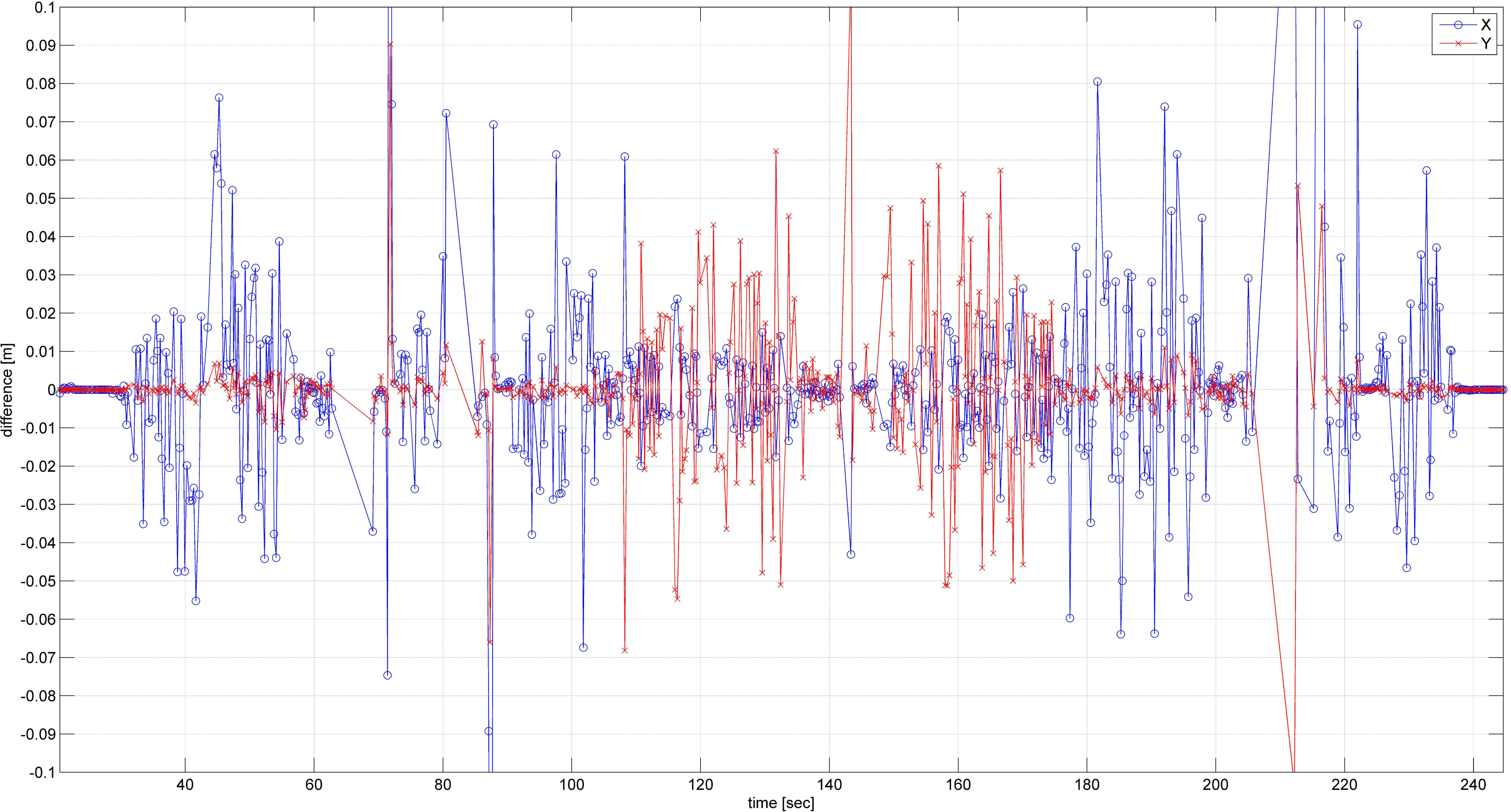
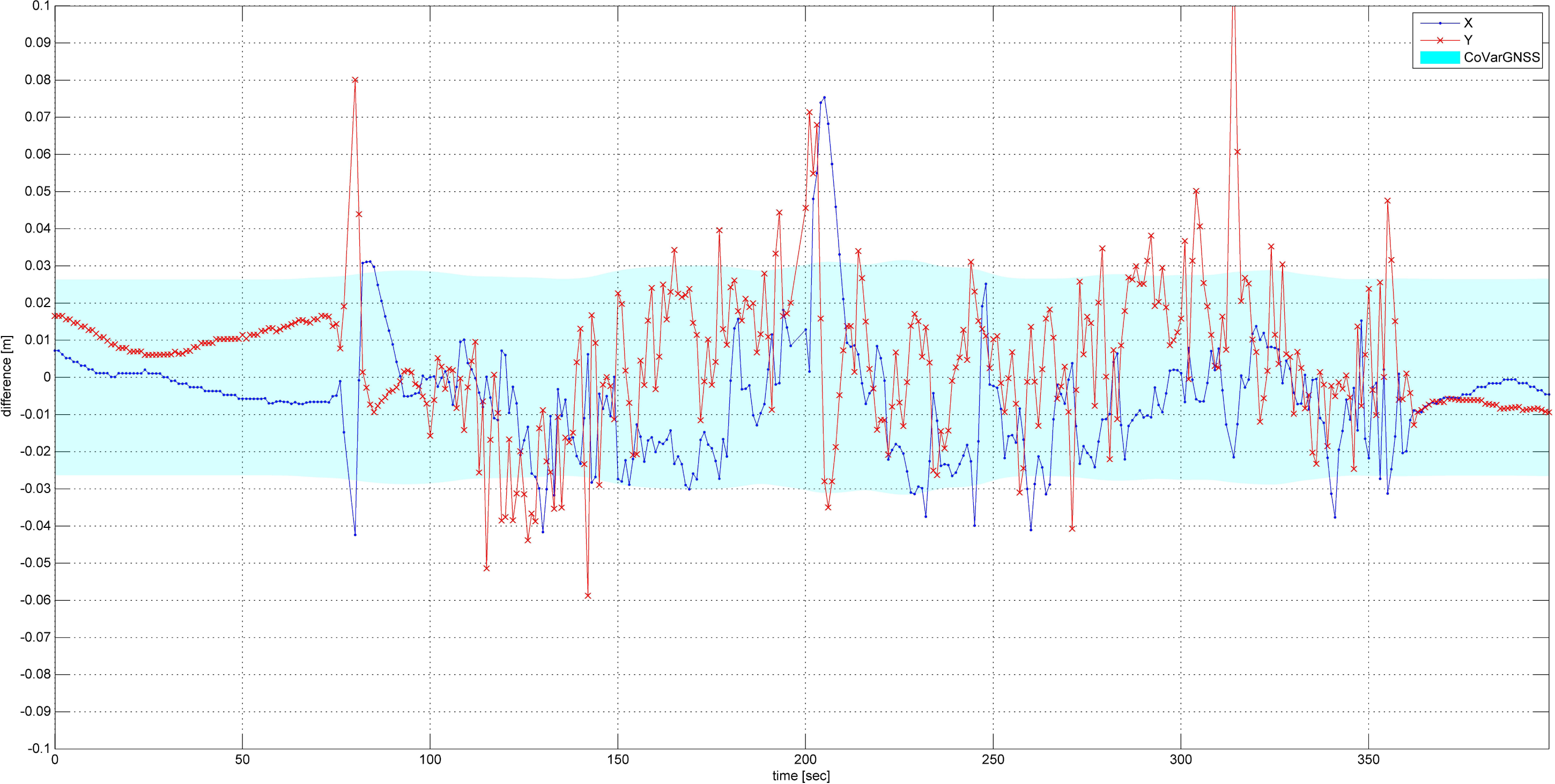
6.1. Outdoor Test
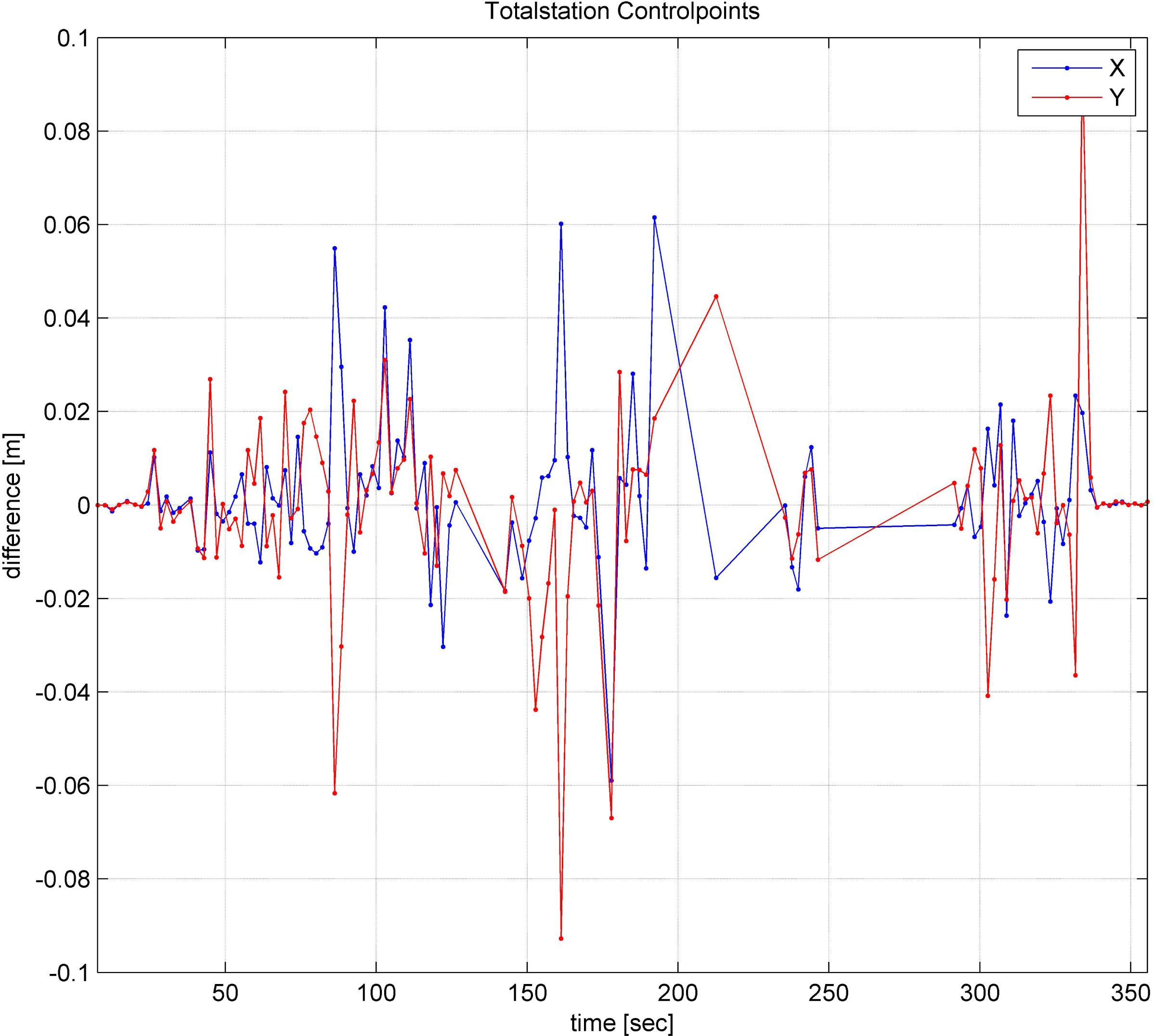
6.2. Indoor Test
- \%R1Q,2167
7. Conclusions
Conflict of Interest
References
- El-Sheimy, N. An Overview of Mobile Mapping Systems. Proceedings of the FIG Working Week 2005, Cairo, Egypt, 16–21 April 2005.
- Kaartinen, H.; Hyyppä, J.; Kukko, A.; Jaakkola, A.; Hyyppä, H. Benchmarking the performance of mobile laser scanning systems using a permanent test field. Sensors 2012, 12, 12814–12835. [Google Scholar]
- Brenner, C. Extraction of features from mobile laser scanning data for future driver assistance systems. Adv. GISci. 2009. [Google Scholar] [CrossRef]
- Haala, N.; Peter, M.; Kremer, J.; Hunter, G. Mobile LiDAR mapping for 3D point cloud collection in urban areas—A performance test. Int. Arch. Photogr. Remote Sens. Spat. Inf. Sci 2008, 37, 1119–1127. [Google Scholar]
- Hassan, T.; El-Sheimy, N. Common adjustment of land-based and airborne mobile mapping system data. Int. Arch. Photogramm. Remote Sens. Spat. Inf. Sci 2008, 37, 835–842. [Google Scholar]
- Puente, I.; González-Jorge, H.; Martínez-Sánchez, J.; Arias, P. Review of mobile mapping and surveying technologies. Measurement 2013, 46, 2127–2145. [Google Scholar]
- Petrie, G. An introduction to the technology mobile mapping systems. Geoinformatics 2010, 13, 32–42. [Google Scholar]
- Graham, L. Mobile mapping systems overview. Photogr. Eng. Remote Sens 2010, 76, 222–228. [Google Scholar]
- Graefe, G. Quality Management in Kinematic Laser Scanning Applications. Proceedings of the The 5th International Symposium on Mobile Mapping Technology (MMT’07), Padua, Italy, 29–31 May 2007.
- Schwarzenberger, J. Evaluierung und Kalibierung eines Mobile Mapping Systems. HafenCity Universität, Hamburg, Germany, 2013. [Google Scholar]
- International Hydrographic Organization (IHO). Chapter 3 Depth Determination. In Manual on Hydrography Publication C-13, 1st ed.; International Hydrograpic Organization, International Hydrographic Bureau: Monaco, China, 2011. [Google Scholar]
- Keller, F.; Sternberg, H. Kombination von Hydrographie und Terrestrischen Laserscannern-Systematische Effekte, Kalibrier- und Auswertemethoden. Proceedings of Bundesanstalt für Gewässerkunde: Kolloquium Neue Entwicklungen in der Gewässervermessung, Koblenz, Germany, 20–21 November 2012.
- Seube, N.; Picard, A.; Rondeau, M. A simple method to recover the latency time of tactical grade IMU systems. ISPRS J. Photogramm. Remote Sens 2012, 74, 85–89. [Google Scholar]
- Stempfhuber, W.; Schnaedelbach, K.; Maurer, W. Genaue Positionierung von bewegten Objekten mit Zielverfolgenden Tachymetern. Proceedings of the XIII International Course on Engineering Surveying (Ingenieurvermessung 2000), München, Germany, 13–17 March 2000.
- Kalman, R.E. A new approach to linear filtering and prediction problems. ASME J. Basic Eng 1960, 82, 35–45. [Google Scholar]
- Welch, G.; Bishop, G. An Introduction to the Kalman Filter; Technical Report 95-041; University of North Carolina Computer Science-Chapel Hill: Chapel Hill, NC, USA, 1995. [Google Scholar]
- Rauch, H.E.; Tung, F.; Striebel, C.T. Maximum likelihood estimates of linear dynamic systems. AIAA J 1965, 3, 1445–1450. [Google Scholar]
- Grewal, M.S.; Andrews, A.P. Kalman Filtering. In Theory and Practice Using MATLAB; Wiley: Hoboken, NJ, USA, 2008. [Google Scholar]
- Beetz, A. Separation of Control Quality and Measurement Accuracy for Guiding Control Tasks of an Indoor Construction Machine Simulator. Proceedings of International Conference on Indoor Positioning and Indoor Navigation (IPIN 2012), Sydney, Australia, 13–15 November 2012.
- Leica. Leica TPS1200+ Leica TS30/TM30 GeoCOM Reference Manual; Version 1.50; Leica Geosystems AG: Heerbrugg, Switzerland, 2009. [Google Scholar]


| Manufacturer | Name | Accuracy/Resolution |
|---|---|---|
| Inertial Measurement Systems | ||
| IMAR | RQH1003 | 0.003 |
| GNSS | ||
| Novatel Receiver | OEMV-2 | - |
| Leica | AT502 Dual-frequency antenna | - |
| Laserscanner | ||
| Zoller + Fröhlich | 5010 | 0.0004 deg/5 mm |
| Sick | LMC121 | 12 mm |
| Odometer | ||
| Wachendorff | WDG58B | 10,000 I/U |
| Peiseler | Kfz-2000 | 2,000 I/U |
| Total station | ||
| Leica | TPS1201+ | 0.15 mgon/3 mm + 1.5 ppm |
| Camera | ||
| Point Grey | 2x Flea3 stereo | 1.4 MPixel |
| IMU only (m) | with Odometry (m) | with Total Station (m) | vs. GPS | |
|---|---|---|---|---|
| Maximum | 1.8049 | 1.0395 | 0.1105 | 0.1274 |
| Median | 0.5820 | 0.3783 | 0.0101 | 0.0164 |
| Mean | 0.7218 | 0.4140 | 0.0159 | 0.0202 |
| Std. | 0.4872 | 0.3268 | 0.0197 | 0.0149 |
| All (m) | Adjusted (m) | |
|---|---|---|
| Maximum | 0.5719 | 0.0958 |
| Median | 0.0101 | 0.0098 |
| Mean | 0.0186 | 0.0157 |
| Std. | 0.0410 | 0.0174 |
© 2013 by the authors; licensee MDPI, Basel, Switzerland This article is an open access article distributed under the terms and conditions of the Creative Commons Attribution license ( http://creativecommons.org/licenses/by/3.0/).
Share and Cite
Keller, F.; Sternberg, H. Multi-Sensor Platform for Indoor Mobile Mapping: System Calibration and Using a Total Station for Indoor Applications. Remote Sens. 2013, 5, 5805-5824. https://doi.org/10.3390/rs5115805
Keller F, Sternberg H. Multi-Sensor Platform for Indoor Mobile Mapping: System Calibration and Using a Total Station for Indoor Applications. Remote Sensing. 2013; 5(11):5805-5824. https://doi.org/10.3390/rs5115805
Chicago/Turabian StyleKeller, Friedrich, and Harald Sternberg. 2013. "Multi-Sensor Platform for Indoor Mobile Mapping: System Calibration and Using a Total Station for Indoor Applications" Remote Sensing 5, no. 11: 5805-5824. https://doi.org/10.3390/rs5115805
APA StyleKeller, F., & Sternberg, H. (2013). Multi-Sensor Platform for Indoor Mobile Mapping: System Calibration and Using a Total Station for Indoor Applications. Remote Sensing, 5(11), 5805-5824. https://doi.org/10.3390/rs5115805