Article

Assimilation of MODIS Snow Cover Area Data in a Distributed Hydrological Model Using the Particle Filter

Institute for Environment and Sustainability, European Commission, Joint Research Centre, I-21027 Ispra, Italy
*
Author to whom correspondence should be addressed.
Current Address: Hydrosystems and Bioprocesses Research Unit (HBAN), Irstea, 1, rue Pierre-Gilles de Gennes, CS 10030, 92761 Antony Cedex, France
Remote Sens. 2013, 5(11), 5825-5850; https://doi.org/10.3390/rs5115825
Submission received: 29 August 2013 / Revised: 23 October 2013 / Accepted: 24 October 2013 / Published: 8 November 2013
(This article belongs to the Special Issue Hydrological Remote Sensing)

Abstract

:
Snow is an important component of the water cycle, and its estimation in hydrological models is of great significance concerning the simulation and forecasting of flood events due to snow-melt. The assimilation of Snow Cover Area (SCA) in physical distributed hydrological models is a possible source of improvement of snowmelt-related floods. In this study, the assimilation in the LISFLOOD model of the MODIS sensor SCA has been evaluated, in order to improve the streamflow simulations of the model. This work is realized with the final scope of improving the European Flood Awareness System (EFAS) pan-European flood forecasts in the future. For this purpose daily 500 m resolution MODIS satellite SCA data have been used. Tests were performed in the Morava basin, a tributary of the Danube, for three years. The particle filter method has been chosen for assimilating the MODIS SCA data with different frequencies. Synthetic experiments were first performed to validate the assimilation schemes, before assimilating MODIS SCA data. Results of the synthetic experiments could improve modelled SCA and discharges in all cases. The assimilation of MODIS SCA data with the particle filter shows a net improvement of SCA. The Nash of resulting discharge is consequently increased in many cases.

1. Introduction

Snow is an important component of the water cycle and of the climate evolution [1]. Snowpacks can contain a huge quantity of water that can be released suddenly during the spring. Moreover, its characteristics, like the albedo, can have an important impact on surface energy fluxes. Research in recent years has been aimed at a better understanding of snowpack evolution and its simulation (e.g., [24]). However further investigation is needed in particular with respect to incorporating this information into hydrologic and Land Surface Models (LSMs, e.g., [5,6]). The assimilation of observed data in order to keep physical states of the models up-to-date, is a widely used technique in meteorology (e.g., [79]). Only in recent years its use in hydrology, for improving initial states and thus the simulation of flows, water budget, or snow pack, has significantly increased (e.g., [1014]).
Snow height observations are available from many meteorological stations. Unfortunately these data are very dependent on local conditions (wind, vegetation, slope, sun exposition) and are therefore only of limited use in large scale hydrological modeling. Moreover, they cannot represent the spatial variability of snow cover to a sufficiently accurate extent. Therefore the use of satellite observations of snow becomes an increasingly interesting alternative especially when simulating hydrologic processes in large-scale river basin models (e.g., [6,1521]). Such observations are usually available on a daily time-step and can cover large areas such as Europe or even the entire globe.
Snow satellite observations are found in two forms: Snow Water Equivalent (SWE), or Snow Cover Area (SCA). The quality of SWE data is often not high enough for use in hydrology, as studies have found large errors in microwave estimates compared with actual measurements because they are too much impacted by the forest cover, topography, snow type and are considered not reliable for high latitude tundra regions [16,22,23], and the data frequency is often low (most of the time around a week). There are two types of satellite SCA data: those derived from passive microwave sensors, or those from optical sensors. A major difference between these two types of data is that optical sensors cannot see through clouds, whereas for passive microwave sensors, clouds are not an issue. However, the sensors using passive microwaves, such as AMSR-E (Advanced Microwave Scanning Radiometer-EOS) or SSM/I (Special Sensor Microwave/Imager), provide data at a coarse resolution (more than 5 km for AMSR-E and more than 2.5 km for SSM/I) and with a lower frequency (more than a day), which limits its applicability to assimilation in models. The resolution of some radar data, such as RADARSAT or ASAR (Advanced Synthetic Aperture Radar), is very high, but the frequency of acquisition and the quality of observations seem not yet to reach the standards (daily frequency) needed for frequent assimilation in a hydrological model.
On the other hand, optical SCA data are more easily available for large areas and at a relatively high-sampling frequency, usually with good quality [24]. As a result, its use in hydrologic modeling has been increasing in recent years [15]. SCA gives information about the presence or not of snow on the surface, according to the satellite image. No indication about the snow quantity (height or SWE) can be given directly by SCA data. One direct drawback of the use of optical satellite-based SCA is the lack of penetration through clouds, which means that during some periods, a large amount of data can be lacking.The MODIS (Moderate Resolution Imaging Spectroradiometer) snow product, which is the satellite-based snow product that is the most widely used in hydrology, may contain an average of 63% of cloud coverage over Austria [24]. To overcome these problems a variety of techniques has been developed, that mostly consists of using cloud-free data from other days or from neighbouring pixels, or even from interpolating data from pixels at a similar altitude (e.g., [2528]).
The use of snow data assimilation has been tested recently in LSMs and in hydrological models. Slater and Clark [29], for instance, implemented an Ensemble Kalman Filter and an Ensemble square root Kalman Filter to assimilate real local snow depths observations spatially interpolated into a conceptual model. They showed an improvement of the simulated SWE and of the short-term forecasts of SWE during the melt period. Clark et al. [5] assimilated synthetic SCA information to update a hydrological model. They used the Ensemble Kalman Filter to modify the distribution of the sub-grid probability distribution function of snow. They demonstrated that the SWE was improved but that the accuracy of streamflows was only slightly increased, due to the fact that snowmelt begins before SCA depletion. However, they believed that satellite SCA data are an important source of information for streamflow forecasts. Clark and Vrugt [30] assimilated interpolated in-situ snow measurements to calibrate a snow model with a method including a stochastic error term to quantify model errors. This method resulted in parameters with more realistic values. All these works showed that assimilating snow data, whatever its form, could improve snowmelt or discharge simulation.
The MODIS SCA data have been integrated into models using simple or complex methods by different researchers. The simple methods are mostly insertion methods, and cannot be called data assimilation methods. Rodell and Houser [15], for instance, used MODIS data to modify the snow cover of their model with a simple addition/removal method. They added 5 mm of snow if the model had no snow and if MODIS had more than 40% of SCA, and removed the snow if the MODIS SCA was lower than 10%. This work showed an improvement of snow cover by removing superfluous snow. Increase of snow happened much less frequently, mainly because of the small quantity (5mm) of snow added. The effect of adding snow was also limited by the fact that if the forcing temperature was positive, this thin layer of added snow would melt immediately. Roy et al. [19] used a combination of MODIS and the NOAA Ice Mapping System (IMS) products, and integrated these into the MOHYSE hydrological model with a “direct-insertion” method. The method was controlled using a SWE threshold. If snow was observed by the satellite but the model had less snow than the SWE threshold, then the model snow was fixed to this threshold. On the other hand, if the model had more snow than the threshold but the satellite observed no snow, then the snow was fixed to the threshold in the model. This method improved the simulation of discharge peaks—Nash [31] and root-mean square error (RMSE)—when using both MODIS data and the NOAA IMS product but improved only the RMSE of discharges when only MODIS was used while the Nash coefficient was not significantly different from the one of the original simulation. These methods are rather simple to implement, but their application to diverse areas does not necessarily lead to positive results, since they are usually quite case-dependent.
More complex methods have been tested to integrate MODIS SCA data into models as is the case for data assimilation methods. However, MODIS observations only provide information about the presence or non-presence of snow, whereas the majority LSMs and hydrological models rather simulate the SWE (an example for an exception is the HBV model which simulates SCA directly [32]). This leads to the problem that either the model SWE data need to be converted to SCA using special techniques, or the satellite SCA data need to be converted to SWE. One conversion approach uses so-called Snow Depletion Curves (SDCs). SDCs are essentially curves, based on observations and characteristics of the snow, which try to fit the evolution of the quantity of snow with the SCA. Andreadis and Lettenmaier [16] used the SDC approach to transform modeled SWE into SCA, and assimilated MODIS SCA in the Variable Infiltration Capacity (VIC) hydrological model with an EnKF. They considered the SWE of each pixel in the model as one element of the state variable (even if they are spatially correlated), which allowed them to use a limited number of members and to update separately each pixel. They showed the benefits of using the EnKF rather than a replacement method, because the EnKF takes into account different sources of errors. Su et al. [17] assimilated MODIS SCA for North America in a LSM with the EnKF on every grid point, and illustrated its beneficial effect for the simulation of snow. Zaitchik and Rodell [6] also used an SDC in order to convert the MODIS SCA to SWE. Their assimilation method is a push-and-pull algorithm, in which SWE is directly added to or removed from the LSM, and the air temperature can be modified depending on observed and modeled snow values in order to improve the snow cover. They were able to illustrate an improvement in the simulation of SCA and SWE when assimilating MODIS SCA using their approach.
The main goal of this paper is to illustrate the incorporation of MODIS SCA data into a distributed hydrological model (LISFLOOD) using the particle filter and to evaluate the effects on the simulation of snow and discharges. The implementation of the particle filter for assimilating satellite SCA data that has been tested in this work for hydrological purposes is a novel approach, since it has not been used for this kind of data until now. The special nature of the particle filter, which conserves the mass balance in the system without modifying directly any variable of the model, is an important feature in the choice of this method. The final goal of this work is improving the European Flood Awareness Systems (EFAS) forecasts [33] at the pan-European scale. However, this article concentrates only on discharges simulations, not on discharges forecasts, and to a reduced area: the Morava River basin (Czech Republic, 26, 000 km2). Section 2 provides a brief review of the particle filter, while Section 3 describes the MODIS data, the methods used to deal with cloud cover, and the SDC used to convert the model SWE into SCA. In Section 4, the LISFLOOD model is discussed and the study area and the different sources of errors are described. The results of the experiments on the upstream Kromericz basin (8, 000 km2, located within the Morava River basin), and the results for the complete Morava basin are respectively presented in Sections 5 and 6. In Section 7 the results of all the different experiments are discussed. Finally, the conclusions are presented in Section 8.

2. Data Assimilation

In this Section 2, the emphasis is on the particle filter, the data assimilation method used in the study. For further information about data assimilation in general, including this particular method, the reader is referred to [3436]. Let x(t) be a vector containing the model prognostic variables and y(t) a vector containing the available observations, at time t. The vector y(t) is defined as:
y ( t ) = H ( x ( t ) ) + o ( t )
where o(t) is the error on observations at time t, defining the observation error covariance matrix R(t) (R(t) = E(o(t)oT (t))), T is the transpose of a matrix, and H is the measurement operator transforming the model state to the observation space. The R matrix has been defined in this study as a percentage of the squared observations. Several percentages values of the observation error have been used to study its impact on the efficiency of the particle filter: 5, 10, 15, 20, 30 and 40%. These values were squared to obtain the coefficient applied to R. Applied to our work, it becomes clear that y(t) represents the SCA observations at time t, and x(t) represents the SWE simulated by the LISFLOOD model at time t. These two variables do not belong to the same state space, so the measurement operator H has to be defined. This is done in Section 3.3 with the definition of the SDC.
The particle filter is a data assimilation technique approximating the posterior probability density function (pdf) by a collection of weighted Monte-Carlo samples (N particles) taking into account the entire trajectory of the model states and the past observations. The original definition of the particle filter is given by [34] as follows:
p ( x ( 0 : t ) | y ( 1 : t ) ) = p ( x ( 0 : t 1 ) | y ( 1 : t 1 ) ) . p ( y ( t ) | x ( t ) ) . p ( x ( t ) | x ( t 1 ) ) p ( y ( t ) | y ( 1 : t 1 ) )
where p(x(0 : t − 1)|y(1 : t − 1)) is the prior, p(y(t)|x(t)) is the likelihood, p(x(t)|x(t − 1)) is the transition probability, and p(y(t)|y(1 : t − 1)) is the normalization factor. According to [37], the particles drawn from the posterior distribution at time t are used to map the integrals to discrete sums by the following empirical approximation:
p ( x ( 0 : t ) | y ( 1 : t ) ) n = 1 N w ( n ) ( t ) δ ( x ( 0 : t ) x ( n ) ( 0 : t ) )
where w(n)(t) is the normalized weight of the particle n at time t and δ() is the Dirac delta function. To update the particle weights during the assimilation procedure, importance sampling is performed using a proposal distribution. In order to avoid that the entire historical trajectory of the particle needs to be stored, we apply a commonly-used simplification as outlined in [37], where the proposal distribution is modified such that q(x(t)|x(0 : t − 1), y(1 : t)) = q(x(t)|x(t − 1), y(t)). Thus, Equation (3) can be simplified as:
p ( x ( t ) | y ( 1 : t ) ) n = 1 N w ( n ) ( t ) δ ( x ( t ) x ( n ) ( t ) )
The normalized weight of a particle is obtained by normalizing the importance weight of this particle (w*(n)(t)) with the sum of the importance weights of all the particles:
w ( n ) ( t ) = w * ( n ) ( t ) i = 1 n w * ( i ) ( t )
The importance weight of each particle n was computed as follows (e.g., [35,38]):
w * ( n ) ( t ) = exp { [ y ( t ) H ( x ( n ) ( t ) ) ] T R 1 ( t ) [ y ( t ) H ( x ( n ) ( t ) ) ] / 2 } det ( 2 π R ( t ) )
No variable state of the model is updated when the particle filter is used. Given the comparisons between the observations and variable states, the simulations are kept with no modification (and duplicated if needed) if their normalized weights are high, or discarded if their normalized weights are low, using stochastic universal sampling [39]. By doing this, no snow is directly removed from the model, but the evolution of the snow is driven by the model and its forcing only and the mass balance is conserved. For further details concerning the theoretical background of the particle filter and its implementation with hydrological models the reader is referred to [34,36,40].

3. Satellite Snow Cover Area

3.1. The Data

MODIS (Moderate Resolution Imaging Spectroradiometer; http://modis.gsfc.nasa.gov/about/) is a key instrument aboard the Terra and Aqua satellites and is part of the NASA Earth Observing System (EOS; http://eospso.gsfc.nasa.gov/) program. Terra’s orbit around the Earth is timed so that it passes from North to South across the equator in the morning, while Aqua passes from South to North over the equator in the afternoon. Terra MODIS and Aqua MODIS cover the entire Earth’s surface every 1 to 2 days, acquiring data using 36 spectral bands or groups of wavelengths. The MODIS data used in this study were downloaded from the NASA NSIDC (National Snow and Ice Data Center) website ( http://nsidc.org/). Daily data from Terra (MOD10A1) and Aqua (MYD10A1) were downloaded for the period from 1 July 2003 to 10 December 2006 [41,42] for the study area, which is included in two MODIS tiles (i.e., “h19v03” and “h19v04”). The downloaded data contain four layers: the snow cover, the quality assurance, the snow albedo and the fractional snow cover. The first layer, the snow cover, was used in this study. Fractional snow cover data can also be obtained from newly developed algorithms that assess SCA at a higher resolution (250m for MODIS). Obtaining fractional snow cover information [43,44] is not necessary at this point of the study. Their advantage is to allow non binary values of SCA at the 500m-resolution. However, since we are working at the LISFLOOD 5km-resolution, the SCA values are already smoothed, so we used the first layer, not the fourth one. The pixels values provided by the snow cover layer are classified in different categories as shown in Table 1. According to this ranking we grouped categories 100 and 200 as snow pixels, categories 25, 37 and 39 as no-snow pixels, and the other categories in the category no-data (“Not known”). The SCA maps described below (before aggregation on the LISFLOOD 5 km grid) thus contain three class-values: 1 for snow, 0 for no-snow, and missing values for no-data (Table 1). Clouds are classified as no-data.

3.2. Preprocessing of SCA Data

Due to the frequently high cloud coverage, several steps were necessary in order to prepare the data for the assimilation procedure. After combining the Aqua and Terra data, on average 48.6% of no-data (mainly due to cloud cover) were still present in the complete Morava basin and for the 2004–2006 period (Table 2). Consequently, several spatio-temporal combinations and regional snow-line methods, described and evaluated by [27,28], were used in this study. All of these methods were applied using the original resolution (500 m) and projection (equal area sinusoidal projection) of MODIS data.
The first step was to use the combined Aqua and Terra snow cover maps of the seven previous days. This method assumes that the snow cover is not evolving quickly for such a short time period, and that during a 7-day period most of the area would have at least one cloud-free satellite image [27]. As detailed in Table 2, this method significantly reduced the no-data extent over the Morava basin, from a value of 48.6% of no-data when only using the current day data, to a value of 4.9% after using the combined Aqua/Terra maps from day-1 to day-7. Figure 1 illustrates the effects of merging Aqua and Terra images and then combining this with the previous days observations for the 24 December 2005. After this temporal combination, most of the basin appears to contain data for this date. However, even after this process, some points still contain no-data. Thus, we also applied a neighbouring method [27]. In this case, each pixel representing a no-data value was affected according to the average of the values of its close (eight) neighbours: 1 if 0.5 < average ≤ 1, 0 if 0 ≤ average ≤ 0.5 and missing value if none of its neighbours had a value.
Finally, a regional snow-line method [28] was used in order to fill the remaining missing values pixels. For this purpose, the average altitude of all the snow pixels (“snow_alt”) and the average altitude of all the no-snow pixels (“no_snow_alt”) were computed. The remaining pixels with missing values were then allocated to 1 if their altitude was higher than “snow_alt” and to 0 if their altitude was lower than “no_snow_alt”. The pixels with missing values and an altitude between “snow_alt” and “no_snow_alt” were assigned to 0.5, which means partial snow cover. At this step, all the pixels of the Morava basin were attributed with a value (see Figure 1, “Final map at MODIS resolution”).
The last step was to aggregate this map to the resolution of the model (5 km) and to project it on the LISFLOOD projection, which gave the last image of Figure 1. As it will be described below, several frequencies of assimilation were tested in this study. The final map was used by the assimilation system for the 2-day, 3-day and 7-day frequencies. However, for the exclusive case of the daily assimilation experiments, the combination of the original Aqua and Terra maps were used, with no spatial or temporal combination. We will call these data the “daily MODIS SCA” in the present manuscript. The spatio-temporal combination of MODIS SCA data, used for the 2-day, 3-day and 7-day frequency experiments, will be named “composite MODIS SCA”.

3.3. Conversion from SWE to SCA

Hydrologic models usually provide information about SWE (simulation output) and this is also the case with LISFLOOD. Consequently, a method is required to transform the LISFLOOD SWE output data into SCA, in order to be comparable with the MODIS SCA data as required by the assimilation algorithms. This is the measurement operator H in Equation (1).
This transformation can be performed using a Snow Depletion Curve (SDC). Various forms of SDCs have been proposed in literature (e.g., [6,16,17,45]). Most of these algorithms require, besides the SCA data, other observed data, such as additional field measurements, most of the time at a very high spatial resolution, and if possible high-quality datasets, either for the calibration of the SDC or as a direct input for the SWE computation. Unfortunately, when assimilating SCA for large areas, as is the case here, this additional information is not available. Thus, we have chosen the SDC described by [6] whose additional data requirements are low. This SDC description has proven to approximate well the relationship between SCA and SWE, especially for large-scale models, such as the NCEP LSM (NOAH, [46]). The SDC of [6] can be written as follows:
SCA = min { 1 [ exp ( τ SWE SWE SCA = 1.0 ) SWE SWE SCA = 1.0 exp ( τ ) ] , 1.0 }
where SCA is the fraction of each LISFLOOD grid cell covered by snow, SWESCA=1 defines the minimum SWE required for full snow cover for a specific land use and τ is a shape parameter relating the total amount of snow to the snow cover fraction in a pixel. In this study, we follow [6] and assign SWESCA=1 values ranging from 13mm for bare soil, 20mm for sparse forest and 40mm for full forest coverage. τ was set to 4, as in [6]. Since the SWE values are directly given by the output of LISFLOOD, all parameters in Equation (7) are known and the corresponding SCA value can be easily calculated. Clearly, more complex approaches to derive SWE from SCA could be employed, depending on the availability of additional input data. However, a detailed assessment of the advantages and disadvantages of the different approaches is beyond the scope of this manuscript.

4. Hydrological Model and Setting Up of the Assimilation System

4.1. The LISFLOOD Model

In this work we used the spatially-distributed, partially physically-based LISFLOOD model [47,48] that has been developed at the European Commission’s Joint Research Centre for simulating discharges in large-scale river basins in Europe. LISFLOOD is used for the European Flood Awareness System (EFAS, [33]) in order to provide a pan-European system able to detect flood several days ahead within a short computing time range. LISFLOOD is a raster based model and is implemented using a combination of the PCRaster dynamic modelling language [49] and the Python scripting language facilitating the handling of large data sets. In contrast to a full energy transfer model requiring significant amounts of input data, the LISFLOOD model focuses on the processes describing river runoff for flood forecasting purposes, i.e., the generation of surface and subsurface flows as well as river routing, thus reducing the amount of data required to calibrate and validate this model.
Physically-based, soil and land-use related parameters have been derived from various databases [5052]. The meteorological inputs of LISFLOOD are spatially distributed data such as precipitation, temperature, and wind speed, which are derived from the Meteorological Archiving and Retrieving System [53], the World Meteorological Organizations synoptic observations ( http://www.wmo.int/pages/prog/www), and the German Weather Service ( http://www.dwd.de/). Although LISFLOOD is based on physics to a certain extent, some processes are only represented in a conceptual way. For the calibration of the Danube basin we used nine parameters that need to be estimated against measured streamflow records.
An overview of the structure of LISFLOOD is now presented. The simulation of fast sub-surface flow through macro-pores (preferential flow) is assumed to be a non-linear function of the relative saturation of the topsoil. For the remaining water that falls on the soil surface, infiltration and surface runoff are simulated using the Xinanjiang approach [54,55]. Moisture fluxes out of the top- and sub-soil are calculated assuming that the flow is entirely gravity-driven. The groundwater system is described using two parallel interconnected linear reservoirs, similar to the HBV-96 model [32]. The upper zone represents a mix of fast groundwater and sub-surface flow. The lower zone has a much slower response and generates the base-flow. Routing of water through the river channel is done on the 5 km raster at European scale with the kinematic wave descriptions [56]. Special structures such as lakes, water reservoirs and retention areas can be simulated by giving their location, size and in- and out-flow boundary conditions.
The simulation of Snow Water Equivalent (SWE, mm), which is the LISFLOOD variable of interest for this assimilation of the MODIS data, can be described as follows. If the temperature is below 1°C, all precipitation is assumed to be snow. Snow-melt is simulated using the temperature index approach, which is also commonly used in other models (e.g., PREVAH [57], Topkapi [58]). The amount of snow-melt (mm) depends on the temperature above the melt-point temperature (1 °C), the rainfall rate, and a calibrated coefficient called the snow-melt coefficient [59]:
snow _ melt = C ( 1 + 0.01 R ) T
where C is the snow-melt coefficient (mm ·° C−1 · day−1), R is the daily rainfall (mm) and T is the daily temperature (°C). As LISFLOOD uses large grid cells (5 × 5 km), the sub-grid cell heterogeneity in snow accumulation and snow-melt is taken into account by modeling these processes for three separate elevation zones. For this, a normal distribution was used to split the average grid cell height into three equal parts. Furthermore, a sinusoidal function was used inside the model in order to modify the snow-melt coefficient according to the season [60]. This assumption relies on the fact that because of the snow albedo and the solar radiation modifications throughout the year, the snow-melt rate is more important during the summer. Finally, an additional snow-melt process was added for periods from 15 June to 15 September in order to mimic glaciers melt (see LISFLOOD User Manual, [61]). The hydrological simulations are computed at a daily time-step.

4.2. Case Study

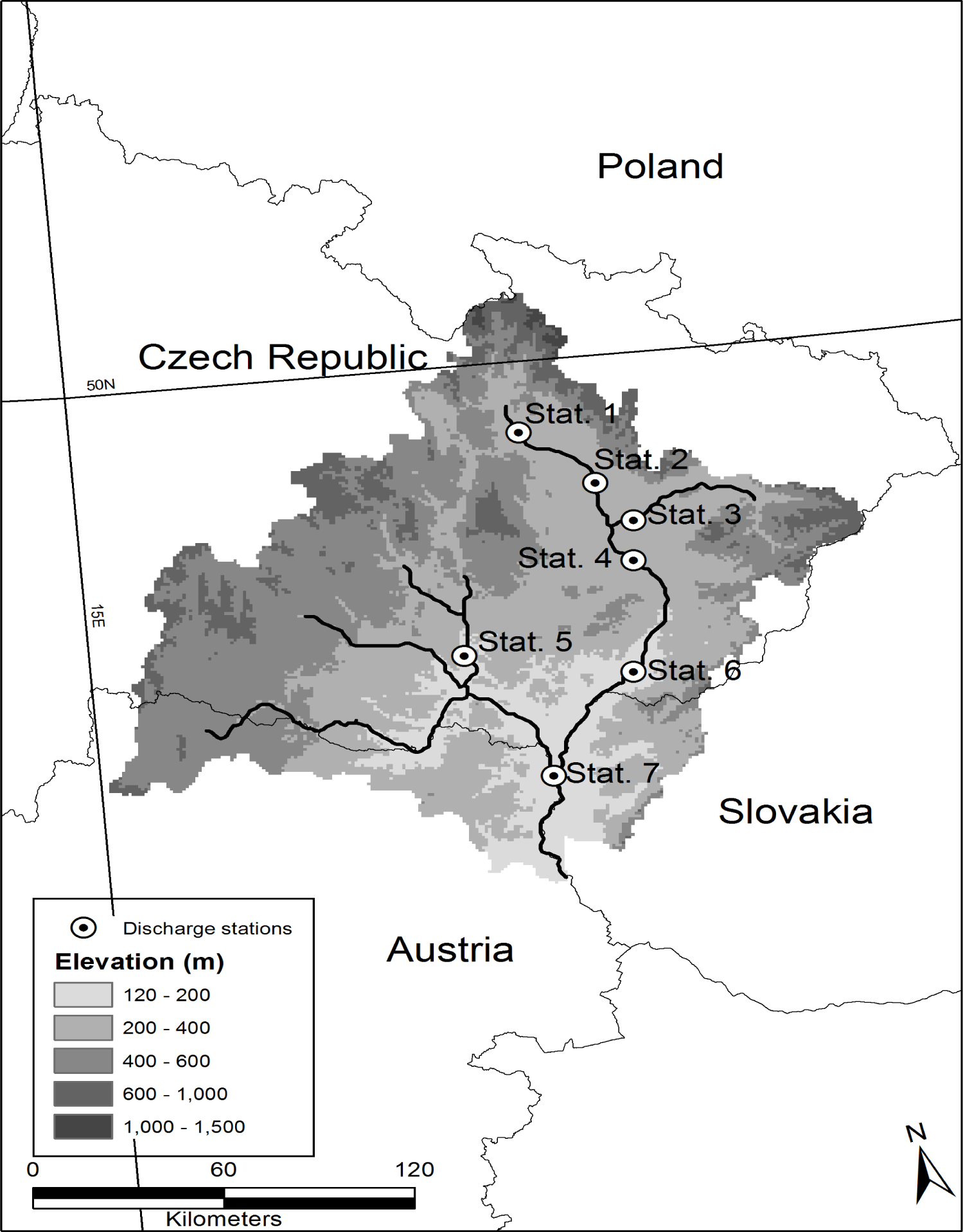
The area used for this study is the Morava River basin. The Morava River is a tributary of the Danube River, located mainly within the Czech Republic (see Figure 2). The area of the Morava River basin is around 26, 000 km2 with an elevation ranging from 120 to almost 1,500 m. Daily discharge data were available for our study area at seven gauge stations in the Morava River basin. A smaller part of this basin (8, 000 km2), upstream of the Kromericz gauging station, has also been used for preliminary experiments.
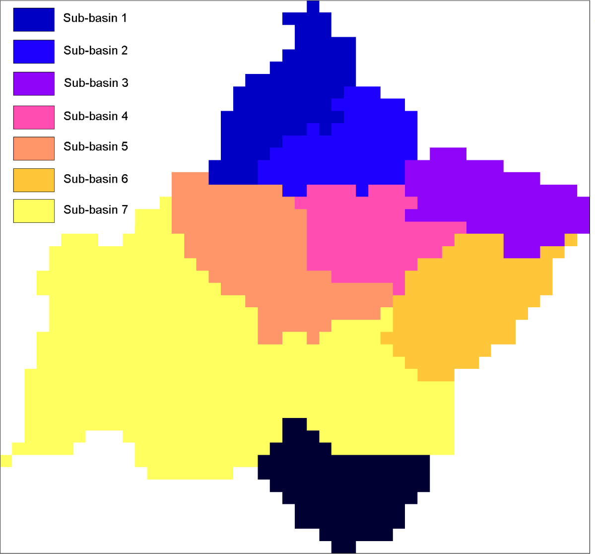
In this work, the state variable and the observation state of the particle filter have been defined in two different ways. The first approach only considers one part of the Morava basin (the study area will be described in more details in part 4.2), given by the upstream area of the Kromericz gauging station (station 4 in Figure 2). This area is represented in Figure 3 by the sub-basins 1, 2, 3 and 4 altogether. The state variable and the observation state have been defined by summing the SCA values of all pixels within this area. Consequently, the x and y vectors in Equation (1) are 1-dimensional. The basin upstream of the Kromericz gauging station has an area of 8, 000 km2 only, which allows assuming that the snow conditions are more homogeneous than in the complete Morava River basin (26, 000 km2). This size can be considered as very large, but at the scale of Europe, and for the European Flood Awareness System especially, it represents a rather small river basin. The aim of the experiments realized in this area was to consider a simple case where multi-dimensionality would not be a problem in the data assimilation algorithm. Moreover, this particular river basin is almost not influenced by human interaction.
The second approach was to consider the whole Morava basin. Given the larger area and heterogeneities, this basin has not been considered as one whole. It was decided to split this basin into seven areas (Figure 3) obtained from the drainage areas of the seven gauge stations where we had observations (called sub-basins). The state variable and the observation state are consequently vectors of dimension 7, each vector element containing the sum of the SCA values of all pixels within each sub-basin. It is important to note that the term “sub-basin” designs the area upstream of a given gauge station excluding the area upstream of another upstream station.
Experiments were carried out for the period 10 January 2004 to 10 December 2006. This period could not be extended because no discharge data were available for the stations for a longer period. We acknowledge that it would have been better not to begin and end the data assimilation process in the middle of the snow season, however in our case it would have meant reducing the dataset to only two snow seasons. In order to have realistic model states at the beginning of the data assimilation process, the model simulations started during the summer 2003 without data assimilation activated. The assimilation timestep (i.e., frequency of assimilation) was variable, from seven days—which we considered a reasonable compromise between the computing time and the time evolution of the snow cover—to a daily time-step, including 2-day and 3-day time-steps. Testing higher frequencies was not possible since the time step of the model is 1 day, and testing frequencies of more than one week seems too coarse for having a sufficiently positive impact on discharges. The assimilation was not performed during summer (i.e., from 1 May to 31 October of each year). The period of assimilation (from 1 November to 30 April of each year) usually includes the complete snow accumulation and snow melt periods for an area such as the Morava River basin.

4.3. Sources of Errors

Simulation of snow in LISFLOOD is mainly influenced by three factors: precipitation, temperature, and snow-melt coefficient. Hence, random errors have been added to these factors in order to generate the particles for the particle filter, which aim at estimating the probability density functions of these parameters. For the experiments performed on the area upstream of the Kromericz station, the parameters have been perturbed uniformly on the whole area. For the experiments realized on the whole Morava basin, the parameters have been perturbed uniformly on each sub-basin area. The precipitation fields were multiplied by a value between 0.5 and 1.5 on each zone, drawn from a uniform distribution on a daily basis. For the temperature, a value from a uniform distribution between −3 °C and +3 °C was added to each zone on a daily basis. This value is realistic; it is only slightly higher than the RMSE reported in [62], for example. Finally, the snow-melt coefficient was created with a uniform distribution for each zone in the range of the usual values of the calibrated parameter for LISFLOOD (between 2.5 and 5.5 mm ·° C−1 · day−1). During summer, there is no data assimilation performed, the perturbed meteorological fields have been replaced by the observed fields, and particles have not been resampled (in the case of the particle filter).

4.4. Definition of the Scores Used

Two different scores have been used in this study: the Ratio-RMSE (for snow) and the Nash criterion (for discharges). The scores are computed in this article for a vector z(t), that contains for each day of the period, even for the experiments running at a lower frequency than the daily one, the average of all the particles of the variable of interest (i.e., SCA or discharge) over the particles. The observation is given by o(t) and N represents the number of days of the vectors. The Ratio-RMSE is the classical RMSE divided by the average of the observation:
Ratio RMSE = 1 o ¯ 1 N t ( z ( t ) o ( t ) ) 2
The Ratio-RMSE is equal to 0 for simulations perfectly fitting the observations and is unbounded by above. The Nash criterion ([31]) is:
Nash = 1 t ( o ( t ) z ( t ) ) 2 t ( o ( t ) o ¯ ) 2
The Nash criterion is equal to 1 for discharges perfectly fitting the observations and is unbounded by below. In these equations, the average of observations ō is defined as:
o ¯ = 1 N t o ( t )
The SCA scores are computed for the whole area and for the whole study period (10 January 2004–10 December 2006), even for summer periods, for which no assimilation was performed. The discharges scores are computed for each station (only one for the “Kromericz” experiments, and seven for the whole Morava River basin) and averaged, if necessary, for the same study period.

5. Assimilation of the Area Upstream of the Kromericz Station

The results will be presented as follows: first, data assimilation on the area upstream of the Kromericz station will be discussed (Section 5). Then, the complete Morava catchment will be considered (Section 6). For each case, tests on synthetic experiments will be first processed (Section 5.1 and 6.1), and then experiments using real MODIS SCA data will be processed (Sections 5.2 and 6.2). The experiments are summed up in Table 3 and linked to every subsection. In this Section 5, only the area upstream of the Kromericz station is considered. The state variable and the observation state for the particle filter are scalar values, containing the sum of the SCA values in this area. The discharge scores are computed at the outlet of this area, i.e., at the Kromericz gauge station.

5.1. Synthetic Experiments

Synthetic experiments aimed at showing the effect on discharge of SCA assimilation only with no intervention of real MODIS SCA data. For these experiments, a normal run of LISFLOOD (called “proxy”) has been utilized for providing synthetic SCA observations and synthetic observed discharges. It means that we used observations derived from meteorological stations as input for the LISFLOOD model, and we used its SWE output, converted to SCA using the SDC, as observations for the assimilation experiments. We then compared the model performance between simulations including the particle filter and simulations not using it. The latter simulations represent the “no assimilation” experiment.
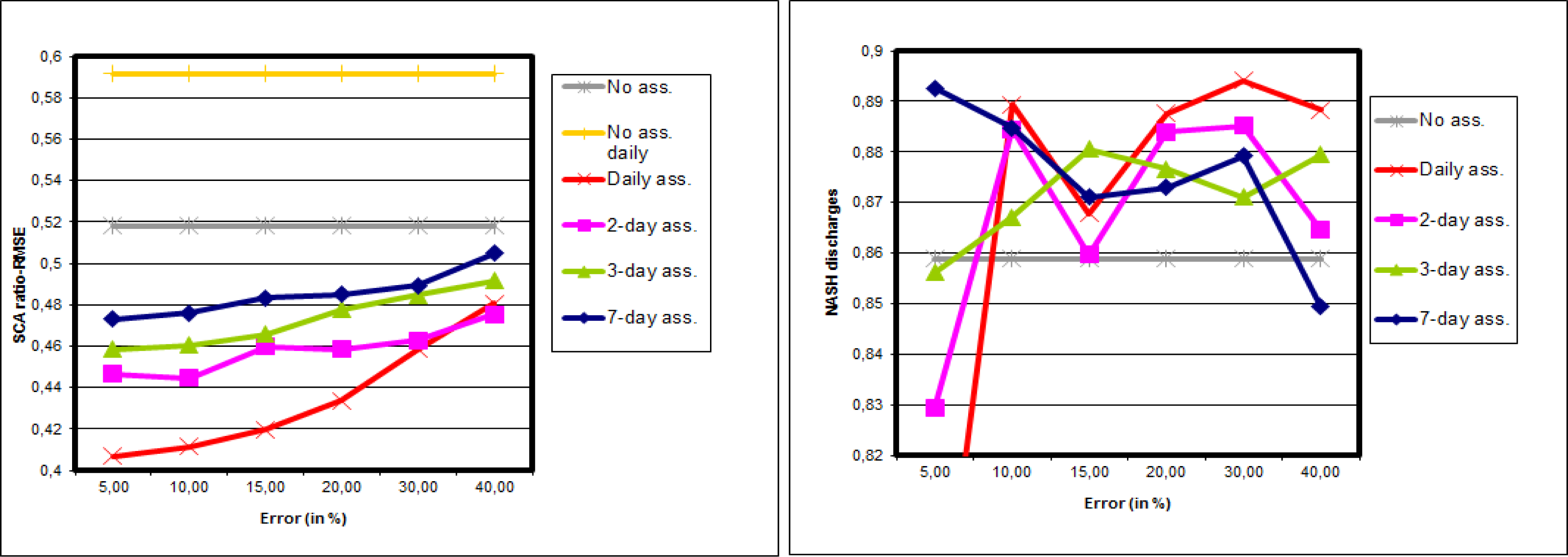
Results of the assimilation of synthetic SCA data in LISFLOOD with the particle filter are presented here for 50 particles. Figure 4 shows the impact of both the observation error and the frequency of SCA assimilation on SCA (left part) and discharge (right part) average. The reference values (i.e., without assimilation but with perturbed input) are shown as a grey line. The error intensity is irrelevant for this reference value (there is only one experiment, and no assimilation—and thus no error—is used), but it is displayed for each error intensity in order to facilitate interpretation of the graphs.
It is clear from the left part of Figure 4 that the particle filter improved the SCA, since all ratio-RMSE scores are closer to 0 than the reference one. Furthermore, it can also be observed that the lower the observation error, the larger the improvement in SCA. The frequency of assimilation also has an impact: the best results are indeed obtained for a daily assimilation, whereas a 7-day assimilation has a poorer impact. The right part of Figure 4 shows that the average discharge is also improved for every experiment, with Nash values very close to 1. The efficiency of the assimilation experiments is quite constant when the observation error or the frequency is modified. The only remarkable feature is observed for the 7-day assimilation experiment, which seems less efficient for observation error values of 30% or 40%. Since these are the experiments with the highest errors and the lowest frequencies, it is logical to observe that their impact on discharges is lower (i.e., the scores are closer to reference).
The same experiments have been performed with 200 particles (results not presented). The results for SCA and discharge showed a similar behaviour as for 50 particles. The Ratio-RMSE score for SCA was slightly improved and the Nash criterion for discharge was also slightly improved. Stronger improvements were seen for low error intensities (5%–15%). It is noticeable that the curves are smoother due to the increase of the number of particles.

5.2. Real Experiments

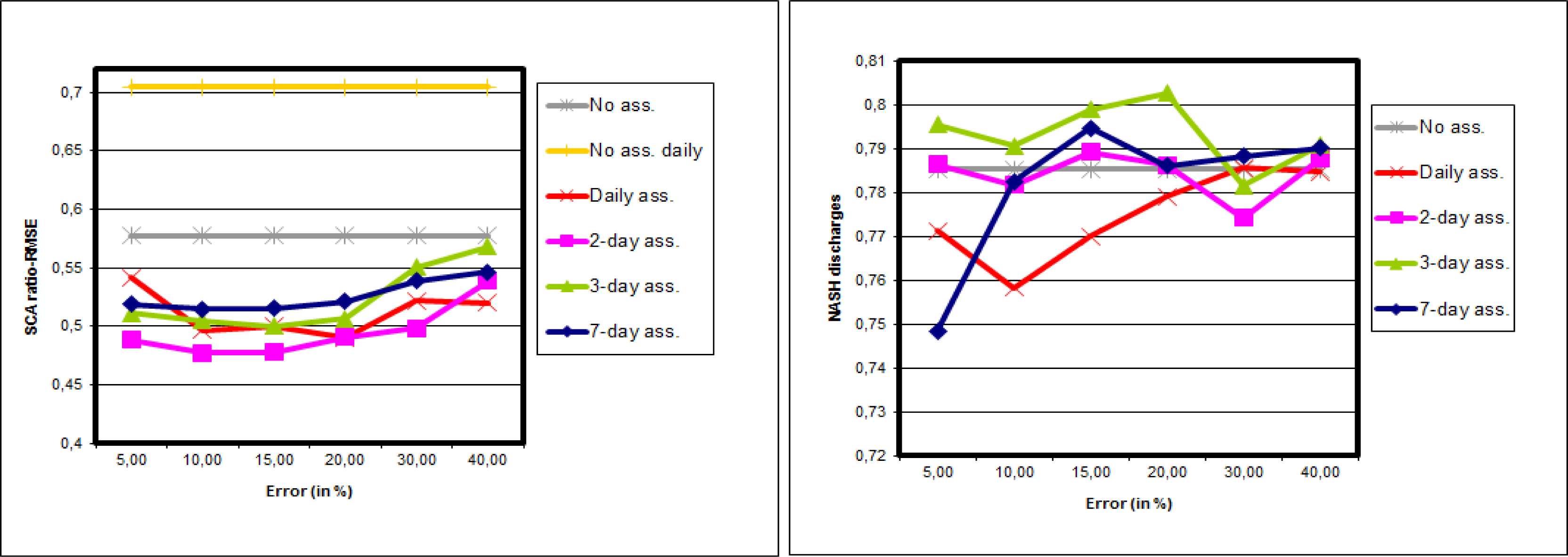
In this Section 5.2, the assimilation of real MODIS SCA data is described. Results of the assimilation of real MODIS SCA with the particle filter (50 particles) are given in Figure 5. On the left part of this figure the evolution of the SCA ratio-RMSE with observation error and assimilation frequency is given. Note that for the daily assimilation experiments, daily MODIS SCA data have been used as observations. Consequently, it has been necessary to compare the no-assimilation experiment to both the composite MODIS SCA (this is the “No ass.” curve) and the daily MODIS SCA (“No ass. daily” curve) on Figure 5. For better readability, the scores of the proxy run are not plotted in the figure: the proxy SCA has a ratio-RMSE of 0.51 compared with the composite MODIS and 0.50 compared with the daily MODIS; the proxy discharges have a Nash of 0.85.
It is clear from the left part of Figure 5 that the particle filter improves the SCA of the LISFLOOD model on the Kromericz station upstream basin. Similarly to the synthetic experiments, the smaller the observation error, and the higher the assimilation frequency, the better is the improvement. Comparison of the daily assimilation experiment curve and the No ass. daily curve shows that the improvement provided by the assimilation is substantial (from 0.06 to 0.11 Nash improvement). The impact of the particle filter (50 particles) on the Kromericz station discharge is presented in the right panel of Figure 5. Only adding perturbations to the input already brought a slight improvement to the Nash criterion of the average discharge (the “No ass. daily” curve is around 0.86 and the proxy run performed a Nash score of 0.85). From this Figure 5 we can also see that not all experiments improved the quality of the discharges. High frequency experiments with low observation error, and low frequency experiments with high observation error, deteriorated the Nash scores.
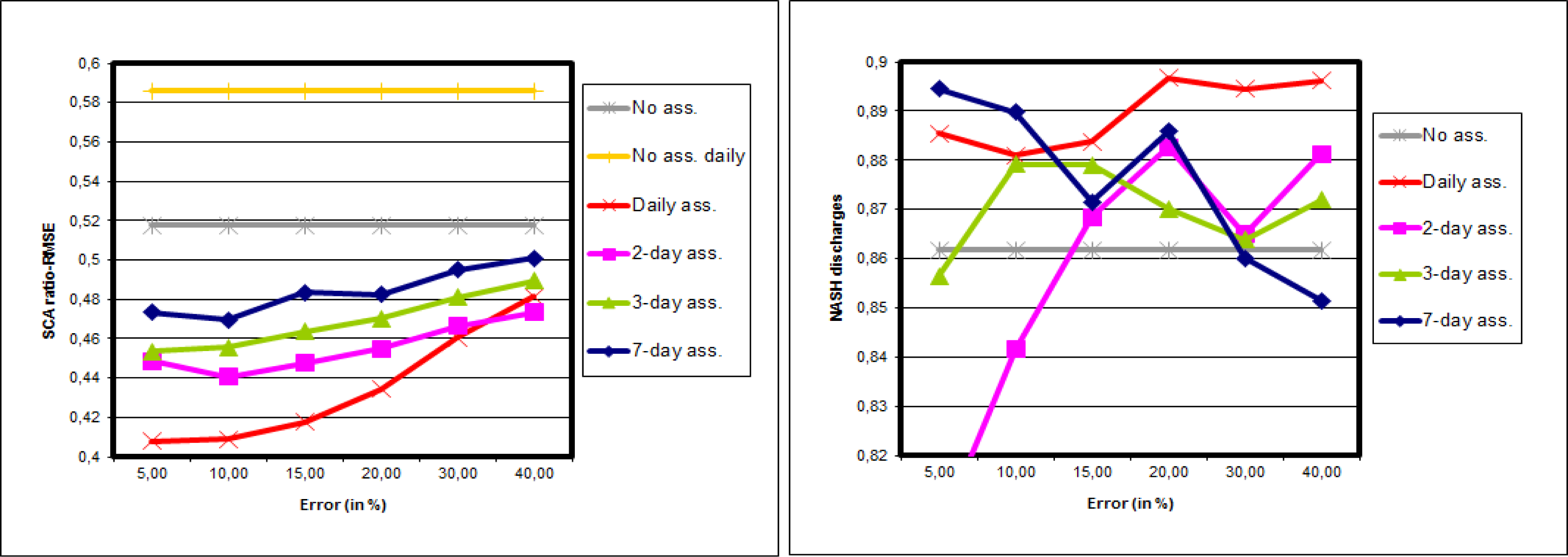
Experiments realized with 200 particles lead to the same conclusions (Figure 6). Comparing this figure with Figure 5 shows that the improvement of the LISFLOOD SCA due to the increase of the number of particles is very low. However, in the daily experiments the Nash criterion is significantly improved by the higher number of particles, whereas the other experiments do not exhibit clear modifications.

6. Assimilation on the Whole Morava Basin

In these experiments, the whole Morava basin as presented in Figure 2 is considered. The state variable and the observation state are 7-dimensional vectors, containing the sum of the SCA values on each sub-basin described in Figure 3. The discharge scores are computed on average for the seven stations and the SCA scores are computed for the whole area. Tests have been performed where the Morava basin is considered as a whole (i.e., 1-dimensional vectors) similarly to the Kromericz upper basin set of experiments (not shown here), but they were not conclusive. This was caused by the fact that spatial heterogeneities are much more important in a large-scale basin, such as the Morava (26, 000 km2), compared with the much smaller Kromericz basin (8, 000 km2). In such a case, it is very difficult to make the model SCA to correspond with MODIS SCA observations on a large area. This justifies the division of the Morava basin in seven more homogeneous zones in the following. The experiments described in this Section 6 are summed up in Table 3 and linked to every subsection.

6.1. Synthetic Experiments

Figure 7 shows the results of synthetic experiments with 50 particles on the whole Morava basin. Figure 7 left leads to similar conclusions as for the synthetic experiments for the Kromericz case. In other words: the SCA is improved for all intensities of observation error, and for all frequencies. The improvement is also higher for high frequency assimilations and for low observation errors. On Figure 7 right the impact of synthetic SCA data on discharges is shown. All experiments show a Nash increase when compared with the reference, whatever the observation error used, and whatever the frequency of assimilation.
Synthetic experiments with 200 particles show that the improvement of SCA and discharges is higher than within the experiments with only 50 particles (Figure 8).

6.2. Real Experiments

The assimilation of real MODIS SCA data on the whole Morava basin with the particle filter is presented in this Section 6.2. Results are shown in Figure 9 for 50 particles. All the experiments show a clear improvement of the LISFLOOD SCA compared with their respective no-assimilation experiments (left panel of Figure 9). This improvement seems better for intermediate values of observation error. However, an improvement is not necessarily observed when compared with the proxy, which has a ratio-RMSE equal to 0.52 when evaluated against composite MODIS and to 0.55 when evaluated against daily MODIS. In fact, the no-assimilation experiments have SCA ratio-RMSE scores that are worse than the proxy score, and for some experiments this deterioration of scores is only partially recovered by the particle filter experiments. This is especially the case for the 7-day assimilation experiments which have SCA ratio-RMSE scores higher (i.e., worse) than the proxy. Improvements are observable (even if low) for all the other experiments except for observation error of 30% and 40%, which shows that under certain conditions the particle filter is efficient for improving SCA from real MODIS SCA.
The effect of the particle filter on discharge is different (Figure 9 right).This figure shows that the discharge is improved by the perturbations, since the no-assimilation experiment has a Nash 0.02 point higher than the 0.76 Nash of the proxy. However, discharge is adversely affected by the particle filter for the case of the daily assimilation. When not deteriorated by data assimilation (with 2-, 3-, and 7-day frequencies), only low improvements of discharge can be observed (0.02 at maximum) in this figure in comparison with the no-assimilation experiment. The results of experiments with 200 particles (not shown here) lead to similar results.

7. Discussions

Every experiment showed that the improvement of SCA is dependent on the frequency of assimilation and on the observation error used. It is quite straightforward that the higher the frequency, the better the efficiency of assimilation will be, because when the SCA is not improved between each assimilation timestep, it allows the input and model errors to affect adversely the SCA quality without hindrance. Also the lower the observation error, the more the assimilation will trust the observations (i.e., the synthetic SCA or the MODIS SCA) and so the better the LISFLOOD SCA will be.
A simple 1-dimensional experiment on the area upstream of the Kromericz station showed that the quality of both average SCA and average discharges are clearly improved when synthetic SCA data are assimilated using the particle filter. This indicates the theoretical potential of the particle filtering for improving discharges via satellite SCA assimilation. Regarding the dimension of the problem, experiments on the complete Morava basin (7-dimensional experiment) showed improvements for both SCA and discharges for the synthetic case. This proves that the use of the particle filter is a suitable method for improving discharges and can deal with heterogeneity of snow within the complete basin. The particle filter respects the mass balance by adjusting the entire trajectory of the LISFLOOD SCA to fit the MODIS SCA. There is no trajectory break (as it would be for the Ensemble Kalman filter for example) that would provoke the non-conservation of the mass balance. In other words, to decrease SCA, the particle filter needs to melt the snow within the model, not to remove it from the system, so this snow amount will naturally increase the river discharge. This result shows that extending the kind of assimilation we tested in this work to larger areas (for example entire Europe) will require either a high number of particles, which will be limited by the computer power available, or an optimisation of the implementation of the particle filter (for example in the way the area is cut). It seems difficult to find the best intensity of observation error or the best frequency of assimilation for the synthetic experiments, the trends were not clear for discharges. This maybe due to the fact that the scores were already quite good (Nash close to 1) and thus the experiments are not able to have clear differences of performance.
Applying the particle filter on the area upstream of the Kromericz station for a real case experiment (i.e., assimilation of MODIS SCA) also lead to an improvement of SCA (always) and discharges (in most of the cases). When the observation error used is either very low or very significant, discharges could be deteriorated. These extreme cases (under- and over-confident with the observations) clearly show that a balance has to be found in the setup of the assimilation experiments, as is the case for every assimilation algorithm. Intermediate experiments show an improvement of the Nash criterion of more than 0.01 in all cases but two. The improvement of discharge remains weak, but considering that the Nash criterion was already high (0.86) and that this improvement is observed for an important number of tests, this shows that the real MODIS SCA data do increase the quality of discharges when they are assimilated by the particle filter.
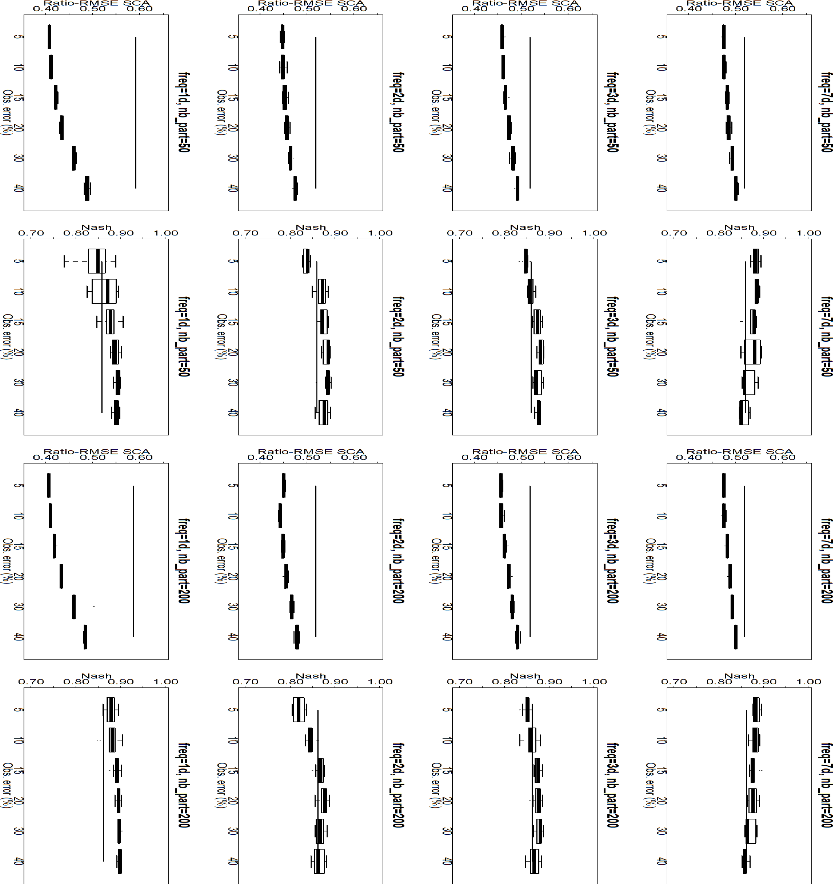
Regarding the chaotic shapes of Nash curves with observation error variations (right part of Figures 5 and 9), it is first important to note that this chaotic aspect is not observed for the SCA curves. The strong variation in the Nash curves suggests that the particle filter always selects the best samples of SCA values. With a slightly different selection of SCA values, it is clear that the Ratio-RMSE scores will not be very different. However, these SCA values result in SWE values that can differ significantly from each other (because the same SCA value, when it is equal to 1, can cover an important range of SWE values for each pixel). These differences on SWE have an impact on discharges which is likely the reason for the erratic behaviour of the Nash scores. In order to verify that the conclusions we drew in this paper on single experiments (in the sense that for each frequency of assimilation, and for each observation error, we performed only one experiment for a given basin) are correct, we reproduced each experiment nine times. In total we obtained a set of ten (9 + 1) experiments, for each frequency of assimilation, and for each observation error. These experiments are summarized for the area upstream of the Kromericz station with boxplots on Figure 10, for both the Ratio-RMSE on SCA and the Nash criteria. Each panel representing the Ratio-RMSE on SCA shows a clear increase if the observation error increases. The panels representing the Nash show a higher dispersion of results. This dispersion is higher for frequent assimilation with low observation error and for less frequent assimilation with high observation error. A higher number of particles seems to lower the dispersion of Nash, especially for daily assimilation, because of a better representation of the SCA distribution.
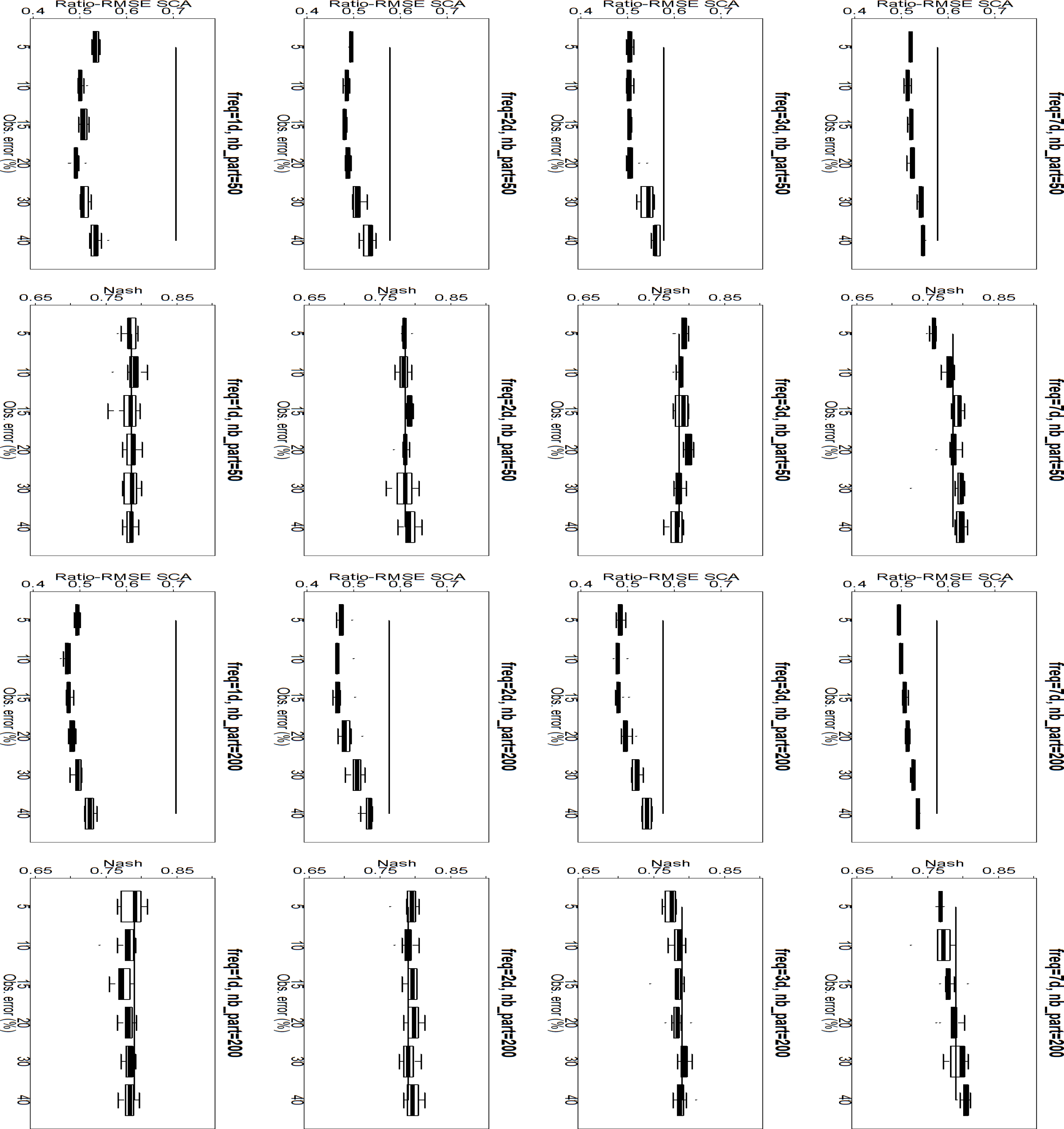
MODIS SCA assimilation on the Morava basin showed lower performance of LISFLOOD on SCA and discharge than on the area upstream of the Kromericz station. This may be due to the difficulty of the particle filter to deal with our 7-dimensional problem. This difficulty has already been pointed out by some authors, including [36]. Daily assimilation of daily MODIS SCA data on the Morava basin led to an important deterioration of discharges, that is not observed for assimilation of composite MODIS SCA at any frequency or for synthetic experiments. This shows that trusting partial SCA data (since the daily data contains around 48% of missing values due to clouds) at a high frequency can adversely affect the discharges. Assimilating the composite MODIS SCA on the Morava basin does not improve significantly the discharges except for the 3-day frequency experiments, which show a small improvement of the Nash criterion except for high values of observation error. As for the Kromericz case, additional experiments were realized and are represented on Figure 11. This figure shows that the dispersion of the results is higher than for the Kromericz case, even for SCA (even though it remains limited). This figure also confirms that the improvement of Nash is never important and is highly dependent on the frequency of assimilation and on the observation error. However, we can see that the improvement sometimes observed with single experiments was representative of the behavior of the assimilation system. To summarize, the particle filter can bring improvement on discharge even on a 7-dimensional problem, but this improvement shows to be weak and sometimes not reproduced. Other studies, using the EnKF instead of the particle filter, made similar conclusions: despite of an improvement of the snow representation, the improvement of discharge is not necessarily observed ([5,19]).
To end up with the discussion, we would like to emphasize that the particle filter reduces the uncertainty in snow cover induced by the perturbations. This effect is stronger for the experiments with the most frequent assimilation. Reducing the uncertainty can provoke a so-called collapse of the particle filter, when only particles very close to the observations are kept. This is more often the case when only few particles are used. Losing the uncertainty at one assimilation time-step can make it difficult to cover a realistic range of possible states for the following assimilation timestep, and thus deteriorates scores. By increasing the number of particles to 200, a better representation of the uncertainty of snow cover is kept.

8. Conclusions

The use of snow satellite observations such as the MODIS (Moderate Resolution Imaging Spectroradiometer) SCA (Snow Cover Area) data has received increased attention in recent studies. We presented here the benefits of using the particle filter for assimilating the MODIS SCA in the distributed hydrological LISFLOOD model. The assimilation was applied to all or part of the Czech Morava River basin, a tributary of the Danube, for a time-period of three years. The uncertainty in precipitation, temperature, and the snow-melt coefficient parameter was taken into account by using random distributions. The impact of the intensities of observation error, as well as the frequency of assimilation, have been assessed. Furthermore, the importance of the number of members or particles has been investigated.
In order to validate the assimilation algorithms, synthetic experiments have been performed. They showed the positive impact of the particle filter for SCA and discharges before real MODIS SCA assimilation. Moreover, this study showed that the particle filter is a suitable tool for real satellite SCA assimilation in a hydrological model. By suitable, we mean that improving SCA simulation within the LISFLOOD model with SCA assimilation should improve discharge simulation of the LISFLOOD model. Application to real cases of the MODIS SCA assimilation with the particle filter seems promising, especially for relatively small areas. In a small basin (8, 000 km2), assimilation results were positive for discharges improvement. However, dealing with spatial heterogeneities seems more difficult, which makes the algorithm poorly efficient (even if one could consider that as already being interesting) or even counter-productive when applied on a larger area (the entire Morava River, 26, 000 km2).
Despite of these poor results on the complete Morava basin, the positive results on the area upstream of the Kromericz station indicate that there is room for obtaining an efficient system on larger (i.e., multi-dimensional) basins. Improving the way uncertainty is represented could for example lead to better results. Moreover, giving the same importance to each sub-basin when calculating the particle weight may be improved by a better distribution (more importance to more snowy areas). Finally, the use of reliable satellite SWE (Snow Water Equivalent) or snow-depth data is also a possible way to improve the representation of snow in LISFLOOD and will probably be investigated in the future. The limitation to these data is of course that satellite SWE is still of poor quality, and that snow-depth data is not representative of the snow cover for large areas.

Acknowledgments

The authors would like to thank Jalal Younis (Czech Hydro-meteorological Institute) for providing the discharge observations in the Morava basin. Four anonymous reviewers provided useful suggestions.

Conflicts of Interest

The authors declare no conflict of interest.

References

  1. Nelson, K.; Kurc, S.A.; John, G.; Minor, R.; Barron-Gafford, G.A. Influence of snow cover duration on soil evaporation and respiration efflux in mixed-conifer ecosystems. Ecohydrology 2013. [Google Scholar] [CrossRef]
  2. Barnett, T.P.; Dumenil, L.; Schlese, U.; Roechner, E.; Latif, M. The effects of Eurasian snow cover on regional and global climate variations. J. Atmos. Sci 1989, 46, 66–685. [Google Scholar]
  3. Boone, A.; Etchevers, P. An intercomparison of three snow schemes of varying complexity coupled to the same land-surface model: Local scale evaluation at an Alpine site. J. Hydrometeorol 2001, 2, 374–394. [Google Scholar]
  4. Decker, K.L.M.; Wang, D.; Waite, C.; Scherbatskoy, T. Snow removal and ambient air temperature effects on forest soil temperatures in northern Vermont. Soil Sci. Soc. Am. J 2003, 67, 1234–1242. [Google Scholar]
  5. Clark, M.P.; Slater, A.G.; Barrett, A.P.; Hay, L.E.; McCabe, G.J.; Rajagopalan, B.; Leavesley, G.H. Assimilation of snow covered area information into hydrologic and land-surface models. Adv. Water Resour 2006, 29, 1209–1221. [Google Scholar]
  6. Zaitchik, B.; Rodell, M. Forward-looking assimilation of MODIS-derived snow-covered area into a land surface model. J. Hydrometeorol 2009, 10, 130–148. [Google Scholar]
  7. Aksoy, A.; Aberson, S.D.; Vukicevic, T.; Sellwood, K.J.; Lorsolo, S.; Zhang, X. Assimilation of high-resolution tropical cyclone observations with an ensemble kalman filter using NOAA/AOML/HRD’s HEDAS: Evaluation of the 2008–11 vortex-scale analyses. Mon. Wea. Rev 2013, 141, 1842–1865. [Google Scholar]
  8. Pu, Z.; Zhang, H.; Anderson, J. Ensemble Kalman filter assimilation of near-surface observations over complex terrain: Comparison with 3DVAR for short-range forecasts. Dyn. Meteorol. Oceanogr. 2013, 65. art. no. 19620.. [Google Scholar]
  9. Sun, C.; Hao, Z.; Ghil, M.; Neelin, J.D. Data assimilation for a coupled ocean-atmosphere model. Part I: Sequential state estimation. Mon. Wea. Rev 2002, 130, 1073–1099. [Google Scholar]
  10. Reichle, R.H.; McLaughlin, D.B.; Entekhabi, D. Hydrologic data assimilation with the Ensemble Kalman Filter. Mon. Wea. Rev 2002, 130, 103–114. [Google Scholar]
  11. Crow, W.T.; Ryu, D. A new data assimilation approach for improving runoff prediction using remotely-sensed soil moisture retrievals. Hydrol. Earth Syst. Sci 2009, 13, 1–16. [Google Scholar]
  12. Salamon, P.; Feyen, L. Assessing parameter, precipitation, and predictive uncertainty in a distributed hydrological model using sequential data assimilation with the particle filter. J. Hydrol 2009, 376, 428–442. [Google Scholar]
  13. Thirel, G.; Martin, E.; Mahfouf, J.-F.; Massart, S.; Ricci, S.; Habets, F. A past discharges assimilation system for ensemble streamflow forecasts over France—Part 1: Description and validation of the assimilation system. Hydrol. Earth Syst. Sci 2010, 14, 1623–1637. [Google Scholar]
  14. Liu, Y.; Weerts, A.H.; Clark, M.; Franssen, H.-J.H.; Kumar, S.; Moradkhani, H.; Seo, D.-J.; Schwanenberg, D.; Smith, P.; van Dijk, A.I.J.M.; et al. Advancing data assimilation in operational hydrologic forecasting: progresses, challenges, and emerging opportunities. Hydrol. Earth Syst. Sci 2012, 16, 3863–3887. [Google Scholar]
  15. Rodell, M.; Houser, P.R. Updating a land surface model with MODIS-derived snow cover. J. Hydrometeorol 2004, 8, 1064–1075. [Google Scholar]
  16. Andreadis, K.M.; Lettenmaier, D.P. Assimilating remotely sensed snow observations into a macroscale hydrology model. Adv. Water Resour 2006, 29, 872–886. [Google Scholar]
  17. Su, H.; Yang, Z.-L.; Niu, G.-Y.; Dickinson, R.E. Enhancing the estimation of continental-scale snow water equivalent by assimilating MODIS snow cover with the ensemble Kalman filter. J. Geophys. Res. 2008, 113. [Google Scholar] [CrossRef]
  18. Bavera, D.; de Michele, C. Snow water equivalent estimation in the Mallero basin using snow gauge data and MODIS images and fieldwork validation. Hydrol. Process 2009, 23, 1961–1972. [Google Scholar]
  19. Roy, A.; Royer, A.; Turcotte, R. Improvement of springtime streamflow simulations in a boreal environment by incorporating snow-covered area derived from remote sensing data. J. Hydrol 2010, 390, 35–44. [Google Scholar]
  20. Yatheendradas, S.; Peters-Lidard, C.D.; Koren, V.; Cosgrove, B.A.; De Goncalves, L.G.G.; Smith, M.; Geiger, J.; Cui, Z.; Borak, J.; Kumar, S.; et al. Distributed assimilation of satellite-based snow extent for improving simulated streamflow in mountainous, dense forests: An example over the DMIP2 western basins. Water Resour. Res. 2012, 48. [Google Scholar] [CrossRef]
  21. Liu, Y.; Peters-Lidard, C.D.; Kumar, S.; Foster, J.L.; Shaw, M.; Tian, Y.; Fall, G.M. Assimilating satellite-based snow depth and snow cover products for improving snow predictions in Alaska. Adv. Water Resour 2013, 54, 208–227. [Google Scholar]
  22. Pulliainen, J.; Hallikainen, M. Retrieval of regional snow water equivalent from space-borne passive microwave observations. Remote Sens. Environ 2001, 75, 76–85. [Google Scholar]
  23. Dong, J.; Walker, J.P.; Houser, P.R. Factors affecting remotely sensed snow water equivalent uncertainty. Remote Sens. Environ 2005, 97, 68–82. [Google Scholar]
  24. Parajka, J.; Blöschl, G. Validation of MODIS snow cover images over Austria. Hydrol. Earth Syst. Sci 2006, 10, 679–689. [Google Scholar]
  25. Gafurov, A.; Bàrdossy, A. Cloud removal methodology from MODIS snow cover product. Hydrol. Earth Syst. Sci 2009, 13, 1361–1373. [Google Scholar]
  26. Gao, Y.; Xie, H.; Lu, N.; Yao, T.; Liang, T. Toward advanced daily cloud-free snow cover and snow water equivalent products from Terra-Aqua MODIS and Aqua AMSR-E measurements. J. Hydrol 2010, 385, 23–35. [Google Scholar]
  27. Parajka, J.; Blöschl, G. Spatio-temporal combination of MODIS images—Potential for snow cover mapping. Water Resour. Res. 2008, 44. [Google Scholar] [CrossRef]
  28. Parajka, J.; Pepe, M.; Rampini, A.; Rossi, S.; Blöschl, G. A regional snow-line method for estimating snow cover from MODIS during cloud cover. J. Hydrol 2009, 381, 203–212. [Google Scholar]
  29. Slater, A.G.; Clark, M.P. Snow data assimilation via an Ensemble Kalman Filter. J. Hydrometeorol 2006, 7, 478–493. [Google Scholar]
  30. Clark, M.P.; Vrugt, J.A. Unraveling uncertainties in hydrologic model calibration: Addressing the problem of compensatory parameters. Geophys. Res. Lett. 2006, 33. [Google Scholar] [CrossRef]
  31. Nash, J.E.; Sutcliffe, J.V. River flow forecasting through conceptual models part I—A discussion of principles. J. Hydrol 1970, 10, 282–290. [Google Scholar]
  32. Lindström, G.; Johansson, B.; Persson, M.; Gardelin, M.; Bergström, S. Development and test of the distributed HBV-96 hydrological model. J. Hydrol 1997, 201, 272–288. [Google Scholar]
  33. Thielen, J.; Bartholmes, J.; Ramos, M.-H.; de Roo, A. The European Flood Alert System—Part 1: Concept and development. Hydrol. Earth Syst. Sci 2009, 13, 125–140. [Google Scholar]
  34. Doucet, A.; de Freitas, N.; Gordon, N. Sequential Monte Carlo Methods in Practice; Springer: New York, NY, USA, 2001. [Google Scholar]
  35. Simon, D. Optimal State Estimation: Kalman, H Infinity, and Nonlinear Approaches; Wiley-Interscience: Hoboken, NJ, USA, 2006. [Google Scholar]
  36. Van Leeuwen, P.J. Particle filtering in geophysical systems. Mon. Wea. Rev 2009, 137, 4089–4114. [Google Scholar]
  37. Arulampalam, M.S.; Markell, S.; Gordon, N.; Clapp, T. A tutorial on particle filters for online nonlinear/non-Gaussian Bayesian tracking. IEEE Trans. Signal Process 2002, 50, 174–188. [Google Scholar]
  38. Chin, T.M.; Turmon, M.J.; Jewell, J.B.; Ghil, M. An ensemble-based smoother with retrospectively updated weights for highly nonlinear systems. Mon. Wea. Rev 2007, 135, 186–202. [Google Scholar]
  39. Baker, J.E. Reducing Bias and Inefficiency in the Selection Algorithm. Proceedings of the Second International Conference on Genetic Algorithms and their Application; Lawrence Erlbaum Associates: Hillsdale, NJ, USA, 1987; pp. 14–21. [Google Scholar]
  40. Moradkhani, H.; Hsu, K.-L.; Gupta, H.; Sorooshian, S. Uncertainty assessment of hydrologic model states and parameters. Water Resour. Res. 2005, 41. [Google Scholar] [CrossRef]
  41. Hall, D.K.; Riggs, G.A.; Salomonson, V.V. MODIS/Aqua Snow Cover Daily L3 Global 500m Grid V005; July 2003 to December 2006; National Snow and Ice Data Center: Boulder, CO, USA, 2006. [Google Scholar]
  42. Hall, D.K.; Riggs, G.A.; Salomonson, V.V. MODIS/Terra Snow Cover Daily L3 Global 500m Grid V005; July 2003 to December 2006; National Snow and Ice Data Center: Boulder, CO, USA, 2006. [Google Scholar]
  43. Sirguey, P.; Mathieu, R.; Arnaud, Y. Subpixel monitoring of the seasonal snow cover with MODIS at 250 m spatial resolution in the Southern Alps of New Zealand: Methodology and accuracy assessment. Remote Sens. Environ 2009, 113, 160–181. [Google Scholar]
  44. Painter, T.H.; Rittger, K.; McKenzie, C.; Slaughter, P.; Davis, R.E.; Dozier, J. Retrieval of subpixel snow-covered area, grain size, and albedo from MODIS. Remote Sens. Environ 2009, 113, 868–879. [Google Scholar]
  45. Niu, G.-Y.; Yang, Z.-L. An observation-based formulation of snow cover fraction and its evaluation over large North American river basins. J. Geophys. Res. 2007, 112. [Google Scholar] [CrossRef]
  46. Koren, V.; Schaake, J.; Mitchell, K.; Duan, Q.Y.; Chen, F.; Baker, J.M. A parameterization of snowpack and frozen ground intended for NCEP weather and climate models. J. Geophys. Res 1999, 104, 19569–19585. [Google Scholar]
  47. De Roo, A. LISFLOOD: A Rainfall-runoff Model for Large River Basins to Assess the Influence of Land Use Changes on Flood Risk. In Ribamod: river basin modelling, management and flood mitigation; Balabanis, P., Ed.; European Commission: Wallingford, UK, 1999; pp. 349–357. [Google Scholar]
  48. Van der Knijff, J.; Younis, J.; de Roo, A. LISFLOOD—A GIS-based distributed model for river basin scale water balance and flood simulation. Int. J. Geogr. Inf. Sci 2010, 24, 189–212. [Google Scholar]
  49. Karssenberg, D. The value of environmental modelling languages for building distributed hydrological models. Hydrol. Process 2002, 16, 2751–2766. [Google Scholar]
  50. Wösten, J.H.M.; Lilly, A.; Nemes, A.; Le Bas, C. Development and use of a database of hydraulic properties of European soils. Geoderma 1999, 90, 169–185. [Google Scholar]
  51. European Environment Agency. The European Topic Centre on Terrestrial Environment: Corine Land Cover raster database 2000–100m; European Environment Agency: Copenhagen, Denmark, 2000. [Google Scholar]
  52. King, D.; Daroussin, J.; Tavernier, R. Development of a soil geographical database from the soil map of the European communities. Catena 2004, 21, 37–56. [Google Scholar]
  53. Rijks, D.; Teres, J.M.; Vossen, P. Agrometeorological Applications for Regional Crop Monitoring and Production Assessment; Tech. Rep. EUR 17735 EN; Eur. Comm. Joint Res. Cent.: Ispra, Italy, 1998. [Google Scholar]
  54. Zhao, R.J.; Liu, X.R. The Xinanjiang Model. In Computer Models of Watershed Hydrology; Singh, V.P., Ed.; Water Resources Publications: Colorado, CO, USA, 1995; pp. 215–232. [Google Scholar]
  55. Todini, E. The ARNO rainfall-runoff. J. Hydrol 1996, 175, 339–382. [Google Scholar]
  56. Chow, V.T.; Maidment, D.R.; Mays, L.M. Applied Hydrology; McGraw-Hill: Singapore, 1988; p. 572. [Google Scholar]
  57. Viviroli, D.; Zappa, M.; Gurtz, J.; Weingartner, R. An introduction to the hydrological modelling system PREVAH and its pre- and post-processing tools. Environ. Model. Softw 2009, 24, 1209–1222. [Google Scholar]
  58. Finger, D.; Pellicciotti, F.; Konz, M.; Rimkus, S.; Burlando, P. The value of glacier mass balance, satellite snow cover images, and hourly discharge for improving the performance of a physically based distributed hydrological model. Water Resour. Res. 2011, 47. [Google Scholar] [CrossRef]
  59. Speers, D.D.; Versteeg, J.D. Runoff Forecasting for Reservoir Operations—The Past and the Future. In Proceedings of the 52nd Western Snow Conference; Western Snow Conference: Fort Collins, CO, USA, 1982; pp. 149–156. [Google Scholar]
  60. Anderson, E. Snow Accumulation and Ablation Model—SNOW-17; Technical Report; NWSRFS: Silver Spring, MD, USA, 2006; p. 61. [Google Scholar]
  61. Burek, P.; de Roo, A. LISFLOOD—Distributed Water Balance and Flood Simulation Model; User Manual Version December 2010; European Commission: Ispra, Italy, 2011. [Google Scholar]
  62. Quintana Seguí, P.; Le Moigne, P.; Durand, Y.; Martin, E.; Habets, F.; Baillon, M.; Canellas, C.; Franchisteguy, L.; Morel, S. Analysis of near surface atmospheric variables: Validation of the SAFRAN analysis over France. J. Appl. Meteorol. Climatol 2008, 47, 92–107. [Google Scholar]
Figure 1. The differents steps for merging MODIS maps. The Snow Cover Area (i.e., SCA) is shown here, from 0 for no snow to 1 for pixels entirely covered by snow. Details are given in the text in Section 3.
Remotesensing 05 05825f1
Figure 2. Map of the Morava basin study area (the Kromericz gauge station is the station 4).
Remotesensing 05 05825f2
Figure 3. Map of the 7 different zones used for the assimilation experiments on the Morava basin (the black part was not taken into account for the particle filter). The data assimilation experiments on the area upstream of the Kromericz station only include the zones 1, 2, 3 and 4.
Remotesensing 05 05825f3
Figure 4. SCA ratio-RMSE (left) and Nash (right) for the synthetic SCA particle filter assimilation experiments on the area upstream of the Kromericz station with 50 particles. Impact of the magnitude of the R matrix and of the frequency of assimilation is shown.
Remotesensing 05 05825f4
Figure 5. SCA ratio-RMSE (left) and Nash (right) for the real MODIS SCA particle filter experiments on the area upstream of the Kromericz station with 50 particles. The SCA proxy (not plotted) has a ratio-RMSE of 0.51 compared with the composite MODIS and 0.50 compared with the daily MODIS; the proxy discharges have a Nash of 0.85.
Remotesensing 05 05825f5
Figure 6. SCA ratio-RMSE (left) and Nash (right) for the real MODIS SCA particle filter experiments on the area upstream of the Kromericz station with 200 particles. The SCA proxy (not plotted) has a ratio-RMSE of 0.51 compared with the composite MODIS and 0.50 compared with the daily MODIS; the proxy discharges have a Nash of 0.85.
Remotesensing 05 05825f6
Figure 7. SCA ratio-RMSE (left) and Nash (right) for the synthetic SCA particle filter experiments on the whole Morava basin with 50 particles.
Remotesensing 05 05825f7
Figure 8. SCA ratio-RMSE (left) and Nash (right) for the synthetic SCA particle filter experiments on the whole Morava basin with 200 particles.
Remotesensing 05 05825f8
Figure 9. SCA ratio-RMSE (left) and Nash (right) for the real MODIS SCA particle filter experiments on the whole Morava basin with 50 particles. The SCA proxy (not plotted) has a ratio-RMSE of 0.52 compared with the composite MODIS and 0.55 compared with the daily MODIS; the proxy discharges have a Nash of 0.76.
Remotesensing 05 05825f9
Figure 10. SCA ratio-RMSE and Nash for the real MODIS SCA particle filter experiments on the area upstream of the Kromericz station. The frequency of assimilation (freq) and the number of particles (nb part) are indicated for every panel on the y-axis. The boxplots are drawn for 10 similar-condition experiments. The corresponding no-assimilation experiment is represented with a line.
Remotesensing 05 05825f10
Figure 11. SCA ratio-RMSE and Nash for the real MODIS SCA particle filter experiments on the whole Morava basin. The frequency of assimilation (freq) and the number of particles (nb part) are indicated for every panel on the y-axis. The boxplots are drawn for 10 similar-condition experiments. The corresponding no-assimilation experiment is represented with a line.
Remotesensing 05 05825f11
Table 1. Snow categories in the MODIS classification (left part) and as used for the preprocessing (right part).
MODIS ClassificationUsed Classification

ValueDataValueData
0Missing
1No decision
11NightMissing value“we don’t know”
50Cloud obscured
254Detector saturated
255Fill

25Snow-free land0No snow
37Lake or inland water
39Open water (ocean)

100Snow-covered lake ice1Snow
200Snow
Table 2. Percentage of cloud coverage, averaged over the period 10 January 2004–10 December 2006, for the different improvement methods.
Aqua+Terra+Day-1+Days-2/-3+Days-4/-5+Days-6/-7
48.633.216.89.04.9
Table 3. Summary of experiments.
AreaMethodObservationsObs. Error RangeFrequency
Section 5.1Upstr. KromericzSynthetic
Section 5.2Particle filterMODISFrom 5% to 40%1,2,3,7 days
Section 6.1Morava basinSynthetic
Section 6.2MODIS