1. Introduction
The Velodyne HDL-64E S2 laser scanner was originally conceived for competition in the Defense Advanced Research Project Agency’s (DARPA) “Grand Challenge” which required autonomous vehicles to navigate across desert terrain, and then later through an urban environment. In fact, for the urban Grand Challenge the HDL-64E S2 was used by five of the six teams who finished successfully, including the first and second place finishers [
1]. As a result of the Grand Challenge exposure, the Velodyne sensor has been a standard tool for developers of autonomous vehicles, robotics and automotive safety systems. Recently, however, this laser scanner has become a very popular choice for integration into kinematic mobile mapping platforms [
1,
2]. Evidence of this can be seen in its recent inclusion in the Google mobile mapping and smart car systems [
3]. In addition, Topcon has also announced a kinematic mapping platform using the Velodyne laser scanner [
4].
To date, most mapping applications of the Velodyne scanner have mainly targeted the medium accuracy (0.1 to 1.0 m 3D RMSE) GIS asset collection marketplace. The mobile mapping applications requiring the highest accuracy (i.e., <5 cm 3D RMSE) are mainly dominated by the systems centered on the Optech Lynx and Riegl VQ-250 laser scanners. The specifications of the Velodyne HDL-64E S2 do not match those of the Optech and Riegl scanners and therefore its use in high accuracy mobile scanning applications, such as railway and highway corridor surveys might be dismissed. However, to the authors’ knowledge no published kinematic accuracy analysis of the Velodyne HDL-64E S2 exists.
In previous work by the authors, presented in [
5], some initial static calibration analyses of the Velodyne scanner were presented. It was found that a rigorous calibration of the scanner and a slight modification of the factory calibration model improved the overall accuracy of the point cloud obtained from the scanner by a factor of three. Final 3D RMS error of the scanner was on the order of 1.3 cm. This low noise level indicated that the scanner perhaps had potential as the basis of a high accuracy mobile mapping platform. However, there were still several questions remaining to verify that the scanner could consistently obtain the accuracy required.
The results and analysis presented herein extend upon the initial analyses in [
5]. First, the remaining systemic errors noted in [
5] are examined and their root cause identified. Some additional possible calibration parameters are also identified and examined. Next, the calibration of two different Velodyne HDL-64E S2 scanners is examined over time to determine the temporal stability of the calibration parameters for the scanner. The paper concludes with an examination of the overall temporal accuracy achievable with the scanner, which shows a 25% improvement in accuracy over the standard Velodyne factory calibration.
2. Mathematical Model of the Velodyne Scanner
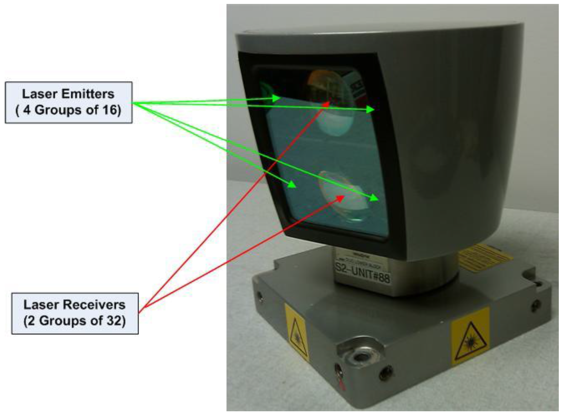
The Velodyne laser scanner consists of a rotating head which contains 64 semiconductor lasers operating at a 905 nm wavelength and firing at up to 20,000 Hz, coupled with 64 dedicated photo detectors for precise ranging. The laser-detector pairs are precisely aligned at set vertical angles to give a 26.8° vertical field of view. The sensor head rotates at speeds up to 900 rpm (15 Hz) to give a full 360° field of view and captures up to 1.3 million points per second. Detailed specifications on the HDL-64E S2 can be found in [
6]. A picture of the scanner is given in
Figure 1.
Figure 1.
The Velodyne HDL-64E S2 Scanner.
Figure 1.
The Velodyne HDL-64E S2 Scanner.
The computation of local scanner coordinates (x, y, z) for laser i of the Velodyne scanner is given by:
where:
- si
is the distance scale factor for laser i;
is the distance offset for laser i;
- δi
is the vertical rotation correction for laser i;
- βi
is the horizontal rotation correction for laser i;
is the horizontal offset from scanner frame origin for laser i;
is the vertical offset from scanner frame origin for laser i;
- Ri
is the raw distance measurement from laser i;
- ε
is the encoder angle measurement.
In the above model, the terms Ri and ε are the raw measurements provided by the scanner, whereas the other six parameters are instrument specific calibration values that are provided by Velodyne.
In examining the model for the Velodyne scanner and comparing the sensor to traditional tripod mounted instruments such as total stations it becomes apparent that additional modeling, above and beyond this formula may be required. Of particular interest is the possible non-orthogonality between the plane containing the horizontal angle encoder and the vertical axis. This would create a sinusoidal error with period of 180° for the horizontal angle measurements [
7]. In order to account for this possibility the encoder angle measurements are supplemented to include the possibility of these terms.
It should be noted that it is assumed that the 64 lasers in the Velodyne scanner are rigidly attached to the same assembly, and therefore the corrections computed by Equation (2) are common for all of the lasers. The inclusion of these errors therefore only adds an additional two unknowns to the overall model for the scanner.
3. Least Squares Adjustment Functional Model
The adjustment used for the Velodyne scanner is a plane-based calibration approach. Details of this approach for airborne scanner boresight determination or static scanner calibration are available in the literature (e.g., [
8,
9]), so a detailed development of the model is not repeated here. The observational model for the planar approach is based upon conditioning the individual LiDAR points to lie on a global planar surface. The functional model for this conditioning is given as:
where
are the unknowns of a plane l on which the LiDAR points are conditioned, and
is the vector of globally referenced LiDAR points. For a static calibration, with data collected from k locations, the j
th point can be calculated in a global coordinate frame via a rigid body transformation of the form:
where
and
are the rotational transformation matrix and translation vector between the k
th scanner space and the global coordinate frame respectively, and
is the scanner space coordinates of point j, given by Equation (1). For the static calibration procedure, the rotation and translation vectors for each of the scanner spaces k are normally unknown, and are therefore included in the adjustment as additional unknowns.
The optimal solution to the least squares adjustment for the functional model described in above can be given by the standard Gauss-Helmert adjustment model [
10]. For details on the implementation of the Gauss-Helmert adjustment model for planar constraints, the reader is referred to [
9], and to [
5] for a more detailed discussion of some of the aspects of the functional model utilized herein for the static Velodyne calibration.
4. Static Data Collection
In a period of six months at the beginning of 2010, Terrapoint had access to two Velodyne HDL‑64E S2 scanners, one which was loaned to Terrapoint for evaluation, and the second which was purchased to be integrated into a mobile scanning platform for a third party client. Access to two scanners provided Terrapoint the unique opportunity to not only verify the temporal stability of the Velodyne scanner but also to verify that the conclusions were similar for more than one scanner.
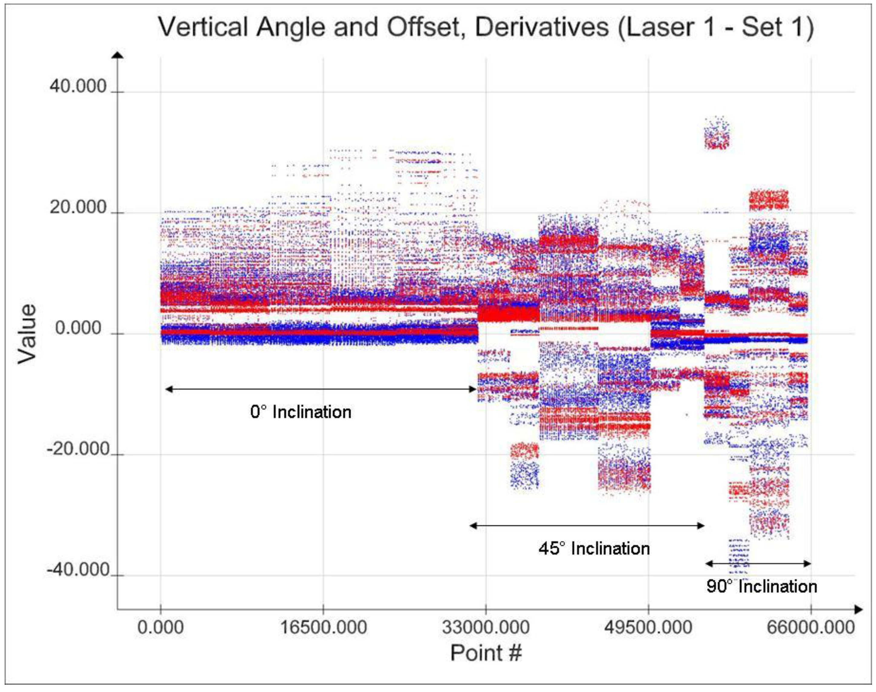
Several datasets for each scanner were collected for the purposes of static calibration and for temporal stability assessment. Herein we will focus on four datasets, two for each of the laser scanners. For consistency, these datasets will be referred to as Laser 1–Set 1, Laser 1–Set 2, Laser 2–Set 1, and Laser 2–Set 2.
All four of the datasets were collected in the same calibration area. For reference, this was also the same scene used for calibration in [
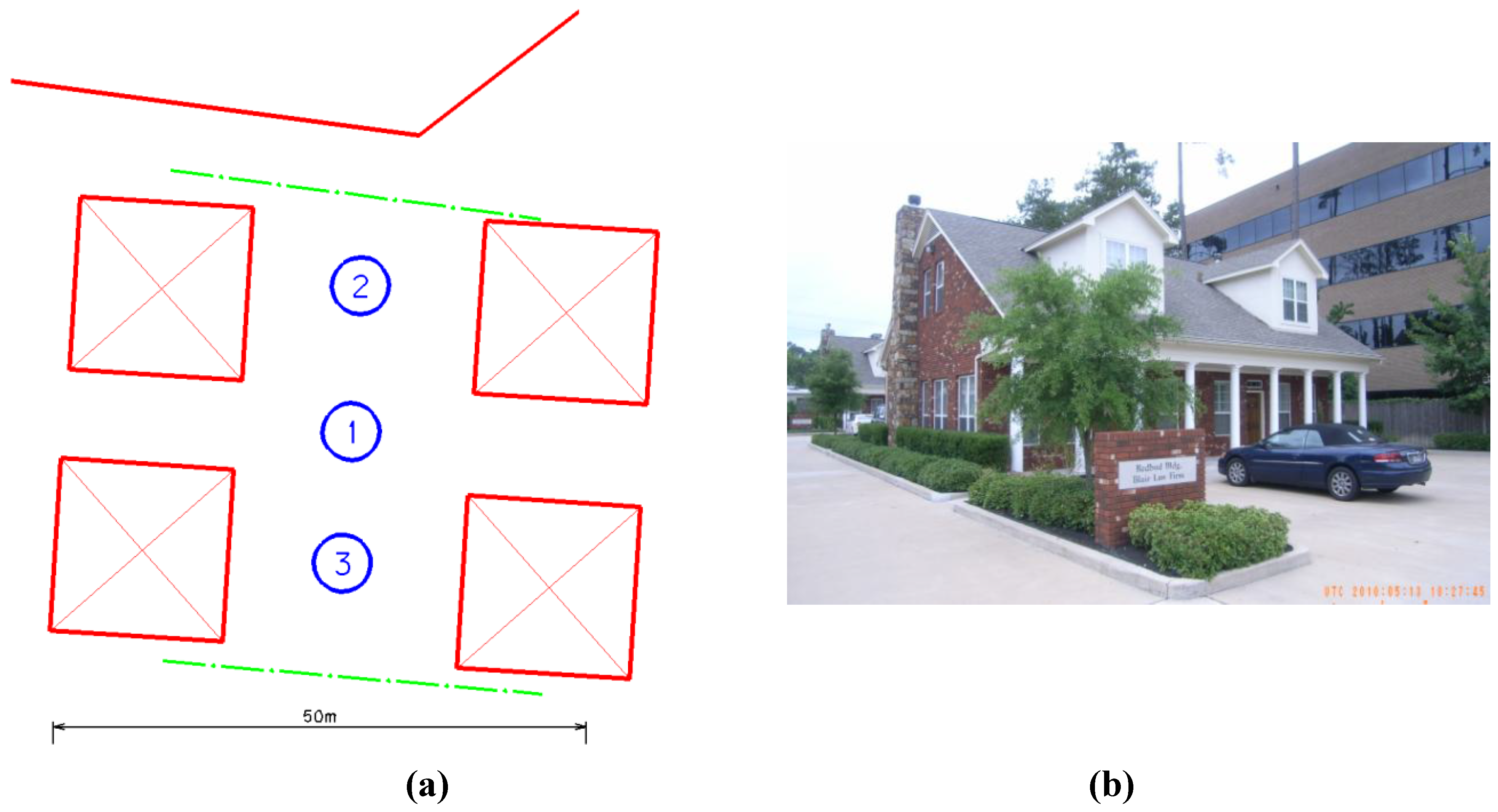
5]. Sixteen individual stations (or set-ups) of scan data were collected for each datasets. The scanner was placed at one of three scan locations, and was inclined at an angle of 0°, 45°, or 90°. The azimuth of the scanner for the each of the collections was also varied. A schematic of the scanned scene, along with a representative photo of one of the buildings is given in
Figure 2. The scan locations, inclinations and azimuth for each of the 16 set-ups are given in
Table 1. Note that the scan location numbers refer to the blue numbered circles in
Figure 2(a).
Figure 2.
Experimental Data Collection Layout. (a) Scan locations in blue, buildings in red, and fence in green, and (b) photo of the building in Northwest Quadrant (taken at Scan Location 1).
Figure 2.
Experimental Data Collection Layout. (a) Scan locations in blue, buildings in red, and fence in green, and (b) photo of the building in Northwest Quadrant (taken at Scan Location 1).
Table 1.
Position and Orientation of 16 Scans in Each of the Four Datasets.
Table 1.
Position and Orientation of 16 Scans in Each of the Four Datasets.
| Set-Up # | Scan Location | Inclination (°) | Azimuth (°) |
|---|
| 1 | 1 | 0 | 90 |
| 2 | 1 | 0 | 270 |
| 3 | 2 | 0 | 0 |
| 4 | 2 | 0 | 180 |
| 5 | 3 | 0 | 0 |
| 6 | 3 | 0 | 180 |
| 7 | 1 | 45 | 45 |
| 8 | 1 | 45 | 135 |
| 9 | 1 | 45 | 225 |
| 10 | 1 | 45 | 315 |
| 11 | 2 | 45 | 0 |
| 12 | 3 | 45 | 180 |
| 13 | 1 | 90 | 45 |
| 14 | 1 | 90 | 135 |
| 15 | 1 | 90 | 225 |
| 16 | 1 | 90 | 315 |
For each dataset, between 120 and 150 planar surfaces were extracted from all sixteen set-ups. The planar surfaces were chosen to provide an even distribution of points from each set-up, at varying planar inclination angles, and from each laser in the Velodyne sensor array. The analysis in [
5] had shown that planar points with higher incidence angles (
i.e., >70°) exhibited larger residuals, consistent with studies of other instruments (e.g., [
7]). However, even though these points showed higher residuals, their inclusion in the adjustments was not found to significantly influence the final estimated calibration parameters for the scanner. Therefore, for the analysis presented below, observations at all incidence angles were included.
6. Temporal Stability of the Scanner
To examine the temporal stability of the scanners, two separate calibration datasets were collected with each scanner, separated by a short period of time and a complete cool-down and restart of the lasers.
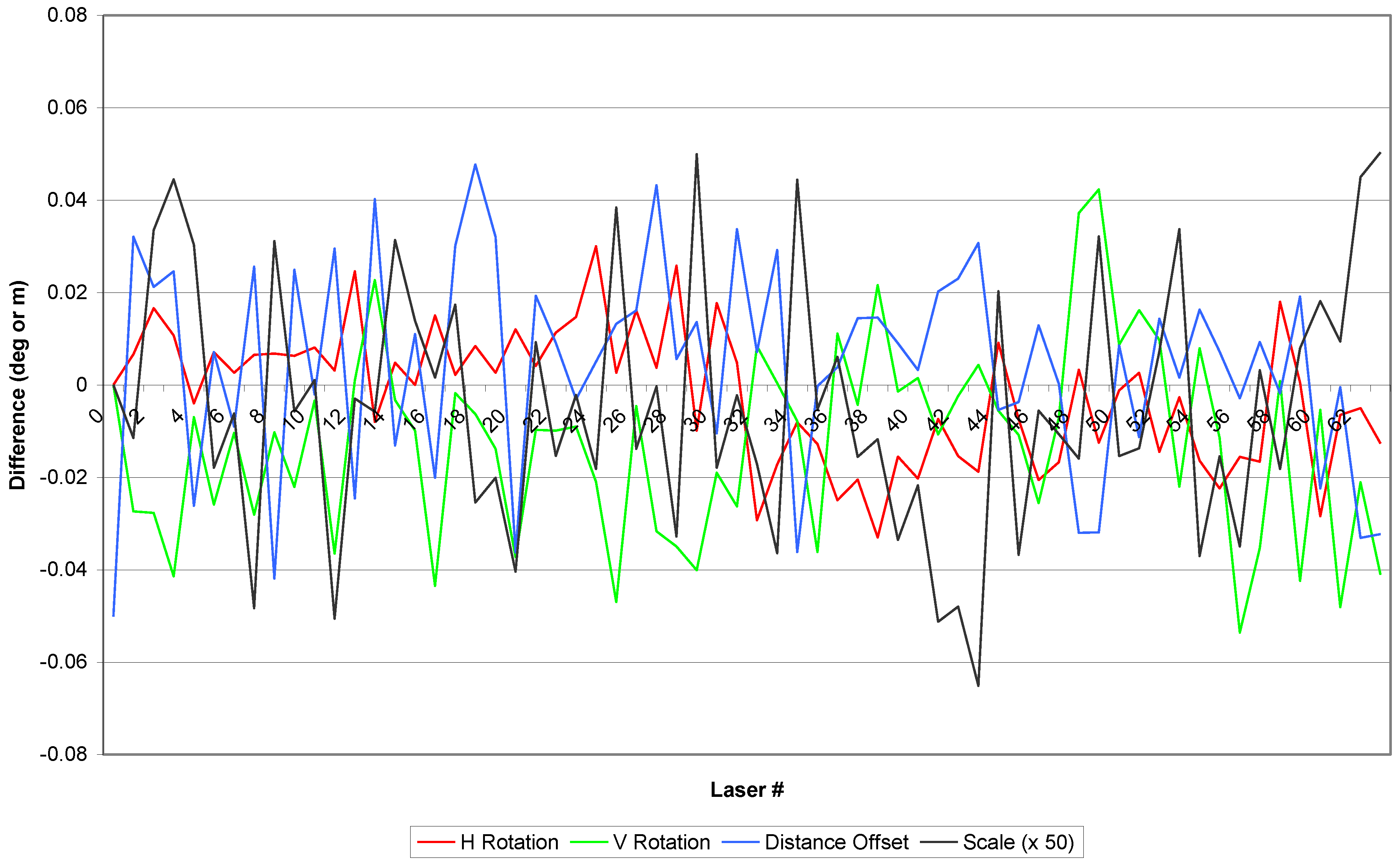
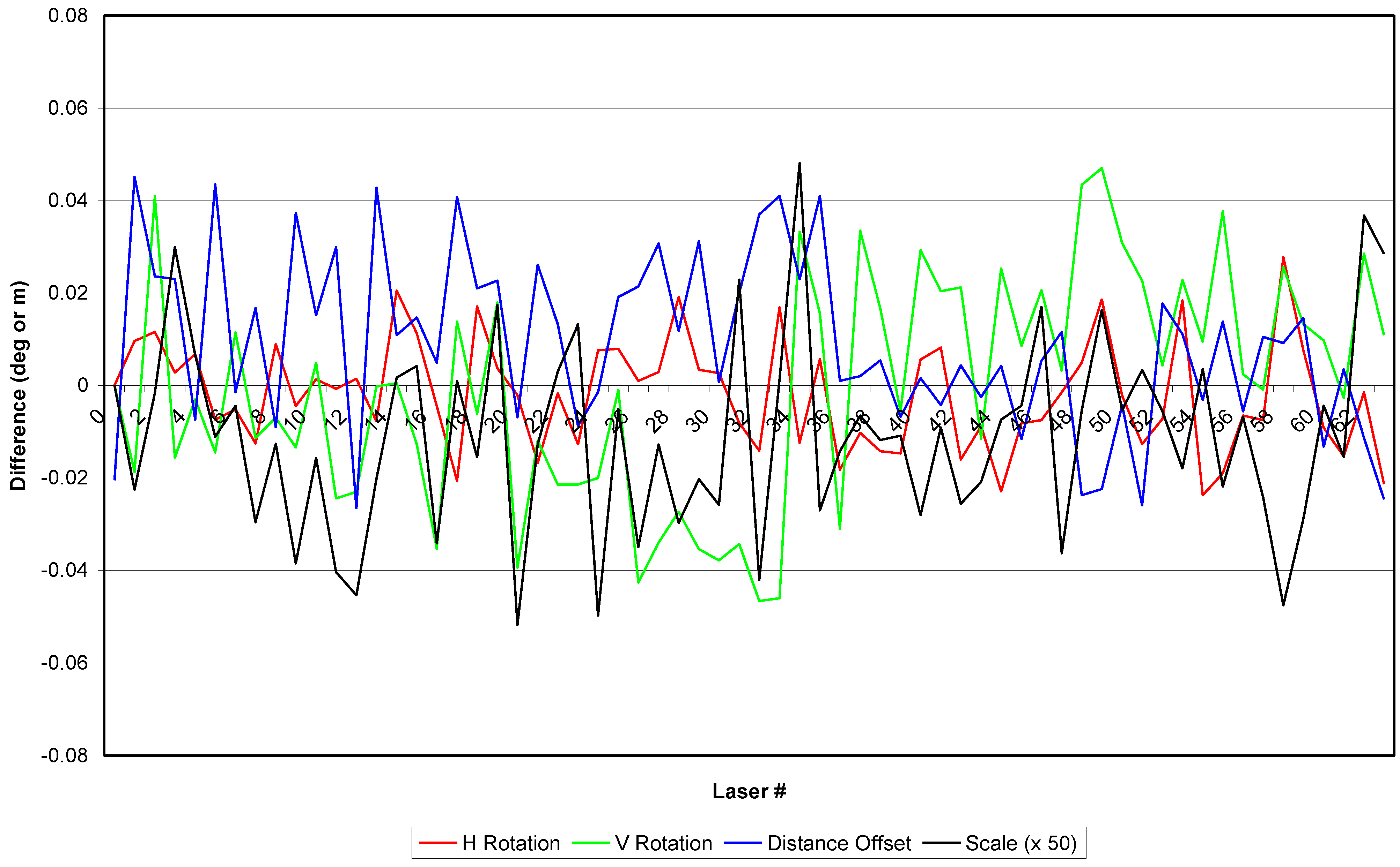
Figure 5 shows the difference in calibration parameters between Laser 1–Set 1, and Laser 1–Set 2, and
Figure 6 shows the differences between Laser 2–Set 1 and Laser 2–Set 2. Note that in
Figure 5 and
Figure 6 the scale factor difference has been multiplied by 50 to give an indication of the relative size of the scale differences. Fifty was chosen because it represents the longest raw ranges observed in the calibration datasets.
Figure 5.
Temporal Calibration Differences between Observation Sets for Laser 1.
Figure 5.
Temporal Calibration Differences between Observation Sets for Laser 1.
Figure 6.
Temporal Calibration Differences Between Observations Sets for Laser 2.
Figure 6.
Temporal Calibration Differences Between Observations Sets for Laser 2.
Overall, the temporal stability of the calibration shows a disagreement that is slightly higher than expected. Given that the stated range accuracy of the lasers is 2 cm (1σ), and the quantization noise on the encoder is 0.024°, we would expect agreement between epochs to be nearer to 0.02 (° or m) for all lasers.
A closer examination of the graphs shows that for all lasers, the agreement between the horizontal encoder offset is within the quantization noise of the encoder, which indicates a strong solution. However, the range offset, scale factor and vertical angle measurements all show disagreements up to the level of 4 to 5 cm in some cases (for the vertical angle, consider that 0.05° (= 4 cm at 50 m range). The differences in these three estimated calibration parameters will of course be largely determined by instability in the ranging accuracy of the lasers. Therefore, in an attempt to explain these errors the individual laser range measurements and their long term stability are examined.
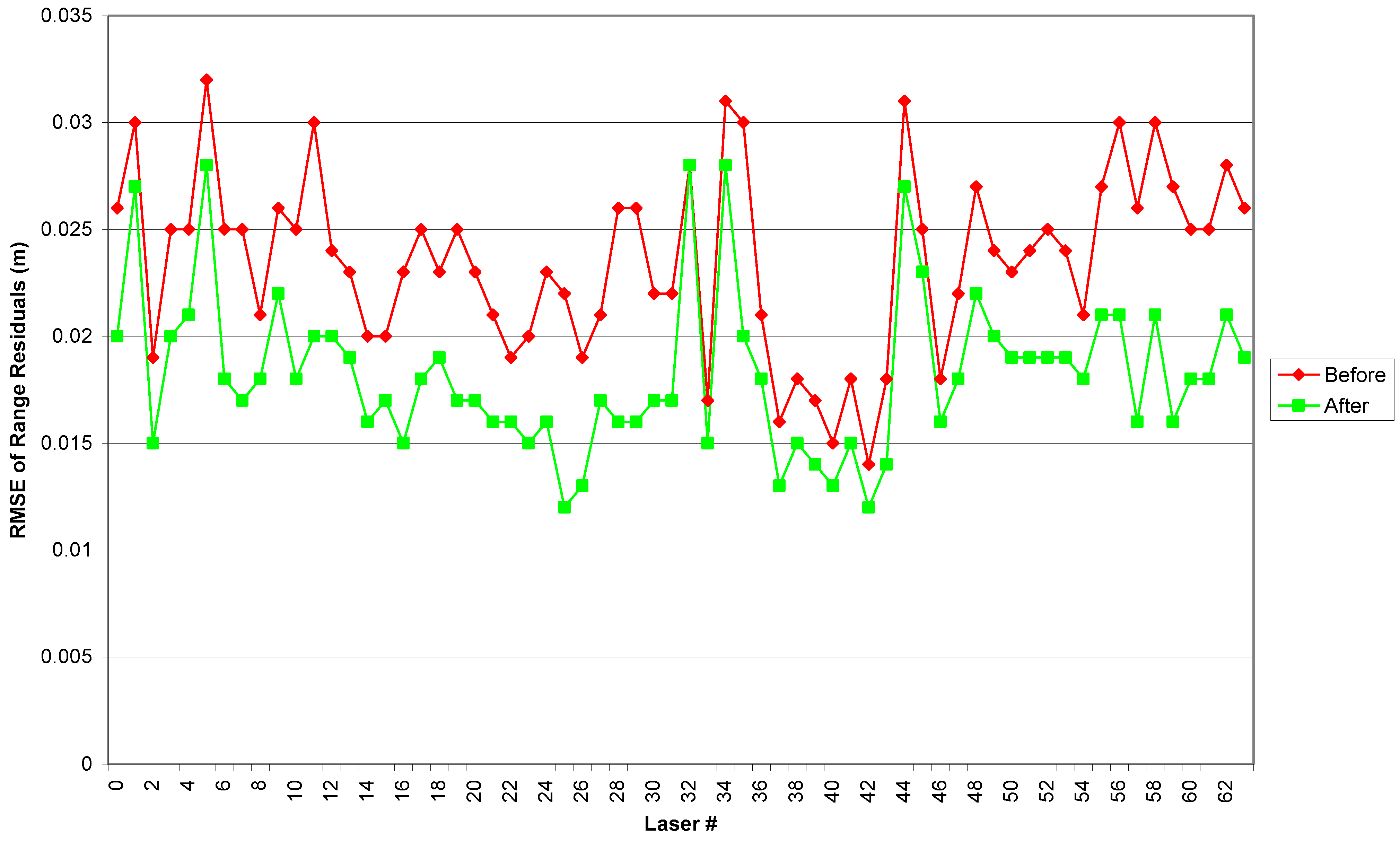
Figure 7 plots the RMSE residuals for each laser individually, before and after adjustment for Laser 2–Set 1. The figure clearly shows that there is an overall reduction in the RMSE range residuals for all of the lasers. However, even after adjustment, the residuals vary widely from laser to laser, from a minimum RMSE of 12 mm, to a maximum of 28 mm. For the purposes of the least squares adjustment however, all lasers were weighted equally. It is therefore possible that some of the higher than expected variability between epochs may be a result of the higher than expected residual noise in some of the lasers, although it is doubtful that this could be the cause of the majority of the variation in
Figure 5 and
Figure 6. However,
Figure 7 is an important by-product of the adjustment process. It allows an examination of each laser on an individual basis. For post-acquisition processing, the results in the figure could be used as a relative weighting scheme, or for high accuracy applications, the lasers with the worst performance (
i.e., 1, 5, 32, 34, and 44) could be eliminated from the final point cloud.
Figure 7.
RMSE of Range Residuals for Each Laser, Before and After Adjustment, Laser 2–Set 1.
Figure 7.
RMSE of Range Residuals for Each Laser, Before and After Adjustment, Laser 2–Set 1.
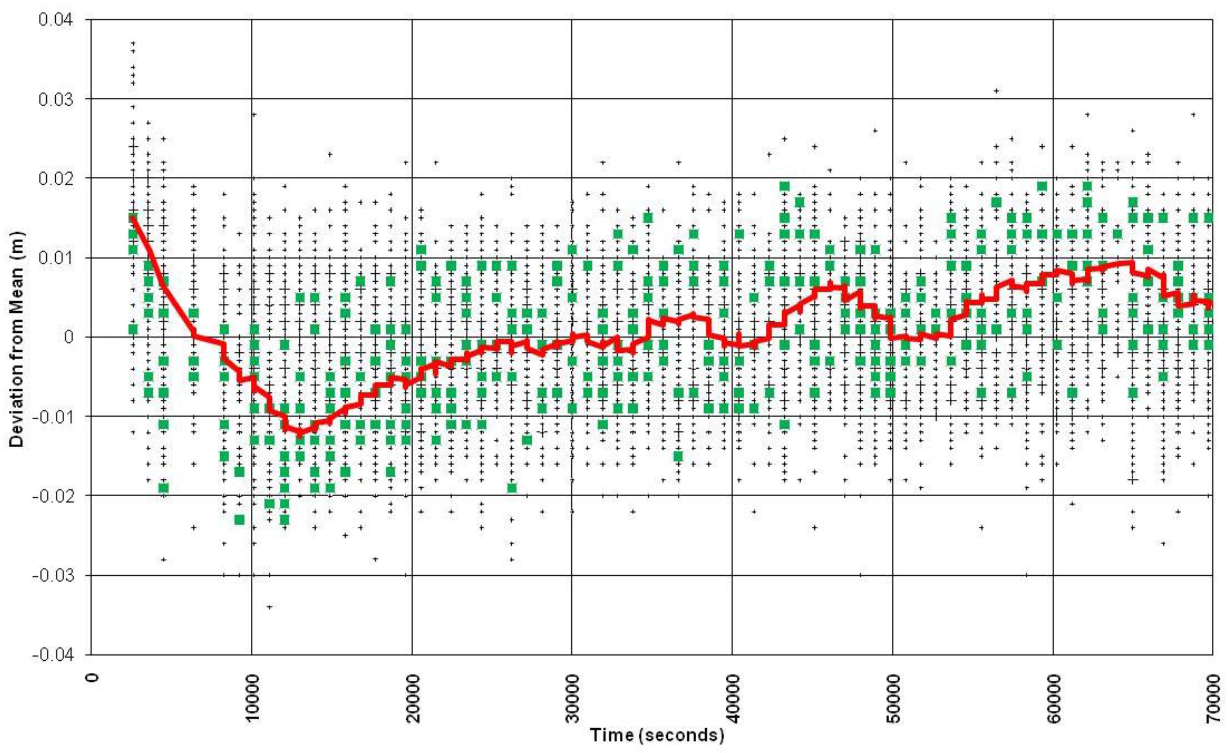
Based on the above comparisons, it is evident that there may be some longer term variations or problems with the accuracy of the individual range measurements. Therefore, in an attempt to discover the root cause of the problem, longer term static scans were collected from the scanner. The unit was set up to scan a wall at a distance of approximately 2.5 m. Ranges were sampled approximately every minute for a period of 18 hours. The initial dataset is shown in
Figure 8. Note that in the figure, the deviations from the average range taken over the entire dataset (for each individual laser) are plotted. Each laser is plotted individually, 63 lasers as black crosses, and one laser as green squares to show the representative deviation for a single laser. The red line in the Figure highlights the long-term average trend for all lasers.
In examining
Figure 8 it is apparent that there is not a significant long-term range drift in the instrument. The long term variability appears bounded by approximately ±2 cm, which is still within the ranging accuracy of the individual lasers. However, the one area of concern is the initial slope of the range biases on the left hand side of the graph, which shows a change in the mean bias of approximately 3 cm over a period of 3 hours. All of the datasets collected with the Velodyne for the purposes of this analysis were collected with 3 hours of turning the laser on. This would indicate that initially there may be some “warm-up” changes in the behavior of the sensor which may partially explain the higher-than-average differences in the temporal calibration parameters displayed earlier. Repeated static tests of the scanners have confirmed the behavior displayed in
Figure 8. Theoretically, this problem could be addressed by first allowing the scanner a warm up period. However, given that the period of warm up appears to be almost 3 hours, this would not be practical for either (a) calibration of the instrument or (b) using of the instrument on a mobile scanning platform.
Figure 8.
Long Term Range Drift—Velodyne HDL-64E S2.
Figure 8.
Long Term Range Drift—Velodyne HDL-64E S2.
8. Final Calibrated Residuals
As a final analysis of the temporally collected datasets, average calibration values were determined for both Lasers 1 and 2 from the adjusted calibration values determined with their respective Set 1 and Set 2 solutions. The averaged calibration sets were then used to correct the original observations to determine the overall planar misclosures for each of the four collected datasets. The results are presented in
Table 4, which shows for each of the four observation sets the global planar misclosure statistics for (a) the original Velodyne factory calibration values (Factory Calibration), (b) the derived calibration values from that observation set only (Set Calibration), and (c) an averaged calibration values using an average of both sets from each laser (Averaged Calibration). Note that for all statistics, planar misclosure outliers larger than 4σ, for the final adjusted points have been removed from the calculations.
The results in
Table 4 show that the averaged calibration parameters for each laser give a marked performance improvement over the factory calibration parameters for all four datasets. Although the average calibration does not perform as well as the set calibration determined individually for each observation session, the improvement over the factory calibration is consistently above 25%. This improvement is significant for high accuracy mobile scanning applications.
Table 4 shows that with temporally averaged calibration parameters a 3D RMSE accuracy of approximately 2.0 cm can be obtained with the Velodyne HDL 64E S2. Of course, this performance could theoretically be significantly improved if the laser were calibrated on a mission to mission basis. While possible, it is likely not practical to perform this type of rigorous internal calibration adjustment for the laser for all datasets collected.
Table 4.
Planar Misclosures for Each Observation Set with Factory, Set and Averaged Calibration Parameters.
Table 4.
Planar Misclosures for Each Observation Set with Factory, Set and Averaged Calibration Parameters.
| | Factory Calibration | Set Calibration | Averaged Calibration |
|---|
| | Min (m) | Max (m) | RMSE (m) | Min (m) | Max (m) | RMSE (m) | Min (m) | Max (m) | RMSE (m) |
| Laser 1–Set 1 | −0.170 | 0.123 | 0.025 | −0.061 | 0.060 | 0.015 | −0.076 | 0.075 | 0.019 |
| Laser 1–Set 2 | −0.135 | 0.181 | 0.029 | −0.051 | 0.051 | 0.013 | −0.076 | 0.074 | 0.019 |
| Laser 2–Set 1 | −0.184 | 0.170 | 0.026 | −0.052 | 0.052 | 0.013 | −0.079 | 0.081 | 0.020 |
| Laser 2–Set 2 | −0.160 | 0.224 | 0.028 | −0.048 | 0.048 | 0.012 | −0.080 | 0.081 | 0.021 |
9. Summary and Future Work
The analysis contained herein is built upon the initial static calibration analysis of the HDL 64E S2 which was reported in [
5]. First, the mathematical model of the Velodyne scanner was examined in more detail. Global misalignment terms, which represent deviations of the horizontal encoder from the vertical axis of scanning, were included. It was found that for the instruments examined in this study the misalignment is marginally significant, but should be monitored for additional scanner calibration computations before general conclusion about their inclusion in the mathematical model can be drawn. The horizontal and vertical offset parameters were shown to be very highly correlated with the horizontal and vertical angular offsets for the scanner, and they do not appear observable in any contrived static calibration observation scenario. It was therefore recommended that the manufacturer values for these parameters be treated as fixed.
Finally, the temporal stability of the scanner was examined by collecting observations with two separate HDL-64E S2 laser scanners, each with two observational data sets collected at two different epochs. For both scanners, the temporal agreement of the horizontal angle offset was at or near the quantization level of the encoder, however the vertical angle offset, distance offset and distance scale factor showed temporal differences that were larger than expected. Currently, we believe this is due to long term variability in the range measurements from the individual laser scanners, especially during their initial switch-on warm up period. However, despite this, an averaged (temporally) calibration set still showed a 25% or greater improvement in overall 3D planar misclosure over the factory determined calibration parameters. The final 3D accuracy of the observed point clouds was estimated to be 2.0 cm.
There are still some small additional temporal variations present in the point clouds whose root cause has yet to be identified, however the improvement in overall accuracy by removing these variations is not expected to be significant (perhaps 5 mm RMSE). As a final step, the authors plan to examine kinematic data collected with the Velodyne scanner and a navigation grade GNSS/INS unit to determine overall accuracy of the scanner for integrated high accuracy mobile mapping applications.


