1. Introduction
Across their range, native mountain goat (
Oreamnos americanus) populations have decreased over the last several decades [
1,
2]. In the Washington Cascades, some population estimates suggest declines of as much as 70% over the last 40 years (Washington Department of Fish and Wildlife unpublished data). Population declines and a re-evaluation of harvest potential for this species [
3,
4] have resulted in a reduction of harvest across Washington and has prompted research into the status of this unique ungulate [
5]. Conservation and recovery of mountain goat populations depends upon an understanding of habitat use [
6]. Therefore, we developed habitat models based on data from mountain goats fitted with Global Positioning System (GPS) collars in the Washington Cascades.
Application of GPS telemetry collars allowed for an unheralded opportunity to track mountain goats throughout the lengthy winter, a critical time period for survival, at a time when traditional telemetry and observational studies have substantial limitations. Although GPS telemetry has increased the number of locations collected on an individual animal by orders of magnitude over traditional radio tracking, GPS receivers may fail to acquire a position under forest canopies or when topography blocks satellite signals [
7]. Consequently, data from GPS-collared wildlife is biased toward areas of favorable GPS reception [
8,
9,
10,
11,
12]. We expected the GPS bias problem to coincide with habitats typical of those used by mountain goats during the winter. In the Cascades, mountain goats move to lower elevations during the winter [
13] where forest canopies tend to increase in both height and structure. Thus, the GPS bias problem was most likely apparent in the time period of greatest interest for developing an understanding of habitat use and the distribution of mountain goat habitat.
Our primary objective was to map resource selection probability functions (RSPF) [
14] at the 2nd order (home range) of habitat selection [
15] for annual, summer and winter time periods while increasing the resolution and accuracy of habitat models over previous efforts [
16]. Our secondary objective was to incorporate and critically evaluate a GPS bias correction factor. To account for the GPS bias, we developed, applied and evaluated a sample weighting factor based on stationary collar testing for the entire mountain range. The resulting habitat models provided information about the effectiveness of GPS bias correction and the distribution of potential mountain goat habitat in the Washington Cascades. Our models and maps contribute to more effective management and conservation of mountain goats in the Cascades and an example of the widest application of a GPS bias correction model to date.
1.1. Study Area
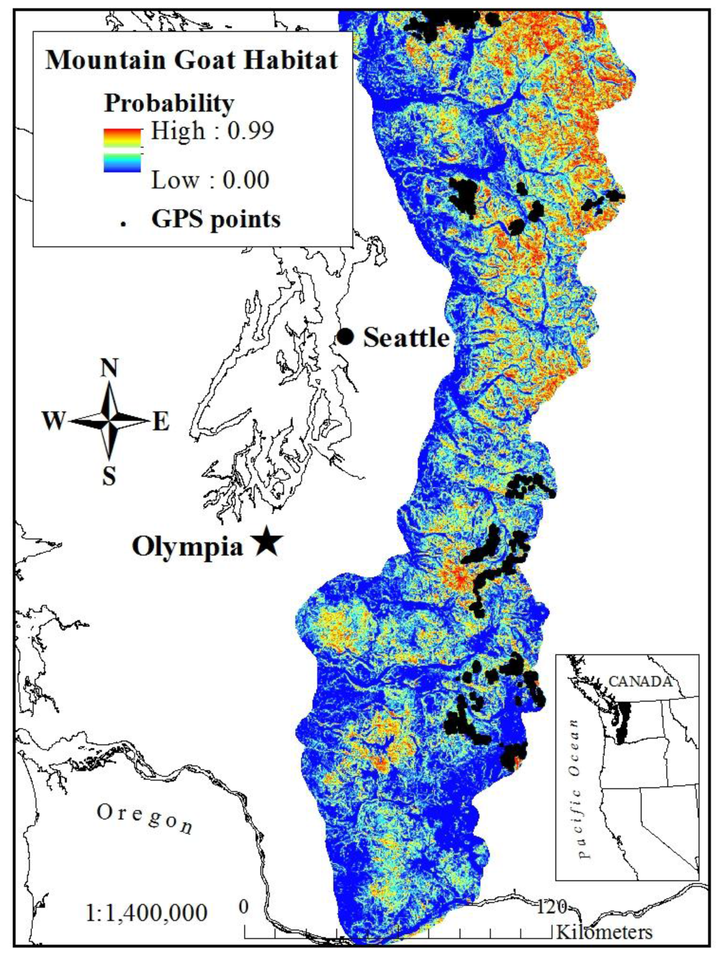
The study spanned the Washington Cascades (45.6°N to 49.0°N and −122.0°W to −120.0°W) and was divided into two distinct parts, habitat modeling and bias correction. The habitat modeling portion of the study focused solely on the Western Cascades (WC; 2.7 million ha;
Figure 1). The bias correction model covered both the WC and the Eastern Cascades (EC; 2.6 million ha;
Figure 2), naturally divided by the Cascade crest. The spatial extent (
Figure 2) of the WC and the EC was defined by the digital product distributed by the Inter-Agency Vegetation Mapping Project (IVMP) [
17,
18]. We expected to expand the habitat modeling to cover the EC and therefore developed the bias correction model to cover the expected range of mountain goat habitat present in the EC.
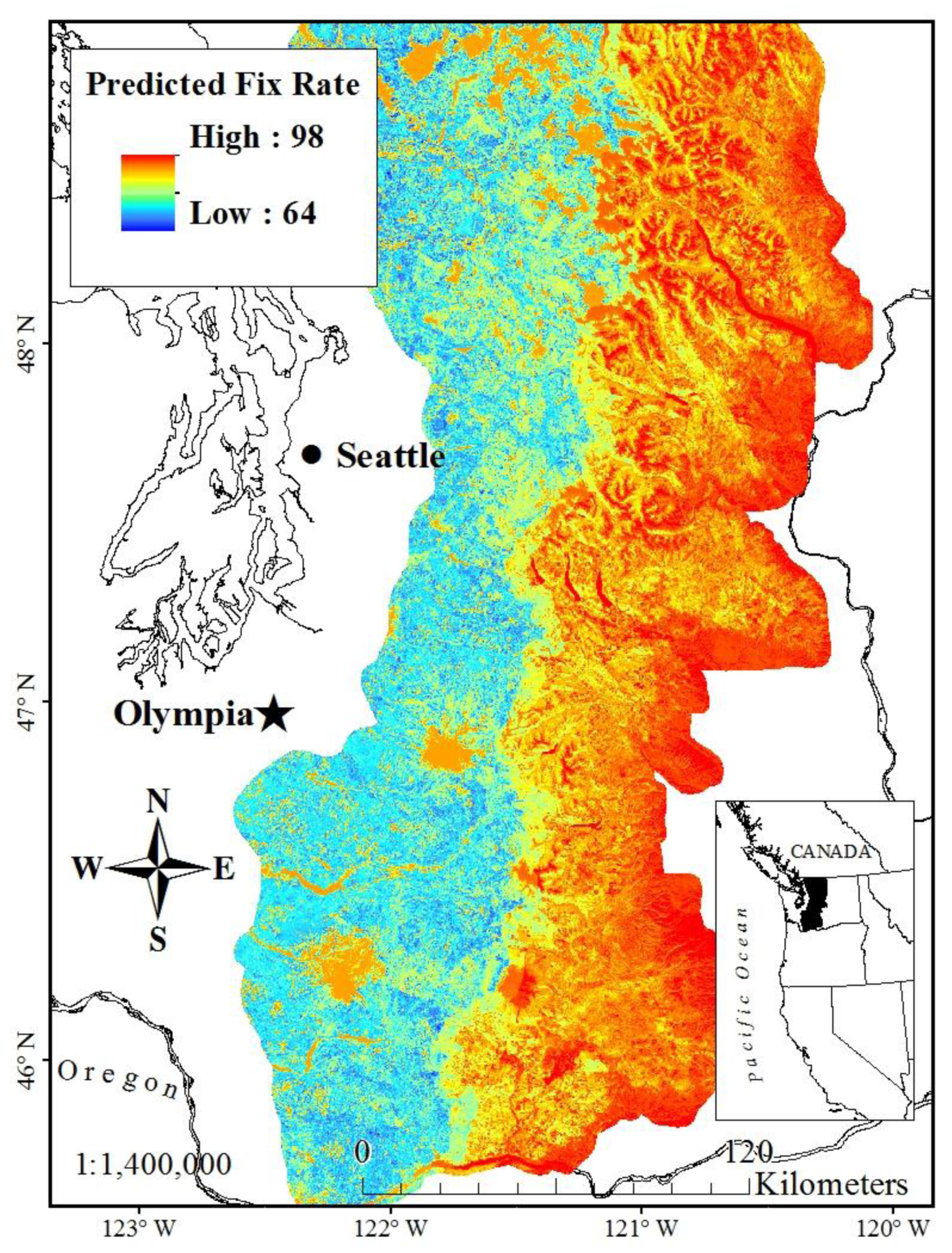
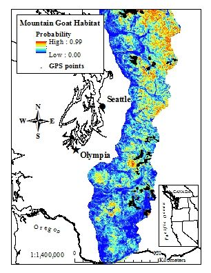
Figure 1.
Annual model of mountain goat habitat derived from a resource selection probability function (RSPF) in the western Cascades of Washington, USA (2003–2005) accounting for GPS bias (GPS locations from 38 mountain goats shown for reference).
Figure 1.
Annual model of mountain goat habitat derived from a resource selection probability function (RSPF) in the western Cascades of Washington, USA (2003–2005) accounting for GPS bias (GPS locations from 38 mountain goats shown for reference).
Mountain goats are native to the Cascade Range occurring both in the WC and the EC. The landscape of the Cascades is characterized by mountainous terrain with massive amounts of topographic relief, numerous glaciers and structurally diverse forest communities. The major ecological zones occurring in the study area included the montane, subalpine and alpine zones. The combination of physical and vegetative characteristics found in these ecological communities (ranging from dense forests in narrow valleys at lower elevations to treeless ridgelines) provided a wide range of conditions for testing GPS acquisition.
Figure 2.
GPS Position Acquisition Rate (PACQ) bias correction layer, based on stationary field sampling (2004–2005), across the western and eastern Cascades of Washington State, USA, used for sample weighting of GPS fixes from mountain goats.
Figure 2.
GPS Position Acquisition Rate (PACQ) bias correction layer, based on stationary field sampling (2004–2005), across the western and eastern Cascades of Washington State, USA, used for sample weighting of GPS fixes from mountain goats.
In the WC, the Pacific silver fir/western hemlock (
Abies amabilis/Tsuga heterophylla) forests are the most common forest community at lower elevations. Common associate over-story species included: Douglas-fir (
Pseudotsuga menziesii), Red alder (
Alnus rubra), and Western red cedar (
Thuja plicata). At higher elevations, Subalpine fir (
Abies lasiocarpa), Alaska-cedar (
Chamaecyparis nootkatensis), and Mountain hemlock (
Tsuga mertensiana) occur. In the EC, Ponderosa pine (
Pinus ponderosa) dominates the landscape. Common associates included Douglas-fir, Engelmann spruce (
Picea engelmannii), Subalpine fir, Western larch (
Larix occidentalis) and Lodgepole pine (
Pinus contorta) [
19].
2. Methods
2.1. GPS Bias Correction
We followed the experimental design proposed by Frair
et al. [
10] and adopted by Hebblewhite
et al. [
20] and Godvik
et al. [
21] to develop a model to predict the GPS position acquisition rate (
PACQ) based on testing stationary GPS collars for use in sample weighting. During 2004–2005, we benchmarked [
22] and tested 24 of the GPS collars that we eventually put on mountain goats. We stratified our sampling based on a range of environmental factors derived with a GIS that we believed
a priori might influence
PACQ in the WC and EC (
Table 1). We stratified our sample sites to cover the majority of combinations of the GIS variables that existed in the WC and EC and compared field measurements with the digital database with a simple correlation. To ground-truth the GIS variables, we recorded elevation (
R = 0.92), slope (
R = 0.60), aspect (
R = 0.56), and percent canopy cover (
R = 0.37) estimated with a spherical densiometer at each sample site.
Table 1.
Strata used for field sampling of GPS bias correction across the Washington Cascades during 2004–2005 based on the Interagency Vegetation Mapping Project (IVMP) data sets.
Table 1.
Strata used for field sampling of GPS bias correction across the Washington Cascades during 2004–2005 based on the Interagency Vegetation Mapping Project (IVMP) data sets.
| Variable | Description | Range of Values |
| Forest type (%) | Open | TVC < 30 |
| Semi-open | 30 ≥ TVC < 70 |
| Conifer | TVC ≥ 70, CC ≥ 70 |
| Mixed | TVC ≥ 70, CC and BC ≤ 70 |
| QMD(cm) | Western Cascades | 0–30 |
| 31–60 |
| 61–190 |
| Eastern Cascades | 0–25 |
| 25–190 |
| Slope and aspect (°) | Flat | slope < 20 |
| Steep north facing slopes | slope > 20 and aspect > 270 or < 90 |
| Steep south-facing slopes | slope > 20 and aspect > 90 and < 270 |
| Sky Visibility (%) | High | 0–60 |
| Intermediate | 60–70 |
| Intermediate | 70–80 |
| Low | 80–100 |
All sample sites were located near existing trail networks due to logistic constraints imposed by rugged and inaccessible terrain. Sample sites were >800 m in elevation and spaced ≥200 m apart. We secured GPS units approximately 1 m above ground with bamboo tripods or natural materials found on site. Site selection focused on areas with uniform vegetation characteristics within 30–50 m of the GPS units. We did not attempt to model potential edge effects or fragmentation of forest structure on PACQ due to the increased complexity of modeling a heterogeneous landscape without first understanding the effects of a homogeneous landscape. Furthermore, sites near the edge of a forest or alpine meadow could have resulted in differences between actual site conditions and the GIS data. We chose areas of uniform vegetation to focus the modeling process on areas that had the greatest chance for discerning the effects of vegetation on PACQ.
The GPS collars were programmed to attempt a fix for up to 3 minutes every 30 minutes for no less than 24 hours [
10] with a maximum acceptable positional dilution of precision (PDOP) 48.6 and an elevation mask of 5° above the horizon, beneath which GPS signals were ignored (Schulte, Vectronic‑Aerospace GmbH, personal communication). We defined the sample site position as the average position from all successful fixes. We calculated
PACQ as the percentage of fix attempts that were successful including both 2D and 3D fixes to avoid introducing extra bias [
23]. We screened for improbable GPS fix rates (GPS fix rates < 10%) due to suspected collar malfunction or disturbances to the sample site and restricted our analysis to the first 24 hours of data collection at each sample site.
2.2. GPS Bias Correction Variables
We extracted topographic and vegetation predictor variables at 2 spatial resolutions to model
PACQ. We extracted data for a single 25 m × 25 m pixel and for a 3 pixel by 3 pixel, or 75 m × 75 m square window centered over the pixel that contained the GPS sample site. These two data sets enabled us to examine the relationship between GPS performance and site conditions at two spatial resolutions. We derived topographic predictor variables from a 10 m digital elevation model (DEM) masked to the spatial extent of the IVMP data and resampled to 25 m. We created slope, aspect, sky visibility [
11,
23,
24,
25] data layers.
Vegetation variables for modeling
PACQ were derived from the IVMP data sets [
17,
18]. The IVMP data set consists of 4 data layers distributed as continuous variables: total vegetation cover (TVC), conifer cover (CC), quadratic mean diameter (QMD), and broadleaf cover (BC). QMD is defined as the diameter at breast height of a tree with the mean basal area of the stand. The IVMP provides these layers as continuous variables, but recommends discrete categorization based on tradeoffs between accuracy and category size; as the number of categories decreases the accuracy increases [
17,
18]. We classified each vegetation layer based on the distribution of values from sample sites and followed IVMP guidelines on the number of definable classes [
17,
18]. We classified percent TVC, CC, and BC for both the WC and the EC into 3 classes: 0–60%, 60–90%, and 90–100%; 0–40%, 40–90%, and 90–100%; 0–10%, 10–20%, and 20–100%, respectively. We defined 5 QMD classes for the WC: 0 cm, 0–12.4 cm, 12.4–24 cm, 25–58 cm, and >58 cm. For the EC, we defined 3 QMD classes: 0 cm, 0–12.4 cm and > 12.4 cm. The difference in variable delineation between stratification and modeling was due to the resultant frequency distribution of observations after we completed field work.
To avoid colinearity, we defined 5 vegetation summary predictor variables (TVBC) based on TVC and BC for both the WC and EC. After perfunctory analysis, we found that among the vegetation variables, TVC and CC were highly correlated (r = 0.88). Additionally, we found that TVC was the sum of CC and BC for the majority of sites. We defined the 5 TVBC variables based on the following combination of TVC and BC: TVC (0–60), TVC (60–90) & BC < 10, TVC (60–90) & BC ≥ 10, TVC (90–100) & BC < 10, TVC (90–100%) & BC ≥ 10. In each candidate model, we only considered one of the vegetation variables representing forest type to avoid colinearity.
2.3. GPS Bias Correction Analysis
We used an information theoretic approach with generalized non-linear mixed models to model
PACQ as clustered binary responses [
26,
27,
28,
29,
30]. Fix attempts at each sample site were coded as successful or not and had the same predictor variables over the course of the entire sampling period. We selected a series of models
a priori for testing based on expected ecological relevance [
31] and performed model selection and fitting in two steps.
First, we used non-linear mixed modeling (PROC NLMIXED; SAS Institute Inc., Cary, NC, USA) for model selection by fitting the candidate models using the logistic link with a single Gaussian random effect at the site level. The NLMIXED procedure fit nonlinear mixed models by numerically maximizing an approximation to the likelihood integrated over the random effects. Therefore, the AICc scores derived from the procedure could be used in model selection and we used AICc scores to rank models for each spatial resolution. However, the procedure estimated parameters for the conditional models. Our primary interest was to derive marginal parameters that had a population‑averaged interpretation in the sense that the effect of the covariates was averaged across sites. The conditional models fitted by NLMIXED are equivalent to marginal models with the same covariates and a compound symmetry (CS) covariance structure [
32].
In the second step, we used SAS generalized linear mixed modeling procedure (PROC GLIMMIX) to estimate the equivalent marginal models. In addition, we also fit a set of marginal models with the same covariates, but with a first-order autoregressive (AR1) covariance structure. For each selected model, we compared the corresponding marginal models under CS and AR1 covariance structure. We did not use the information theoretic approach to compare the marginal models because this estimation method was not likelihood based.
For each model, we calculated the area under the receiver-operating curve (ROC) for repeated measures [
33]. We chose the spatial resolution with the greater area under the ROC [
34] for each region, and used the resulting parameter values for predicting
PACQ across the landscape. Finally, to evaluate the predictive power of the bias correction models, we randomly split both the EC and WC datasets, across all animals, into model testing subsets (25%) and model building (75%) and regenerated parameter estimates. We used parameter estimates created with the model building data to predict fix rates in our testing subsets and compared predicted fix rate values to the observed fix rates values at these sites by calculating a coefficient of determination (
) described by Menard [
35].
We used the top models from the optimum spatial resolution to generate a map of predicted GPS fix rates for the EC and WC. The WC and EC bias layer were mosaiced into a single map covering all of the Washington Cascades. We used ArcMap 9.0 Spatial Analyst raster calculator to map predict
PACQ based on Equation (1) [
10]:
where
PACQ is the probability of successfully acquiring a GPS fix,
ß0 is the intercept
ß1…
ßp are coefficient estimates for variables
X1...
Xp [
10,
29]. The final map of predicted
PACQ was then used as a weighting factor during the habitat modeling. Each fix from a GPS-collared goat was weighted by the inverse of
PACQ [
10]. In the subsequent habitat analysis (described below), we created habitat models without any weighting and with the scaled weighting factor to evaluate the GPS bias correction factor to assess the influence of the GPS bias correction and also tested the habitat models using data from 9 additional GPS-collared mountain goats that were not used in the development of the habitat models.
Theoretically, the sum of the weighting factor for all fixes should equal the number of attempted fixes. Because this was not true in practice, we scaled the weighting factor. We multiplied the original, “naïve” weight, derived from the PACQ layer for each telemetry location, by the ratio of the expected attempted number of fixes over the sum of the all the telemetry weights. In this way, the bias correction weighting factor was forced to sum to the total number of fixes we should have obtained from the mountain goats fit with GPS telemetry collars. To understand how the scaling of the weights influenced the results of the habitat models we created habitat models with scaled weights, naïve weights and no weighting using a subset of data (north Cascades). We compared parameter estimates among naïve weighted, scale-weighted, and un-weighted for seasonal and annual habitat models.
In addition to applying our bias correction factor to the mountain goat data, we applied the weighting factor to a “pseudo-habitat” analysis of data that we collected during the bias correction field sampling. At a number of sample sites, the GPS units were left out longer than the 24 hour time period of sampling and recorded additional data. These extra data were treated as hypothetical animal locations and models of habitat selection for this hypothetical situation were developed based on the observed GPS data (with some missing fixes), the expected GPS data (with no missing fixes) and the weighted GPS data. We examined parameter estimates for all the “pseudo-habitat” models in both the EC and WC to gauge how the weighting factor altered parameter estimates toward the expected results, or truth. We created parameter estimates for a single model that included the IVMP data (BC categorized into 3 classes) and a selection of the topographic predictor variables. We did not evaluate diagnostics of the “pseudo-habitat” analysis, since the a priori rationale for selecting models to test in an information theoretic approach would have been based on the sample sites stratification. We simply examined how closely the parameter estimates from the “pseudo-habitat” models created with weighted GPS data compared to model created with the observed GPS data and the expected GPS data.
2.4. Mountain Goat Capture and Collars
Mountain goats were captured via aerial and ground-based darting with 0.4–0.5 mL Carfentanil or 50–70 mg xylazine hydrochloride mixed with 0.15–0.25 mg of opiate A3080 and reversed with 3.0 mL Naltrexone or 4.0 mL Tolazine, respectively [
36]. Capture methods complied with Washington Department of Fish and Wildlife Policy on Wildlife Restraint or Immobilization. Captured individuals were fitted with GPS telemetry collars (GPS plus collar v6, Vectronic-Aerospace GmbH, Berlin, Germany) programmed to record a fix (3 min max on-time) every 3 hour for 2 yr. Subsequently, GPS data were downloaded remotely via a handheld UHF-receiver.
2.5. Mountain Goat Habitat Variables
We evaluated habitat selection by mountain goats at two resolutions. For each fix, we extracted data at a single resolution for inclusion in the habitat analysis by centering a 75 × 75 m (5,625 m
2 or 0.56 ha) window over the 25 × 25 m pixel containing the GPS telemetry location. We opted to use this extraction window recognizing that over the 3-hour GPS sampling interval, mountain goats likely selected habitats at a range of scales around the resolution of the available digital products used to describe vegetation, which was 25 m × 25 m (625 m
2 or 0.06 ha). We also expected this 75 m scale to be more realistic given the location error in the GPS data. We evaluated the location error of the GPS units using the 95% circular error probable (CEP) [
37].
We developed a series of predictor variables in ArcGIS 9.0 to describe the topographic characteristics of the study area that were relevant to mountain goat ecology. Mountain goats occur in areas that are close to escape terrain and rely on steep slopes, cliffs and escarpments to avoid predation [
2,
6,
38]. We therefore derived predictor variables from a 10-m digital elevation model (DEM). We calculated distance to escape terrain (D2ET) [
39] as the distance from the center of each 25-m pixel to the edge of the nearest pixel of escape terrain. We defined escape terrain as areas with slopes > 35° based on an average of previously reported values [
38,
40,
41,
42,
43,
44]. We also created elevation (ELEV) [
39], slope and standard deviation of slope (SLSD) layers. We created an aspect layer to evaluate potential differences in habitat selection based on thermal gradients [
39]. We used the cosine (ASPCOS) and sine (ASPSIN) of aspect, to test for mountain goats habitat selection along either a north-south or east-west axis because we expected thermal cover, forest type and snow depth differ primarily along these 2 axes [
38].
To assess the influence of vegetation on habitat selection by mountain goats, we defined vegetation variables based on the data layers from the IVMP [
17]. We recognize that the IVMP data was not the ideal candidate for assessing relevant features of mountain goat ecology; however, the IVMP provided the largest extent of any available digital product describing multiple characteristics of the vegetation across the entire mountain range. We created 6 classes of TVC: 0–20%, 21–40% (TVC2), 41–60% (TVC3), 61–80% (TVC4), 81–100% (TVC5) total cover, and areas classified as rock and ice (TVC6). We broke the QMD data layers into 4 classes: No cover, 0–30 cm (QMD1), 31–60 cm (QMD2), and 61–190 cm (QMD3). The CC layer was classified into 3 discrete categories: 0–30%, 31–70% (CC2) and 71–100% (CC3). We excluded broadleaf coverage (BC) from the analysis as we did not expect BC to contribute to selection patterns by mountain goats. The final vegetation variables used for model creation also included the number of pixels, or variety (VAR), classified into each of the TVC, QMD and CC classes for each square extraction window at the 75 × 75 m resolution.
2.6. Mountain Goat Habitat Analysis
We developed 3 temporal habitat models, yearly, winter and summer, based on the use-availability design (type II, sampling protocol SP-A) [
14]. We divided the study area into 2 geographic regions, north and south as divided by the US Interstate 90 corridor, a significant barrier to mountain goats [
45]. We determined seasons based on elevation shifts of individual mountain goats [
13]. We used Hawth’s Analysis Tools [
46] to generate a matching number of random points with mountain goat locations per individual. We bound the elevation limits of our analysis with a buffer of 25 m beyond the highest and lowest observed GIS elevations of a mountain goat GPS location. We used weighted logistic regression, with clustering for individual, and Akaike's Information Criteria (AIC) to select a model [
31]. Application of the methodology described above for dealing with serially correlated binary data failed to converge when executed with the mountain goat data. We therefore, modeled the probability of a mountain goat location (π) as a RSPF [
14] defined by Equation (2) where the sampling probabilities approach zero while ignoring autocorrelation
where:
We calculated parameter estimates for habitat models, based on a 75% subset of all the GPS data, reserving the other 25% for model testing. To differentiate between habitat and non-habitat along the 0–1 range of predicted probability (π), we determined the cut-point at which the habitat models correctly predicted more mountain goat locations than random locations [
34]. With the reserved data, we calculated the percent of the locations that had predictive probabilities greater than the cut-point. We recalculated parameter estimates for the models without the weighting factor to gauge the influence of the bias correction factors on parameter estimation and evaluated the resulting predicted probability for the reserved data.
We also obtained 2 years of additional GPS data, provided by the National Park Service (NPS), on the locations of 9 mountain goats fitted with Vectronic-Aerospace GPS collars in Mount Rainier National Park (MORA; n = 6) and the North Cascade National Park (NOCA; n = 3). These data were not used in the habitat selection model and were collected after the time period of data used in the habitat models. MORA falls within the extent of the southern region of our habitat model and NOCA falls within the north, thereby offering 2 opportunities to benchmark our models. We plotted the GPS locations of the 9 NPS mountain goats against our habitat model predictions and recorded the percent of fixes classified as in mountain goat habitat. We calculated the percent of correctly predicted mountain goat locations for the all the habitat models with and without the GPS bias correction factor.
4. Discussion
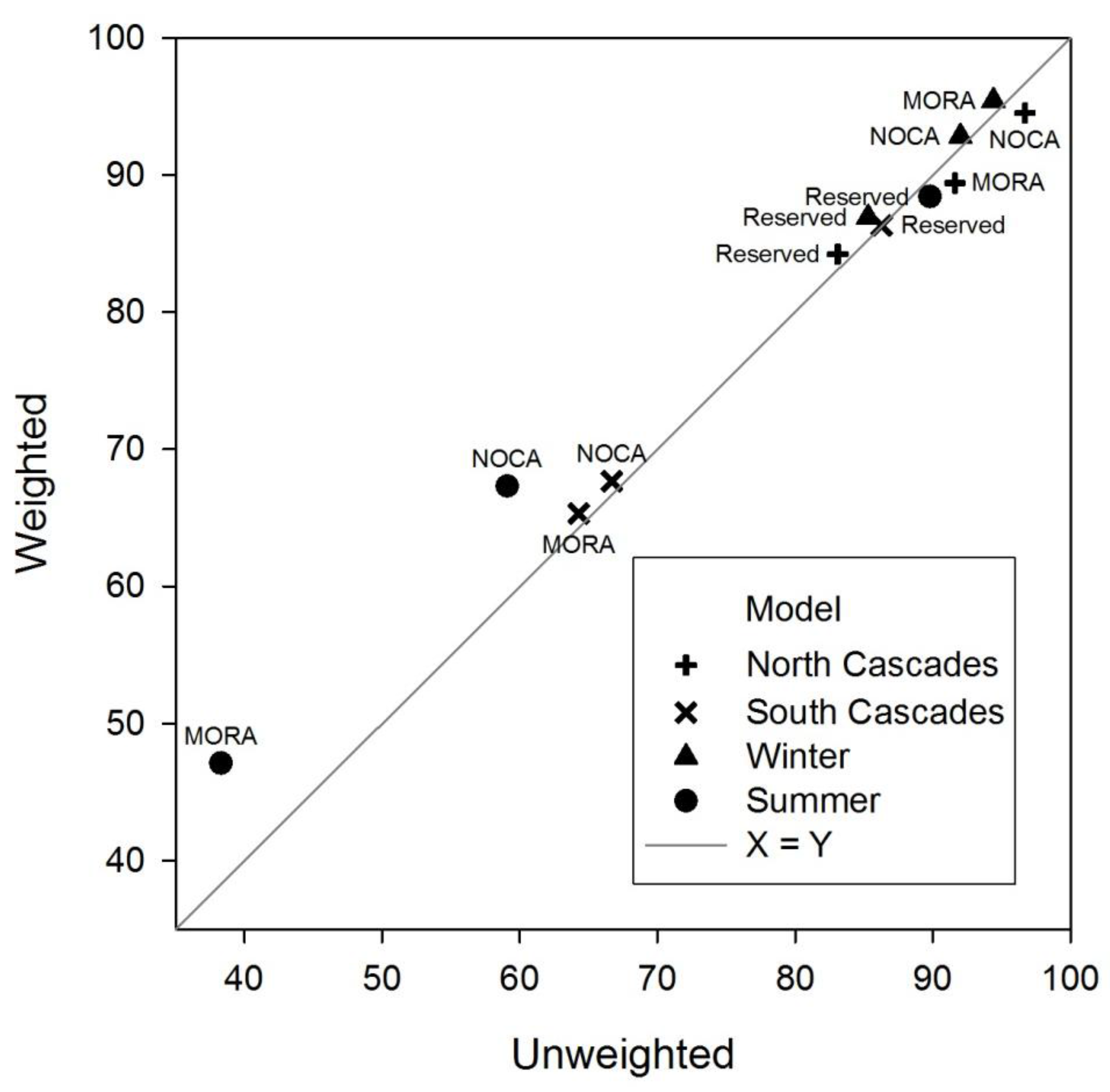
Overall, we expected a greater influence of the GPS bias correction factor on resources selection analysis and habitat prediction. When benchmarking the habitat models with testing data (25% of locations from study animals) the GPS bias corrected model performed slightly better than the uncorrected model. In 8 of 12 of the comparisons, the weighted habitat model had higher classification accuracies, although the difference was usually only 1–2% (
Figure 3). The greatest difference between habitat models created with and without the bias correction factor was about 8%, but was at the low end of overall classification accuracy. When the habitat models were benchmarked with the data collected from the 9 independent mountain goats, the uncorrected habitat models classified more mountain goat locations in what we described as mountain goat habitat than did the GPS bias corrected model. In addition to slight differences in validation accuracies between weighted and un-weighted models, there was little difference between parameter estimates of weighted
versus un-weighted models (
Table 5,
Table 6,
Table 7 and
Table 8). We found this to be the case in each of the comparisons between weighted and un-weighted models.
The lack of difference between the weighted and un-weighted models was unexpected and may be due to a number of factors. If the long-term temporal scale of the observed horizontal movements of mountain goats is fairly limited (no dispersal or long range movements) the amount of GPS data acquired may be enough to adequately characterize the selection of habitats in relation to availability. For example, if a mountain goat remained stationary for an extended period of time, even if the PACQ was quite low, the selection of that habitat would be constant as long as the number of available locations matched the observed number of locations. In other words, if only one cover type was actually utilized, then the number of observations acquired will not change the selection estimates. This would likely vary as a function of the movement and behavior of a mountain goat in relation to climatic factors (such as snow depth), the age, and sex of collared animals. In other words, the differences between PACQ among habitats may be negligible based on the behavior of the individual animal, the general ecological relationships of the species to the study area, and perhaps more paramount, the statistical method employed to address the research question of interest. In the future, understanding the consequences of data loss prior to beginning a GPS collaring effort will be helpful in understanding at what magnitude data loss will alter results of habitat analysis beyond acceptability for the question of interest.
Behavior has the additional compounding factor of influencing P ACQ. Our experimental design did not account for activity and this may be why our GPS bias trials had an overall higher PACQ than the mountain goat data. Presumably, the lower PACQ exhibited by the collar data depends in part on behavior and the interaction of behavior and habitat. For example, if an animal spends a great deal of time lying down (with the GPS antenna in suboptimal position) in habitats with otherwise good GPS signal reception and a great deal of time foraging in habitats with otherwise poor GPS signal reception, the interaction could result in no differences in PACQ among these habitats. Our GPS bias correction model was not designed to account for the variation of PACQ from mountain goat telemetry data due to activity.
It is also possible that our analysis was flawed in that the scale of the GIS data may not capture the actual environmental factors that influence acquisition of GPS satellite signals. Nevertheless, our model diagnostics were comparable to other published studies advocating this modeling approach. The goodness of fit of our GPS bias correction model was low to acceptable (WC:
= 0.296,
ROC = 0.70 and EC:
= 0.202,
ROC = 0.68) which was comparable to other studies that reported similar metrics. D’eon
et al. [
23] and D’eon [
47] incorporated canopy cover and available sky in a model with a fix rate
R2 = 0.229 whereas Lewis
et al. [
37] reported fix rate
R2 = 0.028–0.099 for models including sky visibility and canopy cover. Hebbelwhite
et al. [
20] reported the area under the
ROC = 0.81 for a model predicting the probability of obtaining a successful fix based on collar manufacturer, aspen, closed conifer, and topographic position in narrow valleys or steep slopes. Hebbelwhite
et al. [
20] also reported a range of ROC scores between 0.71 and 0.75 for models based on individual collar manufacturers. Frair
et al. [
10] reported an area under the
ROC of 0.683 for
PACQ based on a model including collar type, vegetation class, percent slope, and the interaction of slope and vegetation. Only Frair
et al. [
10], Hebbelwhite
et al. [
20] and our study accounted for the lack of independence betweensuccessive fixes at each trial site in their analysis. Even though we expanded upon the statistical approaches advocated in the literature to deal with binary data that is serially correlated and clustered, our habitat analysis showed little difference between models created with a bias correction factor
versus those created without a bias correction factor. Our study is the largest reported effort to correct for the GPS bias issues using the sample weighting approach. Our bias correction model included hundreds of sample sites and was applied across the widest geographic extent yet reported, but did not markedly change model predictions and improved predictions by only a few percent.
More studies are addressing how the GPS bias correction models actually influence the results of a habitat selection [
10,
21,
48]. Frair
et al. [
10] addressed the question of how bias correction changed the results based on 10 iterations of simulated 30% data loss based on
PACQ. Frair
et al. [
10] found that sample weighting reduced Type II error rates and corrected the coefficient bias. We found, like Godvik [
21], that our parameter estimates did not change in a meaningful or explainable manner in any of the comparisons we made including: among yearly models (both north and south), among seasonal models, among models scaled to correct for the expected number of telemetry locations we should have acquired, and among models with known selection ratios. Likewise our pseudo habitat analysis did not correct the biased parameter estimates back to the original, true estimates.
Despite the negligible differences between habitat models created with or without a GPS bias correction factor, the amount of telemetry data accrued allowed us to create habitat maps that performed well and matched with our expectations of the distribution of mountain goat habitat (
Figure 1). The habitat models however, suffer from some flaws. Notably, the modeling did not account for the lack of independence between successive GPS fixes from an individual mountain goat, nor were the vegetation data provided by the IVMP optimum for discerning mountain goat habitat. The habitat models however do not provide insightful ecological interpretations of habitat selection by mountain goats due to the number of variables included in the final models. Nonetheless, the resultant models, when displayed in a GIS provide a more detailed depiction of the habitat available to mountain goats in the western Cascades based on a large number of observations over the course of two years. In particular, the data acquired during the winter time provided the most comprehensive data set for analysis of habitat selection by mountain goats during this difficult study period. These data can assist with future management, conservation and research plans to meet the multiple goals of the numerous authorities and interest groups of the region.
The performance of our GPS bias correction model poses some questions and highlights additional avenues of research. If this approach to correct habitat induced GPS bias is to be continued, the foremost imperative of research needs to be a critical evaluation of how a GPS bias correction model and weighting scheme can produce an unbiased result. Further simulation studies, like those of Frair
et al. [
10] and Nielson
et al. [
48] are the most likely means of addressing the limitations and problems of this method. Such studies may clarify which variables in a GPS bias correction model have more of an influence on fix success rates and if the bias correction factor can adjust habitat selection estimates back to actual values obtained from real-world data. Simulation studies will also help understand the magnitude of the GPS bias correction problem in habitat analysis [
48]. More simulation exercises may help assess at what point, and to what extent, data loss alters parameter estimates of habitat selection models beyond some statistical threshold of significance or acceptability. The challenge remains however, to demonstrate correction of habitat coefficients from real-world data. When employing the stationary collar sampling design, the time interval should match those of collars deployed on wildlife [
12] and the influence of animal behavior on
PACQ needs to be addressed for the specific species of interest [
11,
49]. The decision to pursue a bias correction model in future studies by other researchers shouldn’t be ignored, but carefully consider in light of our results. We concluded that the weighted sampling approach yielded virtually no difference between bias corrected and un‑corrected results. If data loss is great enough based on initial returns from deployed collars, research may need to investigate the causes and implications (via simulation of habitat models based on differing rates of data loss) of the bias. If there is a high enough fix success, obviously the entire point is moot.
Our habitat models ignored the inherent autocorrelation of GPS data from wildlife. Application of the modeling technique we developed here to deal with the autocorrelation in the bias data resulted in a failure of the computer algorithm to converge when applied to the mountain goat data. Furthermore, the ecological justification for application of the methodology for dealing with the bias data does not necessarily apply to wildlife since successive locations from free roaming animals may have variable distances, times, and related predictor variables. The ongoing development of statistical and modeling techniques to capitalize on the lack of independence between successive GPS fixes from free ranging wildlife in habitat and space use studies [
50], will refine the ability to develop ecologically meaningful habitat models and to deal with the large amount of data accrued by GPS collars.


