Acquisition of Bidirectional Reflectance Factor Dataset Using a Micro Unmanned Aerial Vehicle and a Consumer Camera

Abstract

This paper describes a method for retrieving the bidirectional reflectance factor (BRF) of land-surface areas, using a small consumer camera on board an unmanned aerial vehicle (UAV) and introducing an advanced calibration routine. Images with varying view directions were taken of snow cover using the UAV. The vignetting effect was corrected from the images, and reflectance factor images were calculated using a calibrated white target as a reference. After spatial registration of the images using a corresponding point method, the target surface was divided into a grid, and a BRF was generated for each grid element. Lastly a model was fitted to the BRF dataset for data interpretation. The retrieved BRF were compared to parallel ground measurements. Comparison showed similar BRF and reflectance factor characteristics, which suggests that accurate measurements can be taken with cheap consumer cameras, if enough attention is paid to calibration of the images.

1. Introduction

Traditional satellite and manned aircraft-based remote sensing instruments have the advantage of covering large areas with good accuracy. However, the high expense of operating such instruments limits the availability of up-to-date information for specific areas of interest. For many applications more flexible, affordable and user-friendly local-area remote sensing systems are needed.

Unmanned Aerial Vehicles (UAV) are an affordable solution, filling the gap between manned aircraft- and ground-based measurements. When compared to traditional aerial remote sensing campaigns using helicopter or fixed-wing aircraft, UAV campaigns involve less preliminary planning and offer flexibility for the exact measurement time. Passive optical remote sensing is in many cases limited by the weather, and by using UAVs an optimal weather gap can be selected for the measurements.

With light UAVs, the drawback has been the limited payload capability and operation time. However, fast development in consumer cameras over recent years has brought lightweight and affordable cameras to the market. If enough attention is paid to the processing and calibration of the data [1,2], satisfying results can be achieved with these cheap sensors, even though consumer cameras are not comparable to the high-end aerial photography cameras.

One application for which UAVs are well suited is measurement of the sunlit bidirectional reflectance factor (BRF) [3,4], which describes the directional reflectance characteristics of a target surface. The BRF is determined by measuring the reflected radiance of the target surface from several directions and comparing those measurements to the reflected radiance of an ideal and Lambertian surface under equal illumination conditions. This data is usually measured using ground-based instruments, such as the Finnish Geodetic Institute Field Goniospectrometer (FIGIFIGO) [5,6]. Unfortunately, the ground-based measurements are usually limited to one small target, which often leads to problems in sample representativeness. With UAVs, the distance from the sample area can be significantly longer, and by using imaging instruments, a large area can be covered with one flight. With the help of onboard sensors, such as GPS and an electronic compass, modern unmanned aerial vehicles can autonomously carry out complex flight missions required for BRF measurements.

In this paper, a new automatic flying observation system concept, consisting of a Microdrone MD4-200 quadrotor UAV and a consumer digital camera, is introduced. BRF data has been measured, processed and validated, and the results are presented here with strong emphasis on the processing and calibration. Ideas for developing the data processing and measurements are discussed.

2. Instruments

2.1. UAV

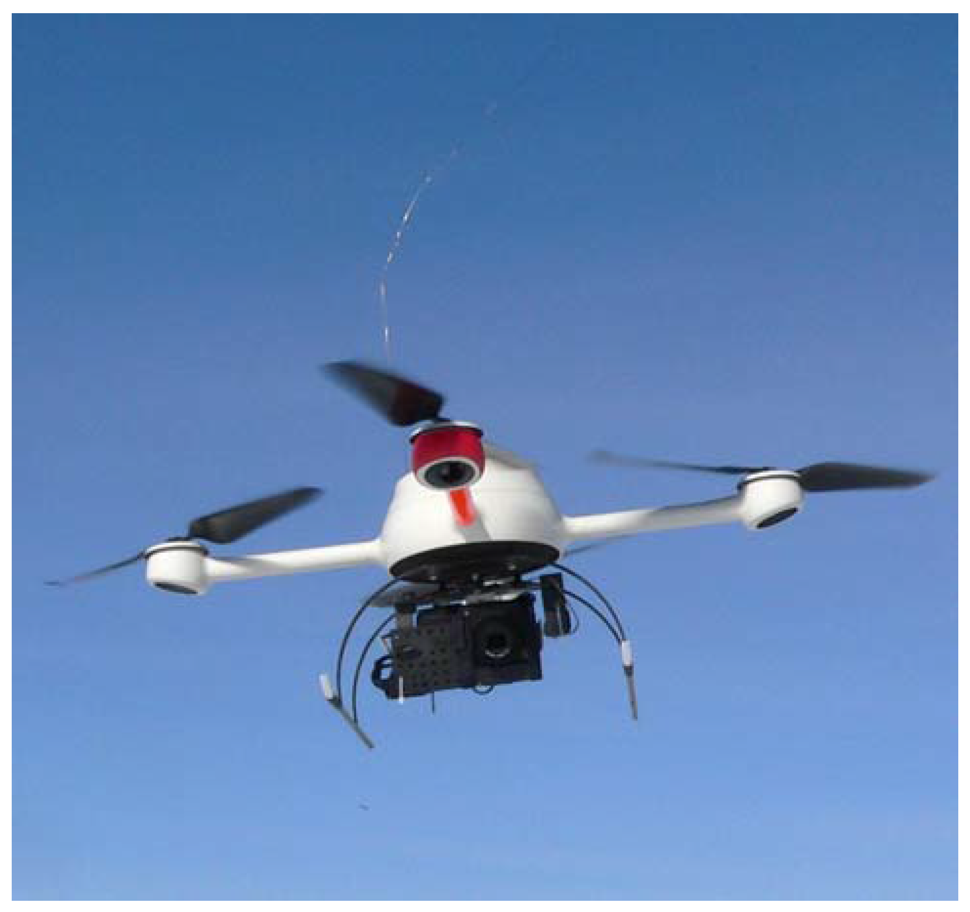
The UAV used is model MD4-200 (Figure 1), manufactured by Microdrones GmbH, Germany. It can take-off and land vertically from a small open area and has an onboard flight controller with a compass and inertial, gyroscopic, barometric and GPS sensors. The data recorded by these sensors is logged and can be accessed during post processing. Flight missions can be programmed to the UAV with a predetermined route and positions for taking measurements. The UAV is battery powered and has a flight time of 10–20 minutes, depending on the payload and weather conditions. A strong wind of over 4 m/s forces the UAV to use a high rotor rpm, draining the battery faster, and causing excessive shaking and motion blur to the images. Temperatures down to −20 °C do not have any effect as long as the batteries are kept warm. The UAV is rather small, being only 55 cm from side-to-side, and thus the payload limit is low, around 300 grams.

The UAV carries a small consumer camera, the Ricoh GR Digital II. It has a 10 megapixel 7.36 × 5.52 mm² CCD sensor with a pixel size of 2 × 2 μm², a 5.9 mm focal-length objective (equivalent to 28 mm for a 35 mm film camera), a manually adjustable F number from 2.4 to 11, a shutter speed of up to 1/2,000 s and the capability to save raw images with 12-bit color depth. The total weight of the camera is approximately 200 grams. The camera is mounted to a custom-built tilting platform underneath the UAV and can be triggered by the remote controller of the UAV or automatically by the onboard flight controller.

Figure 1. MD4-200 Unmanned Aerial Vehicle during snow measurements in spring 2009 with the Ricoh GR Digital II camera.

Figure 1. MD4-200 Unmanned Aerial Vehicle during snow measurements in spring 2009 with the Ricoh GR Digital II camera.

2.2. Ground Equipment

To validate the UAV results, ground based bidirectional reflectance factor measurements were taken using the Finnish Geodetic Institute Field Goniospectrometer (FIGIFIGO, Figure 2). The primary sensor of FIGIFIGO is an ASD FieldSpec Pro FR spectroradiometer, and other instruments include a pyranometer for measurement of the hemispherical illumination level, a fisheye camera for sun-direction determination, and an inclinometer to measure the sensor zenith angle. FIGIFIGO can measure the BRF of a target in 15 minutes with 20° azimuth and 5° zenith resolution in the 350–2,500 nm wavelength range.

The reflectance factor is measured as the ratio of reflected light from the target surface to reflected light from an ideal Lambertian reference target. For FIGIFIGO, a 25 × 25 cm² Spectralon panel was used as a reference. This was not large enough for UAV applications, and a commercially available fabric gray card, normally used for white-balancing cameras, was used as a substitute. The diameter of the fabric target is 50 cm, which was found to be enough for distances of approximately 50 meters. Unfortunately, the fabric has highly specular reflectance characteristics, especially at low illumination angles, making it a poor reference target for BRF measurements. For this reason, the BRF of the fabric was measured in the laboratory and corrected during post processing.

Laboratory facilities include a 1,000-watt stabilized quartz-tungsten-halogen lamp and an off-axis parabolic-mirror system that creates a collimated beam of 50 cm in diameter. During laboratory measurements, the illumination angle can be freely selected to represent the field measurement conditions. When the sample is illuminated with the desired geometry, FIGIFIGO is used to measure the BRF.

Figure 2. Left: Finnish Geodetic Institute Field Goniospectrometer (FIGIFIGO). Right: The measurement setup as seen from an aerial image. FIGIFIGO was turned around the sample area, the spectralon reference was measured before and after a sample measurement, and a pyranometer monitored the illumination level.

Figure 2. Left: Finnish Geodetic Institute Field Goniospectrometer (FIGIFIGO). Right: The measurement setup as seen from an aerial image. FIGIFIGO was turned around the sample area, the spectralon reference was measured before and after a sample measurement, and a pyranometer monitored the illumination level.

3. Measurement, Calibration and Processing

A flight mission has descriptions for flight altitudes, picture-capturing positions and directions, and flight speeds between the picture positions. With the BRF-measurement flights, all of the images had a common point of interest to which the images were centered. The UAV flew around this point and acquired images from various directions, with as wide a view-angle distribution as possible. The altitude during flights was 35–40 meters, and view angles up to 50° from nadir. The spatial resolution of the images was approximately 1–1.5 cm, depending on the altitude and view angle.

The reference targets were placed close to the center of the target area to make sure that they were visible in every image. The leveling of the reference targets is critical, because if the reference target is tilted toward or away from the direction of illumination, a large error arises in the measured reflectance factor. The weather during the flight was calm and clear. The camera settings were selected so that even the brightest objects in the image would not saturate, the focus of the camera was fixed to infinity, and all of the settings remained constant while measurements were being made.

Parallel ground measurements were taken with FIGIFIGO during the UAV flight. The illumination conditions remained stable, and therefore ground measurements were also taken before and after the flight. Samples similar to those found in the UAV target area were measured and used as a reference during post processing.

The images acquired with the small consumer camera of the UAV setup were not suited for analytical use without calibration. The radiometric repeatability of the camera was found inadequate for reflectance measurements, without a reference target in each image. Laboratory tests showed random variations of up to 5% in overall image intensity between images of a uniformly illuminated target, presumably due to inaccurate timing of the shutter. Vignetting causes the image corners to be approximately 25% darker compared to the center of the image, depending on the camera settings. The geometry of the camera was not calibrated, and large geometric distortions were observed. To correct all these issues, a processing chain similar to [1,2] was used.

3.1. Preparation of Images

Before further processing, the quality of the images was manually checked. An image was removed from the dataset if blurred or if it did not cover enough of the target area. While slight blurring did not make the image unusable for retrieving BRF data, it did cause problems in image registration.

When downloaded from the camera the images were in Digital Negative (DNG) format, and were converted to TIFF using a program called dcraw [7]. The raw images were Bayer-type color filter array files consisting of clusters of four pixels. Each cluster has one red, one blue and two green pixels. For further processing the pixels were separated to component images consisting only of pixels of the same color.

3.2. Flat-field Correction

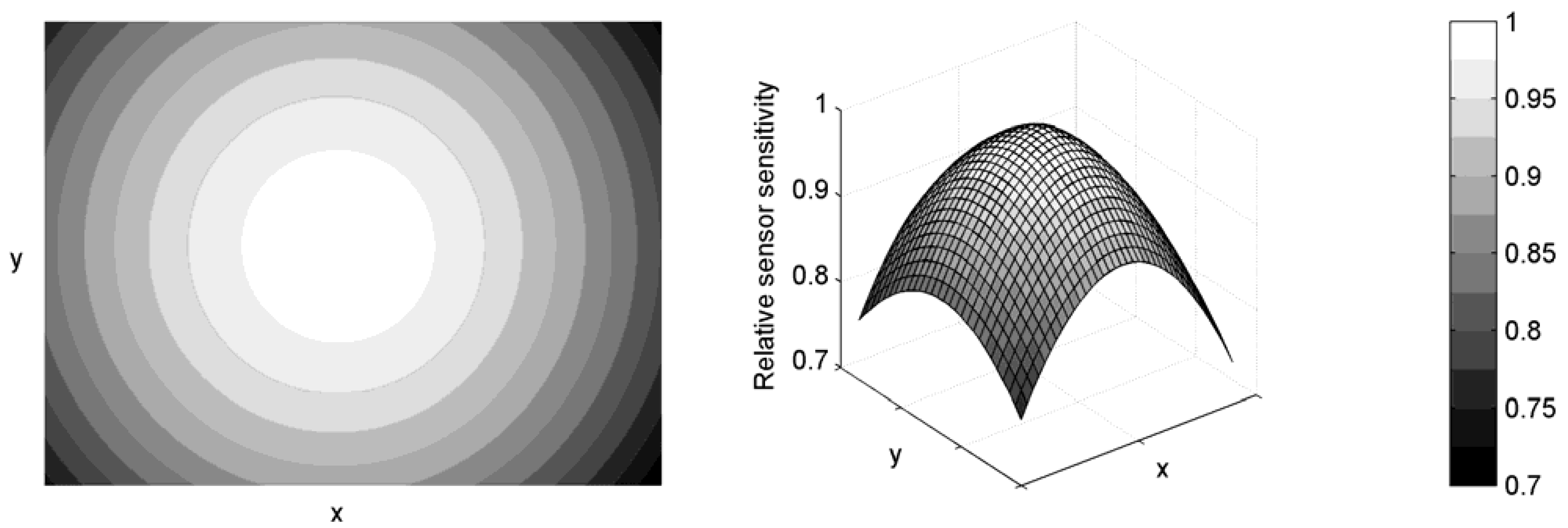
The dataset used for this experiment allowed a simple method for correcting the vignetting effect (Figure 3). All images were of uniformly illuminated white snow cover, with view directions varying so that some of the images are from the opposite direction to the others. With random view directions, the systematic BRF effects of the surface were mixed. Thus, when a mean image was calculated from all of the images, the BRF effects were smoothed out. However, due to the limited size of the dataset, this mean image still had some artifacts (trees, etc.) remaining from single images, which needed to be smoothed by fitting a model.

Figure 3. The flat-field calibration image. A large difference of around 25% in sensitivity is seen between the image center and the corners.

Figure 3. The flat-field calibration image. A large difference of around 25% in sensitivity is seen between the image center and the corners.

$$FF=a{r}^2+br+c+dx+ey$$

(1)

The model has three parameters (a, b, c) for a second degree parabola and two parameters (d, e) to take into account the inaccurate sensor position relative to the optics. r is the distance from the center of the image, and x and y are pixel positions on the corresponding axes. This simple model was found adequate in modeling the flat field with reasonable accuracy.

3.3. Image Reflectance Calibration Using a Reference Target

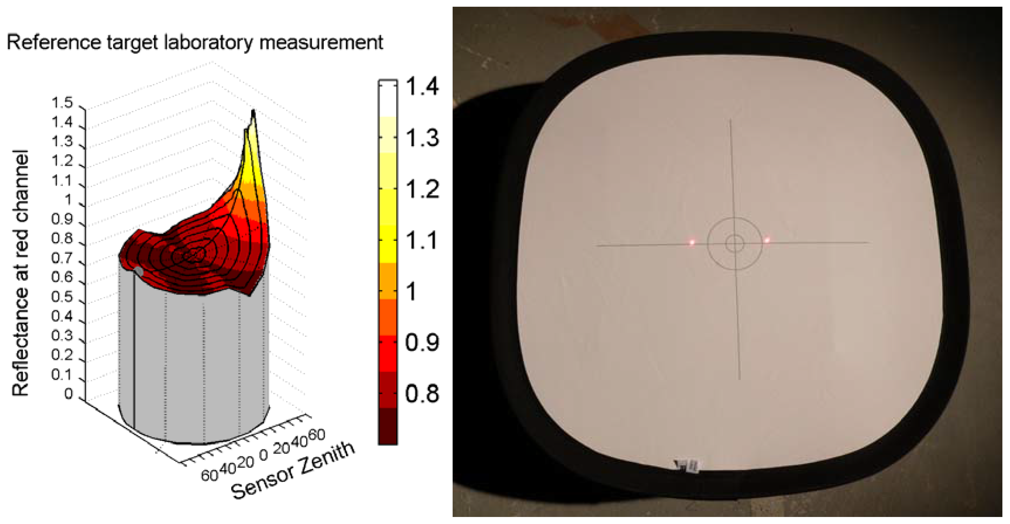
After the flat-field correction, the pixel intensity values were comparable to each other within one image. The reflectance factor of the target surface was calculated using the reference target method, which has also been used to correct large-scale aerial images [8,9]. A reference target (Figure 4) with known BRF had to be visible in each image, since the stability of the consumer camera was insufficient and the overall intensity level of the recorded pixel values varied between images. Also variations in the illumination conditions between the image acquisitions are corrected by the reference target. The reference target was manually picked from the images, the pixel intensity values of the target were recorded, and the view direction was retrieved from the UAV flight data. Pixels of the reference target were collected from an area of at least 10 pixels in diameter for adequate averaging.

Figure 4. Left: High specular reflectance can be observed in the reference target laboratory measurement BRF. Right: A picture of the reference target during the laboratory measurement. The two red laser dots indicate the measurement location.

Figure 4. Left: High specular reflectance can be observed in the reference target laboratory measurement BRF. Right: A picture of the reference target during the laboratory measurement. The two red laser dots indicate the measurement location.

The reference target was measured in the laboratory using the setup described in Section 2.2. The reflectance factor values of the reference target were retrieved from the laboratory measurement data for the same view and illumination geometry as in the UAV data. Laboratory measurement values were then used to normalize the reference target pixel intensity values retrieved from the image. These reference values were then used to normalize the entire image to create a reflectance factor image.

$$R_{ij}({\theta }_{sun},{\varphi }_{sun};{\theta }_{ij},{\varphi }_{ij})=R_{ref}({\theta }_{sun},{\varphi }_{sun};{\theta }_{ref},{\varphi }_{ref})\frac{D_{ij}({\theta }_{sun},{\varphi }_{sun};{\theta }_{ij},{\varphi }_{ij})}{D_{ref}({\theta }_{sun},{\varphi }_{sun};{\theta }_{ref},{\varphi }_{ref})}$$

(2)

The reflectance factor of a single pixel R_ji depends on the incident illumination direction and the observation direction. D_ij is the flat-field corrected pixel intensity value of the land surface from a single image. D_ref is the flat-field corrected mean pixel intensity value of the reference target in the same image, and R_ref is the laboratory-measured reflectance factor of the reference target.

3.4. Image Registration

A method was needed to orient the images so that the same area of land surface could be extracted from each image. Since no geometric correction was used, the images were distorted, and a simple three-point affine transformation did not yield accurate results, even though the sample surface was flat. Instead a transformation by Bookstein [10] was used. His method consists of a global affine part and a local part adding some warping to the transformation. This method has previously been used for image-to-map registration [11] and registration of digital images [12]. Piotr Dollar has implemented this method to a function in his Image and Video Toolbox for Matlab, which was used in this work.

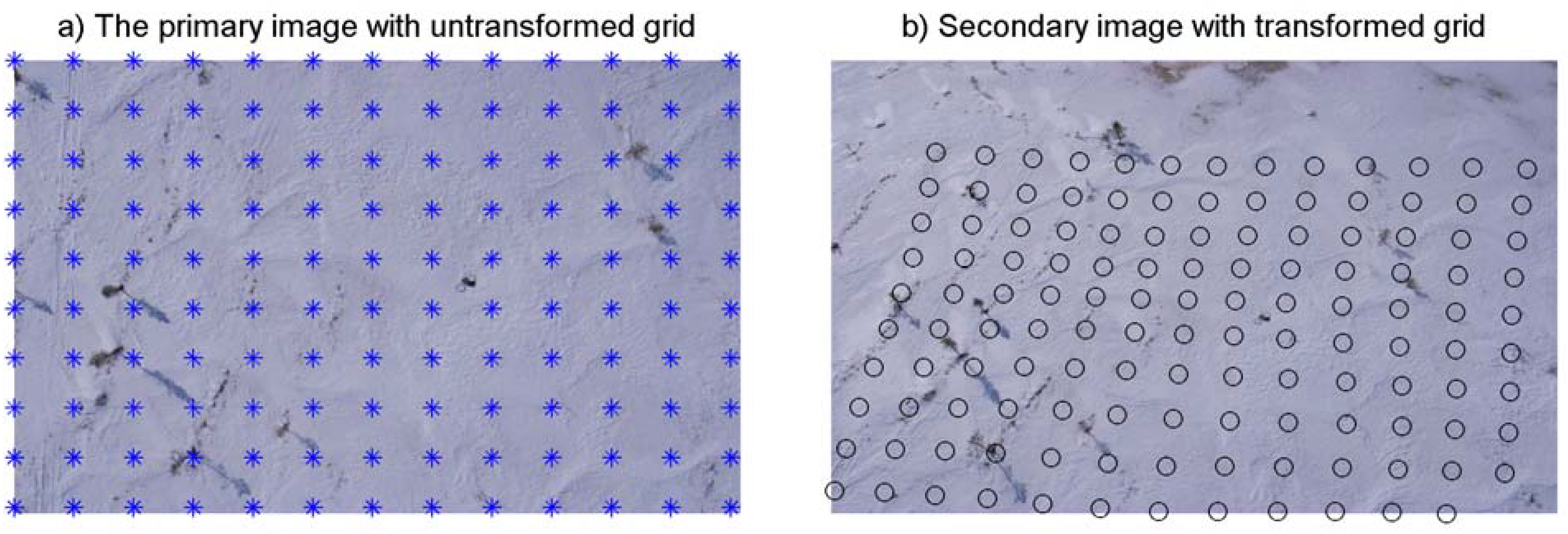
Approximately 20 ground control points were manually selected from each image, and the transformation was calculated using these points. One image was selected as a primary image, and all other images in the dataset were transformed to correspond with this image. The primary image was divided into equal-sized squares that determined the resolution of the bidirectional reflectance factor dataset in subsequent processing steps. To avoid unnecessary interpolation of pixel intensity values the images were not resampled; instead the grid in the primary image was transformed to correspond with each image (Figure 5).

Figure 5. Two images from the dataset with the grid-square corner points overlaid on top. (a) The primary image with the untransformed grid of 300 × 300 pixel squares. (b) Another image from the dataset with the transformed grid from the primary image.

Figure 5. Two images from the dataset with the grid-square corner points overlaid on top. (a) The primary image with the untransformed grid of 300 × 300 pixel squares. (b) Another image from the dataset with the transformed grid from the primary image.

The transformed squares were identified from each image, if inside the image bounds and the mean of the reflectance values for each camera channel were calculated within the squares. The position on the image plane was also recorded, and when combined with the flight data, the sensor direction relative to the illumination direction could now be calculated. This data was then combined to form the BRF of each square and recorded to an indexed database. The spatial resolution of the database depends on the size of grid squares used. A grid of 50 × 50 pixels is used, which means spatial resolution of about 50 cm. In Figure 5, a grid of 300 × 300 pixels is shown for clarity.

3.5. Modeling of the BRF

The BRF database can be used, for example, for modeling the surface BRF. A model describes the BRF of the surface with a number of parameters. For this data a simple three-parameter Rahman Pinty Verstraete (RPV) model [13] is fitted for visualization purposes.

$$Rs({\theta }_1,{\varphi }_1;{\theta }_2,{\varphi }_2)={\rho }_0\frac{{\cos }^{k-1}{\theta }_1{\cos }^{k-1}{\theta }_2}{{\left(\cos {\theta }_1+\cos {\theta }_2\right)}^{1-k}}F(g)\left[1+R(G)\right]$$

(3)

$$F\left(g\right)=\frac{1-{\Theta }^2}{{\left[1+{\Theta }^2-2\Theta \cos \left(\pi -g\right)\right]}^{1.5}}$$

(4)

$$\cos g=\cos {\theta }_1\cos {\theta }_2+\sin {\theta }_1\sin {\theta }_2\cos \left({\varphi }_1-{\varphi }_2\right)$$

(5)

$$1+R\left(G\right)=1+\frac{1-{\rho }_0}{1+G}$$

(6)

$$G={\left[{\tan }^2{\theta }_1+{\tan }^2{\theta }_2-2\tan {\theta }_1\tan {\theta }_2\cos \left({\varphi }_1-{\varphi }_2\right)\right]}^{1/2}$$

(7)

where reflectance factor R_s is a function of incident illumination directions θ₁ and ϕ₁, and observation directions θ₂ and ϕ₂. ρ₀ is a model parameter characterizing the reflectance intensity, k is a parameter indicating the level of anisotropy of surface reflectance, and Θ is a parameter describing the relative amount of backward/forward scattering.

4. Measurement Results

Two of the spring 2009 measurements using the UAV setup are described here. One measurement was taken to compare the UAV reflectance factor data to reference measurement data acquired simultaneously with a spectroradiometer. Another measurement was taken to determine the BRF of snow cover.

A measurement was taken on May 18, 2009 for concrete tiles, gravel targets and tarps (Figure 6).

The ASD FieldSpec Pro FR spectroradiometer was used to measure the nadir reflectance factor of each target about 30 minutes before the UAV was flown over. The purpose of this experiment was to validate the accuracy of the reflectance factor measured with the UAV, therefore only nadir images were captured at low altitude of 10–15 meters. Spatial resolution of around 4 mm was achieved, allowing large number of pixels to be averaged of each target. 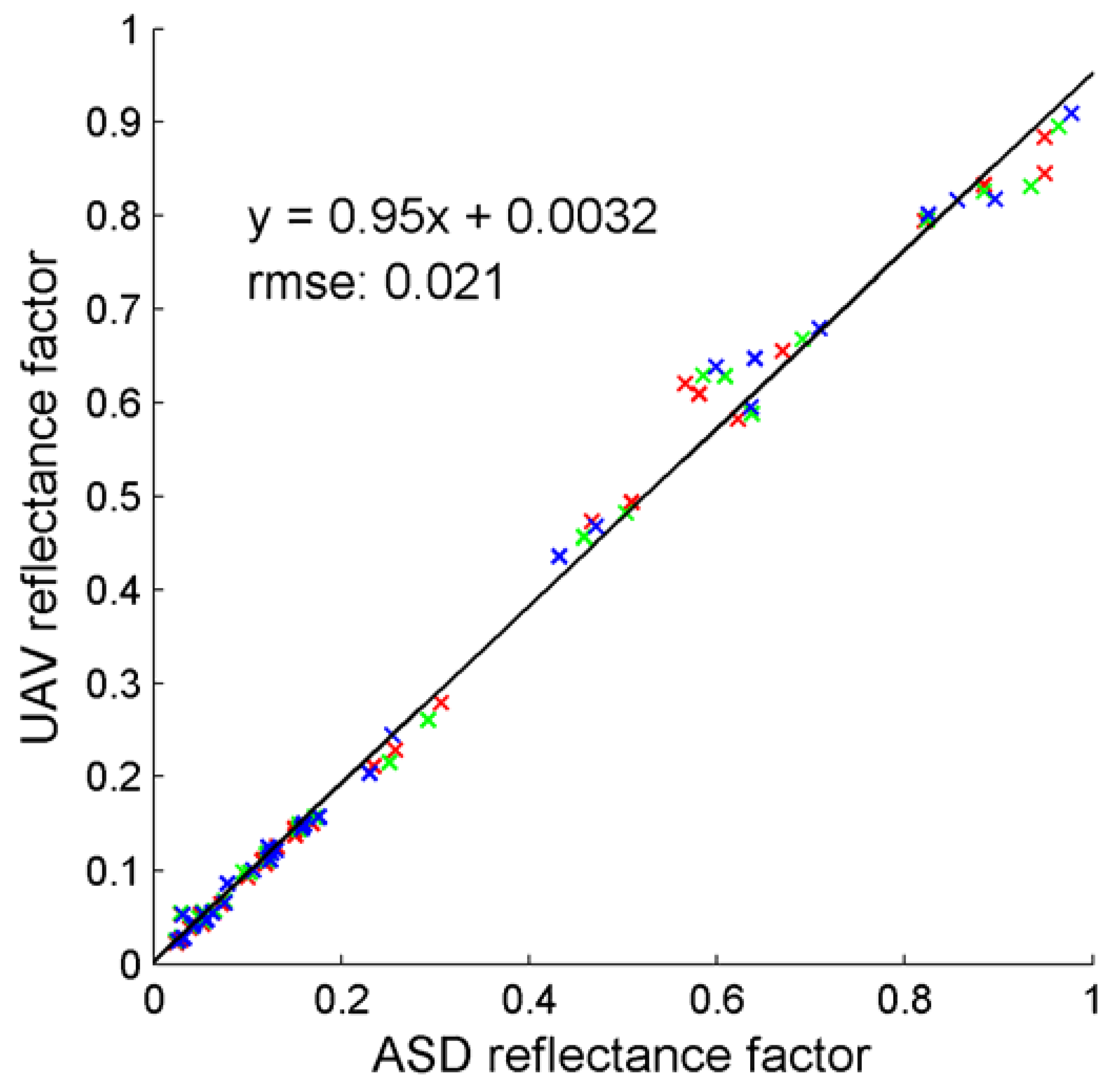Targets were manually selected from the image, and the reflectance factors were calculated by dividing averaged pixel intensity values of the targets by averaged pixel intensity value of spectralon (target 27 in Figure 6). The validation measurement data shows clear linearity between the ASD and UAV results (Figure 7).

Figure 6. Targets used for reflectance factor validation measurement. Targets 1–2 are light gravel brick painted with gray and white paint, 3–17 are concrete tiles painted with various paints or left unpainted, 18–23 are gravel samples from the Sjökulla test field, 24–27 are reference targets, 28–31 are plastic tarps painted with various black or white paints, and 32–34 are pieces of commonly available carpets.

Figure 6. Targets used for reflectance factor validation measurement. Targets 1–2 are light gravel brick painted with gray and white paint, 3–17 are concrete tiles painted with various paints or left unpainted, 18–23 are gravel samples from the Sjökulla test field, 24–27 are reference targets, 28–31 are plastic tarps painted with various black or white paints, and 32–34 are pieces of commonly available carpets.

Figure 7. A scatter plot of the validation measurement data. X axis: Ground reflectance factor data measured with ASD Field SpecPro from estimated red, green and blue channels. Y axis: Reflectance factor values extracted from the UAV image from the same targets and color channel as the ASD data. Red, green and blue crosses refer to the respective channel. A line is fitted to the data, and a clear linear relationship can be seen. Color targets 3, 5, 6, 7, 9, 17, and 22 (in Figure 6) were not used due to the unknown camera spectral response.

Figure 7. A scatter plot of the validation measurement data. X axis: Ground reflectance factor data measured with ASD Field SpecPro from estimated red, green and blue channels. Y axis: Reflectance factor values extracted from the UAV image from the same targets and color channel as the ASD data. Red, green and blue crosses refer to the respective channel. A line is fitted to the data, and a clear linear relationship can be seen. Color targets 3, 5, 6, 7, 9, 17, and 22 (in Figure 6) were not used due to the unknown camera spectral response.

Due to unknown spectral response of the camera RGB filter, the red, green and blue color bands used for ASD spectra are estimated from spectral response curves of a similar camera with known response. This makes it impossible to use the color targets for validation measurement since the ASD and camera responses cannot be accurately matched. For the grayscale targets, the root mean square error (RMSE) for a line fitted to the data is 0.021. This deviation from linear fit of about 0.02 in the measured reflectance factors increases confidence to the measurement results.

The BRF-measurement dataset described here was measured on April 22, 2009 during the Snortex snow-measurement campaign at Sodankylä, Finland. This dataset was measured during a calm and sunny day over a target area with various types of snow. The target area was situated on a flat, frozen swamp, with very few small trees. Concurrent reference measurement, taken with FIGIFIGO, took place just outside the bounds of the target area to avoid disturbing the UAV measurement. The reference measurement was used to validate the UAV data. Similar datasets of FIGIFIGO snow measurements from the 2008 campaign are presented in detail in article [14].

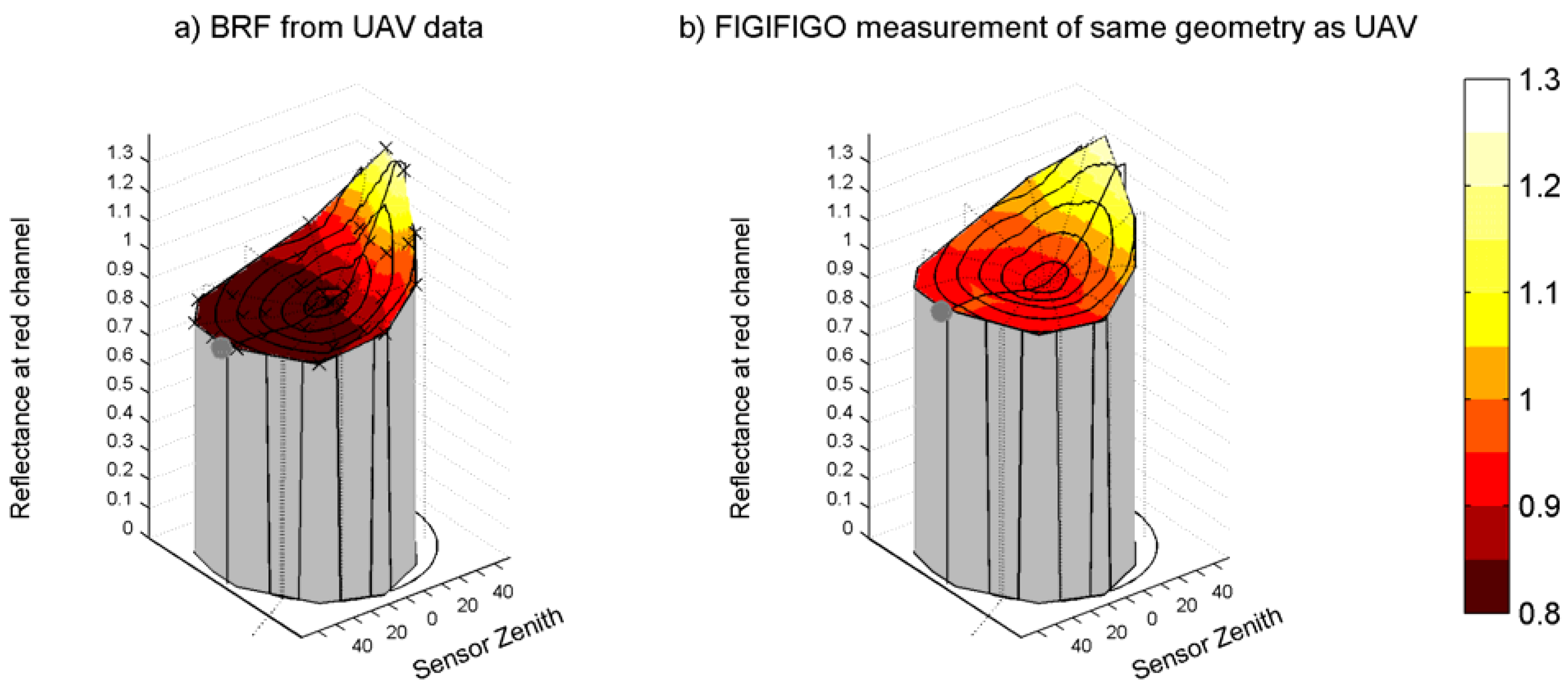
The UAV was programmed to take pictures of the target area from various directions, varying from the nadir direction to 50° from nadir. The images were processed as described in Section 3. Figure 8 shows a single measurement point from the UAV dataset and the FIGIFIGO reference data, which is interpolated to the same measurement geometry as the UAV data. Even though the sample is not the same for both measurements, similar characteristics can be detected. The BRF of snow cover has large spatial variance, which alone is enough to explain the observed difference.

Figure 8. (a) Reflectance factor plot of an area of smooth snow measured with UAV. (b) A similar, but not the same, sample of smooth snow measured using FIGIFIGO and interpolated to the same measurement geometry as the UAV data. Similar characteristics can be seen in both samples, although the overall intensity of the UAV sample is lower and specular reflection is higher.

Figure 8. (a) Reflectance factor plot of an area of smooth snow measured with UAV. (b) A similar, but not the same, sample of smooth snow measured using FIGIFIGO and interpolated to the same measurement geometry as the UAV data. Similar characteristics can be seen in both samples, although the overall intensity of the UAV sample is lower and specular reflection is higher.

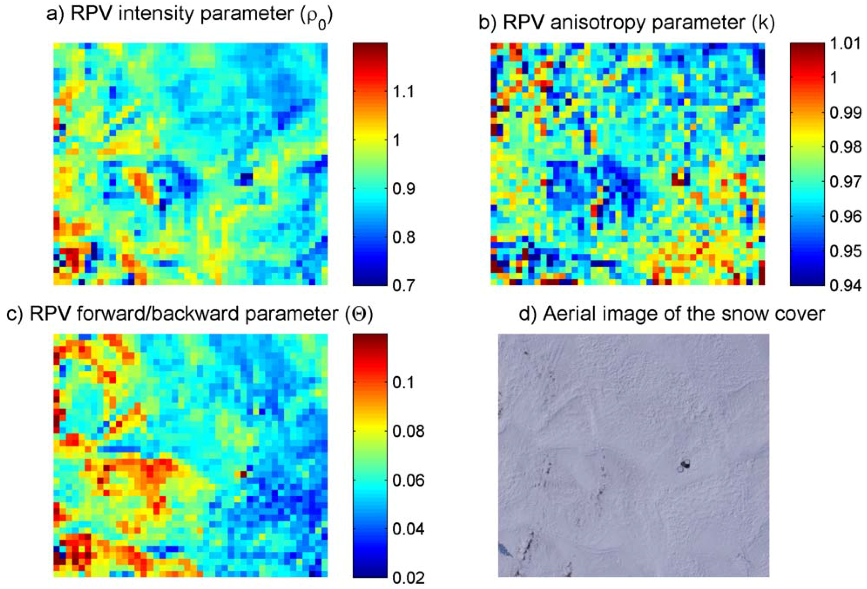
Figure 9 shows the data after the model fitting. A 50 × 50 pixel grid was used to sample the primary image to squares of approximately 0.5 × 0.5 m² spatial resolution. The RPV model was fitted to BRF data of each grid element and the model parameters were assembled to parameter maps. The parameter ρ₀ describing the overall intensity of the surface seems to correlate to the actual aerial-image surface brightness; darker spots on snow cover have a smaller intensity parameter value than the bright areas. The anisotropy parameter k has a higher value in rough parts of the snow cover, and the smooth surfaces have a higher forward/backward parameter Θ.

Figure 9. The Rahman Pinty Verstraete model parameter maps for the target area. The BRF data has been calculated from the images in a 50 × 50 pixel grid. Although the RPV model is not perfectly suited to model subtle variations in the snow cover, for example variations in the roughness of the snow cover can be observed by visually comparing the primary image and the parameter maps.

Figure 9. The Rahman Pinty Verstraete model parameter maps for the target area. The BRF data has been calculated from the images in a 50 × 50 pixel grid. Although the RPV model is not perfectly suited to model subtle variations in the snow cover, for example variations in the roughness of the snow cover can be observed by visually comparing the primary image and the parameter maps.

5. Discussion

The BRF data can be used for physical parameter extraction. For example, surface albedo [15], which is an important parameter for climate modeling. Henderson-Sellers suggests that error of ±0.01 in surface albedo can cause error of up to ±1 K to modeled global temperature [16]. The study further suggests that albedo accuracy of ±0.02 to ±0.05 is needed for climate modeling. From the BRF dataset described in this article, albedo can be calculated with very high spatial resolution, giving detailed information of the surface properties. Other studies [17,18] state that RMSE of Landsat satellite imagery is 0.02. When compared to this, the 0.021 RMSE of reflectance factor of our UAV system seems satisfactory.

The measurements described in this article were preliminary and thus some sources of error were omitted. (1) The diffuse light from the surroundings of the measurement site and sky has not been taken into account. The laboratory measurement of the reference target was lacking the diffuse component, which added some uncertainty to the calculated BRF. Additionally, at low altitudes, complicated atmospheric corrections are not needed, but recovering the clean BRF would require some corrections to take diffuse light into account. (2) Some change in illumination angle occurred affecting the shape of the measured BRF, although duration of the BRF measurement was short (~10 min). The reference target only corrected for the changes in level of illumination, not the changes in BRF. (3) During the reflectance factor accuracy measurement the illumination angle changed about 3° between the ASD and UAV measurements. Also the view direction was approximated to nadir for all targets, as in reality it varied because the targets were in the same image.

A measurement is needed to verify the spectral response of the digital camera. This would provide reflectance factors that are more detailed and accurately comparable to other instruments. The camera also has some uncertainty with the shutter, causing some images to be slightly brighter than others. Also, the optics have large geometric distortions. Thus, better camera options should be explored.

Spectralon panel is generally a good reference target, but large enough spectralon panels are not available for reasonable price. Therefore a larger, but less ideal, reference was used instead, requiring BRF normalization. The reference target used was not Lambertian enough, and especially at low illumination angles it had high specular reflection. The laboratory measurement did not describe the reference target’s BRF precisely, as a model fitted to the data was not of high enough order to accurately model the large specular spike. This in turn caused overestimation of the specular characteristics of the actual target BRF. For future measurements better reference targets, such as those used for large-format digital photogrammetric sensors [19], are needed. However, even with these limitations, the quality of the data is reasonably good.

6. Conclusions

A method for mapping the bidirectional reflectance factor (BRF) of ground surface, using a micro unmanned aerial vehicle and consumer camera, is described. The acquired images are corrected for vignetting, calibrated with a reference target and registered using a corresponding point method. A BRF dataset is created from the reflectance values.

It was found that autonomous unmanned aerial vehicles can be used in waypoint navigation mode to fly predefined paths over the target with a high level of accuracy, taking observations in well-defined locations from selected directions. This allows the complex measurement geometry required for surface BRF measurements. The system was easy to program and it was also found to be reliable. All operations were possible to perform easily and conveniently by two people in the field.

It was shown that, inherently unstable consumer-level cameras can be configured to produce useful results. For successful calibration, a reference target had to be visible in all images, and its anisotropy and reflectance properties had to be known to a high accuracy. Furthermore, the use of reference automatically corrected for illumination variations caused by atmosphere.

We discovered that the UAV setup can produce reflectance factors that are close to those measured with a spectroradiometer. Reflectance factors taken with the camera have internal accuracy of about 0.02 RMSE, and the reflectance factor behaves linearly with increasing target brightness. Thus, accurate and applicable BRFs of land-surface targets can be measured using a micro UAV and a consumer camera.

The BRF retrieval method can be used for various applications. The method provides data for retrieval of surface albedo and for automated land cover classification. The data can also be used for upscaling the on-ground BRF measurements to larger areas, providing a tool for the evaluation of satellite and airborne data. The flexibility of an automated UAV allows more freedom and fills the gap between on-ground and airborne sensing.