Reconstructing High-Resolution Coastal Water Quality Data Based on a Deep Learning Multivariate Downscaling Approach

Highlights

What are the main findings?

• Incorporating spatial modes as training inputs enhances downscaling performance compared to direct time- series learning by effectively capturing intrinsic spatial features.
• The downscaled fields exhibit fine-scale gradients and continuous structures invisible in original satellite observation.

What is the implication of the main finding?

• Pre-trained time-invariant spatial modes can be used to reconstruct statistically consistent, high-resolution ocean fields directly from low-resolution satellite observation during any independent testing.
• By effectively capturing intrinsic spatial features, the proposed approach generates meaningful sub-grid information, thereby overcoming the resolution constraints in standard coastal remote sensing data and enhancing its applicability.

Abstract

The availability of high-resolution oceanographic data is critical for evidence-based coastal environmental management and climate resilience planning, yet it remains constrained by observational gaps and the prohibitive computational cost of fine-scale hydrodynamic modeling. While downscaling techniques provide a viable pathway, current data-driven approaches often lack statistical physical associations, overlook multivariate environmental interactions, and struggle to represent complex coastal topography. To address these limitations, we present MEOFGAN—an environmentally informed downscaling framework that integrates multivariate empirical orthogonal function (MEOF) decomposition with a generative adversarial network (GAN). The model extracts physically interpretable spatial modes of coupled ocean variables, learns their cross-scale transitions through adversarial training, and systematically incorporates high-resolution bathymetry as a static environmental constraint to enhance spatial fidelity. When applied to the Bohai Sea, MEOFGAN successfully downscales sea surface temperature (SST) and sea surface height (SSH) from 1/4° to 1/12°, achieving error reductions of 30–68% compared to benchmark methods while preserving ecologically relevant structural patterns (SSIM > 0.92). The framework demonstrates strong generalization by reconstructing 500 m resolution distributions of chlorophyll-a (Chl-a), dissolved oxygen (DO), and salinity in Bohai Bay, capturing fine-scale environmental gradients during a documented algal bloom event. This work establishes a methodological framework that can be transferred as a paradigm for generating high-resolution coastal datasets. Rather than serving as a universally transferable pre-trained model, the framework requires region-specific training and application. Data generated in this manner can directly support water quality monitoring, eutrophication assessment, habitat mapping, and regionally tailored climate adaptation strategies.

1. Introduction

The coastal zone is a dynamic region at the interface between the land and the ocean where the tides, the ebb and flow of sediments, and pollution take place. All of these actions occur at a finer spatial scale. The processes are essential for coastal zone management, flood risk assessment, storm surge forecasting, and understanding the impacts of climate change on vulnerable coastlines [1,2]. Therefore, acquiring high-resolution data in these regions is essential for accurate simulation, prediction, and informed decision-making.

However, obtaining such high-resolution data is subject to multiple constraints. Although standard in situ measurements provide valuable information, they are often sparse and expensive to maintain and, thus, unable to provide full synoptic coverage [3]. Satellite remote sensing has extensive spatial coverage but is inherently limited by revisit frequency, spatial resolution, and sensitivity to atmospheric interference like cloud cover [4]. Moreover, different ocean variables, such as temperature, salinity and chlorophyll-a (Chl-a), exhibit distinct physical properties which affect the achievable resolution across datasets. High-resolution numerical modeling presents a theoretical solution. However, its computational cost and resource demands become exorbitant when attempting to resolve fine-scale features, especially in coastal areas with complex bathymetry and topography. Given the above considerations, downscaling methods have emerged as an effective technical way for efficiently generating high-resolution ocean data through the integration of coarse data [5,6].

Current methods of downscaling can be generally categorized into dynamical downscaling, statistical downscaling (SD), and the combined methods [7]. Dynamical downscaling takes advantage of physical mechanisms and utilizes numerical models at high resolution that are usually driven by large-scale low-resolution data as boundary conditions [8,9,10]. Giorgi [11] demonstrated that nesting high-resolution regional climate models can better simulate regional climate features. Jacob and Stanev [12] were able to achieve hydrodynamic simulations at 50 m resolution in coastal areas using 7 km boundary conditions. By establishing a correspondence with the relevant physical laws, this procedure can identify the dynamical mechanisms responsible for observed phenomena. However, it is computationally expensive and sensitive to uncertainties in boundary conditions. For instance, high-resolution regional ocean modeling often requires thousands to tens of thousands of CPU hours per simulation year depending on the model complexity and resolution [13,14]. In contrast, statistical downscaling establishes relationships to be computed from low- and high-resolution data and has the advantages of requiring less computational resources and being easier to apply [15,16]. Traditional techniques include bilinear interpolation, multiple linear regression [17], and quantile perturbation methods [18]. However, these methods depend highly on long-term high-quality observational data to build suitable statistical models [19], which consequently limits their performance in data-scarce regions.

As artificial intelligence (AI) methods have been developed in recent years, deep learning (DL) methods have been applied to downscaling for many scientific and engineering purposes due to their ability to perform nonlinear mapping and represent features [20,21]. Super-resolution (SR) technology is well known in terms of image process. Notable approaches include the convolutional neural network-based SRCNN [22], the residual learning-based EDSR [23], and the meta-learning-integrated zero-shot super-resolution model MZSR [24], which were used to reconstruct high-resolution details from low-resolution images. These methods differ from the aforementioned SD methods. The SD methods establish nonlinear mapping relationships between geophysical fields at various scales, while the SR methods focus on recovering image degradation resulting from information propagation processes. DL-based downscaling methods have been widely applied in reconstructing sea surface temperature (SST) [25,26,27,28,29], sea surface height (SSH) [30,31], and ocean wave fields [32,33,34]. These studies showed that DL can easily extract multi-scale oceanic characteristics. For instance, Thiria et al. [35] developed a multi-scale convolutional neural network that improved SSH and surface current fields in the North Atlantic from 1° to 1/8°, resolving the fine structures of mesoscale eddies. Zhang et al. [36] employed a generative adversarial network (GAN) to accomplish global SSH reconstruction at 1/12° resolution; this network estimates ocean kinetic energy spectra much more accurately. However, while some methods can perform in the open ocean in a satisfactory manner, they face great challenges when applied to coastal waters, where the environment is complex in its topography and often involves coupled dynamic processes across multiple scales [37]. The direct development of computer vision-based SR models has several limitations: First, they lack interpretability and agreement with physical mechanisms. Most downscaling models based on DL behave like typical “black boxes” for which the mapping of low to high resolution lacks physical interpretation [38]. Such approaches primarily learn statistical patterns in data rather than actual underlying physical mechanisms. In addition, cooperative reconstruction for multiple variables remains insufficient. Ocean parameters—such as SST, SSH, and SSS—are tightly coupled through physical relationships. Most existing downscaling approaches, nonetheless, reconstruct a single variable independently. This results in inadequate physical consistency of the reconstructed fields. The generated SSH and surface current fields, for instance, may not satisfy geostrophic balance, limiting their utility in data assimilation and ocean forecasting [39]. Additionally, they are unsuitable for complex coastal topography. Coastal regions are significantly influenced by bathymetry, coastline irregularity, and shallow-water effects, none of which are addressed in standard SR models. Studies revealed that in regions with steep slopes, straits, and islands, SR models that do not take topography into account tend to produce large errors in the reconstruction of dynamic features [40]. They are especially inadequate for the representation of essential processes such as vortex shedding, upwellings, and topography-induced tidal mixing.

To meet the increasing demand for high-resolution reconstruction in coastal waters and to address existing data-driven schemes’ limitations, this study proposes a new hybrid downscaling scheme—MEOFGAN (multivariate empirical orthogonal function-based generative adversarial network)—that integrates the existing data from multiple sources to reconstruct high-resolution oceanic fields. The scheme establishes a methodological framework that balances accuracy and physical plausibility by leveraging the joint characteristics of multivariate ocean variables along with topographic information. Importantly, this framework is not designed as a universally transferable pre-trained model; instead, it requires region-specific training and application, thereby defining its scope as a transferable paradigm rather than a directly deployable model. The MEOFGAN architecture is constructed with two coordinated modules. First, the spatial structures are characterized through the dominant spatial modes (EOFs) extracted from MEOF. The second module designs a GAN architecture to learn the spatial mapping from low to high resolution, incorporating bathymetric data as additional static information during training to enhance spatial structure learning. To evaluate the effectiveness of the proposed method, the Bohai Sea and Bohai Bay are selected as the study areas due to their semi-enclosed nature and complex coastlines. Given the well-established correlation between SST and SSH and their compatibility with the MEOF framework [41,42], downscaling experiments for these two variables are first conducted in the Bohai Sea. Beyond statistical correlation, their physical coupling provides a process-based rationale: SST influences SSH via thermal expansion, while SSH-gradient-driven geostrophic currents regulate horizontal heat transport. Joint downscaling thus preserves this thermodynamic–dynamic consistency.

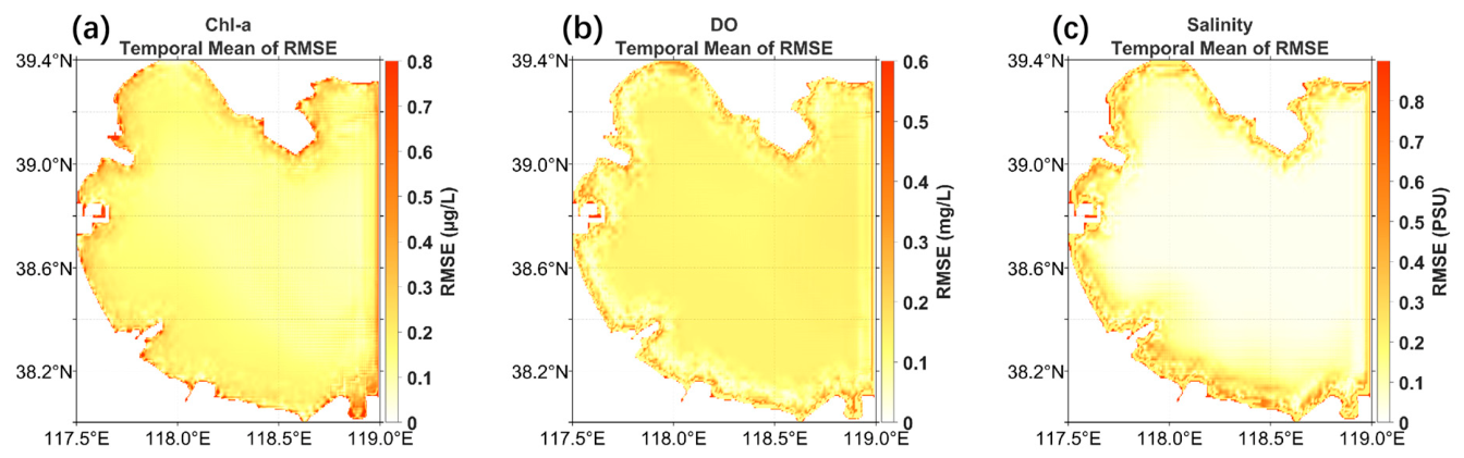
Furthermore, Chl-a, DO, and salinity are key indicators of coastal ecosystem health [43], and their physical–biogeochemical couplings justify joint downscaling. Chl-a, representing phytoplankton biomass, directly modulates DO dynamics through photosynthetic oxygen production and oxidative decomposition. Salinity affects density stratification and water mass distribution, thereby controlling vertical exchange efficiency, benthic nutrient regeneration, and upward nutrient supply—indirectly regulating phytoplankton biomass and associated oxygen consumption. To this end, these three variables are integrated into a unified downscaling framework to preserve the coupled vertical-exchange–productivity–oxygen consumption process. Accordingly, a downscaling experiment for Chl-a, DO, and salinity is conducted in Bohai Bay to evaluate the proposed method in terms of spatial detail fidelity and temporal stability.

The remainder of this paper is organized as follows: Section 2 describes the study area and datasets, Section 3 details the proposed methodology and experimental setups, Section 4 presents results and discussion, and Section 5 concludes the whole study.

2. Study Area and Data

2.1. Study Area

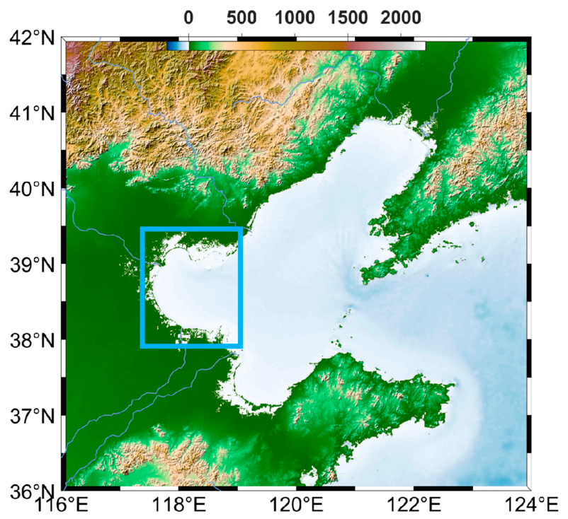
This study focuses on the Bohai Sea, China—a semi-enclosed basin located in 36°–42°N and 116°–124°E, as shown in Figure 1. Located in the warm temperate East Asian monsoon zone, the average depth here is 18 m. The region experiences four distinct seasons, and the marine environmental conditions display strong seasonal variability. The SST can drop to about 1 °C in winter and exceeds 20 °C in summer. These thermal conditions lead to a strong seasonal thermocline, and strong spatiotemporal variability in different marine elements, such as SST and SSH, occurs. Taking into account the complicated interactions among physical, biochemical processes, and large concentrations of people in the surrounding area, the Bohai Sea is selected as the regional area for conducting multivariate downscaling studies based on available data.

In order to test whether the proposed downscaling scheme can be transferred to regions with higher data resolution requirements, we incorporated high-resolution model data alongside remote sensing data; the experiments were carried out in the local area of Bohai Bay. The Bohai Bay (38°–39.4°N, 117.5°–119°E), as shown in the blue box in Figure 1, is a coastal area strongly influenced by human activities, riverine discharge, and climate change. Given the spatial variation in these interactions, a comprehensive, high-resolution dataset for the Bohai Bay is thus fundamental to quantify its fine-scale processes.

2.2. Data: CMEMS Ocean Reanalysis Data

The SST, SSH, and SSS data were sourced from ocean reanalysis products at two spatial resolutions. High-resolution data (1/12°) were obtained from the global ocean physical reanalysis product (GLORYS12V1) provided by the Copernicus Marine and Environment Monitoring Service (CMEMS). Low-resolution data (1/4°) were extracted from the CMEMS global ocean ensemble physical reanalysis product. The latter quantifies uncertainties in ocean state estimation through a multi-member ensemble approach and assimilates multi-source observations, including multi-generation satellite altimeters, providing physically consistent large-scale dynamical field information. The dataset provides continuous coverage from January 1993 onward; the period of 1993–2020 was selected for this study.

DO data were obtained from the global ocean biogeochemical hindcast dataset released by CMEMS. This dataset is based on a coupled physical–biogeochemical model forced by historical atmospheric fields, aiming to reproduce long-term variations and climatic characteristics of biogeochemical variables, thereby providing physically consistent simulation fields for mechanistic studies. Its original spatial resolution is 1/4°.

2.3. Data: Satellite Remote Sensing Data

Satellite-derived chlorophyll-a concentration data was sourced from the “Global Ocean Colour Biogeochemistry L4” product released by CMEMS. This product generates spatially complete daily chlorophyll-a concentration fields by merging ocean-color observations from multiple satellites and applying an optimal interpolation algorithm, with an original spatial resolution of about 4 km. To integrate these data into a unified analytical framework and facilitate comparative validation with reanalysis and simulation data, the satellite product was also regridded and resampled to the standard 1/12° grid. This processing preserves the advantage of satellite data in capturing spatial heterogeneity of algal biomass in nearshore and bay areas while ensuring consistent spatial referencing across all datasets. Resampled data from 1997 to 2020 were used to support the characterization and analysis of long-term ecological evolution in the Bohai Bay.

2.4. Data: Delft3D Simulation Data

To address the resolution limitations of existing satellite and reanalysis data in capturing fine-scale structures of nearshore eco-dynamic processes, this study employed the physically-driven Delft3D modeling framework to construct a high-resolution hydrodynamic–biochemical reference field for the Bohai Bay. The model utilizes a curvilinear grid system aligned with geographical coordinates at a spatial resolution of 500 m. The open boundaries of the model were forced with large-scale Bohai Sea reanalysis data. The water quality module was specifically parameterized according to the environmental characteristics of the Bohai Bay, which can simulate more than 23 variables such as the nutrients, Chl-a, DO, etc. Based on the above setup, high-resolution simulated outputs for the entire year of 2016 were obtained at an hourly interval, yielding 8784 valid samples per variable. To construct and objectively evaluate the downscaling model, we focus on three key surface variables: Chl-a, DO, and salinity. Their data from January to August were designated as the training set (5856 samples, 66.7%) for parameter construction and training. Data from September to December were reserved as an independent test set (2928 samples, 33.3%) to examine the model’s generalization capability and stability during validation periods. This dataset provides a reliable “quasi-truth” benchmark for evaluating the performance of downscaling methods at sub-kilometer scales.

2.5. Data: Static Bathymetric Data

There are many factors that influence oceanic elements, among which bathymetry is a significant one. It can be assumed that the variations in water elements at the same bathymetric location exhibit certain inherent regularities. Therefore, in the deep learning of downscaling, bathymetry can serve as a constraint to strengthen the corresponding relationships of ocean elements transitioning between different scales at grid points with similar bathymetry. Bathymetric data were obtained from the latest version of the General Bathymetric Chart of the Oceans (GEBCO). This dataset integrates multi-source measured data, including shipborne soundings and satellite-derived bathymetry, providing a high-resolution global elevation grid at 15-arc-second intervals (approximately 463 m). To match the numerical experiment setup, the original data were clipped to the study domain and resampled to grids identical to those of the high- and low-resolution ocean reanalysis datasets. This static bathymetric field served as a key bottom boundary condition and was input into the neural network as a static variable representing topographic constraints, helping the model better understand and maintain the physical relationship between ocean dynamic processes and seabed topography during downscaling.

3. Methods

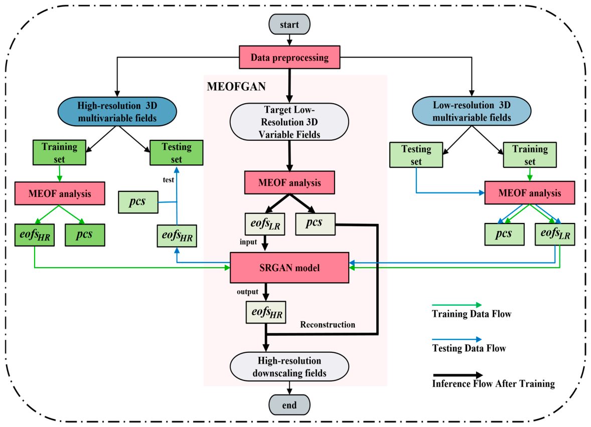
This study develops a hybrid deep learning downscaling scheme that integrates the strengths of MEOF decomposition and GAN methods to achieve accurate multivariate joint downscaling. As illustrated in the flowchart (Figure 2), prior to the main downscaling procedure of MEOFGAN, a key data preprocessing module is constructed in which seafloor topography data are regridded to the target resolution via interpolation (see Section 3.1). Subsequently, both high- and low-resolution datasets are divided into training and testing sets in the same proportion. They are then decomposed via MEOF to obtain multivariate joint evolution time series and spatial modes, which lays the foundation for the subsequent downscaling structure (see Section 3.2). Building upon this, an adversarial network model comprising a generator and a discriminator is constructed, trained on the training set, and validated on the testing set (see Section 3.3). The main downscaling framework of MEOFGAN adopts a modular architecture, integrating three core components—a prior model module, a mapping module, and a reconstruction module—forming a complete workflow (see Section 3.4). To validate the synergistic effects of different variables during downscaling training and the effectiveness of the proposed framework, a series of comparative experiments are designed. The experiments first verify the method in the Bohai Sea region with complete data coverage and then extend it to the more refined Bohai Bay area to examine the applicability of the method across different geographical scales (see Section 3.5).

3.1. Data Preprocessing

As detailed in Section 2, bathymetric data is one of the factors influencing marine elements, and its observation possesses high resolution compared to sea surface variables. To effectively assimilate seafloor topography into our model, we implemented essential preprocessing procedures on the bathymetric dataset. The preprocessing workflow initially involved extracting pure marine topography by eliminating terrestrial data, which substantially reduced computational load and improved processing efficiency. Subsequently, the marine bathymetry was resampled to target resolutions of 1/12° and 1/4° using nearest neighbor interpolation (NNI), ensuring spatial consistency with the downscaling framework. Crucially, unlike SST and SSHA, which vary daily, bathymetry is treated as a static, time-invariant field. For the purpose of matrix construction in the subsequent MEOF analysis, this static field is conceptually repeated across all time steps, serving as a constant spatial background constraint.

For other marine variables, we executed a rigorous data preprocessing protocol to guarantee analytical reliability. This protocol comprised two critical steps: (1) removal of climatological signals to isolate interannual variability patterns and (2) standardization to eliminate dimensional discrepancies among multivariate datasets. These procedures not only effectively suppressed seasonal biases and unit inconsistencies but also significantly enhanced the detection capability for oceanic anomalous signals. After preprocessing, the static bathymetry grid and the dynamic anomaly fields of SST/SSHA are spatially aligned and ready for joint matrix construction.

3.2. MEOF Analysis

EOF decomposition, initially introduced by Pearson and later adapted for meteorological applications by Lorenz, is a powerful statistical tool widely used in climate and oceanographic studies to analyze the spatial and temporal variability of geophysical fields [44]. The primary objective of EOF analysis is to decompose a variable field into a set of orthogonal spatial patterns, known as EOFs, and their corresponding temporal coefficients, referred to as principal components (PCs). This decomposition allows for the extraction of dominant modes of variability, which often represent underlying physical processes or phenomena.

The computational procedure of MEOF analysis is fundamentally similar to that of conventional EOF methods, with the core distinction lying in the construction approach of the initial matrix. Following the preprocessing described in Section 3.1, we construct a joint anomaly matrix by concatenating the normalized SST anomalies, normalized SSHA anomalies, and the static normalized bathymetry field as follows:

$$X_{N\times M}=\left[\begin{array}{ccccc}{X}_{\mathrm{1,1}}^{SST}& \cdots & X_{1,m}^{SST}& \cdots & X_{1,M}^{SST}\\ ⋮& \ddots & ⋮& \ddots & ⋮\\ X_{n,1}^{SST}& \cdots & X_{n,m}^{SST}& \cdots & X_{n,M}^{SST}\\ X_{\mathrm{1,1}}^{SSHA}& \cdots & X_{1,m}^{SSHA}& \cdots & X_{1,M}^{SSHA}\\ ⋮& ⋮& ⋮& \ddots & ⋮\\ X_{n,1}^{SSHA}& \cdots & X_{n,m}^{SSHA}& \cdots & X_{n,M}^{SSHA}\\ X_{\mathrm{1,1}}^{Bathy}& \cdots & X_{1,m}^{Bathy}& \cdots & X_{1,M}^{Bathy}\\ ⋮& \ddots & ⋮& \ddots & ⋮\\ X_{n,1}^{Bathy}& \cdots & X_{n,m}^{Bathy}& \cdots & X_{n,M}^{Bathy}\end{array}\right]$$

(1)

where $X_{n,m}^{SST}$, $X_{n,m}^{SSHA}$, and $X_{n,m}^{Bathy}$ are the normalized values of SST anomaly, SSHA, and bathymetry, respectively, at the $n^{th}$ spatial grid point on the $m^{th}$ day. The matrix dimensions are $N \times M$ (where $N = 3n$), with n representing the number of spatial points for each variable, $N$ representing the number of spatial points of all variables, and $M$ representing the temporal length.

Then, the covariance matrix $C_{N\times N}$ of matrix $X_{N\times M}$ can be calculated as:

$$C_{N\times N}={\displaystyle \frac{1}{M}}{X}_{N\times M}\times X_{N\times M}^T$$

(2)

The eigenvalues (${\lambda }_1, \dots , {\lambda }_N$) and eigenvectors $V_{N\times N}$ of $C_{N\times N}$ can be expressed as follows:

$$C_{N\times N}\times V_{N\times N}=V_{N\times N}\times {\Lambda }_{N\times N}$$

(3)

$${\Lambda }_{N\times N}=diag\left({\lambda }_1, {\lambda }_2,\dots ,{\lambda }_N\right)$$

(4)

where ${\lambda }_i\left(i=\mathrm{1,2},\dots ,N\right)$ are arranged in descending order. Each non-zero eigenvalue corresponds to a column of eigenvectors, also referred to as the spatial pattern. For example, the eigenvector corresponding to ${\lambda }_1$ is called the first spatial pattern (i.e., the first column of $V_{N\times N}$), and so on. The spatial patterns are projected onto the matrix $X_{N\times M}$ to obtain the PCs corresponding to the eigenvector:

$${PC}_{N\times M}=V_{N\times N}^T\times X_{N\times M}$$

(5)

Through MEOF analysis, both the high-resolution training dataset and validation dataset in the study area are decomposed into EOFs and their corresponding PCs. The data of each row in the ${PC}_{N\times M}$ corresponds to the PCs of each column of eigenvectors. The PC of the first spatial pattern corresponds to the first row of ${PC}_{N\times M}$, and so on. By selecting the spatial and temporal components that account for the first 99% of the variance, we can represent the primary modes of joint evolution of the variables, significantly reducing the data volume while retaining the essential information. For clarity, the spatial modes of the high-resolution data are abbreviated as ${eof}_{HR}$, while those of the low-resolution data are abbreviated as ${eof}_{LR}$. Further consideration is required regarding the analysis of these orthogonal spatial modes.

3.3. GAN Model

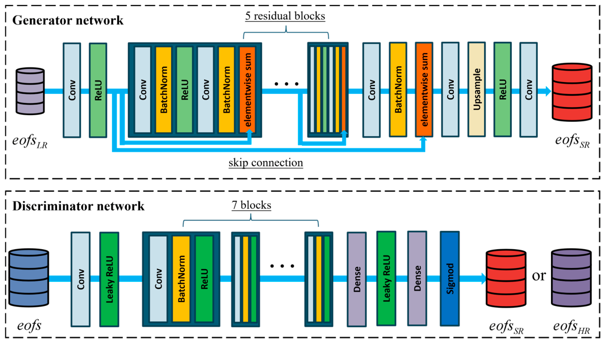
Upon completing the MEOF decomposition, we obtained spatial modes containing joint information from multiple oceanographic variables. To establish the mapping relationship between high- and low-resolution datasets, we developed a GAN architecture consisting of two core components: a generator and a discriminator (Figure 3).

The generator network takes low-resolution spatial modes as input and employs a deep residual architecture to maximally capture latent information within the input modalities. The input layer processes low-resolution fields using 3 × 3 convolutional kernels with LeakyReLU activation (α = 0.2), followed by a series of residual blocks. Each residual module incorporates two convolutional layers (Conv) with batch normalization (BatchNorm) and ReLU activation to enhance nonlinear feature extraction. A pivotal design element is the feature summation operation during high-resolution reconstruction, which not only strengthens information transfer efficiency between feature layers but also mitigates the risk of critical information being diluted through deep convolutional operations. The architecture progressively increases output feature map resolution through upsampling layers, ensuring the generated high-resolution outputs accurately preserve the detailed information inherent in the original high-resolution images.

The discriminator is designed to distinguish between real high-resolution images (HR) and generator-produced samples (SR). Its architecture utilizes convolutional layers and dense (Dense) layers, with LeakyReLU activation further enhancing sensitivity to subtle features. Multiple convolutional layers enable deep feature extraction from input data, while a final sigmoid activation function produces binary classification outputs to determine image authenticity. The discriminator also adheres to a hierarchical convolutional design philosophy, dynamically adjusting feature map resolution to enable more precise analysis of complex input characteristics.

3.4. MEOFGAN Framework Design

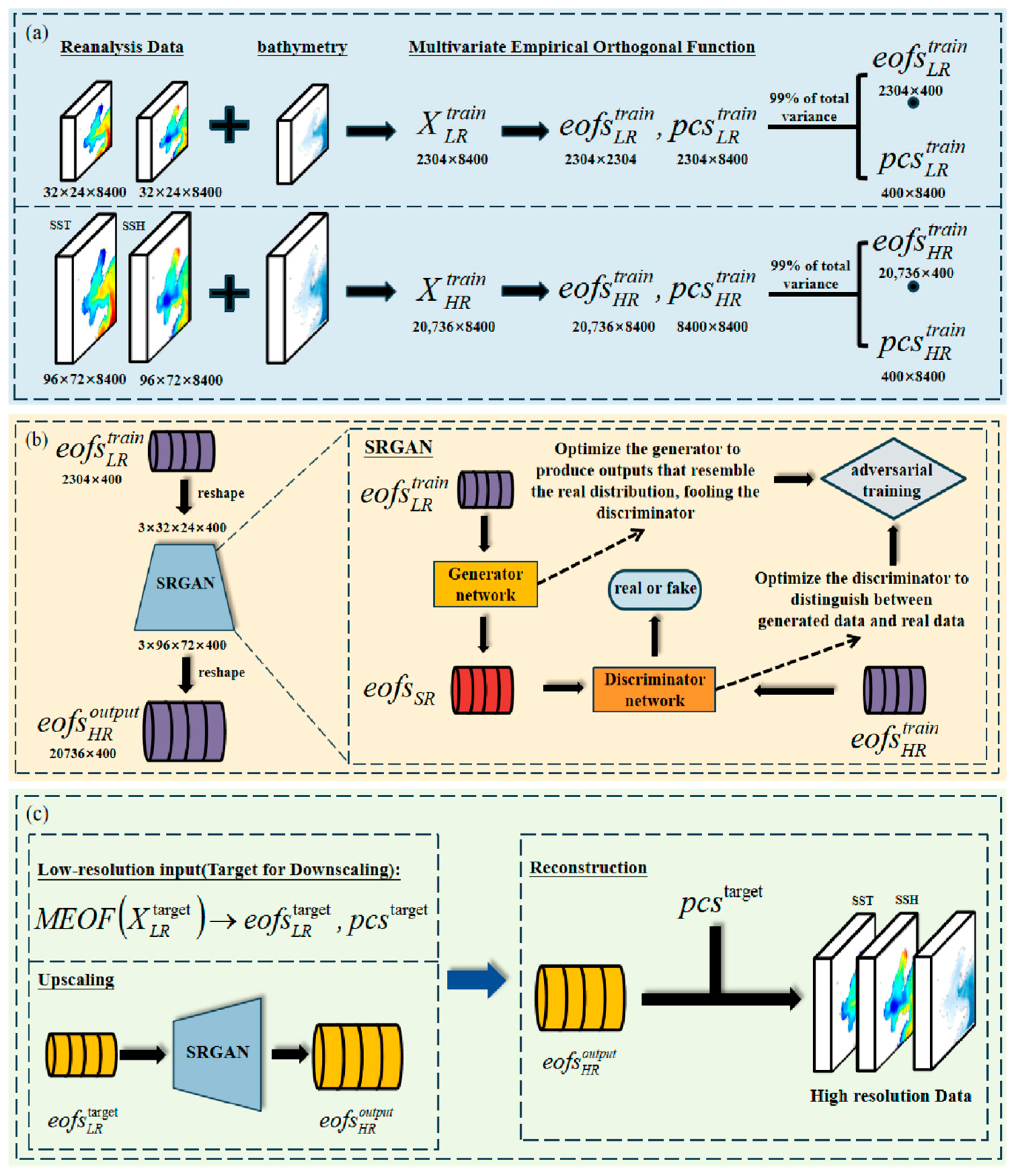
To effectively achieve multivariable downscaling, we propose a standardized workflow centered on an adversarial neural network. The framework adopts a modular design, integrating three core components: (a) data processing, (b) mapping, and (c) downscaling and reconstruction (Figure 4).

(1)

Data processing module: this module [Figure 4a] preprocesses and extracts feaatures from multiple types of marine reanalysis data and bathymetric data for downstream modules. The procedure is as follows. First, data from 1993 to 2015 are concatenated and reorganized. Then, based on native resolution, the data are divided into two groups and subjected to MEOF decomposition to extract joint evolution modes.

Although bathymetry is time-invariant, its inclusion in MEOF is mathematically valid, as MEOF operates on the joint spatial covariance matrix across variables rather than on temporal covariances alone. The static bathymetry vector contributes to off-diagonal blocks of this matrix through its spatial pattern, capturing how bathymetry spatially covaries with sea surface temperature (SST) and sea surface height anomaly (SSHA). Given the pronounced spatial heterogeneity of bathymetry, these cross-covariances are non-zero, allowing the joint modes to naturally encode bathymetry-conditioned SST–SSHA couplings.

Mechanistically, incorporating bathymetry enhances both the interpretability and reconstruction performance of MEOF. While SST–SSH combinations capture statistical covariations among surface variables, they lack spatial anchoring. Adding stationary bathymetry restructures the covariance matrix to also encode couplings between surface dynamics and seafloor topography. The resulting spatial modes link SST–SSHA covariability to specific topographic features. During the reconstruction phase, these spatial modes serve as spatially anchored templates, facilitating more accurate transformation of the dynamical information implicit in low-resolution fields into high-resolution structures with statistical physical associations at appropriate topographic locations.

The dimensional changes before and after data decomposition in this process are indicated in the figure, and the resulting spatiotemporal components (${eof}_{HR}$ and ${eof}_{LR}$) will be stored for subsequent module calls.

(2)

Mapping module: this module [Figure 4b] constitutes the core of the entire framework. It is designed to learn the feature mapping from low-resolution to high-resolution spatial modes via an adversarial neural network. Here, the mapping serves as input to the generator, while the mapping generated by the preceding module functions as the ground truth for supervised training. During the initial training phase, due to random parameter initialization, the generator’s output contains substantial noise and systematic bias. Both the output produced by the generator and the corresponding mapping are fed into the discriminator for comparative analysis. The discriminator identifies results that lack authentic distribution characteristics as “fake samples” and propagates this discrimination signal back to the generator, driving it to adjust its parameters and refine subsequent outputs. Through multiple adversarial iterations, the generator continually improves its output quality. Training is automatically terminated once the discriminator’s accuracy approaches 50% and the adversarial loss function converges into a stable interval and remains there for a sustained period, after which the optimal model weights are saved.

After extensive parameter optimization, the final training configurations are determined as follows. The model is optimized using SGD with learning rates of 0.001 for the generator and 0.01 for the discriminator, where the generator is updated twice per discriminator update. Training proceeds for 1000 epochs with a batch size of 10. The loss function combines pixel-wise MSE loss, adversarial loss, and VGG-19 based perceptual loss (using the first 3 layers). All experiments are conducted on an NVIDIA GPU with a fixed random seed (42) for weight initialization and data splitting.

(3)

Downscaling and reconstruction module: this module [Figure 4c] is responsible for generating the target high-resolution data given low-resolution data. The module first performs MEOF decomposition on the low-resolution data and retains the resulting temporal components. The spatially decomposed modes are then fed into a pre-trained optimal weight model to obtain corresponding high-resolution spatial modes. Finally, these high-resolution spatial modes are combined with the retained temporal components from the MEOF decomposition to reconstruct daily high-resolution multivariable ocean fields.

3.5. Experiments Setup

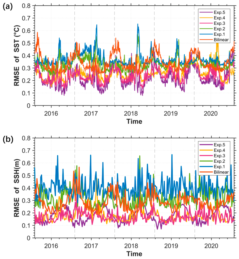
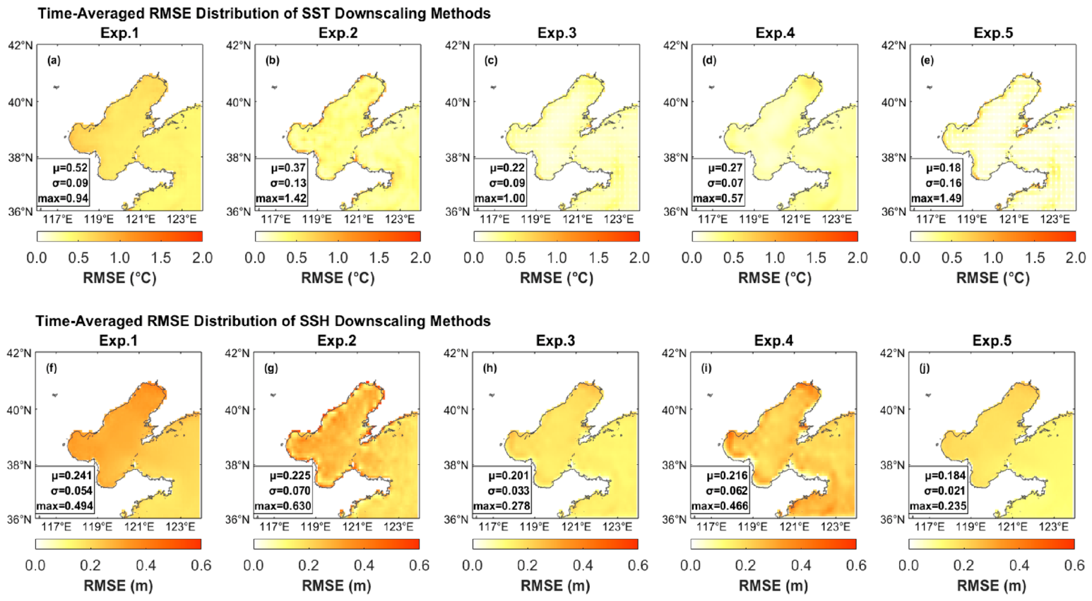
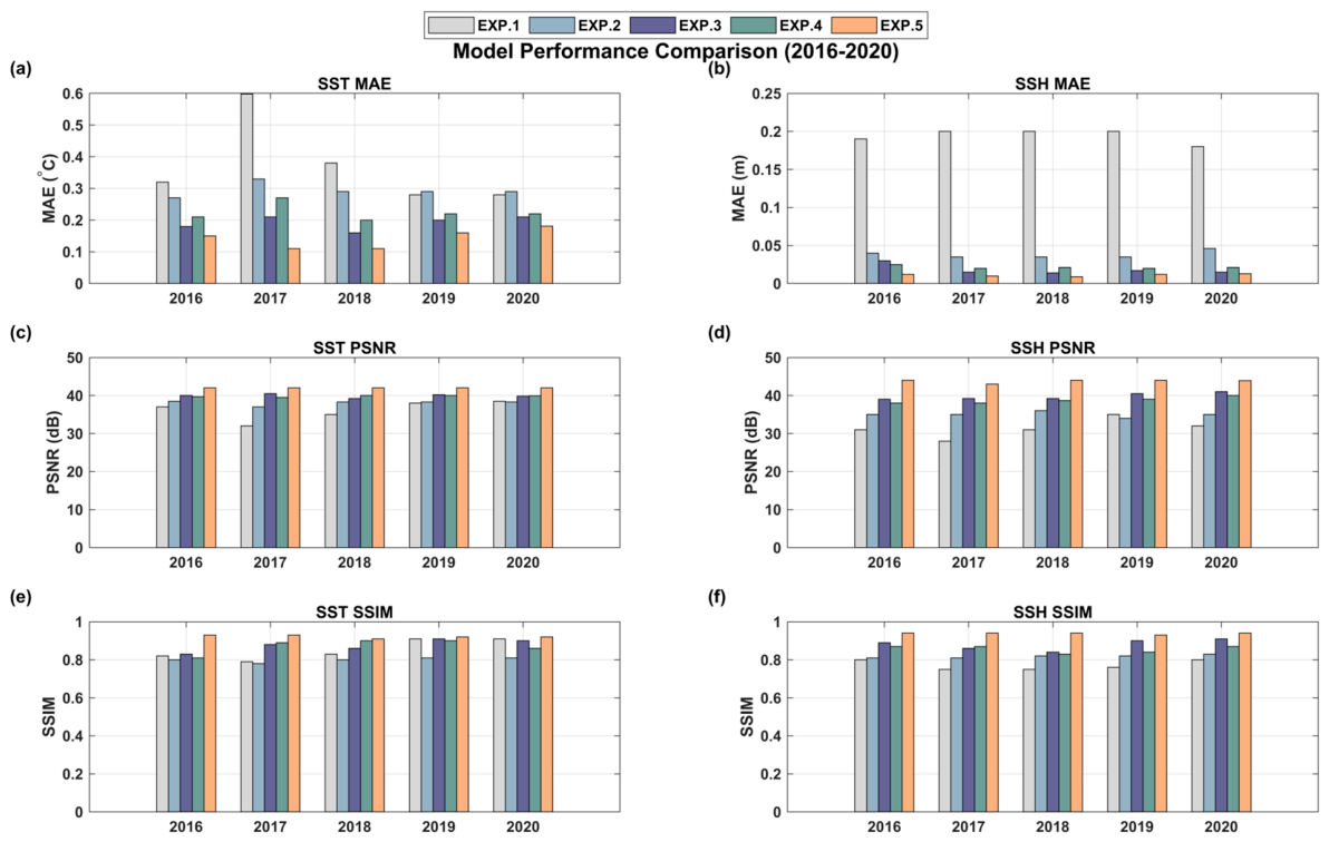
To understand whether different elements support each other during downscaling training, this study discusses the model’s downscaling performance for individual marine variables, as well as the joint downscaling of multiple oceanic variables. Based on four selected model architectures—namely SRGAN, EOFGAN (integrating EOF decomposition with SRGAN), U-NetGAN, and MEOFGAN (integrating MEOF decomposition with SRGAN)—five groups of experiments were designed as summarized in

Table 1. Setup of different experiments in Bohai.

Experiment	Variables	Input Resolution	Model	Output Resolution
Exp.1	SST SSH	1/4°	SRGAN	1/12°
Exp.2	SST SSH	1/4°	EOFGAN	1/12°
Exp.3	SST SSH	1/4°	U-NetGAN	1/12°
Exp.4	SST, SSH	1/4°	MEOFGAN	1/12°
Exp.5	SST, SSH, Bathymetry	1/4°	MEOFGAN	1/12°

.

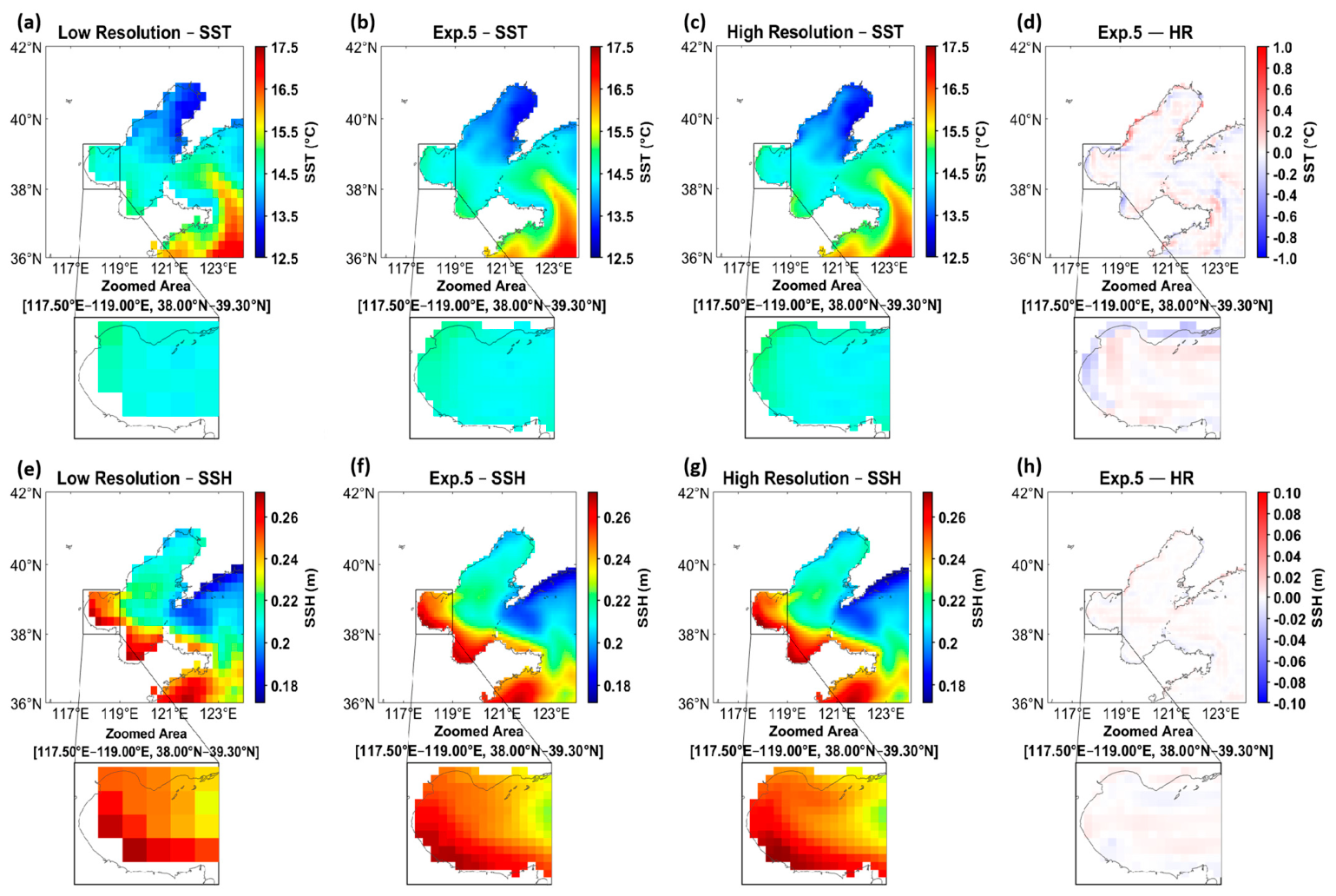
Experiment 1 uses SRGAN as the training module, constructing a framework that directly transitions from low resolution (1/4°) to high resolution (1/12°) for SST and SSH, separately; Experiment 2 maintains the same input and output as Experiment 1 but first performs spatiotemporal decomposition of each marine element based on the EOF method and then simulates the transfer relationship of spatial modes at different resolutions, using EOFGAN as the core neural network module. Experiment 3 also has the same setup as Experiment 1 but replaces the core training module with U-NetGAN to evaluate the impact of different super-resolution network architectures on downscaling performance. Experiment 4 builds upon Experiment 2 by performing multivariate spatiotemporal decomposition of all variables together, constructing spatial modes that include multivariate information and spatial scales, and then using MEOFGAN as the core to learn the relationship between different resolutions. Considering that terrain conditions are correlated during the resolution transition in learning spatial resolution changes, Experiment 5 adds bathymetric data to Experiment 4 to enhance the role of spatial modes in resolution transfer learning.

Considering the relative completeness of dataset for the Bohai Sea area, this study initially conducts experiments on downscaling methods specific to this region. All experiments are conducted using the dataset covering the period from 1993 to 2015, while the dataset from 2016 to 2020 is utilized for independent validation. All datasets were uniformly processed to achieve a daily temporal resolution and spatial alignment. Building on these, the applicability of the method for more refined geographical areas is subsequently explored.

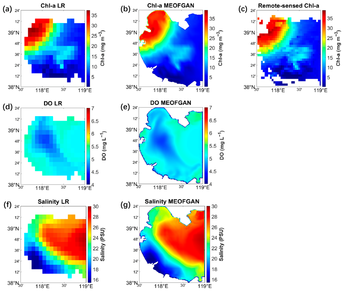
The Bohai Bay (38°–39.4°N, 117.5°–119°E), recognized as a crucial economic and ecological region in China, poses significant challenges for collecting high-resolution environmental data due to its complexity, dynamic nature, and multi-scale characteristics. Therefore, our proposed downscaling method is further tested and applied in the Bohai Bay to simulate environmental factors like Chl-a and DO. Thus, this study concurrently prepared remote sensing data, reanalysis data, and high-resolution numerical model outputs. Considering data availability, the low-resolution observational data in this region are sourced from multiple avenues: Chl-a from satellite observations, DO and salinity from reanalysis products, and bathymetry from the General Bathymetric Chart of the Oceans (GEBCO). All input datasets were standardized to a common spatial resolution of 1/12°. Due to the limited accuracy of remote sensing data in this area, the foundational spatial mode of high-resolution training data is derived from the results of numerical models from previous studies constructed in 2016. Specifically, the high-resolution (500 m) target data for training were obtained from a calibrated Delft3D numerical model for the year 2016 [45]. Utilizing the time-invariant properties of spatial mode, the trained model was applied to the data from 2017, enabling the reconstruction of the corresponding high-resolution data from that year’s low-resolution remote sensing data. The experimental setup is presented in

Table 2. Experimental data configuration for the downscaling model in the Bohai Bay.

Phase	Period	Data Role	Variables	Source and Description	Resolution
Model training	2016	Input (predictors)	Chl-a, DO, salinity, bathymetry	Chl-a: obtained from satellite observations. DO: interpolated from reanalysis products. Salinity: obtained from reanalysis products. Bathymetry: sourced from the General Bathymetric Chart of the Oceans (GEBCO).	1/12° (~8 km)
		Target (high-resolution labels)	Chl-a, DO, salinity, bathymetry	High-fidelity outputs from a calibrated Delft3D numerical model.	500 m
Model validation	2017	Input (predictors)	Chl-a, DO, salinity, bathymetry	Consistent with the training input sources but for the year 2017.	1/12° (~8 km)
		Output (model predictions)	Chl-a, DO, salinity, bathymetry	High-resolution predictions generated by the proposed MEOFGAN model.	500 m

.

4. Results

4.1. Evaluation Metrics

To conduct a comprehensive performance evaluation, we established a multi-dimensional assessment framework. The root mean square error (RMSE) and mean absolute error (MAE) are used to quantify the reconstruction accuracy of the model. The spatial fidelity of the reconstructed field and the preservation of high-resolution details are assessed by two widely adopted metrics, i.e., peak signal-to-noise ratio (PSNR) and structural similarity index (SSIM). These indicators are extensively used in field reconstruction tasks for pixel-level accuracy evaluation, with their mathematical formulations provided below:

$$RMSE=\sqrt{{\displaystyle \frac{1}{L}}\sum _{i=1}^L{\left(X_i-Y_i\right)}^2}$$

(6)

$$MAE={\displaystyle \frac{1}{L}}\sum _{i=1}^L\left|X_i-Y_i\right|$$

(7)

where $X_i$ represents the generated data, $Y_i$ represents the real samples, and $L$ represents the amount of data.

The PSNR, defined as the logarithmic ratio between the maximum signal power and the corrupting noise power, serves as a widely adopted metric for super-resolution performance evaluation. However, its reliance on simple pixel-wise difference calculations fails to adequately correlate with human visual perception. To address this limitation, we incorporate the SSIM, which aligns with the human visual system’s (HVS) sensitivity to structural patterns. By jointly employing PSNR and SSIM, our evaluation framework comprehensively assesses both pixel-level fidelity and perceptual quality of the model’s downscaling results. The mathematical formulations are presented below:

$$PSNR=10\times lg{\displaystyle \frac{I_{max}^2}{MSE}}$$

(8)

$$SSIM={\displaystyle \frac{\left(2{\mu }_X{\mu }_Y+c_1\right)\left(2{\sigma }_{XY}+c_2\right)}{\left({\mu }_X^2{+\mu }_Y^2+c_1\right)\left({\sigma }_X^2{+\sigma }_Y^2+c_2\right)}}$$

(9)

where $I_{max}^2$ represents the maximum value corresponding to the data’s bit depth, which is standardized to 255 for these data; $\mu$ represents the mean; ${\sigma }_X^2$ and ${\sigma }_Y^2$ represent the variances of $X$ and $Y$; ${\sigma }_{XY}$ represents the covariance between $X$ and $Y$; and $c_1$ and $c_2$ are constants. Prior to PSNR and SSIM computation, we normalize the meteorological fields to the [0, 255] range. The SSIM calculation employs a sliding window approach across the entire field, with the final metric obtained by averaging all local window measurements to ensure comprehensive spatial evaluation. The unit of PSNR is dB, where a higher value indicates less distortion. SSIM ranges between 0 and 1, with a higher value indicating greater similarity between the two fields.

4.2. Idealized Experiment on Systematic Bias Propagation

In machine learning-based downscaling, large-scale input data often contain systematic biases. Such biases arise from observation errors, imperfect model parameterizations, or limitations of assimilation strategies and manifest as fixed, non-random tendencies in low-resolution physical variables. If not properly constrained, these biases may be propagated or even amplified by the model to the small-scale outputs. Systematic discrepancies between satellite and in situ measurements are well documented in oceanographic studies. As shown by Boutin et al. [46], these differences originate essentially from near-surface stratification and sub-pixel scale variability. According to comparisons between satellite and Argo sea surface salinity data, the root mean square deviation (RMSD) is approximately 0.2 psu in the open ocean, while significantly larger deviations are observed in coastal regions [47]. To quantitatively assess the risk of such bias propagation, we designed the following idealized bias test solely for SST.

First, we artificially introduced a deterministic and uniform systematic bias into the low-resolution SST data:

$${SST}_{dev}^{LR}= {SST}_{ref}^{LR}+\mathsf{\Delta }$$

(10)

where ${SST}_{dev}^{LR}$ is the low-resolution SST data after introducing the systematic bias, ${SST}_{ref}^{LR}$ is the unbiased low-resolution SST data, and $\mathsf{\Delta }$ is the artificially applied uniform bias. The data with and without the introduced bias are respectively input into different models to compare whether the use of spatial modes as a spatial anchoring template combined with static bathymetry as a constraint can mitigate the propagation of systematic bias. To quantify the degree of error propagation, the error amplification factor (EF) is defined as follows:

$$EF= {\displaystyle \frac{{RMSE}_{out}\left({SST}_{dev}^{HR},{SST}_{ref}^{HR}\right)}{{RMSE}_{in}\left({SST}_{dev}^{LR},{SST}_{ref}^{LR}\right)}}$$

(11)

where ${SST}_{dev}^{HR}$ is the downscaled output corresponding to the biased input, and ${SST}_{ref}^{HR}$ is the downscaled output corresponding to the unbiased input. This metric focuses on evaluating the output bias induced by the input systematic bias, without considering the inherent error of the model itself due to the idealized nature of the test. When $\mathrm{E}\mathrm{F}=1$, the uncertainty is faithfully transferred; when $\mathrm{E}\mathrm{F}>1$, the uncertainty is amplified; when $\mathrm{E}\mathrm{F}<1$, the uncertainty is suppressed, and the smaller the EF value, the more significant the suppression effect.

Table 3. Comparison of EF across different models and bias magnitudes.

Bias (∆)	Model	${\mathbf{RMSE}}_{\mathbf{in}}$	${\mathbf{RMSE}}_{\mathbf{out}}$	EF
0.5	SRGAN EOFGAN MEOFGAN	0.5 0.5 0.5	0.1812 0.1753 0.1694	0.3625 0.3506 0.3387
1.0	SRGAN EOFGAN MEOFGAN	1.0 1.0 1.0	0.3156 0.3029 0.2786	0.3156 0.3029 0.2786
2.0	SRGAN EOFGAN MEOFGAN	2.0 2.0 2.0	0.4935 0.4630 0.4402	0.2468 0.2315 0.2201
5.0	SRGAN EOFGAN MEOFGAN	5.0 5.0 5.0	0.8298 0.8208 0.8177	0.1660 0.1643 0.1635

presents the EF values of the SRGAN, EOFGAN, and MEOFGAN (with SST and bathymetry as inputs) models under different bias magnitudes. The EF values of all three models are below 1, indicating that the models suppress—rather than amplify—the input systematic bias. The monotonic decrease in EF with increasing $∆$ reflects that the output RMSE grows more slowly than the input bias magnitude, demonstrating a favorable error suppression characteristic.

Among the three models, MEOFGAN consistently achieves the lowest EF across all bias magnitudes. At $\mathsf{\Delta }$ = 0.5 °C, the EF of MEOFGAN is 0.3387, compared to 0.3506 for EOFGAN and 0.3625 for SRGAN. At $\mathsf{\Delta }$ = 5.0 °C, the EF of MEOFGAN is 0.1635, compared to 0.1643 for EOFGAN and 0.1660 for SRGAN. MEOFGAN maintains the lowest EF across all $\mathsf{\Delta }$ values, with advantages that are modest in magnitude but consistent in direction. These results confirm that incorporating EOF spatial modes as anchoring templates together with static bathymetric constraints can effectively mitigate the propagation of systematic bias, with MEOFGAN exhibiting the strongest robustness against input uncertainty.

4.3. Evaluation of Downscaling Performance in the Bohai Sea

4.3.1. Temporal and Spatial Assessment of Downscaling Performance

The spatial mean of the RMSEs from the downscaling results of the five proposed experiments during the testing period is illustrated in Figure 5. For comparative purposes, the results of the traditional bilinear interpolation method are also included. As shown in Figure 5a, the estimated errors of SST from Experiment 1 and Experiment 2 are generally comparable to those obtained via bilinear interpolation, fluctuating around 0.35. This indicates that training each individual element separately for downscaling has limited effectiveness, similar to the traditional approach of directly applying bilinear interpolation. However, a closer examination of the results from Experiment 1 and Experiment 2 reveals that the error in Experiment 2 is smaller than that in Experiment 1. This suggests that directly training models using the original time series data of each marine element at different resolutions is less effective than performing EOF decomposition on the respective data and learning their spatial modes. This highlights that the variation in spatial resolution for a marine element primarily depends on its intrinsic spatial characteristics. Effectively separating these spatial features facilitates the analysis of the underlying spatial structure, thereby enhancing the understanding of structural changes in spatial resolution.

Experiment 3, which replaces the core training module with U-NetGAN while maintaining the same input–output setup as Experiment 1, achieves a notable reduction in error, with a spatially averaged RMSE of approximately 0.26 throughout the testing period. This improvement over Experiments 1 and 2 suggests that the U-Net architecture, with its symmetric skip connections, is more effective at preserving spatial details during the downscaling process compared to SRGAN. Notably, Experiment 3 also yields slightly smaller errors than Experiment 4 (which integrates MEOF decomposition without bathymetry) in certain periods, demonstrating the competitiveness of a well-designed single-network architecture.

The results from Experiment 4 and 5 demonstrate a significant reduction in error compared to the outcomes of the other three experiments. In Experiment 4, the spatially averaged RMSE throughout the entire testing period is approximately 0.25. This finding indicates that the integration of multiple oceanic factors for joint downscaling learning effectively captures their varying patterns across different spatial resolutions, thereby reducing estimation errors. This improvement may stem from the joint EOF decomposition of multiple marine elements, which generates spatial modes that encompass not only the spatial structural information of each element but also the interrelations among them. These interrelations provide more intrinsic information for each element during the process of increasing spatial resolution, thus offering a more comprehensive reflection of the changes in high-frequency or short-wavelength data signal characteristics. In Experiment 5, the error stabilizes around 0.2 throughout the entire testing period, yielding results with smaller errors than those of Experiment 4. This interesting result suggests that the integration of bathymetric data into the multivariable spatial modes effectively merges the interrelations and spatial information of each factor with the corresponding bathymetric data. The spatial modes not only incorporate the spatial structural information of each element but also bind the corresponding bathymetric information. Although the bathymetric information itself remains invariant over time, its spatial mode theoretically overlaps with the spatial mode information of each factor. However, when transitioning spatial modes from one scale to another, the inclusion of more explicit bathymetric information facilitates a more effective linkage of the spatial structures of each element across different resolutions, thereby enhancing the clarity of small-scale information and improving the accuracy and efficiency of downscaling learning.

A similar finding can be observed in Figure 5b, where the spatial mean of RMSE for SSH for the proposed experiments are shown. The best performance can be seen in Experiment 5, which confirms that the combination of multiple elements and the integration of bathymetric data contribute to the learning of the transition rules between the spatial structures of various resolutions.

To further elucidate the performance differences among the downscaling methods, we calculated the time-averaged RMSE of the downscaling results for all five experiments over non-land grid points during the test period. As shown in Figure 6, the downscaled SST and SSH results from Experiment 1 exhibit relatively large mean errors across the entire study area, with errors notably increasing toward the coastline and reaching maximum values in nearshore regions. This indicates that applying the SRGAN network alone for downscaling in the Bohai Sea has limited effectiveness. The observed spatial error pattern may be attributed to the learning mechanism of the SRGAN models. Such adversarially trained models tend to prioritize the capture of large-scale, low-frequency signals. Conversely, their ability to accurately represent high-frequency details and small-scale features, which are often prominent in coastal zones, is comparatively weaker. This discrepancy leads to an accumulation of errors in these areas. In this study, the complex and fine-scale coastline of the study area further challenges the model’s capacity to resolve detailed information, resulting in higher errors nearshore. In contrast, offshore regions are more open and data-rich, allowing the model to more effectively capture and represent these features, as reflected in lower errors.

Experiment 3 replaces SRGAN with U-NetGAN as the core training module, achieving further reductions in downscaling errors compared to Experiments 1 and 2. This indicates that the U-Net architecture, with its symmetric skip connections, can more effectively preserve spatial details. Compared to Experiments 1 and 2, Experiment 3 shows particularly pronounced error improvements in nearshore regions. Notably, the overall performance of Experiment 3 is close to—and in some periods, even superior to—that of Experiment 4 (which employs MEOF decomposition without bathymetric data), further demonstrating the competitiveness of the U-Net architecture in single-variable downscaling tasks. Compared with the first four experiments, Experiment 5 achieves a significant reduction in errors, indicating that integrating multiple ocean factors via MEOF decomposition more effectively captures their variation patterns across different spatial resolutions, thereby reducing estimation errors.

Although incorporating bathymetric data in Experiment 5 reduces the mean SST error, it leads to a degradation in maximum error and standard deviation (Figure 6e). Specifically, the maximum error increases sharply from 0.57 in Experiment 4 to 1.49 in Experiment 5, while the standard deviation increases from 0.07 to 0.16. This phenomenon suggests that the integration of bathymetric information does not yield positive effects at all spatial locations. Furthermore, SST and SSH respond differently to the inclusion of bathymetric data: SSH improves consistently across all metrics, whereas SST experiences higher maximum error and standard deviation. This divergence can be attributed to fundamental differences in their physical coupling mechanisms with topography. The dynamic field of SSH is subject to direct and linear constraints from bathymetry (e.g., geostrophic balance, shallow-water wave propagation), and the incorporation of bathymetric data effectively enhances the physical consistency of SSH spatial modes. In contrast, the influence of bathymetry on SST is primarily indirect and nonlinear, mediated through processes such as vertical mixing and upwelling, and is strongly localized. When MEOFGAN attempts to forcibly associate static bathymetric templates with highly dynamic SST modes, overfitting or signal misinterpretation is likely to occur in regions with sharp bathymetric gradients (e.g., coastal corners), leading to localized error amplification.

4.3.2. Quantitative Evaluation of Downscaling Performance

Figure 7 presents a systematic statistical evaluation of the five experimental groups in terms of error and similarity metrics for SST and SSH downscaling tasks over the period from 2016 to 2020.

For SSH downscaling, the annual metrics (MAE, PSNR, SSIM) show stable performance across all years for each experiment, indicating consistent temporal reliability among these five experiments. In comparison with Experiments 2–5, the SRGAN scheme in Experiment 1 tends to produce visually plausible outputs with higher perceptual quality but lower structural accuracy. This indicates that extracting spatial information at different scales from raw data does not necessarily yield stable results. The raw data for each oceanographic element incorporates both spatial variations within the region and temporal evolution over time. In downscaling models, the primary role is played by the spatial information that remains constant over time. Therefore, performing EOF decomposition to separately learn its spatial modes in Experiments 2–5 results in markedly superior outcomes compared to the earlier scheme.

Although superior to Experiment 1, Experiment 2 using EOFGAN still does not adequately capture the cross-variable dependencies between SST and SSH as effectively as Experiments 4–5 due to limitations imposed by its single-variable design. Experiment 3 shows a higher MAE than Experiment 4; nevertheless, it attains equally favorable PSNR and SSIM values, underscoring its capability in retaining spatial details. Experiment 4 achieves an MAE of 0.02 m, outperforming Experiment 2, which uses the EOF method. This demonstrates that the integration of SST and SSH can provide greater spatial coherence through the interconnection of relevant elements, facilitating the incorporation of more effective spatial information within the spatial modality. Notably, Experiment 5, which integrates topographic constraints, consistently reduces errors by approximately 68% and 63% relative to Experiment 4 and Experiment 2, respectively. Its average PSNR reaches 43 dB, and the SSIM is around 0.92, underscoring its effectiveness in detail preservation. This verifies that incorporating bathymetric information can more effectively link spatial modes across varying scales. Such linkage facilitates the transfer of information and training from low-resolution spatial modes to high-scale spatial modes.

A similar finding is observed in SST downscaling results, where Experiment 5 achieves the lowest MAE of below 0.2 °C, representing reductions of approximately 30% and 50% compared to Experiment 4 and Experiment 2, respectively. The PSNR remains consistently around 40 dB, while the SSIM reaches 0.92, demonstrating superior reconstruction of spatial structure.

4.3.3. Comparison of Downscaling Results

Figure 8 presents the downscaling results of SST and SSH over the Bohai Sea from Experiment 5, which enhances the resolution from 1/4° (~25 km) to 1/12° (~8 km). A zoomed-in view of the Bohai Bay is provided to illustrate the capability of MEOFGAN in resolving fine-scale coastal features.

Compared to the low-resolution field, the scheme of MEOFGAN successfully reconstructs spatially continuous SST and SSH distributions, particularly in nearshore regions where the original coarse-grid data contain invalid values due to land–sea mixing. For example, in the Bohai Bay and Laizhou Bay, where the coastline is highly irregular, the downscaled results clearly capture the land–sea thermal contrast and coastal frontal structures during the spring warming period, which are absent in the low-resolution inputs.

In the semi-enclosed Bohai Bay, the proposed MEOFGAN scheme resolves finer-scale SST gradients and SSH variations that reflect the combined effects of shallow bathymetry, seasonal freshwater discharge, and sediment transport. The downscaled SSH field also reveals mesoscale and submesoscale patterns near the Bohai Strait, which are consistent with known circulation features in the region.

In comparison with high-resolution reference data, it can be seen that the results from Experiment 5 preserve the spatial coherence of both SST and SSH while adding physically plausible details. The incorporation of MEOF decomposition allows the model to utilize the coupled variability between SST and SSH, leading to more consistent reconstruction of multivariable structures. Furthermore, the integration of high-resolution bathymetry also helps to maintain topographic constraints on flow and temperature distributions, particularly in shallow coastal regions.

4.4. Evaluation of Downscaling Performance in the Bohai Bay

As previously mentioned, the constructed downscaling model has also been tested in the Bohai Bay for generating higher resolution. As a bay surrounded by industrial cities, this study not only focuses on the physical elements of this region but also further conducts downscaling learning on the low-resolution data of Chl-a and DO present in this area.

4.4.1. Error Analysis of Sub-Kilometer-Scale Downscaling Results

The proposed MEOFGAN downscaling scheme was performed in the Bohai Bay in the testing period of 2016, yielding a high-resolution dataset with a spatial resolution of 500 m. These results are compared with the independent high-resolution target data, and the RMSEs of Chl-a, DO, and salinity in the surface layer are shown in Figure 9.

The proposed scheme, as previously described, essentially makes use of the spatial modes embedded within the data. Due to the time-invariant nature of these spatial modes, the architectural representation of this spatial information remains applicable throughout the independent testing period. Therefore, during this period, high-resolution spatial modes of the region can be reconstructed solely from sparse low-resolution satellite data. These generated spatial modes can subsequently be projected onto the time series, effectively reconstructing a set of high-resolution marine element data that are comparable to the target dataset.

As shown in Figure 9, the proposed EOFGAN scheme successfully generates element information at a resolution of 500 m in the downscaling process for the Bohai Bay. The errors for Chl-a and DO are confined within 0.2–0.3 µg/L and mg/L, respectively, while salinity demonstrates even greater accuracy, with a minimum error region RMSE of only 0.05. This indicates that the two spatial modes employed during the training phase can effectively convey spatial information at two distinct resolutions, and this spatial information remains valid throughout the testing periods.

As can also be observed in Figure 9, the error generally increases toward the coastline. Apart from the GAN model’s preference for large-scale topographic signals, a deeper reason for this phenomenon lies in the inherent spatial mismatch of the data. Both the simulated and satellite data are provided on regular grids, while the actual coastline is a continuous curve. When the coastline traverses or lies immediately adjacent to a grid cell, that cell often contains both water and land, preventing unique assignment of the variable at the grid point. In standard quality control procedures, such mixed grid cells are typically removed, resulting in a systematic absence of valid data in areas neighboring the coastline. Therefore, even if the model possesses sufficient capability, the sparsity and lack of representativeness of training data in nearshore regions still exacerbate error accumulation; in contrast, data in open-ocean regions are continuous and topographically broad, enabling the model to adequately learn large-scale features, with correspondingly smaller errors.

4.4.2. Hindcast Results of Sub-Kilometer-Scale Downscaling Results

To evaluate the applicability of the developed downscaling framework and the trained spatial modes at arbitrary time, the method is applied to a time when only low-resolution real time satellite observations are available. The high-resolution field is then reconstructed using this real-time observation together with the pre-trained spatial modes. According to the annual report, a red tide event occurred in the Bohai Bay from 21 March to 12 April 2017. Therefore, this study selects the satellite observations during this period to conduct downscaling experiments. Considering the potential impacts of the red tide, three representative variables—DO, Chl-a, and salinity—are chosen for the downscaling analysis. The downscaled results on 28 March are shown in Figure 10, where the original satellite data are also presented for comparison.

Compared with the original 4 km satellite product, the 500 m downscaled chlorophyll field exhibits substantially enhanced spatial heterogeneity (Figure 10a–c). The coarse-resolution observation shows rough patterns and fails to distinguish fine structures near the coast, such as river discharge features. In contrast, the downscaled result resolves stronger horizontal gradients and more coherent patches, particularly in shallow coastal waters and around river mouths. These characteristics are consistent with the typical small-scale and patchy nature of red tide events. During the red tide period, the downscaled product provides a clearer depiction of the location and extent of the high-chlorophyll core. Relative to the 4 km data, the reconstructed 500 m field enhances coastal gradients associated with terrestrial input and tidal mixing. Upon further examination of the high-Chl-a area, it can be seen that the 500 m field can present more concentrated high-value areas without excessive spatial diffusion, revealing several secondary patches reflecting the fragmented distribution of the bloom.

Similar results can be observed in Figure 10d,e: compared with the coarse-resolution observation, the reconstructed DO results demonstrate a clear horizontal gradient and more complex and continuous structures. The reduced DO coincides with high-chlorophyll regions in the northeast part, reflecting oxygen consumption caused by algal respiration and organic matter degradation. Some lower DO values tend to appear in the middle of the regions where the Chl-a is not so high; this may be due to the high degree of degradation of organic matter here. From a biogeochemical perspective, the decoupling between low-DO and extremely high-Chl-a patches is ecologically plausible. In mature or declining phases of a red tide, senescent algal cells sink and aggregate, leading to intense microbial degradation at subsurface or bottom layers, which may not directly coincide with surface chlorophyll maxima.

The distribution of salinity is greatly influenced by the river discharge in the south area. As can be seen from Figure 10f,g, the downscaled 500 m salinity field clearly reveals a pronounced gradient from the coastline toward the open sea. Salinity values are significantly lower in the nearshore region and gradually increase offshore, forming a coherent cross-shore transition zone. This pattern is physically consistent with the influence of freshwater discharge from coastal rivers and estuaries, which dilutes surface waters and generates a typical river-plume structure. In comparison, the plume boundaries observed in original coarse-resolution reanalysis data are difficult to identify. After downscaling, the observed sharp frontal zones between coastal and offshore waters effectively reflect mixing processes driven by tides and circulation.

The results from these experiments indicate that the trained spatial modes possess good generalization capability. Given the satellite observation at any time, our proposed downscaling model can construct physically meaningful sub-grid information from low-resolution observations.

5. Discussion

This study is designed to construct a multivariate downscaling scheme to develop high-resolution coastal data by integrating multi-source datasets. In its first application to the Bohai Sea, the multivariate joint downscaling method (MEOFGAN) integrates bathymetric data into multivariable spatial modes and outperforms other experiments. The superior performance highlights the potential of deep learning downscaling methods when using spatial modes as training templates compared to directly training on raw time series data. This underscores that the resolution variations of a marine element are inherently determined by its unique spatial attributes. A clear separation of these spatial features is crucial for analyzing the underlying spatial structure, thereby improving our grasp of how spatial resolution changes structurally. Additionally, adding detailed bathymetry improves how spatial structures link across resolutions. This enhances small-scale details and makes downscaling learning more accurate and efficient.

In data-sparse coastal regions where long-term, high-resolution observations are often unavailable, the application of supervised downscaling methods faces significant challenges. In this study, we trained the downscaling model for the Bohai Sea using daily reanalysis data spanning 28 years from 1993 to 2020. These data are derived from the CMEMS global reanalysis product (GLORYS12V1), which assimilates multi-source satellite observations (including multiple generations of altimeters) and provides physically consistent large-scale dynamical fields. A major advantage of this dataset lies in its coverage of all global ocean areas, including coastal regions, together with excellent spatiotemporal continuity. Our method is inherently a supervised learning approach. Like most supervised downscaling models, its performance is highly dependent on the quality and resolution of the training data. To address this dependency, publicly available high-resolution reanalysis products can serve as effective training targets for coastal zones, providing multi-year data sufficient to obtain stable spatial modes. Furthermore, when existing products are inadequate for specific needs, numerical simulations can be employed to generate customized high-resolution data. In fact, many institutions and projects have already released high-quality, spatially extensive high-resolution public data products that can be directly used as training targets for downscaling models. Meanwhile, the ongoing vigorous promotion of marine and meteorological data-sharing both domestically and internationally will further alleviate data scarcity issues in the future.

The MEOFGAN framework is not a one-size-fits-all model trained once to be applicable to all nearshore areas; rather, it is a general methodological framework that can be flexibly deployed in any target region of interest. Its original design objective does not require zero-shot cross-regional transferability but instead aims to provide a lightweight, efficient, and independently deployable downscaling solution for different coastal zones. By basing the training on spatial modes, the framework substantially reduces computational resource demands while improving computational efficiency. In this study, the eigendecomposition of the spatiotemporal matrix took approximately 12 min on a standard workstation equipped with dual Intel Xeon Gold 6148 CPUs (40 cores) and an NVIDIA RTX A5000 GPU. Subsequent GAN training achieved rapid convergence leveraging GPU parallel computing. In contrast to methods such as SRGAN, which perform super-resolution reconstruction directly on the original spatiotemporal fields and typically require several days of training to achieve stable convergence, MEOFGAN significantly shortens the training time. Specifically, when jointly processing two variables across the entire Bohai Sea, the training took approximately 14 h. When extended to three variables, the training time increased to about 40 h due to the increased dimensionality of the input data. If the study area is reduced to the Bohai Bay, model training can be further reduced to just a few hours. These results indicate that although the computational cost of MEOFGAN increases with the number of variables and the spatial extent, it remains within an acceptable range. Furthermore, its scalability to larger areas can be further enhanced through parallelization strategies [48].

Within the MEOFGAN framework, MEOF decomposition separates a spatiotemporal field into temporally invariant spatial modes and time-varying PCs. The spatial modes represent the statistically optimal covariance structure over the study period and do not change over time; all dynamic variations are fully captured by the PCs. Specifically, the spatial field at any given time is reconstructed as a linear superposition of the same set of spatial modes weighted by the corresponding PC values. This fundamental principle underpins a wide range of ocean forecasting studies, in which a model such as the long short-term memory network (LSTM) [49] is employed to predict the evolution of PCs for forecasting purposes, without the need for frequent recomputation of the spatial modes. It should be noted, however, that while the probability is low that extreme events or rare climatic shifts could lead to fundamental changes in the spatial modes themselves, it is not zero. In such cases, the current framework requires recalculation and updating of the spatial modes.

Based on the above principle, the downscaling results of our model statistically preserve empirical physical relationships among multiple variables (e.g., covariance and correlation structures) but do not pursue strict dynamical consistency that fully satisfies ocean primitive equations or conservation laws. This statistical relationship benefits from two aspects: the reanalysis data inherently embed physical constraints among variables through the data assimilation process, while the MEOF method statistically and explicitly constrains the multivariate covariance structure. In contrast, mainstream deep learning models are essentially purely data-driven “black boxes” that generally lack physical interpretability. Although our method does not achieve dynamical consistency, it already significantly surpasses the practice of conventional deep learning at the statistical level. Future work will be devoted to explicitly incorporating physical constraints, such as momentum and heat, to achieve genuine dynamical consistency.

6. Conclusions

This study integrates the utilization of data from multiple sources and addresses the challenge of reconstructing high-resolution ocean variables in complex coastal regions by proposing a deep learning-based downscaling scheme named MEOFGAN. The model extracts physically interpretable spatial modes of coupled ocean variables, learns their cross-scale transitions through adversarial training, and systematically incorporates high-resolution bathymetry as a static environmental constraint to enhance spatial fidelity. In the application to the Bohai Sea, the model was trained using reanalysis data of SST and SSH to generate corresponding 1/12° fields from 1/4° low-resolution inputs. The results demonstrate that the multivariate spatial modes successfully capture the coupled variability between SST and SSH. Additionally, the integration of bathymetric data further enhances cross-scale consistency. When combined with our deep learning-based downscaling techniques, this scheme enables the enhancement of resolution for existing multivariate datasets.

The scheme was further applied to the Bohai Bay, downscaling Chl-a, DO, and salinity data from 1/12° to 500 m resolution. Despite the differences in data sources and variable types, the MEOFGAN framework successfully reconstructed fine-scale spatial gradients and continuous structures that were indiscernible in the original satellite data. A key advantage of this method lies in its ability to identify intrinsic covariability patterns among multiple variables while achieving efficient dimensionality reduction through spatiotemporal orthogonal basis functions, thereby significantly enhancing computational efficiency in processing large-scale oceanographic datasets. This capability fully exploits the potential of available data, compensates for the resolution limitations of coastal remote sensing, and provides the fine-scale information required for coastal environmental applications.

Overall, the MEOFGAN scheme offers a lightweight and efficient pathway for reconstructing high-resolution coastal ocean elements, directly addressing the challenge of insufficient fine-scale observational capabilities in dynamic nearshore regions. The method not only enhances the utility of existing limited-resolution datasets but also provides a scalable technical route toward constructing higher-accuracy coastal datasets, thereby robustly supporting advanced applications such as regional forecasting, ecosystem management, and climate adaptation planning in high-risk maritime zones.