An Intelligent Gated Fusion Network for Waterbody Recognition in Multispectral Remote Sensing Imagery

Highlights

What are the main findings?

• This study proposes a novel Intelligent Gated Fusion Network (IGF-Net). The dual-branch feature encoder is designed to alleviate the input channel mismatch between pre-trained RGB models and multi-band data. Its core Intelligent Gated Fusion Module (IGFM) facilitates adaptive fusion of spectral and visual features.
• Extensive experiments indicate that IGF-Net achieves highly competitive performance (IoU: 0.8742, Dice: 0.9239) on the newly constructed dataset and shows favorable generalization on an independent Sentinel-2 dataset, performing competitively compared with mainstream segmentation models.

What are the implications of the main findings?

• The work provides an effective and robust deep learning solution for accurate water body recognition from multispectral imagery, which can directly benefit practical applications such as hydrological monitoring, environmental management, and disaster assessment.
• We construct and publicly release the “Tiangong-2 Remote Sensing Image Water Body Semantic Segmentation Dataset” along with the complete model implementation code, offering a valuable benchmark and reproducible research foundation for the community.

Abstract

Accurate water body segmentation from multispectral remote sensing imagery is critical for hydrological monitoring and environmental management. However, leveraging transfer learning with pre-trained models remains challenging due to the dimensional mismatch between three-channel RGB-based architectures and multi-band spectral data. To address this, this study proposes a novel segmentation network, termed Intelligent Gated Fusion Network (IGF-Net), built upon a dual-branch feature encoder module and a core Intelligent Gated Fusion Module (IGFM). The IGFM achieves adaptive fusion of visual and spectral features through a cascaded mechanism integrating differences-and-commonalities parallel modeling, channel-context priors, and adaptive temperature control. We evaluate IGF-Net on the newly constructed Tiangong-2 remote sensing image water body semantic segmentation dataset, which comprises 3776 meticulously annotated multispectral image patches. Comprehensive experiments demonstrate that IGF-Net achieves strong and consistent performance on this dataset, with an Intersection over Union of 0.8742 and a Dice coefficient of 0.9239, consistently outperforming the evaluated baseline methods, such as FCN, U-Net, and DeepLabv3+. It also exhibits strong cross-dataset generalization capabilities on an independent Sentinel-2 water segmentation dataset. Ablation studies and visualization analyses confirm that the proposed fusion strategy significantly enhances segmentation accuracy and stability, particularly in complex scenarios. Placeholder.

1. Introduction

Water bodies constitute the general designation for water aggregates including rivers, lakes, and oceans. Rapid and accurate identification of water bodies from remote sensing imagery holds significant practical value for applications such as flood prediction, coastline monitoring, water resource evaluation, and agricultural planning. The extraction of water body information from remote sensing data through digital image processing techniques represents a crucial research focus within the field of remote sensing applications. Relevant scholars in this domain have developed multiple water body recognition methodologies, which can be systematically classified into three primary categories: traditional methods, machine-learning-based methods, and deep-learning-based methods.

Traditional methods primarily include visual interpretation and water index approaches. Among these, visual interpretation refers to the process where experts identify water body areas by observing differences in color and shape of features within remote sensing imagery. While offering high accuracy, this method heavily depends on expert experience and is labor-intensive, leading to low efficiency. Water index methods leverage the spectral characteristics of water bodies to construct mathematical models through band selection in remote sensing imagery. Threshold segmentation is then applied to achieve land-water separation. Commonly used water indices include the Normalized Difference Water Index (NDWI) [1], Revised Normalized Difference Water Index (RNDWI) [2], Shadow Water Index (SWI) [3], and Enhanced Water Index (EWI) [4]. Different indices are suitable for distinct application scenarios; for instance, EWI performs better in semi-arid regions, while SWI is more applicable to mountainous water bodies.

Machine-learning-based methods for water body identification first require manual feature selection. These features can be regarded as abstract representations of water body information within remote sensing imagery. Subsequently, machine learning classifiers use these features during training. Once trained, the classifiers can rapidly identify water body pixels in remote sensing imagery based on these features. Commonly used classifiers include decision trees [5], support vector machines [6], and other algorithms. Compared to water index methods, machine learning approaches typically achieve higher identification accuracy. However, their performance heavily depends on feature selection, and such methods often exhibit limited generalization capability.

Following the breakthrough of AlexNet [7] in the 2012 ImageNet [8] competition, deep learning methods have rapidly advanced and have been extensively applied to water body identification tasks in remote sensing imagery. These methods typically rely on large volumes of annotated samples to train neural networks for the accurate identification of water pixels. Generally speaking, existing research has proceeded along two primary trajectories: one focusing on water body extraction in challenging scenarios, enhancing adaptability to boundary ambiguity, shadow interference, complex backgrounds, and cross-regional variations through network architecture improvements; the other emphasizing multispectral information utilization by integrating non-visible bands (e.g., NIR and SWIR) to enhance the model’s discriminative capabilities between water and non-water features.

Regarding water extraction in complex scenarios, researchers have undertaken extensive structural optimization efforts targeting specific application contexts. For instance, to tackle the challenges of subtle spectral/spatial feature differences between water bodies and background, blurred boundaries, and difficulties in extracting small water bodies within tidal flat environments, Zhang et al. developed FYOLOv3. This approach accomplishes fine-grained extraction of tidal flat water bodies through enhancements to YOLOv3, incorporating both a pooling-free fully convolutional network architecture and pixel-wise similarity discriminative mechanisms [9]. To address the inadequacies of baseline semantic segmentation models in complex remote sensing imagery and the challenge of blurred water body boundaries, Weng et al. developed a U-Net-based framework incorporating the Object Context module, while integrating Atrous Spatial Pyramid Pooling (ASPP) and self-attention mechanisms. This architectural design enhances multi-scale contextual feature extraction capabilities and improves water boundary segmentation accuracy [10]. In ultra-high spatial resolution urban scenarios, Li et al. conducted a systematic evaluation of the water body extraction efficacy of a fully convolutional network (FCN) under constrained training sample conditions. The experimental results demonstrate that this FCN-based approach effectively leverages spatial contextual information to differentiate water bodies from shadow regions, achieving overall performance superiority over benchmark methods including NDWI and SVM [11]. In the context of global-scale water body identification, Isikdogan et al. introduced DeepWater Map, which formulates water extraction as a multi-scale fully convolutional semantic segmentation framework. This methodology significantly reduces the dependence of conventional spectral-index-based approaches on empirically determined thresholds while simultaneously minimizing misclassification errors associated with snow, ice, cloud cover and shadowed regions [12]. To tackle challenging interference conditions in agricultural watersheds including shadow effects, water quality variability, and vegetation occlusion, Liao et al. developed a lightweight architecture termed LKF-DCANet. This framework utilizes deformable convolutions for adaptive geometric feature extraction of water bodies, while incorporating learnable Kalman filtering during feature decoding for denoising. While maintaining a compact parameter footprint, the approach demonstrates competitive segmentation performance, with additional gains achieved through subsequent knowledge distillation [13]. The EU-Net developed by Cao et al. strengthens multi-scale contextual modeling through dilated convolutions at multiple scales, attention mechanisms, and enhanced residual connections. This architecture integrates multi-scale feature fusion to deliver superior boundary segmentation accuracy, particularly for extracting complex-textured water bodies, small-scale aquatic features, and narrow channel regions [14]. To address the paucity of labeled samples for small water body delineation in sub-meter resolution satellite imagery, Li et al. established a cross-sensor transfer learning framework bridging Sentinel-2 and PlanetScope datasets. Their systematic evaluation of the state-space model VMamba demonstrates its promising potential for small water body mapping, thereby providing an innovative computational approach for precise extraction of hydrological features from ultra-high-resolution imagery [15].

Conversely, non-visible-band spectral information from multispectral remote sensing imagery, particularly NIR and SWIR, substantially enhances spectral discrimination capabilities for water-body identification. A comparative investigation by Ngo et al. utilizing unmanned aerial vehicle-acquired multispectral data demonstrated that fusing ancillary features including NIR reflectance and NDWI yields statistically significant improvements in water detection and segmentation accuracy within complex humid tropical ecosystems, outperforming RGB-only input configurations [16]. Building upon these insights, researchers have developed multiple fusion-based segmentation networks specifically designed for multispectral information utilization. Weng et al. introduced SCR-Net, which employs a four-band RGB + NIR input configuration within a dual-branch encoder-decoder framework. This architecture utilizes a ConvFormer branch for global context modeling, while integrating a ResNet-50-based residual pathway with a GAM channel-spatial attention mechanism to enhance feature representation and detail delineation. This design enables effective multispectral information fusion and fine-scale water body segmentation [17]. To tackle the challenge of heterogeneous spatial resolutions across Sentinel-2 multispectral bands and feature degradation induced by conventional interpolation-based upsampling, Yuan et al. developed an end-to-end multi-channel water body detection network named MC-WBDN. This architecture performs front-end fusion of RGB, NIR, and SWIR spectral bands while integrating enhanced atrous spatial pyramid pooling modules. The proposed approach significantly enhances multispectral water segmentation accuracy and robustness against illumination variations and atmospheric disturbances, demonstrating particular efficacy in detecting micro-scale hydrological features [18]. To tackle the challenges of spectral reflectance instability in complex aquatic environments and interference from reflections, ripples, and specular highlights, Hu et al. developed a shape-spectrum fusion-based water detection approach leveraging multi-frame multispectral imagery. The methodology establishes a dual-path feature extraction architecture with separate spectral-spatial processing streams. In the spectral pathway, temporal-spectral fusion significantly reduces water-surface dynamic disturbances, while channel-wise and spatial attention mechanisms are synergistically embedded in both the spatial branch and fusion stages, achieving high-precision and robust pixel-level water segmentation [19]. Beyond multispectral information, researchers have incorporated active-mode microwave remote sensing data (e.g., SAR) to develop multi-source/multi-modal fusion approaches, aiming to enhance water segmentation and recognition capabilities in challenging environments. To overcome the inherent limitations of standalone optical or microwave remote sensing data for small water body identification in rugged terrain regions, Yang et al. introduced a multispectral-SAR image fusion algorithm named MASF. This method successfully accomplishes synergistic fusion of both data modalities through a multi-resolution analytical framework. By subsequently integrating spectral, textural, and geometric features with multi-scale segmentation and RF-based classification, the approach achieves precise delineation of small water bodies in complex topographic settings [20]. Wang et al. developed MFGF-UNet and established the WIPI multimodal dataset, which synthesizes Sentinel-2 water-index-derived features with Sentinel-1 polarimetric information. The architecture incorporates a gated multi-scale filter Inception module and channel-wise attention-based GCT skip connections, significantly improving multi-scale water body feature representation. This approach exhibits superior segmentation accuracy and generalization capability across diverse benchmarks (WIPI, Chengdu, GF2020) while maintaining high parameter efficiency [21]. In addition, related studies in other vision tasks have also explored attention mechanisms and feature enhancement strategies to improve boundary representation and robustness under complex backgrounds [22].

Collectively, contemporary deep learning approaches have demonstrated substantial advancements in both scenario adaptability and multispectral information utilization. Notably, multi-spectral fusion segmentation networks have validated that non-visible-band spectral data significantly enhances water-body identification efficacy under complex environmental conditions. For systematic comparison of the aforementioned representative methodologies,

Table 1. Comparison of representative remote sensing water body identification methods.

Representative Method	Input Type	Key Architecture	Main Strengths
Weng et al.: SCR-Net [17]	RGB + NIR	ConvFormer branch + ResNet-50 branch + GAM attention module	Balances global context and local details for effective multispectral fusion and accurate water body segmentation.
Yang et al.: Multispectral and SAR Fusion algorithm [20]	Multispectral + SAR	MASF + multi-scale segmentation + random forest	Fuses complementary multispectral and SAR information to identify fragmented small water bodies in complex terrain.
Wang et al.: MFGF-UNet [21]	SAR and the seven water indexes	U-Net + gated multi-filter inception module + GCT skip connection	Leverages multimodal and multiscale features for strong, robust, and low-complexity performance on the WIPI, Chengdu, and GF2020 datasets.
Liao et al.: LKF-DCANet [13]	RGB	Channel attention-enhanced deformable convolution module + convolutional additive token mixer + learnable Kalman filter	Achieves precise boundary delineation and strong robustness to noise and appearance ambiguity with only 0.22 M parameters.
Cao et al.: EU-Net [14]	RGB + NIR	Improved residual connections + multi-scale dilated convolution module + multi-scale feature fusion module + channel and spatial attention mechanisms	Maintains water-body geometry and clear boundaries, especially in small water bodies, narrow channels, and complex scenes.
Li et al.: transfer learning framework from Sentinel-2 to PlanetScope [15]	RGB + NIR	Transfer learning framework from Sentinel-2 to PlanetScope + assessment of VMamba for small water-body mapping	Reduces manual annotation effort and improves small water body mapping in cross-sensor transfer learning.

synthesizes their principal input modalities, core architectural designs, and distinctive methodological features. Comprehensive analysis of Table 1 reveals persistent common limitations across current approaches. In terms of fusion strategies, contemporary approaches predominantly employ conventional paradigms involving unified multi-band inputs or channel-level concatenation. While these methods enable partial integration of multi-source information, they critically lack explicit differentiation between the distinct learning objectives associated with visible and non-visible-band spectral modalities. This fundamental limitation severely constrains the potential synergy that could be derived from the complementary characteristics of these two data domains. For example, while SCR-Net employs a dual-branch architecture, both branches process identical four-channel RGB + NIR inputs. The distinction between branches predominantly manifests in their architectural configurations and targeted feature modeling strategies, rather than through explicit input-modality-based processing objective separation [17]. While MFGF-UNet implements enhancements in attention mechanisms and multi-scale feature modeling via GCT skip connections and the GMF-Inception module, its cross-modality fusion strategy fundamentally operates by organizing pre-extracted water indices and SAR polarimetric features into input-stage multi-channel representations. These are subsequently processed through a shared backbone network, thereby remaining fundamentally within the unified fusion paradigm characterized by channel-wise concatenation [21]. From the viewpoint of pre-trained knowledge utilization, multispectral/multimodal inputs and their purpose-built fusion architectures exhibit fundamental incompatibility with the conventional RGB-based pre-training paradigm established in natural image processing. This inherent discrepancy frequently prevents direct reuse of mature pre-trained representations in adapted model architectures. Prominent approaches like LKF-DCANet [13] and EU-Net [14] remain fundamentally grounded in optical image segmentation frameworks, directing primary research efforts toward spatial feature augmentation, contextual modeling, and network architecture lightweighting. Consequently, these methods fail to establish explicit spectral decoupling and fusion mechanisms specifically designed for multispectral bands. Specifically, while LKF-DCANet exclusively employs RGB optical imagery for experimental validation, EU-Net—despite being tested on high-resolution optical data containing NIR bands—does not methodologically emphasize multispectral information modeling in its architectural innovations. While the cross-sensor transfer learning framework developed by Li et al. [15] successfully addresses sample scarcity challenges in high-resolution small water body mapping, its input organization maintains a consolidated four-band RGB-NIR configuration lacking explicit spectral decoupling and spectral-interaction modeling mechanisms. This highlights a critical research gap: simultaneously preserving RGB pre-training benefits through explicit separation of visible/non-visible-band learning pathways, while enabling bi-directional adaptive feature interaction across modalities—both remaining fundamental challenges in multispectral remote sensing water segmentation.

To address this issue, this study proposes an Intelligent Gated Fusion Network (IGF-Net). Our dual-branch encoder processes synthetic RGB images (from selected RGB bands) in one branch for generic visual representation, while the complementary branch mines unique spectral patterns from non-visible bands. An adaptive gating mechanism dynamically modulates cross-branch feature interactions, prioritizing channel-wise discriminative cues through learnable weights. This study follows a complete workflow covering data processing, model construction, and systematic experimental validation. Preprocessing is first performed on the multispectral remote sensing image dataset. Next, a segmentation network centered on a Dual-Branch Feature Encoder Module and an Intelligent Gated Fusion Module (IGFM) is constructed. Finally, model performance is evaluated through comparative experiments against mainstream methods and ablation studies with replaced fusion modules. The remainder of this paper is organized as follows: Section 2 introduces the dataset characteristics and preprocessing protocol. Section 3 systematically elaborates on the architecture and implementation details of the proposed intelligent gated fusion network. Section 4 presents the complete experimental setup and result analysis. Section 5 concludes the paper and provides an outlook for future work.

2. Dataset

To comprehensively evaluate the performance and generalization capability of the proposed model, this study employs two multispectral water body semantic segmentation datasets: (1) a custom-built Tiangong-2 remote sensing dataset with water body annotations, and (2) the publicly released Sentinel-2 Water Segmentation Dataset introduced by Yuan et al. [18]. Subsequent sections present detailed descriptions of both datasets.

2.1. Tiangong-2 Remote Sensing Image Water Body Semantic Segmentation Dataset

The multispectral data used in the Tiangong-2 Remote Sensing Image Water Body Semantic Segmentation Dataset originate from the “Tiangong-2 Remote Sensing Image Natural Scene Classification Dataset” [23]. This dataset was developed through systematic consideration of critical factors including geographic diversity and temporal coverage. It comprises two primary components: (1) multispectral imagery with 14 discrete spectral bands spanning 0.403–0.990 μm, encompassing both visible and near-infrared regions, and (2) corresponding RGB true-color composites generated from specific bands (7, 11, and 12). The non-contiguous spectral sampling across this range is designed to enhance the differentiation of surface features, including water bodies. Complete specifications of individual band wavelengths are provided in

Table 2. Spectral band specifications of the Tiangong-2 Remote Sensing Image Natural Scene Classification Dataset.

Channel Number	Spectral Range (μm)
V1	0.970–0.990
V2	0.930–0.950
V3	0.895–0.915
V4	0.845–0.885
V5	0.810–0.830
V6	0.740–0.760
V7	0.6775–0.6875
V8	0.655–0.675
V9	0.610–0.630
V10	0.555–0.575
V11	0.510–0.530
V12	0.480–0.500
V13	0.433–0.453
V14	0.403–0.423

Note: Band specifications were compiled from the dataset metadata of the Tiangong-2 Remote Sensing Image Natural Scene Classification Dataset (V1).

.

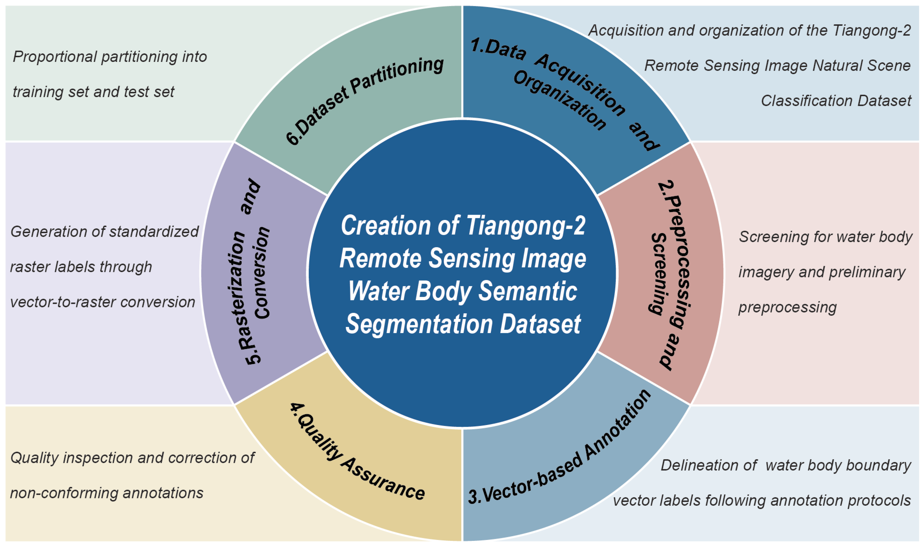
A total of 3776 images containing water bodies were selected from the aforementioned dataset. Based on this subset, we established the “Tiangong-2 Remote Sensing Image Water Body Semantic Segmentation Dataset” through manual visual interpretation. The annotation procedure employed the LabelMe tool to precisely delineate surface water bodies [24]. Annotated results were converted into binary raster labels (TIFF format) using a custom-developed Python (v3.10.18) script. In these label images, water body pixels are assigned a grayscale value of 255 (maximum intensity), while background pixels are assigned 0 (minimum intensity). To optimize data access efficiency, all original multispectral images in TIFF format were systematically transformed into NPY format—a specialized extension for NumPy that enables efficient loading of multi-dimensional arrays. After completing the aforementioned preprocessing, the dataset was randomly partitioned into a training set (3402 images) and a test set (374 images) at a 9:1 ratio. The complete data preparation pipeline is depicted in Figure 1.

2.2. Sentinel-2 Water Segmentation Dataset

To ensure fair comparison with existing representative methods and validate the model’s generalizability on a public benchmark, this study adopts the publicly released Sentinel-2 Water Segmentation Dataset by Yuan et al. [18]. The dataset encompasses Chengdu City, Sichuan Province, China, along with its adjacent peri-urban transitional zones, utilizing Sentinel-2 satellite imagery. Notably, all training, validation, and quantitative testing in this study strictly employ the first temporal phase data (April 2018). While the original study primarily utilized the second (December 2018) and third (February 2019) phases as cross-temporal images to assess model robustness under varying illumination and weather conditions, we repurpose these phases exclusively for visual analysis in multi-temporal experiments.

To ensure spatial alignment among the multi-band data and compliance with network input specifications, the following preprocessing steps were applied:

(1)

Spatial Resolution Unification: Given the lower spatial resolution of SWIR bands (typically 20 m for Sentinel-2) compared to RGB/NIR bands (10 m), bilinear interpolation was applied to upsample SWIR data to 10 m, ensuring consistent spatial scale across all bands.

(2)

Image Cropping and Tiling: A grid-based cropping method was employed to divide the resolution-unified multi-band images into non-overlapping square patches of size 256 × 256 pixels.

(3)

Dataset Splitting: In accordance with the 9:1 ratio established for the custom-built dataset, all valid image patches were randomly partitioned into training and test sets.

These preprocessing steps resulted in a curated collection of standardized image patches, ready for model input and subsequent analysis.

2.3. Comparison of the Two Datasets

Significant differences exist between the Tiangong-2 Remote Sensing Image Water Body Semantic Segmentation Dataset and the Sentinel-2 Water Segmentation Dataset regarding data sources, sensor platforms, spectral characteristics, and experimental purposes. Specifically, the former is a custom-built dataset constructed from Tiangong-2 multispectral imagery through manual annotation, containing 14 spectral bands (detailed in Table 2), primarily used to evaluate the proposed method’s effectiveness on the custom-built multispectral data. The latter is a publicly available benchmark dataset derived from Sentinel-2 imagery, encompassing visible, near-infrared, and shortwave infrared bands, mainly employed to validate the proposed model’s performance on a standardized public benchmark as well as its cross-temporal generalization capability. A detailed comparison of the two datasets is presented in

Table 3. Comparison between the Tiangong-2 Remote Sensing Image Water Body Semantic Segmentation Dataset and the Sentinel-2 Water Segmentation Dataset.

Aspect	Tiangong-2 Remote Sensing Image Water Body Semantic Segmentation Dataset	Sentinel-2 Water Segmentation Dataset
Data source	Custom-built from the Tiangong-2 Remote Sensing Image Natural Scene Classification Dataset.	Public dataset released by Yuan et al.
Spectral characteristics	14 discrete spectral bands spanning 0.403–0.990 μm.	Multispectral imagery including RGB, NIR, and SWIR bands.
Annotation strategy	Manually annotated in this study using LabelMe.	Labels provided in the original public benchmark dataset.
Data preparation	TIFF images converted to NPY format; binary labels generated by a custom script.	SWIR bands upsampled from 20 m to 10 m and cropped into 256 × 256 patches.
Temporal setting in this study	Used for supervised training and quantitative evaluation.	April 2018 data used for training, validation, and quantitative testing; December 2018 and February 2019 data used for qualitative visual analysis.
Primary role in this study	Task-specific evaluation on a custom-built multispectral dataset.	Benchmark evaluation and cross-temporal generalization analysis on a public dataset.

.

For clarity, the Tiangong-2 Remote Sensing Image Water Body Semantic Segmentation Dataset is abbreviated as TG2-WaterSeg, and the Sentinel-2 Water Segmentation Dataset is abbreviated as S2-WaterSeg in the remainder of this paper.

3. Methodology

3.1. Intelligent Gated Fusion Network Architecture

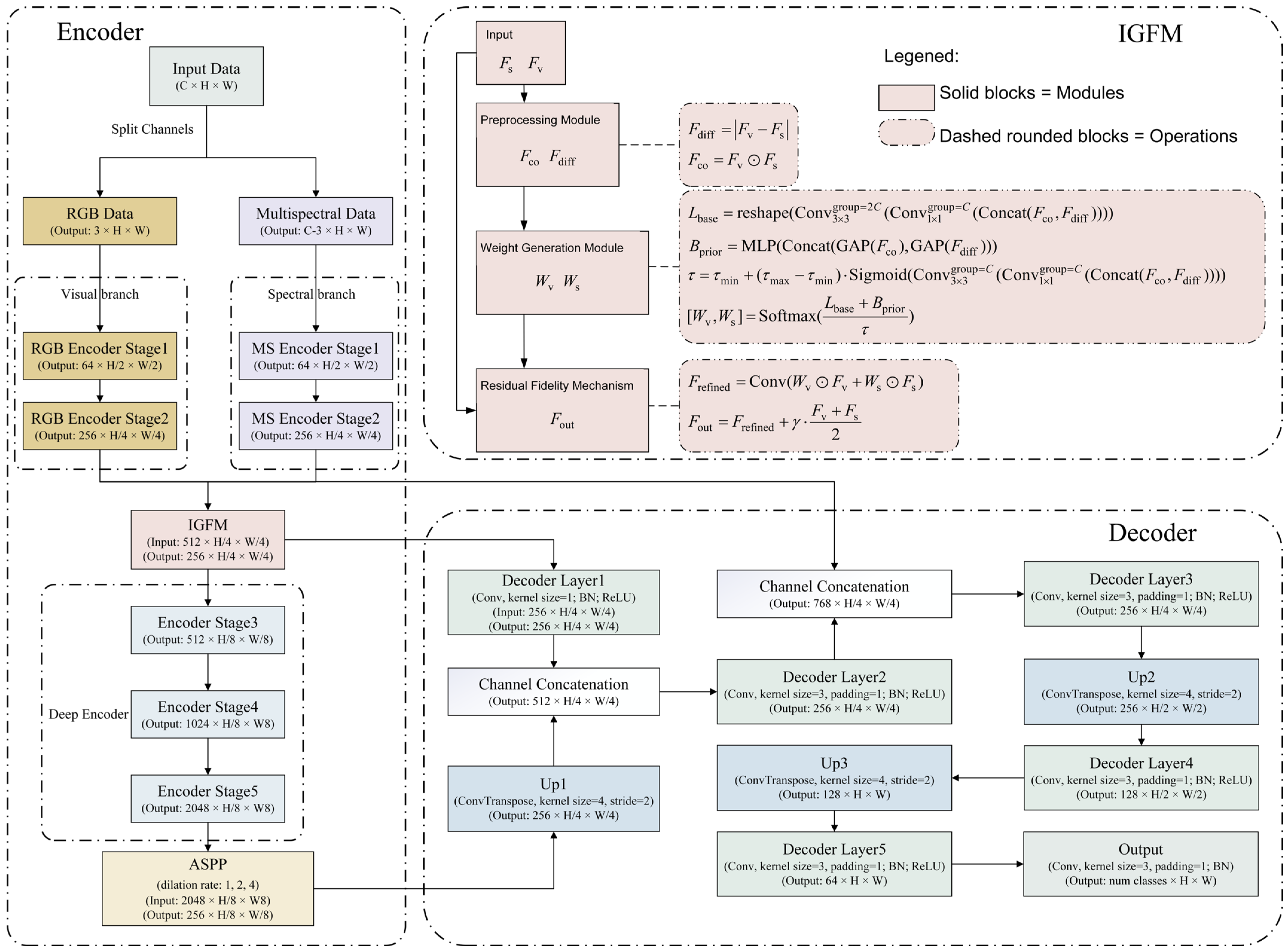
To tackle the challenges of water body segmentation in multispectral remote sensing imagery, this study proposes an end-to-end IGF-Net. The network adopts an encoder-decoder architecture [25], taking multispectral images as input and generating corresponding binary segmentation masks for water bodies as output. The overall structure of the network is illustrated in Figure 2.

As the feature extraction core of the model, the encoder is comprised mainly of the following three modules:

(1)

Dual-Branch Feature Encoder Module: This module employs a parallel dual-branch structure to process distinct band subsets of the multispectral data. The visual branch takes the red, green, and blue bands as input and loads weights pre-trained on ImageNet to extract general visual features. The spectral branch processes the remaining bands with randomly initialized weights, specializing in learning spectral-specific features from the multispectral data. Both branches adopt the ResNet-50 backbone [26], producing feature maps at 1/4 of the input spatial resolution with 256 channels.

(2)

Intelligent Gated Fusion Module: As the core innovation of this study, this module receives outputs from the dual-branch feature encoder. Through a gating-based adaptive mechanism, it dynamically learns branch-wise attention weights via trainable parameters, enabling selective fusion of visual and spectral features to enhance the model’s focus on key discriminative characteristics.

(3)

Atrous Spatial Pyramid Pooling (ASPP) Module [27]: Following further processing by the deep encoder, the fused features are passed to the ASPP module. This module aggregates multi-scale contextual information through parallel atrous convolutions with varying dilation rates, thereby strengthening the model’s capacity to capture water bodies across diverse spatial scales.

The decoder employs a progressive upsampling scheme with multi-level feature fusion. It first processes the high-level semantic features from the encoder, reducing their dimensionality via a 1 × 1 convolution and then upsampling them to a quarter of the input resolution. These upsampled features are then fused—via skip connections—with shallow features from the Intelligent Gated Fusion Module, the visual branch, and the spectral branch, integrating complementary spatial details. Finally, through two consecutive upsampling stages (each doubling the resolution), each refined by 3 × 3 convolutions, the feature maps are restored to the original input resolution to yield high-precision segmentation predictions.

To clearly present the technical details of the model and ensure the reproducibility of the research, the detailed parameter settings and inter-layer connections of the network are provided in

Table 4. Description of the Intelligent Gated Fusion Network architecture.

Stage/Module		Input Size	Output Size	Details
Input Data		C × H × W	(C-3) × H × W and 3 × H × W	Split the input into RGB and multispectral data by channel indices.
Encoder	Visual branch Encoder	3 × H × W	256 × H/4 × W/4	Extract RGB features using a shallow ResNet50 encoder with pretrained initialization.
	Spectral branch Encoder	(C-3) × H × W	256 × H/4 × W/4	Extract multispectral features using a shallow ResNet50 encoder with random initialization.
	IGFM	512 × H/4 × W/4	256 × H/4 × W/4	Adaptively fuse dual-branch features with dynamic weights while preserving residual information.
	Deep Encoder	256 × H/4 × W/4	2048 × H/8 × W/8	Further extract high-level semantic features using the deep ResNet50 encoder.
	ASPP	2048 × H/8 × W/8	256 × H/8 × W/8	Extract multi-scale contextual features through parallel convolutions with different dilation rates.
Decoder		ASPP: 256 × H/8 × W/8; IGFM: 256 × H/4 × W/4; RGB Encoder Stage2: 256 × H/4 × W/4; MS Encoder Stage2: 256 × H/4 × W/4	Num classes × H × W	Generate the final prediction result via transposed convolution upsampling, channel concatenation, and convolutional refinement.

.

3.2. Dual-Branch Feature Encoder Module

Transfer learning, by leveraging parameters from models pre-trained on large-scale datasets (e.g., ImageNet), significantly enhances both model performance and training efficiency for target tasks. However, applying this methodology to multispectral remote sensing image segmentation encounters a critical issue: prevalent pre-trained architectures (such as ResNet-50) are inherently designed for three-channel color images, with their input dimensions strictly confined to three channels. When processing multispectral data containing more than three spectral bands, this channel dimension discrepancy precludes direct initialization with pre-trained weights, thus diminishing the efficacy of transfer learning.

To address the aforementioned challenge, our model employs a dual-branch feature encoder module. This architecture comprises two distinct branches built upon the ResNet-50 backbone: a visual branch and a spectral branch. The visual branch processes the three specific bands (red, green, blue) from the input multispectral data, initializing with weights pre-trained on ImageNet. This design enables direct transfer of generic visual features (such as edges and textures) acquired from large-scale datasets, endowing the model with robust spatial semantic priors. Conversely, the spectral branch handles all residual spectral bands (excluding RGB channels), maintaining identical architectural configuration to the visual branch but utilizing randomly initialized weights. Specialized for multispectral analysis, this branch captures minute reflectance variations among different land cover categories across extensive spectral ranges.

The design of this dual-branch feature encoder module is founded on a principle of explicit complementarity. The visual branch inherits the robust generic feature representation from pre-trained models, while the spectral branch confers specialized learning capacity for multispectral signatures. This separate encoding strategy simultaneously harnesses the benefits of transfer learning and avoids the structural conflicts or information loss associated with forced input dimensionality alterations. Consequently, the module provides dual feature representations for downstream fusion, incorporating both general visual knowledge and domain-specific spectral information.

3.3. Intelligent Gated Fusion Module

The fusion quality of features extracted by the dual-branch feature encoder module critically determines the final segmentation performance. Since the visual branch and the spectral branch are derived from heterogeneous inputs, their encoded features usually contain both modality-shared semantic structures and modality-specific responses. Therefore, effective fusion should not simply aggregate the two feature maps, but should adaptively determine how much each branch contributes according to their consistency and complementarity.

Existing fusion strategies, including direct concatenation, element-wise summation, and conventional attention-based reweighting, are insufficient for this purpose. Direct fusion operations ignore the interaction patterns between heterogeneous branches, while standard attention mechanisms mainly estimate saliency over channels or spatial locations within a feature representation. Although such methods can enhance informative responses, they do not explicitly characterize whether the two branches are mutually consistent, complementary, or conflicting. This limitation is particularly critical in RGB-spectral fusion, where the spectral diversity and dimensional heterogeneity may lead to substantial inter-branch discrepancy.

To address this issue, this study introduces an Intelligent Gated Fusion Module (IGFM) for adaptive heterogeneous feature integration. Different from generic attention or conventional cross-modal fusion methods, IGFM formulates fusion from the perspective of feature complementarity modeling rather than simple response enhancement. Specifically, it explicitly decomposes the interaction between the two branch features into a disparity cue and a coherence cue, which respectively describe modality-specific differences and modality-consistent activations. Based on these two complementary descriptors, the module generates branch-wise adaptive fusion weights to regulate the contribution of each feature source. In this way, IGFM performs complementarity-aware gated fusion, enabling the network to preserve discriminative complementary information while suppressing redundant or inconsistent responses. Moreover, a residual fidelity mechanism is introduced to preserve original information completeness and improve training stability. As illustrated in Figure 2, IGFM consists of three components: a preprocessing module, a weight generation module, and a residual fidelity mechanism.

3.3.1. Preprocessing Module

The preprocessing module is designed to explicitly model the interaction relationship between the visual branch feature ($F_{\mathrm{v}}$) and the spectral branch feature ($F_{\mathrm{s}}$). Instead of directly using the raw concatenated features for fusion, we decompose their interaction into two complementary aspects: disparity and coherence. The former reflects branch-specific responses that may provide complementary cues, while the latter captures co-activated structures consistently supported by both branches.

Accordingly, the preprocessing module contains two parallel pathways: a disparity extraction stream and a coherence extraction stream. The disparity features are obtained by computing the element-wise absolute difference between the two input features:

$$F_{\mathrm{diff}}=\left|F_{\mathrm{v}}-F_{\mathrm{s}}\right|$$

(1)

This operation highlights spatial locations and channel responses where the two branches exhibit evident divergence, thereby emphasizing modality-specific information that may be useful for downstream segmentation.

The coherence features are defined as:

$$F_{\mathrm{co}}=F_{\mathrm{v}}\odot F_{\mathrm{s}}$$

(2)

where $\odot$ denotes element-wise multiplication. This operation enhances regions where both branches are simultaneously activated, thereby preserving shared semantic structures and mutually corroborated evidence.

By jointly extracting $F_{\mathrm{diff}}$ and $F_{\mathrm{co}}$, the preprocessing module provides an explicit and interpretable representation of feature complementarity. Compared with directly using concatenated features alone, this design offers a more informative basis for subsequent weight generation, since it simultaneously encodes branch discrepancy and branch agreement.

3.3.2. Weight Generation Module

The weight generation module learns spatially and channel-wise adaptive fusion weights from the interaction cues produced by the preprocessing module. Unlike conventional attention mechanisms that directly estimate saliency scores from a single feature tensor, the proposed module predicts branch-wise contribution coefficients from the jointly encoded disparity and coherence features. Therefore, the learned weights are explicitly associated with inter-branch complementarity rather than merely local activation strength.

Specifically, $F_{\mathrm{diff}}$ and $F_{\mathrm{co}}$ are first concatenated along the channel dimension. The concatenated features are then processed sequentially by a 1 × 1 group convolution (with group = C) and a 3 × 3 group convolution (with group = 2C), denoted as ${\mathrm{Conv}}_{3\times 3}^{g\mathrm{roup}=2C}$ and ${\mathrm{Conv}}_{1\times 1}^{\mathrm{group}=C}$ respectively. Finally, a reshape operation is applied to obtain the base weight tensor $L_{\mathrm{base}}$. This process is formulated as:

$$L_{\mathrm{base}}=\mathrm{reshape}({\mathrm{Conv}}_{3\times 3}^{\mathrm{group}=2C}({\mathrm{Conv}}_{1\times 1}^{g\mathrm{roup}=C}(\mathrm{Concat}(F_{\mathrm{co}},F_{\mathrm{diff}}))))$$

(3)

Here, the 1 × 1 group convolution performs local channel interaction and lightweight feature projection, while the subsequent 3 × 3 group convolution introduces spatial contextual modeling. Together, they allow the module to infer fusion preferences from both channel-level and spatial-level complementarity patterns.

In parallel, a dedicated pathway predicts a channel-wise and spatially adaptive temperature parameter $\tau$. This branch first transforms the concatenated features $\mathrm{Concat}(F_{\mathrm{co}},F_{\mathrm{diff}})$ via a 1 × 1 group convolution (with group = C), producing an initial value ${\tau }_{\mathrm{init}}$. This is followed by a 3 × 3 group convolution (with group = C) and a Sigmoid activation, yielding a normalized intermediate value ${\tau }_{\mathrm{process}}\in [0,1]$. Finally, ${\tau }_{\mathrm{process}}$ is linearly mapped to the predefined interval $[{\tau }_{\min },{\tau }_{\max }]$ to dynamically adjust the distribution sharpness of the Softmax operation. The complete formulation is:

$$\begin{array}{l}{\tau }_{\mathrm{init}}={\mathrm{Conv}}_{1\times 1}^{\mathrm{group}=C}(\mathrm{Concat}(F_{\mathrm{co}},F_{\mathrm{diff}}))\\ {\tau }_{\mathrm{process}}=\mathrm{Sigmoid}({\mathrm{Conv}}_{3\times 3}^{\mathrm{group}=C}({\tau }_{\mathrm{init}}))\\ \tau ={\tau }_{\min }+({\tau }_{\max }-{\tau }_{\min })\cdot {\tau }_{\mathrm{process}}\end{array}$$

(4)

The adaptive temperature plays an important role in controlling the competition-cooperation relationship between the two branches. When one branch exhibits significantly stronger evidence than the other, a relatively lower effective temperature leads to a sharper distribution and more decisive branch selection. In contrast, when both branches provide useful complementary cues, a smoother distribution encourages cooperative fusion rather than excessive suppression.

To further introduce global semantic guidance, the module additionally incorporates a channel-wise contextual prior mechanism. Specifically, global average pooling is separately applied to the disparity feature $F_{\mathrm{diff}}$ and the coherence feature $F_{\mathrm{co}}$, and the resulting channel descriptors are concatenated and fed into a lightweight multi-layer perceptron (MLP) to generate a channel prior bias:

$$B_{\mathrm{prior}}=\mathrm{MLP}(\mathrm{Concat}(\mathrm{GAP}(F_{c\mathrm{o}}),\mathrm{GAP}(F_{\mathrm{diff}})))$$

(5)

This prior branch captures global complementarity statistics beyond local convolutions, thereby providing a coarse but stable semantic bias for weight estimation.

Finally, the branch-wise fusion weights are derived by combining the base weights and the channel prior bias, followed by temperature-scaled Softmax normalization:

$$[W_{\mathrm{v}},W_{\mathrm{s}}]=\mathrm{Softmax}({\displaystyle \frac{L_{\mathrm{base}}+B_{\mathrm{prior}}}{\tau }})$$

(6)

where $W_{\mathrm{v}}$ and $W_{\mathrm{s}}$ denote the adaptive fusion weights for the visual branch and the spectral branch, respectively. Through this process, the module converts disparity-aware and coherence-aware interaction patterns into branch contribution coefficients, thereby achieving fine-grained and interpretable heterogeneous feature fusion.

3.3.3. Residual Fidelity Mechanism

Although adaptive gating can effectively regulate the contribution of the two branches, aggressive weighting may also lead to the suppression of potentially useful information. To alleviate this problem, we introduce a residual fidelity mechanism to preserve information completeness and stabilize optimization.

After obtaining the fusion weights, a weighted summation is first performed to produce the preliminary fused feature:

$$F_{\mathrm{fused}}=W_{\mathrm{v}}\odot F_{\mathrm{v}}+W_{\mathrm{s}}\odot F_{\mathrm{s}}$$

(7)

The fused feature is then refined by a lightweight convolutional layer:

$$F_{\mathrm{refined}}=\mathrm{Conv}(F_{\mathrm{fused}})$$

(8)

To further avoid information loss and facilitate gradient propagation, a learnable residual connection is introduced. Specifically, the mean of the original input features is added back to the refined output, scaled by a learnable coefficient $\gamma$:

$$F_{\mathrm{out}}=F_{\mathrm{refined}}+\gamma \cdot {\displaystyle \frac{F_{\mathrm{v}}+F_{\mathrm{s}}}{2}}$$

(9)

where $\gamma$ is a learnable scalar parameter initialized to 0.

This design ensures that the proposed fusion process remains selective rather than destructive. Even when the learned gating weights favor one branch, the residual pathway still preserves shared low-frequency structural information from the original inputs, thus preventing excessive information loss caused by overconfident branch selection. Meanwhile, the learnable residual coefficient allows the network to adaptively determine the necessity of residual compensation during training, which further improves optimization stability and final segmentation performance.

4. Experiments

4.1. Experimental Setup

4.1.1. Implementation Details

The experimental framework comprised two stages: model training conducted on a cloud server and inference testing performed locally, to optimize computational efficiency and deployment practicality.

Cloud-Based Training Configuration: All training procedures were executed on the VirtAI 1.0 cloud platform utilizing a B1. Large instance. This instance featured 32 GB RAM and an GPU with 24 GB dedicated VRAM. The software environment incorporated Ubuntu 22.04 LTS, Python 3.10, PyTorch 2.0.1 framework, and CUDA 11.8 acceleration toolkit.

Local Inference Setup: Inference validation was conducted on a local workstation equipped with a 12th Generation Intel Core i7-12650H processor and an NVIDIA GeForce RTX 4060 mobile GPU, sourced from HASEE Computer Co., Ltd., Shenzhen, China. The system configuration maintained Windows 11 OS, Python 3.10, PyTorch 2.7.1, and CUDA 12.8. The hardware-software ecosystem remained unmodified to emulate authentic deployment conditions.

Model training employed the AdamW optimizer [28] with an initial learning rate of 0.0005. A cosine annealing scheduler [29] was used for adaptive learning rate adjustment, and a weight decay coefficient of 0.0001 was applied for regularization. Training proceeded for 100 epochs, optimizing the binary cross-entropy loss.

To enhance the model’s generalization capability and robustness, data augmentation techniques were applied during preprocessing. These included random rotation, vertical/horizontal flipping, and scaling. In the evaluation phase, model-generated probability maps were binarized at a fixed threshold of 0.5 to produce segmentation masks, thereby facilitating quantitative performance assessment through direct comparison with ground truth annotations.

4.1.2. Evaluation Metrics

To systematically assess the model’s performance, four quantitative evaluation metrics were adopted: Recall, Precision, Dice Coefficient (Dice), and Intersection over Union (IoU). The corresponding mathematical formulations for these indicators are defined in Equation (10):

$$\begin{array}{l}\mathrm{Recall}={\displaystyle \frac{TP}{TP+FN}}\\ \mathrm{Precision}={\displaystyle \frac{TP}{TP+FP}}\\ \mathrm{Dice}=2\times {\displaystyle \frac{\left|A\cap B\right|}{\left|A\right|+\left|B\right|}}\\ \mathrm{IoU}={\displaystyle \frac{\left|A\cap B\right|}{\left|A\cup B\right|}}\end{array}$$

(10)

In the equations, TP (True Positive) represents the number of positive samples correctly identified by the model; FP (False Positive) denotes the number of samples incorrectly predicted as positive; FN (False Negative) indicates the number of samples incorrectly predicted as negative. Here, $A$ denotes the ground truth segmentation label, $B$ is the predicted segmentation result; $A\cap B$ represents the overlapping area between $A$ and $B$, while $A\cup B$ indicates the area of their union. Recall focuses on the completeness of the model’s coverage of target regions, emphasizing whether true targets are missed. Precision, on the other hand, highlights the accuracy of the predicted regions, with an emphasis on controlling false positives. Both the Dice and IoU provide a holistic assessment from the perspective of regional overlap. Among them, the Dice offers better robustness to class imbalance, whereas IoU provides an intuitive measure of geometric overlap and is widely adopted as a standard metric in segmentation tasks. All metrics range from 0 to 1, with values closer to 1 indicating more accurate segmentation results.

4.1.3. Model Complexity and Inference Efficiency

Beyond segmentation accuracy, the practical applicability of remote sensing models hinges critically on computational complexity and inference efficiency. To conduct a thorough evaluation of the proposed IGF-Net, this study performs comparative analyses across multiple models using four key metrics: parameter count (Params), floating-point operations (FLOPs), average inference time per image (Avg-Time), and frames per second (FPS). These metrics collectively characterize distinct performance dimensions—Params quantifies model size and memory requirements, FLOPs measures computational complexity during forward propagation, while Avg-Time and FPS jointly assess inference latency and processing throughput.

All experiments were conducted under strictly controlled conditions to ensure fair benchmarking. Prior to speed measurements, each model underwent multiple warm-up iterations to stabilize system performance and mitigate initialization artifacts. Subsequently, repeated forward propagations were executed, with statistical averaging applied to derive reliable estimates of per-image inference time. This dual-perspective assessment framework, integrating both accuracy metrics and computational costs, enables comprehensive methodological comparisons. Detailed quantitative results will be systematically presented in the subsequent experimental section.

4.2. Comparative Experiments

4.2.1. Comparative Experimental Setup

To systematically validate the effectiveness and generalization capability of IGF-Net in water body identification tasks, this paper designs comprehensive experiments encompassing three aspects: model comparison, input modality analysis, and cross-temporal generalization verification.

In terms of comparative model selection, seven representative semantic segmentation models—FCN [30], PSPNet [31], U-Net [32], DeepLabv3+ [27], LKF-DCANet [13], SegMAN [33], and Swin-Unet [34]—were chosen as baseline models. It should be noted that to ensure fairness in experimental comparison, this study did not directly adopt the official training configurations or published results from the original papers of these models. Instead, their core structures were uniformly adapted to the same training and testing framework. All models were retrained and evaluated under consistent conditions, including identical data partitioning, input modalities, optimization strategies, and hyperparameter settings. Therefore, the comparative models described here (e.g., FCN, DeepLabv3+, and LKF-DCANet) are unified framework implementations based on the core ideas of the original methods. Their results reflect the relative performance of different architectures under a unified experimental protocol, rather than strict reproductions of official versions or original literature results.

In terms of experimental data, this study employs two multispectral remote sensing water body segmentation datasets: the self-constructed Tiangong-2 Remote Sensing Image Water Body Semantic Segmentation Dataset (TG2-WaterSeg) and the publicly available Sentinel-2 Water Segmentation Dataset (S2-WaterSeg). The TG2-WaterSeg contains 3776 images covering 14 spectral bands, while the S2-WaterSeg includes 5 spectral bands. These two datasets differ in imaging conditions, spectral composition, and land cover scenarios, effectively enabling validation of model robustness and adaptability. To systematically evaluate the impact of spectral information on segmentation performance, two input modalities were designed for each dataset: RGB mode and Full-band mode. Specifically, RGB mode uses only the visible red, green, and blue bands as input, whereas Full-band mode incorporates all available spectral bands from each dataset. This configuration allows for a unified analysis of how limited visible light information versus multispectral information affects water extraction outcomes.

For the validation of generalization capability, this study conducted multi-dataset independent validation and cross-temporal transfer analysis, considering data availability. For TG2-WaterSeg, strictly multi-temporal experiments could not be performed because its source dataset (Tiangong-2 Remote Sensing Image Natural Scene Classification Dataset) does not provide observational images of the same area at other times. For S2-WaterSeg, in addition to the original temporal data, the source dataset includes images from two additional time phases for the same region. However, as these new phases lack accurate and reliable pixel-level annotations, this study did not conduct strict quantitative evaluations on them. Instead, the model trained on the original temporal data was directly transferred to the two unseen temporal phases (not involved in training) for inference. Representative samples from all three phases were selected for visual comparison to qualitatively assess the model’s transferability, robustness, and prediction stability under temporal variations.

4.2.2. Quantitative Comparison Results

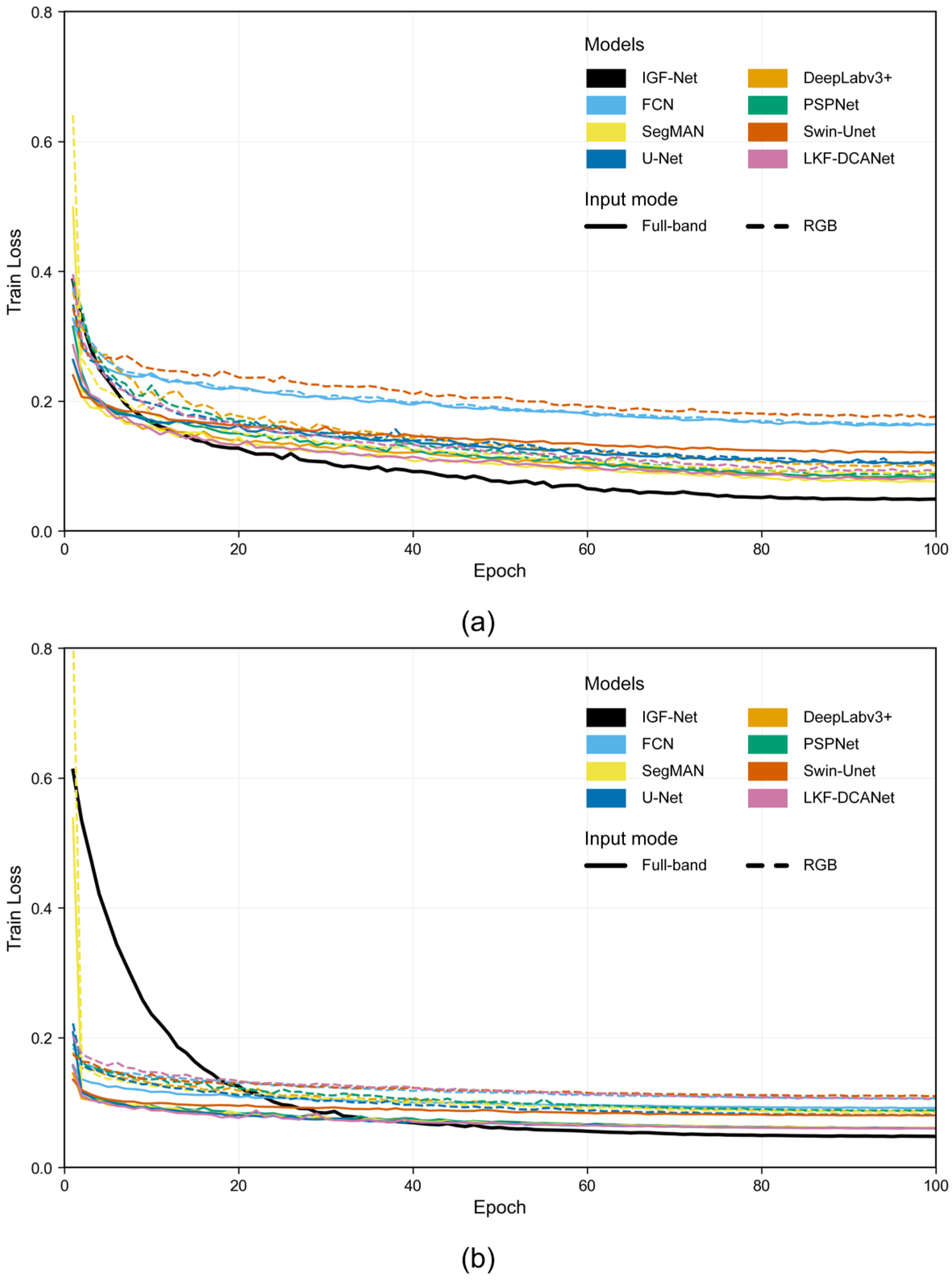
Figure 3 illustrates the training loss curves of the IGF-Net model and its comparative models. From an overall trend perspective, the training loss of all models decreased significantly as the number of training epochs increased, gradually converging to a stable state after approximately 70 epochs, indicating an effective and stable training process. Furthermore, by comparing the loss curves under the two input modes, it can be observed that models trained with the Full-band mode generally exhibited lower loss values in most cases compared to their counterparts using only the RGB mode, and the converged curves showed smaller fluctuations, suggesting a more stable optimization process.

Table 5. Quantitative comparison of different models on TG2-WaterSeg.

Model		Params (M)	FLOPs (G)	FPS	Avg-Time (ms)	Dice	Precision	Recall	IoU
RGB mode $3\times 128\times 128$	DeepLabv3+	40.35	8.68	207.95	4.81	0.8936	0.9103	0.8934	0.8335
	FCN	9.41	7.34	807.11	1.24	0.6668	0.7370	0.6493	0.6086
	PSPNet	48.94	23.51	202.25	4.94	0.8746	0.8928	0.8727	0.8094
	U-Net	31.04	27.37	258.05	3.88	0.8927	0.9204	0.8865	0.8324
	Swin-Unet	27.15	3.85	107.05	9.34	0.8085	0.8765	0.7903	0.7415
	LKF-DCANet	4.30	10.15	334.81	2.99	0.8987	0.9056	0.9056	0.8414
	SegMAN	26.25	15.75	15.38	65.00	0.9021	0.9212	0.8982	0.8445
Full-band mode $14\times 128\times 128$	DeepLabv3+	40.38	8.96	202.52	4.94	0.9096	0.9208	0.9109	0.8542
	FCN	9.41	7.54	806.30	1.24	0.6801	0.7304	0.6691	0.6213
	PSPNet	48.98	23.79	203.62	4.91	0.8891	0.8991	0.8928	0.8281
	U-Net	31.04	27.58	256.77	3.89	0.8941	0.9180	0.8907	0.8388
	Swin-Unet	27.17	3.89	102.23	9.78	0.8834	0.9123	0.8752	0.8237
	LKF-DCANet	4.31	10.25	324.26	3.08	0.9122	0.9223	0.9125	0.8585
	SegMAN	26.25	15.78	15.10	66.22	0.9138	0.9264	0.9123	0.8605
	IGF-Net (ours)	45.15	51.48	97.92	10.21	0.9239	0.9331	0.9235	0.8742

and

Table 6. Quantitative comparison of different models on S2-WaterSeg.

Model		Params (M)	FLOPs (G)	FPS	Avg-Time (ms)	Dice	Precision	Recall	IoU
RGB mode $3\times 256\times 256$	DeepLabv3+	40.35	34.73	160.03	6.25	0.4464	0.6188	0.4031	0.3403
	FCN	9.41	29.35	296.13	3.38	0.1930	0.3492	0.1641	0.1368
	PSPNet	48.94	93.71	90.99	10.99	0.4230	0.5849	0.3782	0.3188
	U-Net	31.04	109.48	89.53	11.17	0.4800	0.6567	0.4320	0.3660
	Swin-Unet	27.15	15.41	73.99	13.51	0.2966	0.5391	0.2456	0.2172
	LKF-DCANet	4.30	40.60	115.37	8.67	0.3079	0.5509	0.2578	0.2270
	SegMAN	26.25	61.78	9.15	109.24	0.4411	0.6316	0.3903	0.3327
Full-band mode $5\times 256\times 256$	DeepLabv3+	40.35	34.93	160.05	6.25	0.6152	0.7225	0.5798	0.4785
	FCN	9.41	29.50	300.05	3.33	0.2484	0.4249	0.2141	0.1735
	PSPNet	48.95	93.92	90.17	11.09	0.5937	0.7063	0.5616	0.4577
	U-Net	31.04	109.63	90.69	11.03	0.6272	0.7395	0.5877	0.4909
	Swin-Unet	27.15	15.44	78.22	12.78	0.5192	0.6977	0.4683	0.3916
	LKF-DCANet	4.30	40.68	115.78	8.64	0.6346	0.7343	0.5949	0.4969
	SegMAN	26.25	61.80	9.11	109.81	0.6236	0.7123	0.5949	0.4855
	IGF-Net (ours)	45.12	205.00	55.87	17.90	0.6370	0.7090	0.6198	0.5009

present the experimental results of IGF-Net and various comparison methods on the TG2-WaterSeg and S2-WaterSeg datasets, respectively, evaluating both model complexity and segmentation performance. It should be noted that due to differences in input sizes between the two datasets and variations in the number of input channels between RGB mode and Full-band mode, the Params and FLOPs of the same model may vary across datasets or input modes. Furthermore, to objectively reflect the model’s performance on the entire test dataset, all reported metrics are averaged over individual test results on every sample in the corresponding test sets.

As shown in Table 5, all models achieve high segmentation accuracy on the TG2-WaterSeg dataset. On this basis, the proposed IGF-Net achieves the best performance, with Dice, Precision, Recall, and IoU reaching 0.9239, 0.9331, 0.9235, and 0.8742, respectively. Compared to the strong baseline SegMAN, IGF-Net improves Dice and IoU by approximately 1.01% and 1.37%, respectively; compared to LKF-DCANet, the improvements are 1.17% and 1.57%. This indicates that even under conditions of high overall accuracy, the proposed method further enhances the overlap between water regions and ground truth, demonstrating superior region modeling and boundary delineation capabilities.

A comparison of the two input modes reveals that most methods perform better in Full-band mode than in RGB mode. For instance, the IoU of DeepLabv3+ increases from 0.8335 (RGB) to 0.8542 (Full-band), U-Net from 0.8324 to 0.8388, and SegMAN from 0.8445 to 0.8605. This suggests that incorporating multispectral bands provides richer spectral discriminative information for the models. In terms of model categories, traditional convolutional networks (e.g., FCN, PSPNet, and U-Net) achieve reasonable results but generally lag behind advanced architectures like LKF-DCANet and SegMAN. This implies that relying solely on local convolutional features or conventional multi-scale aggregation strategies is insufficient to capture fine-grained differences in complex water regions. IGF-Net further outperforms these strong baselines, demonstrating its superior capability in spectral information fusion and water structure representation.

Table 6 presents the experimental results of various models on the S2-WaterSeg. Compared to the results on TG2-WaterSeg (Table 5), all methods exhibit varying degrees of performance decline on S2-WaterSeg. This is attributed to the higher segmentation difficulty of the S2-WaterSeg, characterized by more complex water boundaries, stronger background interference, and more pronounced inter-class confusion. In this more challenging scenario, IGF-Net achieves the highest Dice, Recall, and IoU scores of 0.6370, 0.6198, and 0.5009, respectively, demonstrating its robust water recognition capability in complex remote sensing environments. While LKF-DCANet attains the highest Precision (0.7343), slightly exceeding IGF-Net’s 0.7090, its Recall and IoU remain lower. This indicates that LKF-DCANet’s predictions are more conservative, reducing false positives but increasing false negatives. By contrast, IGF-Net achieves a superior balance between Precision and Recall, resulting in better overall performance on metrics like Dice and IoU.

Regarding input modes, the performance gains of Full-band mode over RGB mode are more pronounced on S2-WaterSeg. For example, DeepLabv3+, PSPNet, U-Net, and LKF-DCANet all show significant improvements in Dice. This highlights that RGB-only information is insufficient for distinguishing water from complex backgrounds, whereas multispectral data provides richer discriminative features. IGF-Net further capitalizes on these advantages, achieving optimal results and underscoring its effectiveness in leveraging multispectral inputs.

From the perspective of model complexity, IGF-Net exhibits higher Params and FLOPs compared to most comparison methods due to its Dual-Branch Feature Encoder Module. Specifically, on TG2-WaterSeg and S2-WaterSeg, IGF-Net’s Params are 45.15 M and 45.12 M, respectively, with FLOPs of 51.48 G and 205.00 G. In terms of inference efficiency, it achieves FPS values of 97.92 and 55.87 on the two datasets, corresponding to Avg-Time of 10.21 ms and 17.90 ms. The reduced inference speed on S2-WaterSeg is primarily attributed to the increased computational overhead caused by higher spatial resolution in input images. Overall, while IGF-Net is not the fastest model, it maintains acceptable practical operational efficiency.

A comprehensive analysis of complexity and performance demonstrates that IGF-Net achieves significant accuracy improvements despite its increased model scale and computational cost. Although its inference efficiency lags behind lightweight models, it outperforms all others in key metrics such as Dice and IoU. This indicates that IGF-Net effectively trades moderate computational overhead for superior segmentation performance. For remote sensing water body segmentation tasks prioritizing high-precision extraction, this accuracy-efficiency trade-off is justified and practically valuable. Compared to pursuing extreme inference speed, achieving higher regional overlap accuracy and more complete water body identification is typically more critical in such applications.

4.2.3. Qualitative Comparison Results and Discussion

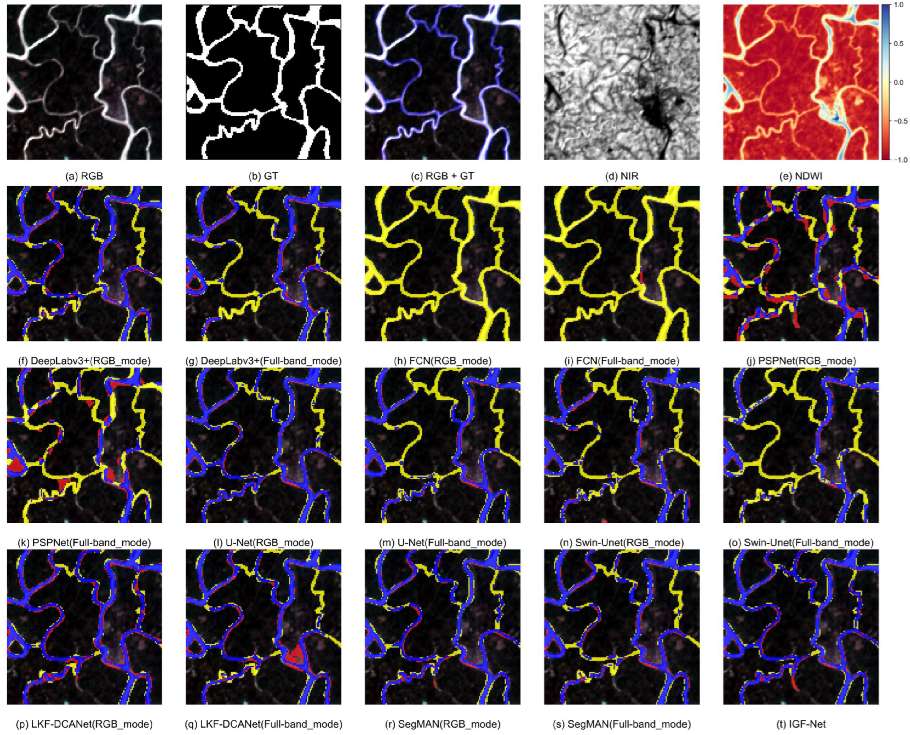
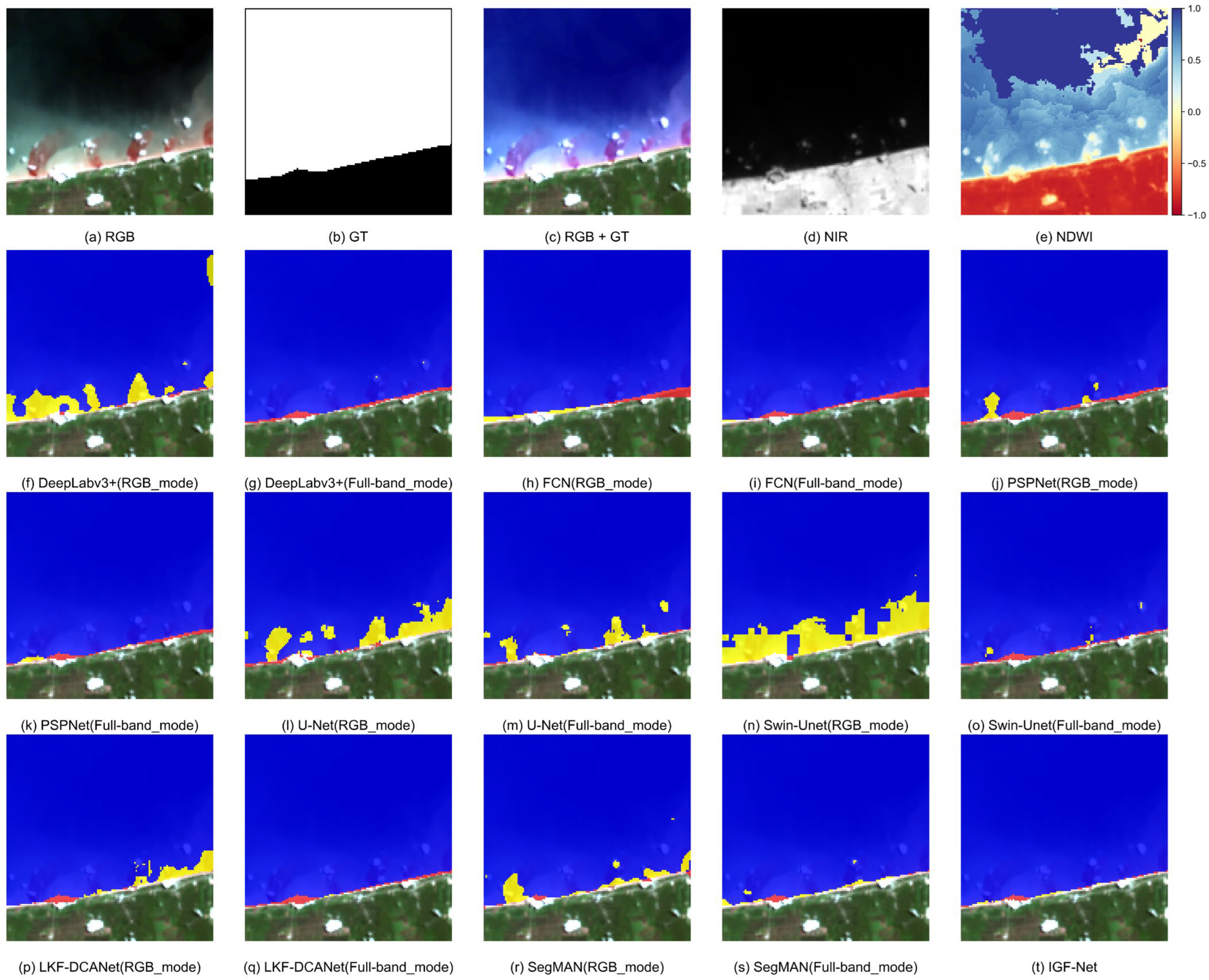
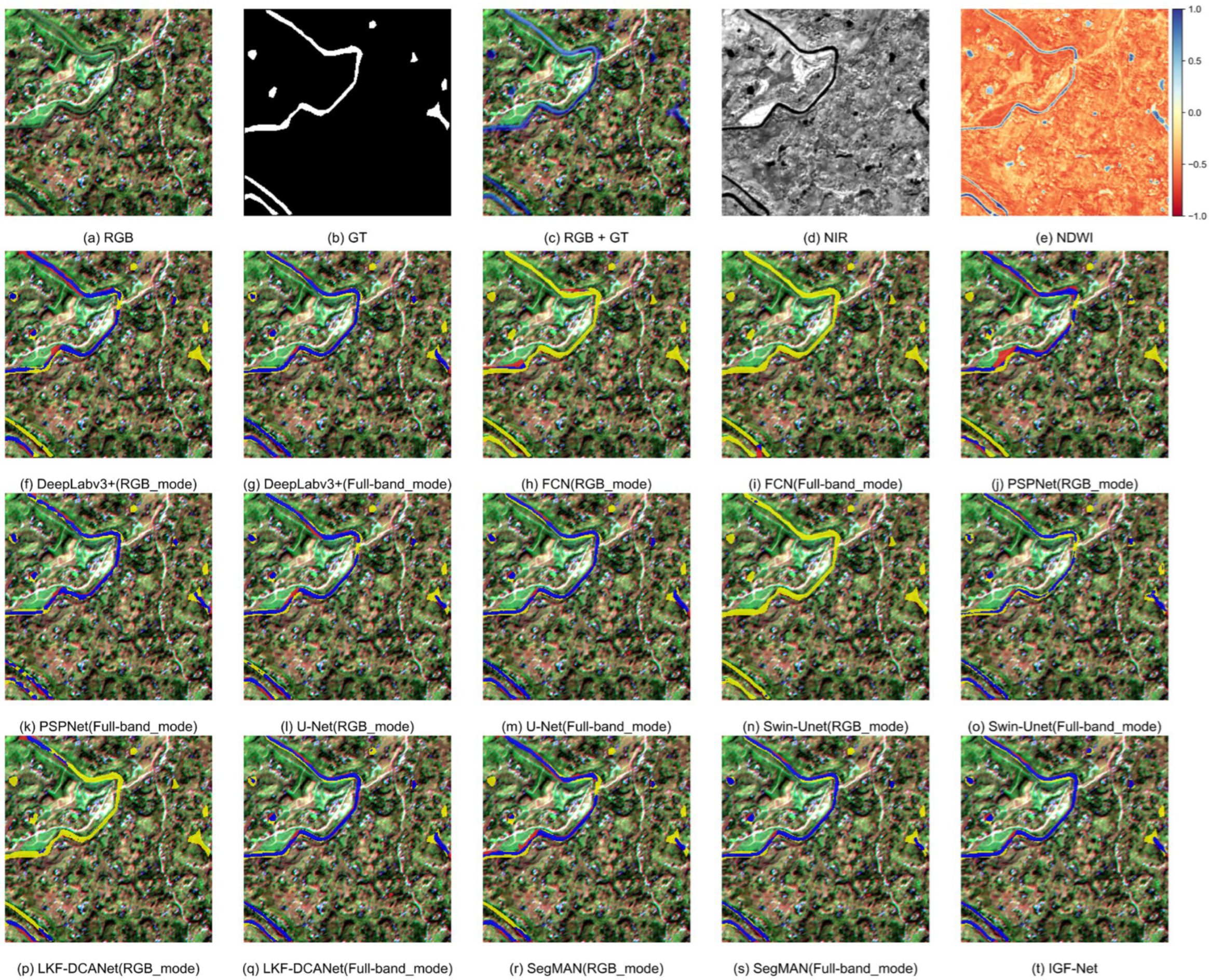
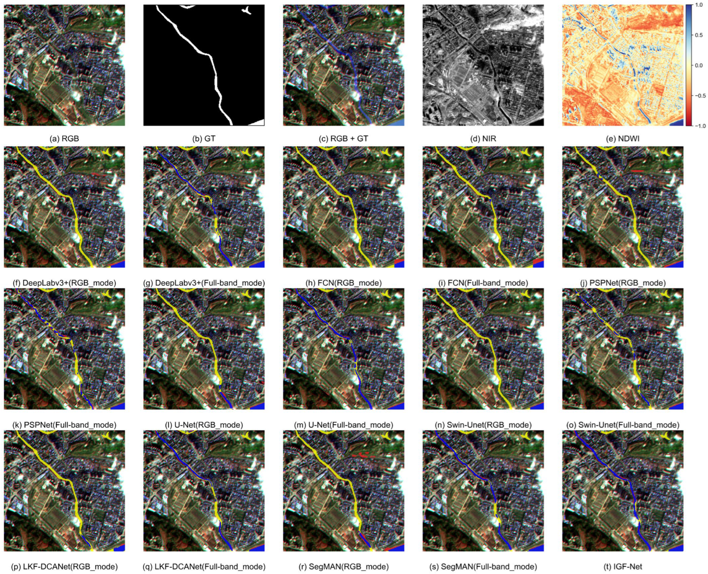
To enable direct visual comparison of model performance, this subsection presents visualizations of prediction results and associated errors generated by IGF-Net and comparative models across four typical scenarios in the TG2-WaterSeg and S2-WaterSeg (Figure 4, Figure 5, Figure 6 and Figure 7). Each figure incorporates multi-modal reference images: (a) input RGB image providing spatial context; (b) binary ground truth water mask where white denotes water regions and black indicates background; (c) RGB image overlaid with semi-transparent blue water masks to clarify segmentation objectives; (d) water-sensitive near-infrared band grayscale image highlighting reflective characteristics; (e) NDWI map computed through conventional spectral index calculations serving as baseline reference. Standardized error maps in subfigures (f–t) of each figure (Figure 4, Figure 5, Figure 6 and Figure 7) facilitate comparison of the segmentation results across all models, using blue, red, and yellow hues to denote true positives, false positives, and false negatives, respectively.

As shown in Figure 4, this sample is selected from the TG2-WaterSeg test set. It exhibits distribution characteristics of a narrow, continuous, and multi-branch water system, presenting a densely meandering spatial morphology. This configuration imposes high demands on the model’s capabilities for fine-grained structure perception, boundary localization, and topological connectivity preservation. The comparison results in Figure 4f–s reveal consistent failure modes across different methods in this complex scenario. In RGB mode, most methods demonstrate varying degrees of omission and connectivity disruption in two critical areas: the upper multi-branch confluence region and the mid-lower zigzag narrow tributaries. These errors manifest as fragmented river segments, incomplete branch connections, and disappearance of terminal tributaries. When switching to Full-band mode, the incorporation of additional multispectral band information effectively reduces omissions in main channels. Most methods show improved response integrity for the right main channel and upper branches compared to RGB mode, validating the discriminative value of supplementary spectral bands for water body identification. However, even with Full-band mode, comparative methods still exhibit notable limitations: (1) persistent local discontinuities or connection errors in mid-lower narrow tributaries and bifurcation nodes; (2) trade-offs between reduced omissions and new artifacts, including boundary misalignment, local morphological distortion, or river width estimation errors. These issues are especially pronounced in highly sinuous reaches and terminal narrow tributaries. In contrast, the IGF-Net result in Figure 4t demonstrates superior structural restoration capability. Its predictions not only achieve more complete tracking of the right longitudinal main channel but also better preserve: (1) the connectivity of upper multi-branch systems, (2) the continuous extension of mid-lower zigzag tributaries, and (3) tighter boundary alignment with ground truth contours at sharp bends and confluence nodes. Overall, IGF-Net surpasses other methods in three key aspects: narrow channel preservation, branch topology restoration, and complex boundary fitting. This performance underscores its enhanced fine-grained structural preservation capability in complex water network environments.

Figure 5 presents a comparative visualization of segmentation results from multiple methods applied to a typical coastal scene in the TG2-WaterSeg. This sample exhibits characteristic features of the land-water interface, with the coastline demonstrating a diagonal trajectory from the lower-left to upper-right. The upper region contains continuous open water, while the lower area comprises a narrow land strip. The land-water boundary is characterized by both considerable length and subtle local undulations. Analysis of Figure 5a,d reveals that nearshore shallow water and intertidal zones lack ideal uniform spectral responses, instead displaying pronounced grayscale gradients and textural disturbances. This scenario necessitates that models not only demonstrate robust water body identification but also effectively address challenges including boundary localization accuracy, transitional zone discrimination, and local noise suppression. Comparative analysis of prediction results in Figure 5f–s identifies two predominant error patterns among baseline methods. The first involves systematic deviations along the true shoreline, manifesting as boundary false positives/negatives relative to ground truth annotations—a consistent observation across most methods indicating generalized coastline localization errors. The second error type appears as contiguous misclassified patches within the nearshore transition zone, where certain models generate extensive blocked errors particularly adjacent to high-reflectance interference areas. Notably, these phenomena exhibit mode-dependent variations: RGB mode shows exacerbated coastline misalignment and speckle artifacts, whereas Full-band mode leverages additional multispectral information to improve main-body segmentation. While full-band inputs reduce overall error magnitude compared to RGB mode, persistent irregularities remain in shoreline details. This suggests that although multi-spectral data enhances general separability, it fails to resolve fundamental challenges in precise coastal boundary alignment. Conversely, IGF-Net demonstrates superior shoreline reconstruction capability. As evidenced in Figure 5t, its errors are constrained to an immediately adjacent narrow band along the true shoreline. The model significantly suppresses large-area patch errors in shallow waters while minimizing discrete noise responses. Particularly noteworthy is the high boundary consistency achieved in both mid-section and terminal right segments of the coastline. These results verify IGF-Net’s dual capability of accurately distinguishing main water bodies from land masses while maintaining precise boundary localization within complex transition zones.

Figure 6 presents a typical mountainous sample from the S2-WaterSeg, containing a meandering narrow main channel, a partially truncated river segment in the lower-left, and several discrete small water bodies distributed across the upper-middle, upper-right, and left-middle regions. The scene exhibits strong terrain-induced texture interference, pronounced curvature variations in the central bend of the main channel, and diminutive spatial extent of isolated water bodies, requiring models to preserve channel continuity while maintaining sensitivity to minuscule targets. Comparative analysis of Figure 6f–s reveals systematic error patterns among baseline methods, predominantly in two domains: high-curvature narrow sections of the main channel and discretely positioned small water bodies. Under RGB modality, several methods exhibit width shrinkage and local discontinuities within the central bend and narrow reaches. For isolated water bodies, multiple models generate fragmented responses confined to central regions while failing to reconstruct complete boundaries, occasionally resulting in total omission. Full-band implementations improve main-channel continuity, particularly in the central bend and lower-left segment, confirming that supplementary spectral information enhances water-background separability. However, for small water bodies covering minimal pixels, numerous comparative methods still demonstrate boundary contraction artifacts, capturing core regions while failing to recover full spatial extent. Conversely, IGF-Net achieves complete recovery of the tortuous main channel while maintaining geometric fidelity at the highly contorted central bend. It consistently detects all small water bodies without global omission failures. Although minor under-segmentation persists at boundaries of extremely small targets, such errors remain strictly peripheral without compromising core region recovery. This demonstrates IGF-Net’s superior robustness in handling size-variant water feature extraction under complex mountainous conditions.

Figure 7 shows a representative urban scene from the S2-WaterSeg dataset. The target water body is dominated by a narrow main channel extending diagonally from the upper to the lower part of the image, with slight width variations and bends in the densely built central region. Several tiny isolated water bodies are also present near the upper-right and upper boundary. The scene is highly challenging because abundant buildings, roads, and other artificial structures introduce dense background textures, while linear roads, building edges, bright objects, and shadows produce strong spatial and spectral confusion with the narrow channel. As shown in Figure 7f–s, most baseline methods under RGB mode only respond to the upper and lower segments of the main channel, while the central urban section is frequently missing or severely fragmented, accompanied by width shrinkage and boundary misalignment. Full-band inputs improve channel recognition and allow longer continuous segments to be recovered, but many methods still suffer from discontinuities, boundary drift, and inaccurate width estimation in the narrow central section and other complex urban areas. These results indicate that enhanced spectral information improves separability but remains insufficient for preserving elongated water structures in urban environments. In contrast, IGF-Net achieves complete and continuous extraction of the main channel across the image center, with substantially better alignment to the ground truth in densely built and highly disturbed regions. Although slight omissions remain for tiny isolated water bodies near the upper boundary, IGF-Net shows clear advantages in main-channel integrity, boundary stability, and overall structural consistency.

4.2.4. Cross-Temporal Migration Experiment and Result Analysis

To systematically evaluate the model’s generalization capability and prediction stability under temporal variations, this study conducts cross-temporal migration experiments using the temporally extended S2-WaterSeg. Unlike the “training-testing” paradigm within the same temporal phase, cross-temporal validation better aligns with real-world scenarios where models must process multi-temporal remote sensing observations. In practice, models often encounter images acquired at different times, where factors such as solar elevation angle, atmospheric conditions, sensor status, and seasonal surface changes introduce significant variations in spectral response, brightness distribution, textural features, and background context. Such temporal shifts induce distribution discrepancies that increase the difficulty of object identification and segmentation. Due to the lack of pixel-level annotations for the newly added temporal data, unified quantitative metrics cannot rigorously evaluate model performance on unseen phases. Therefore, this study adopts a qualitative analysis: the IGF-Net model trained on the original phase (April 2018) is directly applied to two unseen phases (December 2018 and February 2019) for inference. Prediction results are then compared and analyzed alongside NDWI data for two representative samples.

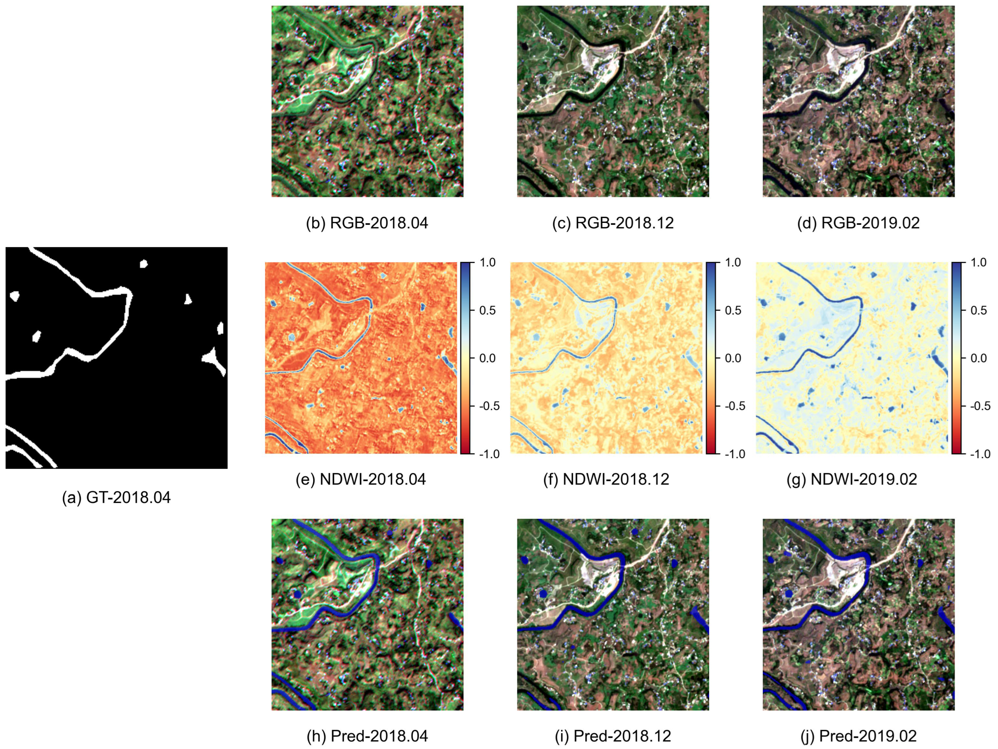
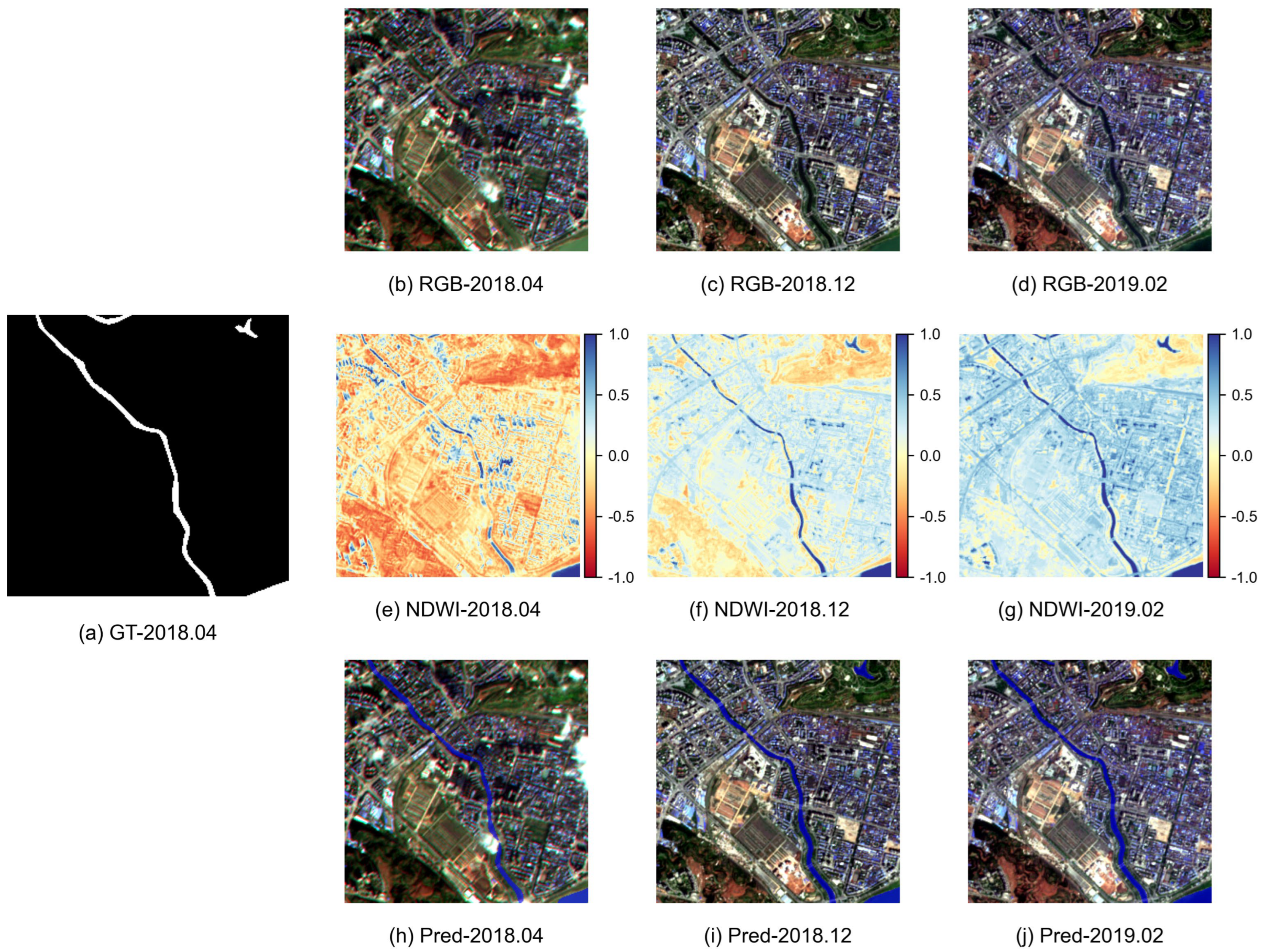
Figure 8 and Figure 9 illustrate representative examples from the cross-temporal migration experiment. Panel (a) displays the ground truth annotation for the training phase (April 2018). Panels (b)–(d) show RGB images acquired in April 2018, December 2018, and February 2019, respectively. Panels (e)–(g) present the corresponding NDWI results for these phases. Finally, panels (h)–(j) depict prediction overlays generated by the model trained on the April 2018 phase and applied to all three temporal phases.

As shown in Figure 8, this sample exhibits pronounced observational differences across the three temporal phases. Compared to April 2018, the RGB images from December 2018 and February 2019 display notable changes in overall color tone, brightness gradients, and background textural patterns, indicating that temporal variations have induced a shift in the input feature distribution. For water regions, the main river channel retains its spatial positioning and overall trajectory across all three phases, with visual discrepancies primarily observed in localized shorelines, near-shore transitional areas, and the morphology of scattered small water bodies. The corresponding NDWI results further highlight that while the main channel sustains consistently high spectral responses across different acquisition dates, the index values over non-water backgrounds exhibit distinct alterations. Despite these input variations, the model trained on April 2018 data, when applied to the two unseen phases, successfully maintains continuous extraction of the main river channel. It preserves connectivity and curvilinear morphology effectively, with only minor adaptations at local boundaries and small-scale water features. This underscores the model’s robust ability to retain dominant water structures and deliver stable predictions despite temporal shifts, demonstrating strong cross-temporal generalization.

As illustrated in Figure 9, this sample demonstrates significant visual discrepancies across the three temporal phases. Notably, the April 2018 image appears overall darker with distinct bright spots, contrasting sharply with December 2018 and February 2019 in both imaging aesthetics and textural sharpness. This highlights that cross-temporal model migration must address not only seasonal shifts but also perturbations arising from variable imaging conditions. Furthermore, NDWI analysis confirms that while the main river channel retains strong spectral responses across all dates, the index values over non-water backgrounds show pronounced alterations. Specifically, background regions in December 2018 and February 2019 exhibit systematically higher NDWI values compared to April 2018, exacerbating land-water ambiguity risks in urban settings. Despite these challenges, the primary river skeleton remains spatially consistent across phases, maintaining identical positional alignment and directional trends, with minor deviations confined to narrow channels, bends, and vicinities of small tributary water bodies. The model robustly sustains the main channel’s connectivity throughout all phases. However, in April 2018, cloud cover and shadowing in the upper-right quadrant of the input image caused partial misdetection of small water features, whereas these areas were accurately resolved in later phases. This resilience underscores the model’s capacity to generalize across temporal variability.

4.3. Ablation Study: Replacing the Fusion Module

4.3.1. Ablation Experiment Setup

To systematically evaluate the contribution of the proposed IGFM to water-body semantic segmentation in remote sensing images, this study designs a corresponding ablation experiment: On the IGF-Net architecture, the impact mechanism of sequentially replacing or removing the fusion module on multi-source feature fusion (the visual branch and the spectral branch) is analyzed from both quantitative metrics and interpretability visualization perspectives. To ensure comparability among different model variants and conclusion reliability, all experiments follow consistent parameter settings, with differences limited solely to the model fusion method.

Specific experimental models are as follows:

Model 1: The baseline control model. This model completely removes the IGFM and uses only simple channel concatenation followed by a 1 × 1 convolution for feature fusion and dimensionality reduction. It is designed to examine whether direct feature concatenation and convolutional operations are sufficient for multi-source fusion tasks without explicit interaction/attention mechanisms.

Model 2: Replaces the IGFM with an iterative attention feature fusion module [35]. This module progressively refines fused features through cascaded/iterative attention while enhancing local salient regions. This configuration allows for a direct comparison between the IGFM and an iterative-optimization-based attention fusion approach.

Model 3: Replaces the IGFM with a bilinear attention fusion module [36]. This module captures high-order correlations between features through bilinear interaction modeling to obtain finer-grained interactive representations. It is used to evaluate the applicability of high-order feature interaction in multispectral water-body segmentation and to compare the module’s interaction modeling approach with that of the IGFM.

Model 4: Replaces the IGFM with a cross-modal attention feature fusion module [37]. This module has demonstrated strong mutual-information extraction capability in multimodal data fusion. In this experiment, it is introduced into the multispectral remote-sensing scenario to examine the module’s effectiveness in handling two types of feature sources: spectral and spatial.

Model 5: Replaces the IGFM with a dual cross-attention mechanism module [38]. This module enables mutual enhancement of the two branch features through two-stage, bidirectional attention interaction, providing strong semantic-level representation capacity. It is thus employed to benchmark the performance of the IGFM against an advanced cross-attention architecture.

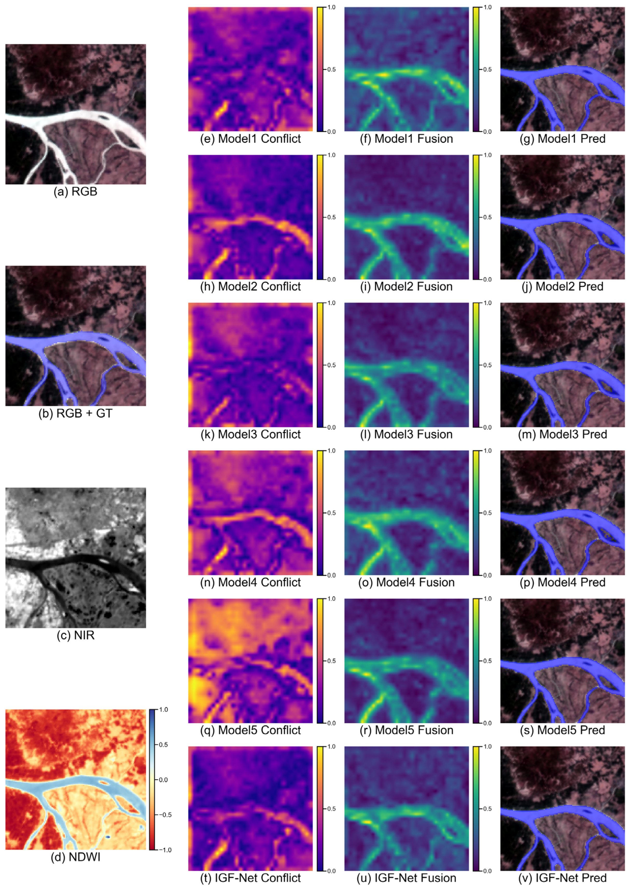
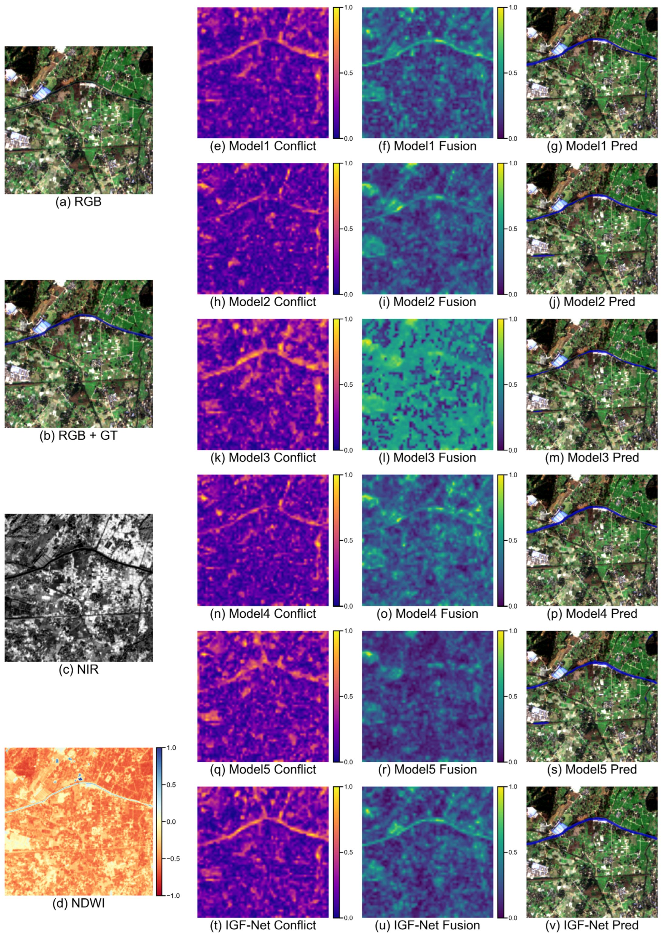
As discussed in Section 3.2, the Dual-Branch Feature Encoder Module exhibits fundamental differences in feature representation: the visual branch primarily carries general spatial-semantic knowledge acquired through transfer learning, while the spectral branch focuses on subtle reflectance variations corresponding to different land classes in non-RGB bands of multispectral data. To systematically investigate the internal working mechanisms of different fusion modules during the “visual-spectral” feature integration process, this study computes and visualizes feature conflict maps at the input end and post-fusion feature activation maps at the output end of the fusion modules, thereby revealing their intrinsic fusion mechanisms.

Specifically, given the two pre-fusion branch features, $F_{\mathrm{v}}$ and $F_{\mathrm{s}}$, this paper first calculates the $L_2 \mathrm{norm}$ of the feature vector at each spatial position as the response intensity for that position, thereby obtaining the response intensity maps for both branches:

$$\begin{array}{l}{M}_{\mathrm{v}}(x,y)=‖F_{\mathrm{v}}{(:,x,y)‖}_2\\ M_{\mathrm{s}}(x,y)=‖F_{\mathrm{s}}{(:,x,y)‖}_2\end{array}$$

(11)

On this basis, the absolute difference in response intensity between the two branches is defined as the raw conflict intensity $D_{\mathrm{raw}}$.

$$D_{\mathrm{raw}}(x,y)=\left|M_{\mathrm{v}}(x,y)\right.\left.-M_{\mathrm{s}}(x,y)\right|$$

(12)

To visualize the spatial distribution of feature conflicts, the raw conflict intensity $D_{\mathrm{raw}}(x,y)$ is further normalized into the range [0, 1] using a min–max normalization strategy. Specifically, for each sample, the minimum and maximum values of the conflict map are computed, and the normalized conflict intensity is defined as:

$$D_{\mathrm{norm}}(x,y)={\displaystyle \frac{D_{\mathrm{raw}}(x,y)-D_{\min }}{D_{\max }-D_{\min }+\mathsf{\epsilon }}}$$

(13)

where $D_{\min }$ and $D_{\max }$ denote the minimum and maximum values of the raw conflict map for the current sample, respectively, and $\mathsf{\epsilon }$ is a small positive constant to avoid division by zero. This normalization rescales the conflict intensity of each sample to the interval [0, 1], facilitating clearer visualization of spatial conflict patterns.

The post-fusion feature activation map is defined as the spatial response obtained by applying the $L_2 \mathrm{norm}$ along the channel dimension to the fused feature tensor $T$ output by the fusion module:

$$A(x,y)={‖T(:,x,y)‖}_2$$

(14)

Then, min-max normalization is applied to $A(x,y)$ to map it into the range [0, 1]:

$$A_{\mathrm{norm}}(x,y)={\displaystyle \frac{A(x,y)-A_{\min }}{A_{\max }-A_{\min }+\mathsf{\epsilon }}}$$

(15)

Due to the use of sample-specific min-max normalization, the pixel values in the conflict map and post-fusion feature activation map represent relative differences between spatial locations rather than absolute quantities comparable across samples. The performance of the fusion module can be evaluated from two dimensions: first, the spatial concentration of boundary activations—whether high activations are localized in water-land transition zones; second, the quality of activation suppression in non-boundary regions—whether feature energy within water bodies and backgrounds is effectively suppressed. Furthermore, since both maps are generated by upsampling low-resolution features, the interpolation process tends to blur fine-grained structures and introduce visible diffusion artifacts in corresponding areas. Therefore, these maps are more suitable for observing overall distribution patterns and their correlation with error-prone regions, rather than serving as precise pixel-level boundary references.

4.3.2. Quantitative Ablation Results

Module-replacement experiments were conducted on TG2-WaterSeg and S2-WaterSeg.

Table 7. Quantitative Results of Module-Replacement Experiments on TG2-WaterSeg and S2-WaterSeg.

Models		IoU	Dice	Precision	Recall
TG2-WaterSeg	Model 1	0.8712	0.9224	0.9269	0.9287
	Model 2	0.8713	0.9227	0.9271	0.9284
	Model 3	0.8674	0.9207	0.9339	0.9166
	Model 4	0.8734	0.9239	0.9221	0.9367
	Model 5	0.8686	0.9210	0.9336	0.9184
	IGF-Net (ours)	0.8742	0.9239	0.9331	0.9235
S2-WaterSeg	Model 1	0.4918	0.6283	0.7194	0.6024
	Model 2	0.4893	0.6263	0.7158	0.5957
	Model 3	0.4774	0.6145	0.7036	0.5926
	Model 4	0.4971	0.6322	0.7006	0.6154
	Model 5	0.4601	0.5946	0.6914	0.5740
	IGF-Net (ours)	0.5009	0.6370	0.7090	0.6198

summarizes the quantitative results of each substitution scheme on the respective test sets, with the main network structure and training configuration held identical. In these experiments, IGF-Net serves as the baseline for the replacement experiments, and its results are consistent with those reported in the earlier comparative experiments.

Overall, IGF-Net achieves relatively strong comprehensive performance on both datasets, which verifies the effectiveness of the IGFM for feature fusion. In particular, on the more challenging S2-WaterSeg dataset, IGF-Net obtains the best results in IoU, Dice, and Recall, indicating that the IGFM may be more conducive to coordinating the complementary information between the visual branch and the spectral branch under complex backgrounds and diverse water-body morphologies.

On TG2-WaterSeg, all models perform well overall, with IoU values above 0.8670 and Dice values above 0.9200. IGF-Net achieves the highest IoU (0.8742) and the joint-highest Dice (0.9239) on this dataset, demonstrating the potential to further improve the overall overlap between predictions and ground-truth annotations. Compared with IGF-Net, Model 1 yields slightly lower results, suggesting that although simple concatenation and linear compression can preserve a certain amount of complementary information, they may still be insufficient in terms of explicit interaction modeling and feature selection. Model 2 brings only marginal performance changes, indicating that iterative attention is more oriented toward enhancing local salient regions, while its effect on modeling semantic consistency between features from different sources is relatively limited. Model 3 achieves the highest Precision of 0.9339, which to some extent indicates that bilinear high-order interaction helps enhance category discriminability and reduce false positives. However, its Recall decreases to 0.9166, suggesting that this method may adopt a relatively conservative prediction strategy, resulting in insufficient coverage of some real water-body regions and ultimately causing its IoU and Dice to be slightly lower than those of IGF-Net. Among all replacement schemes, Model 4 performs most closely to IGF-Net: its Dice is equal to that of IGF-Net, and its Recall reaches the highest value of 0.9367. This indicates that cross-modal attention has certain advantages in mining the complementary relationship between visual features and spectral features and in improving target coverage. However, its relatively lower Precision suggests that while expanding the target response range, this method may also introduce more false detections. Model 5 still exhibits a trend of relatively high Precision but comparatively low Recall, which to some extent indicates that although dual cross-attention strengthens the semantic correlation between branches, it has not yet achieved a more desirable balance between complete target-region recovery and false-positive control. Overall, IGFM shows better comprehensive stability on TG2-WaterSeg.

On S2-WaterSeg, the performance advantage of IGF-Net is more significant. Its IoU, Dice, and Recall reach 0.5009, 0.6370, and 0.6198, respectively, outperforming all alternative models on these three metrics. Specifically, although Model 1 achieves the highest Precision (0.7194), its IoU and Dice are both lower than those of IGF-Net. This suggests that simple fusion methods are prone to missed detections in complex water-body regions. From the experimental results, Model 2 does not show a more obvious performance advantage over Model 1, which to some extent indicates that the effectiveness of the iterative attention strategy in this complex scenario is not particularly prominent. The overall performance of Model 3 declines, which may suggest that although bilinear high-order interaction can enhance correlation modeling between features, it is also more likely to introduce noise interference under complex background conditions, thereby affecting the stability of the fusion results. Model 4 remains highly competitive, with its IoU, Dice, and Recall ranking only behind IGF-Net, indicating that the cross-modal interaction mechanism has strong application potential in multi-source feature fusion. Compared with Model 4, IGF-Net achieves slight improvements on all metrics, suggesting that the IGFM not only constructs effective cross-branch semantic associations, but also achieves a better balance between redundant-information suppression and effective-feature preservation. In contrast, Model 5 does not show obvious overall advantages on this dataset, which may indicate that although its bidirectional cross-coupling mechanism enhances semantic interaction between the two branches, its improvement in information propagation stability and error control remains relatively limited in the current task scenario.

4.3.3. Qualitative Ablation Results and Discussion

For a visual demonstration of the differences among fusion modules, this section presents two representative samples from the TG2-WaterSeg and S2-WaterSeg test sets. Each image follows a consistent layout: the left column sequentially shows the RGB image, the RGB image with ground truth overlay, the NIR image, and the NDWI image; the right column displays the predictions of benchmark models and IGF-Net, along with their corresponding conflict and fusion maps. Notably, because all models are trained end-to-end, each fusion strategy indirectly shapes the learning of branch features via backpropagation. As a result, distinct conflict patterns emerge even during feature extraction, ultimately affecting the final fusion outcomes. Hence, conflict and fusion maps are best interpreted as references for understanding feature abstraction, rather than as absolute evidence of model performance.

As illustrated in Figure 10, this case study presents a riverine scene from the TG2-WaterSeg dataset. The region exhibits heterogeneous land-cover composition, including riverine water bodies, exposed soil, and vegetated areas. The water network shows a characteristic meandering morphology, with narrow tributary bifurcations in the lower section and shallow shoals along the right bank. Such geomorphological complexity introduces pronounced class ambiguity and spatial uncertainty at the land–water transition zones.

In the conflict maps, all models produce high-magnitude responses along the boundaries of the narrow tributaries in the lower part of the image, indicating that these regions—characterized by slender water morphology and weak textural contrast with the surrounding background—constitute highly uncertain boundaries. Model 2, Model 4, and IGF-Net form relatively continuous conflict-response bands along the boundaries of the main river channel, whereas Model 1 and Model 3 exhibit weaker conflict responses near the main river trunk. In contrast, Model 5 produces extensive patch-like high responses over land areas, reflecting significant discrepancies in the Dual-Branch Feature Encoder Module when representing background land features. Overall, several comparative methods still retain varying degrees of background conflict residuals. By contrast, IGF-Net concentrates high-conflict responses primarily along genuine land–water boundaries and key structural details while suppressing non-boundary regions to low-value backgrounds. This demonstrates IGF-Net’s stronger capability in conflict localization and noise suppression.

In the fusion activation maps, although all models produce activations along land–water transition zones, clear differences emerge in spatial morphology and background suppression. At the narrow downstream tributaries, IGF-Net’s activations adhere more closely to the boundaries, forming sharper high-activation zones than those of the comparative models and thereby achieving better edge definition and diffusion-noise suppression. In internally inconsistent water regions such as the right-bank shoal, IGF-Net generates more concentrated activation patterns, enabling more precise delineation of local boundary details during post-processing.

In the final segmentation results, all methods successfully reconstruct the macroscopic contour of the main river channel, demonstrating robust large-scale water-body recognition capability. However, inter-model differences become evident in uncertain regions such as narrow tributaries and shoal vicinities, mainly manifested as pixel-level boundary deviations and contour discontinuities. Benefiting from accurate conflict localization and low-redundancy fusion representations with enhanced background discrimination, IGF-Net achieves the best performance on this sample, reaching an IoU of 0.8667 compared with 0.8644 (Model 1), 0.8496 (Model 2), 0.8465 (Model 3), 0.8449 (Model 4), and 0.8592 (Model 5). Although these improvements are only subtly visible in thumbnail visualizations, the quantitative metrics confirm IGF-Net’s consistent advantages in handling complex boundaries and fine-grained details.

As illustrated in Figure 11, this S2-WaterSeg scene depicts a rural agricultural canal landscape. The main channel arcs across the upper part of the image with a slender, elongated morphology. Surrounding farmland is fragmented into small parcels and interwoven with dense linear structures such as paths and field ridges. These elements create strong spectral and morphological similarities between narrow water bodies and the background, substantially increasing the difficulty of land–water boundary discrimination.

The conflict maps show strong responses around the main channel for all models, confirming this region as the primary locus of cross-modal representation discrepancies. However, their spatial distributions differ markedly. Model 1 roughly outlines the channel conflict zone but retains noticeable background noise. Model 2 and Model 4 exhibit more dispersed point-like and strip-like patterns across the scene, including redundant conflicts in non-water areas. Model 3 and Model 5 present patchy and discrete high responses. In contrast, IGF-Net produces high-conflict responses that closely follow the true course and boundaries of the channel, demonstrating more accurate conflict localization.

In the fusion activation maps, all models except Model 3 and Model 5 generate responses along the land–water transition zones. Although Model 1, Model 2, and Model 4 cover the channel area, residual moderate background responses may still cause misclassification. Model 3 produces large, spatially unselective patch-like activations with blurred boundaries, while Model 5 shows generally weak activations accompanied by scattered spurious responses. By comparison, IGF-Net maintains continuous and concentrated activations along the main channel with cleaner background suppression, enabling more reliable discrimination of slender water bodies under complex textures.

The final segmentation results show that all methods recover the overall course of the channel, but two typical failure modes remain: linear infrastructures such as field ridges and paths often induce local false detections, and narrow channel segments may exhibit discontinuities or inaccurate width estimation. Benefiting from more accurate conflict localization and low-redundancy fusion representations, IGF-Net achieves the best performance on this sample, reaching an IoU of 0.6627. This surpasses Model 1–5 (0.6200, 0.6021, 0.4917, 0.5252, and 0.5159, respectively), representing a 4.27-percentage-point improvement over the strongest competing method (Model 1). These results further validate the effectiveness of the IGFM in complex backgrounds with slender water bodies.

5. Discussion

The experimental results presented in Chapter 4 demonstrate that IGF-Net achieves superior performance on both TG2-WaterSeg and S2-WaterSeg. Its core module, IGFM, explicitly models modality-specific differences and modality-consistent activations, enabling adaptive fusion of visual and spectral features.

On TG2-WaterSeg, where most models already exhibit competitive performance indicating saturation, IGF-Net still achieves meaningful improvements in key metrics. Notably, IoU reaches 0.8742—a gain of 1.4 percentage points over the best baseline. This gain under saturated conditions validates IGF-Net’s effectiveness in detail preservation and boundary optimization. On the more challenging S2-WaterSeg, IGF-Net shows even greater quantitative improvements, suggesting IGFM’s advantages become more prominent with increased task complexity. Qualitative analyses reveal IGF-Net better preserves fine-grained structures like narrow tributaries and small isolated water bodies compared to other methods. Cross-temporal experiments demonstrate robustness against seasonal variations and imaging condition changes, maintaining main channel continuity through structural/contextual feature learning rather than shallow spectral cues.

However, IGF-Net’s dual-branch feature encoder module introduces higher computational costs: on TG2-WaterSeg, it requires 45.15 M parameters, 51.48 G FLOPs, and achieves 97.92 FPS, showing lower efficiency than lightweight methods. This impacts deployability in resource-constrained scenarios. Additionally, the model lacks systematic validation under extreme atmospheric conditions or with auxiliary data (e.g., DEM and SAR). Ablation studies show while IGFM achieves balanced metric performance, scenario-specific optimization remains necessary for precision/recall requirements.

Despite these limitations, IGF-Net’s accurate water extraction under complex conditions holds significant practical value. High IoU/Dice scores translate to reliable land cover products for flood monitoring, water resource management, and environmental change detection. The structure-preserving capability is particularly crucial for monitoring narrow channels, coastal erosion, and small urban/agricultural water bodies where errors impact downstream analyses. Furthermore, IGFM can be extended to other remote sensing tasks that require multispectral or multi-source data fusion.

6. Conclusions

This study addresses the challenges of pre-trained model transferability and inadequate multi-band feature fusion in water body segmentation for multispectral remote sensing images, proposing a novel segmentation network and constructing a supporting dataset. The main contributions and conclusions are as follows:

(1)

The Tiangong-2 Remote Sensing Image Water Body Semantic Segmentation Dataset was constructed and made publicly available. This dataset provides 3776 multispectral image groups with pixel-level fine annotations for water body segmentation. To systematically validate model generalization, the public Sentinel-2 Water Segmentation Dataset was also introduced, enabling comprehensive performance evaluation across different sensors, band combinations, and scene complexities.

(2)

This study proposes the IGF-Net architecture to address the challenges of poor transferability in pre-trained models and inadequate multi-source feature fusion. The network employs a dual-branch encoder as its backbone, centered around the IGFM. Through a cascaded mechanism integrating difference-co-occurrence parallel modeling, channel-context prior, and adaptive temperature control, this module achieves adaptive deep fusion of visual and spectral features. This design not only promotes training stability but also improves water body segmentation accuracy.

(3)

Extensive experiments validate the effectiveness and generalization capability of IGF-Net and its core module, IGFM. On TG2-WaterSeg, IGF-Net achieves highly competitive performance (IoU 0.8742), demonstrating its ability to further refine segmentation details in scenarios with relatively limited room for improvement. On the more challenging S2-WaterSeg, IGF-Net shows clearer advantages in key metrics such as IoU (0.5009) and Dice (0.6370), indicating that IGFM is more effective at coordinating complementary information from the visual and spectral branches and achieves a better balance between segmentation completeness and false-positive suppression. Ablation studies comparing five alternative fusion modules further confirm that IGFM provides stronger overall stability, particularly in complex scenarios. Visualization results further show that IGF-Net concentrates cross-modal discrepancies on true boundaries and critical structural regions while suppressing background interference, producing more continuous and clearer responses to complex boundaries and elongated water bodies. Cross-temporal experiments demonstrate that IGF-Net maintains the continuity of major channels despite seasonal variations and imaging condition differences, indicating its ability to learn relatively robust features based on structural and contextual cues.

(4)

Complexity analysis reveals that IGF-Net’s dual-branch design leads to higher computational costs compared to lightweight methods, which may limit deployment in resource-constrained scenarios. The model has not been validated under extreme atmospheric conditions or with auxiliary data such as DEM or SAR. Additionally, ablation results suggest that while IGFM achieves the best overall balance, optimal fusion strategies may vary with specific precision-recall requirements.

Building upon the solutions proposed from the perspectives of data, model, and validation, future work will focus on the following directions: (1) expanding data coverage to include more sensor types and more complex scenarios (e.g., heavy cloud/fog, shadows, turbid water and seasonal variations), and investigating stronger domain adaptation strategies; (2) introducing finer boundary constraints and structural priors to further improve pixel-level segmentation accuracy for narrow water bodies and complex shorelines; (3) exploring model light-weighting and inference acceleration methods to enhance practicality for large-scale remote sensing mapping and real-time engineering applications; investigating the transferability of the IGFM design philosophy to other multispectral and multi-source fusion tasks in remote sensing.

References

1. McFeeters, S.K. The Use of the Normalized Difference Water Index (NDWI) in the Delineation of Open Water Features. Int. J. Remote Sens. 1996, 17, 1425–1432. [Google Scholar] [CrossRef]
2. Cao, R.; Li, C.; Liu, L. Extracting Miyun Reservoir’s Water Area and Monitoring Its Change Based on a Revised Normalized Difference Water Index. Sci. Surv. Mapp. 2008, 33, 158–160. (In Chinese) [Google Scholar]
3. Chen, W.; Ding, J.; Li, Y.; Niu, Z. Extraction of Water Information Based on China-Made GF-1 Remote Sensing Image. Resour. Sci. 2015, 37, 1166–1172. (In Chinese) [Google Scholar]
4. Wang, S.; Baig, M.H.A.; Zhang, L.; Jiang, H.; Ji, Y.; Zhao, H.; Tian, J. A Simple Enhanced Water Index (EWI) for Percent Surface Water Estimation Using Landsat Data. IEEE J. Sel. Top. Appl. Earth Obs. Remote Sens. 2015, 8, 90–97. [Google Scholar] [CrossRef]
5. Chen, C.; Fu, J.Q.; Sui, X.X.; Lu, X.; Tan, A.H. Construction and Application of Knowledge Decision Tree after a Disaster for Water Body Information Extraction from Remote Sensing Images. J. Remote Sens. 2018, 22, 792–801. (In Chinese) [Google Scholar] [CrossRef]
6. Wang, Z.; Liu, J.; Li, J.; Zhang, D.D. Multi-Spectral Water Index (MuWI): A Native 10-m Multi-Spectral Water Index for Accurate Water Mapping on Sentinel-2. Remote Sens. 2018, 10, 1643. [Google Scholar] [CrossRef]
7. Krizhevsky, A.; Sutskever, I.; Hinton, G.E. ImageNet Classification with Deep Convolutional Neural Networks. Commun. ACM 2017, 60, 84–90. [Google Scholar] [CrossRef]
8. Deng, J.; Dong, W.; Socher, R.; Li, L.-J.; Li, K.; Fei-Fei, L. ImageNet: A Large-Scale Hierarchical Image Database. In Proceedings of the 2009 IEEE Conference on Computer Vision and Pattern Recognition (CVPR), Miami, FL, USA, 20–25 June 2009; pp. 248–255. [Google Scholar] [CrossRef]
9. Zhang, L.; Fan, Y.; Yan, R.; Shao, Y.; Wang, G.; Wu, J. Fine-Grained Tidal Flat Waterbody Extraction Method (FYOLOv3) for High-Resolution Remote Sensing Images. Remote Sens. 2021, 13, 2594. [Google Scholar] [CrossRef]
10. Weng, Y.; Li, Z.; Tang, G.; Wang, Y. OCNet-Based Water Body Extraction from Remote Sensing Images. Water 2023, 15, 3557. [Google Scholar] [CrossRef]
11. Li, L.; Yan, Z.; Shen, Q.; Cheng, G.; Gao, L.; Zhang, B. Water Body Extraction from Very High Spatial Resolution Remote Sensing Data Based on Fully Convolutional Networks. Remote Sens. 2019, 11, 1162. [Google Scholar] [CrossRef]
12. Isikdogan, F.; Bovik, A.C.; Passalacqua, P. Surface Water Mapping by Deep Learning. IEEE J. Sel. Top. Appl. Earth Obs. Remote Sens. 2017, 10, 4909–4918. [Google Scholar] [CrossRef]
13. Liao, D.; Sun, J.; Deng, Z.; Zhao, Y.; Zhang, J.; Ou, D. A Lightweight Network for Water Body Segmentation in Agricultural Remote Sensing Using Learnable Kalman Filters and Attention Mechanisms. Appl. Sci. 2025, 15, 6292. [Google Scholar] [CrossRef]
14. Cao, H.; Tian, Y.; Liu, Y.; Wang, R. Water body extraction from high spatial resolution remote sensing images based on enhanced U-Net and multi-scale information fusion. Sci. Rep. 2024, 14, 16132. [Google Scholar] [CrossRef] [PubMed]
15. Li, Y.; Zhou, P.; Wang, Y.; Li, X.; Zhang, Y.; Li, X. Deep Learning Small Water Body Mapping by Transfer Learning from Sentinel-2 to PlanetScope. Remote Sens. 2025, 17, 2738. [Google Scholar] [CrossRef]
16. Ngo, P.L.; Pham, V.H.; Bui, N.L.; Phan, H.A.T.; Vo, H.B.; Velavan, T.P.; Tran, D.K. Detection of small water bodies for vector control using deep learning on multispectral imagery from unmanned aerial vehicles. Discov. Artif. Intell. 2025, 5, 170. [Google Scholar] [CrossRef]
17. Weng, Z.; Li, Q.; Zheng, Z.; Wang, L. SCR-Net: A Dual-Channel Water Body Extraction Model Based on Multi-Spectral Remote Sensing Imagery—A Case Study of Daihai Lake, China. Sensors 2025, 25, 763. [Google Scholar] [CrossRef]
18. Yuan, K.; Zhuang, X.; Schaefer, G.; Feng, J.; Guan, L.; Fang, H. Deep-Learning-Based Multispectral Satellite Image Segmentation for Water Body Detection. IEEE J. Sel. Top. Appl. Earth Obs. Remote Sens. 2021, 14, 7422–7434. [Google Scholar] [CrossRef]
19. Hu, H.; He, Z.; Zheng, H. An Algorithm for Multispectral Water Body Detection in Complex Environments. J. Beijing Univ. Aeronaut. Astronaut. 2025. early access (In Chinese) [Google Scholar] [CrossRef]
20. Yang, S.; Wang, L.; Yuan, Y.; Fan, L.; Wu, Y.; Sun, W.; Yang, G. Recognition of Small Water Bodies under Complex Terrain Based on SAR and Optical Image Fusion Algorithm. Sci. Total Environ. 2024, 946, 174329. [Google Scholar] [CrossRef]
21. Wang, R.; Zhang, C.; Chen, C.; Hao, H.; Li, W.; Jiao, L. A Multi-Modality Fusion and Gated Multi-Filter U-Net for Water Area Segmentation in Remote Sensing. Remote Sens. 2024, 16, 419. [Google Scholar] [CrossRef]
22. Song, W.; Zhao, Y.; Tu, J.; Chen, M.; Xie, Y.; Cui, X. A Visual Attention-Guided Approach for Concrete Crack Detection in Complex Environments. Eng. Appl. Artif. Intell. 2026, 173, 114439. [Google Scholar] [CrossRef]
23. Zhou, Z.; Li, S.; Wu, W.; Guo, W.; Li, X.; Xia, G.; Zhao, Z. NaSC-TG2 (Tiangong-2 Remote Sensing Image Natural Scene Classification Dataset), v1.0; National Basic Science Data Center (NBSDC). 2021. Available online: https://cstr.cn/CSTR:16666.11.nbsdc.tfpbwtqf (accessed on 1 January 2026).
24. Russell, B.C.; Torralba, A.; Murphy, K.P.; Freeman, W.T. LabelMe: A Database and Web-Based Tool for Image Annotation. Int. J. Comput. Vis. 2008, 77, 157–173. [Google Scholar] [CrossRef]
25. Badrinarayanan, V.; Kendall, A.; Cipolla, R. SegNet: A Deep Convolutional Encoder–Decoder Architecture for Image Segmentation. IEEE Trans. Pattern Anal. Mach. Intell. 2017, 39, 2481–2495. [Google Scholar] [CrossRef] [PubMed]
26. He, K.; Zhang, X.; Ren, S.; Sun, J. Deep Residual Learning for Image Recognition. In Proceedings of the IEEE Conference on Computer Vision and Pattern Recognition (CVPR), Las Vegas, NV, USA, 27–30 June 2016; pp. 770–778. [Google Scholar] [CrossRef]
27. Chen, L.-C.; Zhu, Y.; Papandreou, G.; Schroff, F.; Adam, H. Encoder–Decoder with Atrous Separable Convolution for Semantic Image Segmentation. In Proceedings of the European Conference on Computer Vision (ECCV), Munich, Germany, 8–14 September 2018; pp. 801–818. [Google Scholar] [CrossRef]
28. Loshchilov, I.; Hutter, F. Decoupled Weight Decay Regularization. In Proceedings of the International Conference on Learning Representations (ICLR), New Orleans, LA, USA, 6–9 May 2019. [Google Scholar]
29. Loshchilov, I.; Hutter, F. SGDR: Stochastic Gradient Descent with Warm Restarts. In Proceedings of the International Conference on Learning Representations (ICLR), Toulon, France, 24–26 April 2017. [Google Scholar]
30. Long, J.; Shelhamer, E.; Darrell, T. Fully Convolutional Networks for Semantic Segmentation. In Proceedings of the IEEE Conference on Computer Vision and Pattern Recognition (CVPR), Boston, MA, USA, 7–12 June 2015; pp. 3431–3440. [Google Scholar] [CrossRef]
31. Zhao, H.; Shi, J.; Qi, X.; Wang, X.; Jia, J. Pyramid Scene Parsing Network. In Proceedings of the IEEE Conference on Computer Vision and Pattern Recognition (CVPR), Honolulu, HI, USA, 21–26 July 2017; pp. 2881–2890. [Google Scholar] [CrossRef]
32. Ronneberger, O.; Fischer, P.; Brox, T. U-Net: Convolutional Networks for Biomedical Image Segmentation. In Proceedings of the International Conference on Medical Image Computing and Computer-Assisted Intervention (MICCAI), Munich, Germany, 5–9 October 2015; pp. 234–241. [Google Scholar] [CrossRef]
33. Fu, Y.; Lou, M.; Yu, Y. SegMAN: Omni-scale Context Modeling with State Space Models and Local Attention for Semantic Segmentation. In Proceedings of the IEEE/CVF Conference on Computer Vision and Pattern Recognition (CVPR), Nashville, TN, USA, 11–15 June 2025; pp. 19077–19087. [Google Scholar]
34. Cao, H.; Wang, Y.; Chen, J.; Jiang, D.; Zhang, X.; Tian, Q.; Wang, M. Swin-Unet: Unet-Like Pure Transformer for Medical Image Segmentation. In Proceedings of the Computer Vision—ECCV 2022 Workshops, Tel Aviv, Israel, 23–27 October 2022; pp. 205–218. [Google Scholar] [CrossRef]
35. Dai, Y.; Giesecke, F.; Oehmcke, S.; Wu, Y.; Barnard, M.; Xing, Y. Attentional Feature Fusion. In Proceedings of the IEEE Winter Conference on Applications of Computer Vision (WACV), Las Vegas, NV, USA, 5–9 January 2021; pp. 3559–3568. [Google Scholar] [CrossRef]
36. Kim, J.-H.; Jun, J.; Zhang, B.-T. Bilinear Attention Networks. In Proceedings of the Advances in Neural Information Processing Systems (NeurIPS), Montréal, QC, Canada, 3–8 December 2018; pp. 1583–1593. [Google Scholar]
37. Fang, Q.Y.; Wang, Z.K. Cross-Modality Attentive Feature Fusion for Object Detection in Multispectral Remote Sensing Imagery. Pattern Recognit. 2022, 130, 108786. [Google Scholar] [CrossRef]
38. Ates, G.C.; Mohan, P.; Celik, E. Dual Cross-Attention for Medical Image Segmentation. Eng. Appl. Artif. Intell. 2023, 126, 107139. [Google Scholar] [CrossRef]
Figure 1. Workflow of the Tiangong-2 Remote Sensing Image Water Body Semantic Segmentation Dataset construction.
Remotesensing 18 01088 g001
Figure 2. Structure diagram of Intelligent Gated Fusion Network.
Remotesensing 18 01088 g002
Figure 3. Training loss convergence curves of different models on (a) TG2-WaterSeg and (b) S2-WaterSeg.
Remotesensing 18 01088 g003
Figure 4. Visual comparison of water segmentation results and error maps in a complex river scene from the TG2-WaterSeg.
Remotesensing 18 01088 g004
Figure 5. Visual comparison of water segmentation results and error maps in a typical coastal scene from the TG2-WaterSeg.
Remotesensing 18 01088 g005
Figure 6. Visual comparison of water segmentation results and error maps in a mountainous scene from the S2-WaterSeg.
Remotesensing 18 01088 g006
Figure 7. Visual comparison of water segmentation results and error maps in a typical urban scene from the S2-WaterSeg.
Remotesensing 18 01088 g007
Figure 8. Visualization results of cross-temporal migration in a typical mountainous scene from the S2-WaterSeg.
Remotesensing 18 01088 g008
Figure 9. Visualization results of cross-temporal migration in a typical urban scene from the S2-WaterSeg.
Remotesensing 18 01088 g009
Figure 10. Qualitative comparison of conflict maps, fusion activation maps, and segmentation results on a complex riverine scene from the TG2-WaterSeg.
Remotesensing 18 01088 g010
Figure 11. Qualitative comparison of conflict maps, fusion activation maps, and segmentation results on a rural agricultural canal scene from the S2-WaterSeg.
Remotesensing 18 01088 g011