SSF-TransUnet: Fine-Grained Crop Classification via Cross-Source Spatial Spectral Fusion

Highlights

What are the main findings?

• A dual-branch spatial–spectral fusion framework (SSF-TransUNet) was proposed for cross-source crop classification using high-resolution and multispectral imagery.
• The spatial–spectral fusion strategy improves crop discrimination by integrating spatial structures from GF-2 imagery and spectral information from Sentinel-2 observations.

What is the implication of the main finding?

• Cross-source spatial–spectral feature learning provides an effective solution for fine crop classification when spatial and spectral information are acquired by different sensors.
• The proposed framework offers a practical approach for high-resolution crop mapping in heterogeneous agricultural environments.

Abstract

Accurate exploitation of spatial structures and spectral characteristics is essential for fine-grained crop classification using remote sensing imagery. Although multi-source remote sensing data provide complementary information, most existing methods implicitly assume homogeneous data sources with consistent spatial resolution. In practice, high spatial resolution and rich spectral information are usually provided by different sensors, making cross-source spatial–spectral fusion a non-trivial challenge. To address this issue, we propose SSF-TransUnet, a dual-branch spatial–spectral joint modeling framework for fine crop classification. The proposed network explicitly decouples spatial structure extraction and spectral discriminability learning by jointly utilizing high spatial resolution imagery and multi-spectral observations acquired from different satellite sensors within a unified architecture. To support model training and evaluation, we construct SSCR-Agri, a spatial–spectral complementary resolution agricultural dataset integrating meter-level GF-2 imagery and multi-spectral Sentinel-2 data from five representative agricultural regions in northern China, covering five crop categories including corn, rice, wheat, potato, and others. Extensive experiments demonstrate that SSF-TransUnet consistently outperforms representative CNN-based and hybrid CNN–Transformer models. The proposed method achieves an overall accuracy (OA) of 81.84% and a mean Intersection over Union (mIoU) of 0.6954 in fine-grained crop classification, effectively distinguishing crops. These results highlight the effectiveness of spatial–spectral joint modeling for high-resolution crop mapping and demonstrate its potential for precision agriculture and large-scale agricultural monitoring applications, and shows a promising mechanism when combined with multi-temporal observations.

1. Introduction

Fine crop classification, which is pixel-level crop type mapping using meter-level high-resolution imagery, is a fundamental task for understanding agricultural planting structures and supports a wide range of applications in precision agriculture, including crop yield prediction [1], phenological growth monitoring [2], agricultural risk assessment [3], crop species differentiation [4], and spatial distribution mapping [5]. Accurate and fine-grained crop maps provide essential decision support for agricultural management and policy-making, enabling more efficient allocation of resources and improved food security [6].

Satellite remote sensing has become one of the most effective means for large-scale crop monitoring due to its wide coverage, relatively low cost, and regular revisit capability [7]. With the increasing availability of high-resolution satellite imagery, crop classification methods have gradually evolved from single-feature paradigms toward multi-feature and multi-source approaches [8]. Crops exhibit strong temporal characteristics driven by phenological cycles and regional planting practices, which makes multi-temporal observations valuable for capturing seasonal variations [9]. Unlike conventional field surveys, satellite remote sensing provides a continuous and objective way to observe both spatial patterns and temporal dynamics of agricultural landscapes [10]. Numerous studies have shown that incorporating multi-temporal information can improve crop classification performance by modeling growth trajectories and seasonal transitions [7,11,12].

Although temporal information has been extensively studied for modeling crop phenology, relatively limited attention has been paid to spatial–spectral feature fusion in fine crop classification. Beyond temporal information, spatial and spectral features constitute two other essential and complementary dimensions for fine crop classification. Spatial features describe the geometric and structural properties of cropland, including field boundaries, shapes, textures, and spatial arrangements [13]. With the continuous improvement of spatial resolution in remote sensing imagery, fine-grained spatial details of agricultural parcels can now be effectively captured, which is critical for accurate boundary delineation and precision agriculture applications. Meanwhile, crops exhibit distinctive spectral reflecting characteristics across visible, near-infrared, and infrared bands, reflecting differences in biochemical composition, canopy structure, and growth conditions [14,15]. Spectral features therefore provide a fundamental physical basis for distinguishing crop types. Both full-spectrum representations [16], and carefully designed spectral indices have been demonstrated to be effective for crop classification tasks [17]. In regions with complex planting structures, such as China [18,19], the joint utilization of spatial, spectral, and temporal features is thus widely regarded as a promising direction to improve fine-grained crop classification accuracy, especially under practical constraints of data availability and resolution heterogeneity.

However, fine crop classification based on remote sensing still faces a fundamental challenge arising from the trade-off between spatial resolution and spectral richness. High-resolution(HR) images are essential for accurately delineating field boundaries and capturing fine-scale spatial patterns, while relatively low resolution multi-spectral images provide rich spectral information required to discriminate crops with similar spatial appearances. In practice, no single satellite sensor can simultaneously provide both very high spatial resolution and dense spectral coverage. As a result, the joint utilization of spatial and spectral information from heterogeneous remote sensing data has become a necessary strategy for robust crop classification. Nevertheless, existing spatial–spectral methods are often developed under implicit assumptions of resolution consistency and sufficient temporal availability, which are frequently violated in real-world agricultural scenarios, especially when high-resolution data are scarce or temporally sparse.

In recent years, the rapid development of deep learning has significantly advanced crop classification research. Deep learning methods generally outperform traditional machine learning approaches such as Support Vector Machines (SVM) [20] and Random Forests (RF) [21] by automatically learning hierarchical features from raw data [22,23,24,25]. Convolutional Neural Networks (CNNs) are particularly effective at extracting local spatial features and are widely used for high-resolution remote sensing imagery. However, CNN-based models inherently focus on local receptive fields, which may lead to insufficient modeling of long-range dependencies and global contextual relationships, especially around complex crop boundaries [26].

Transformer-based architectures address this limitation by leveraging self-attention mechanisms to capture global contextual information. Vision Transformer (ViT) [27] introduces a pure Transformer framework for vision tasks, enabling effective global feature modeling. Subsequent variants, such as Swin Transformer [28] and CSWin Transformer [29], incorporate localized attention mechanisms to balance global and local representations. Despite these advances, Transformer-based models often exhibit limited global awareness in early layers, while purely local or purely global designs remain insufficient for fine-grained crop classification. Consequently, hybrid architectures that integrate CNNs and Transformers have emerged as a promising solution.

Several CNN–Transformer fusion models have been proposed for dense prediction tasks. TransUNet [30] integrates Transformer modules into CNN-based encoders to enhance global feature modeling. TransFuse [31] employs a dual-branch architecture with a BiFusion module to combine local and global features. FTransUNet [32] further explores multi-level fusion of shallow and deep features within a unified framework. Although these methods have achieved encouraging results, research on fine crop classification that explicitly targets spatial–spectral fusion across heterogeneous resolutions remains limited. In particular, challenges such as feature misalignment, ineffective early fusion, and insufficient exploitation of complementary spatial and spectral information still require further investigation. In remote sensing crop mapping, spatial and spectral information often originate from different sensors with heterogeneous spatial resolutions. This cross-source spatial–spectral complementarity introduces additional challenges such as feature misalignment and scale inconsistency, which are not explicitly addressed by existing architectures.

To address these issues, this paper proposes a spatial–spectral feature fusion TransUNet (SSF-TransUnet) for fine crop classification. The network adopts ResNet [33] as the encoder to extract multi-level features and constructs two parallel branches to separately model spatial and spectral information. High-resolution (HR) images are used to capture detailed spatial structures and crop boundaries, while relatively low resolution (LR) multi-spectral images provide discriminative spectral cues for crop type identification. A spatial–spectral attention mechanism and a global feature enhancement (GFE) module are introduced to facilitate effective feature interaction and joint learning. Extensive experiments conducted in representative agricultural regions of China demonstrate the effectiveness and robustness of the proposed method.

The main contributions of this study are summarized as follows. First, we construct the Spatial–Spectral Complementary Resolution Agricultural Dataset (SSCR-Agri), which integrates meter-level Gaofen-2 imagery and multi-spectral Sentinel-2 data for fine-grained crop classification. The dataset covers five representative crop categories in northern China, including corn, rice, wheat, potato, and others. Second, we propose SSF-TransUnet, a dual-branch spatial–spectral fusion framework designed to jointly exploit heterogeneous spatial and spectral information. The proposed architecture enables effective integration of spatial structures and spectral discriminative features, resulting in improved classification accuracy and clearer field boundary delineation.

2. Study Area and Dataset

2.1. Study Area

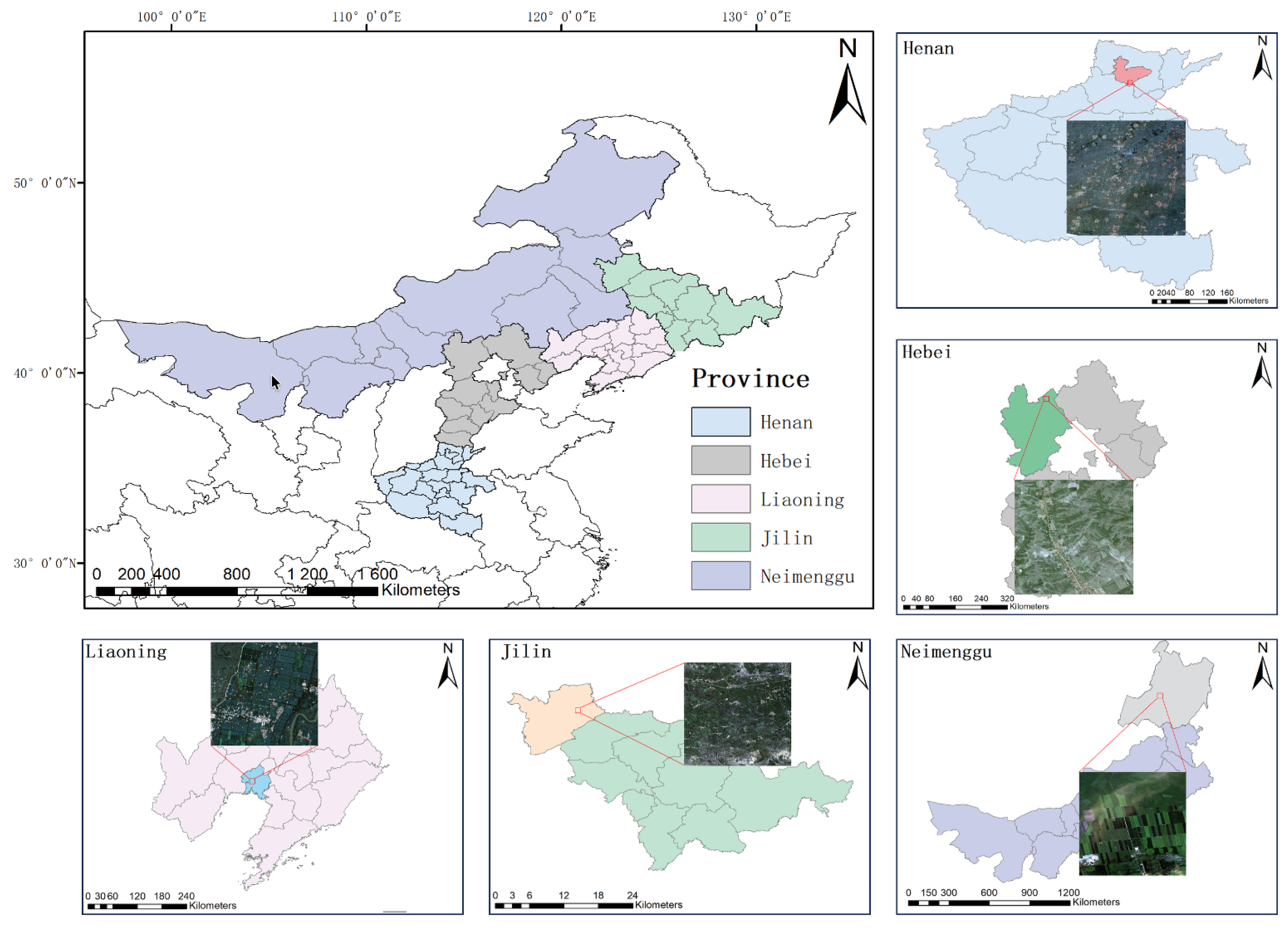
This study focuses on five representative agricultural regions in northern China: Hebi City in Henan Province, Zhangjiakou City in Hebei Province, Panjin City in Liaoning Province, Da’an City in Jilin Province, and Hulunbuir City in Inner Mongolia, as shown in Figure 1. These regions were selected to cover diverse crop types, planting structures, terrains, and climatic conditions, providing a representative test for evaluating spatial–spectral complementarity under heterogeneous agricultural scenarios.

• Hebi City, Henan Province (Study Area HB): The terrain predominantly consists of flat and hilly landscapes, characterized by a warm temperate semi-humid monsoon climate. Corn is the dominant crop, typically planted in late June and harvested in October.
• Zhangjiakou City, Hebei Province (Study Area ZJK): The region predominantly features a plateau terrain and is characterized by a temperate continental monsoon climate. The primary crops cultivated are corn and potato. Corn is planted in late April and attains maturity in October, while potato are sown in late April and harvested in the same month of October.
• Panjin City, Liaoning Province (Study Area PJ): The predominant terrain is characterized by flatland, subjected to a temperate monsoon climate. The primary crops cultivated are corn and rice. Corn is typically sown in early May and harvested in October, while rice is transplanted in May and harvested in early October.
• Da’an City, Jilin Province (Study Area DA): The terrain is predominantly flat and characterized by a temperate continental monsoon climate. The primary crops cultivated are corn and rice. Corn is sown in early May and harvested in October, while rice is transplanted in May and harvested in early October.
• Hulunbuir City, Inner Mongolia (Study Area HLBE): The terrain is characterized by plateaus, mountains, and plains, and experiences a climate that integrates the features of both temperate continental monsoon and temperate steppe climates.The main crops in this region are corn, wheat, and potato. Corn is planted in late April and matures in September; wheat is planted in March and matures in August; and potato are planted in early May and mature in August.

The five study areas collectively reflect the diversity of crop types, growth patterns, and environmental conditions in northern China. Phenological characteristics play an important role in crop identification; however, this study does not explicitly model temporal dynamics.

As shown in

Table 1. Fertility periods of major crops in the study area.

Study Area	Crop	Cropping System	Sowing/Emergence	Growth	Maturity/Harvest
HB	Winter wheat	Winter crop	M Oct.	Nov.—M May.	L May.—M Jun.
	Summer maize	Double cropping	M Jun.	Jul.—Aug.	M Sep.—M Oct.
ZJK	Maize	Spring crop	L Apr., M May.	Jun.—Aug.	M Sep., E Oct.
	Potato	Spring crop	M Apr., M May.	Jun.—Jul.	E Aug., M Sep.
PJ	Rice	Single crop	M Apr., M May.	Jun.—Aug.	M Sep., M Oct.
DA	Maize	Spring crop	L Apr., M May.	Jun.—Aug.	M Sep., M Oct.
	Rice	Single crop	M Apr., M May.	Jun.—Aug.	E Sep., L Sep.
HLBE	Spring wheat	Spring crop	M Apr., M May.	Jun.—Jul.	M Aug., E Sep.
	Maize	Spring crop	E May.	Jun.—Aug.	E Sep., L Sep.
	Potato	Spring crop	E May.	Jun.—Jul.	E Aug., M Sep.

, the growth periods of major crops in the study areas are summarized, where E, M, and L denote the early, middle, and late stages of each month, respectively. It can be observed that key growth and development stages of typical crops such as corn, rice, wheat, and potato mainly occur from July to September, during which crops exhibit relatively stable and discriminative spatial and spectral characteristics. Therefore, imagery from these months was selected to ensure phenological consistency rather than to perform explicit temporal modeling.

2.2. Remote Sensing Data

This study employs optical remote sensing imagery acquired from the GF-2 and Sentinel-2 satellites. GF-2 is a high-resolution Earth observation satellite developed by China. Equipped with two imaging sensors, it includes a 1 m panchromatic sensor and a 4 m multi-spectral sensor consisting of four spectral bands (blue, green, red, and near-infrared). GF-2 data used in this study were obtained from the National Remote Sensing Data and Application Service Platform(CPEOS) https://www.cpeos.org.cn. Standard preprocessing steps, including orthorectification, geometric registration, and pan-sharpening, were applied to generate multi-spectral imagery at a spatial resolution of 1 m.

In addition, multi-spectral imagery from the Sentinel-2 constellation operated by the European Space Agency was used to provide complementary spectral information. The Sentinel-2 system consists of two satellites, each carrying a multi-spectral instrument with 13 spectral bands, achieving a nominal revisit period of five days. Sentinel-2 Level-2A products can be publicly accessed via the Google Earth Engine (GEE) platform. Images acquired at dates close to the corresponding GF-2 acquisition times were selected to ensure temporal consistency. After cloud screening, mosaicing, and spatial cropping, Sentinel-2 imagery covering the study areas was obtained. For regions with persistent cloud contamination, including PJ and HLBE, monthly composite images were used instead.

It is worth noting that, due to its wider swath and higher revisit frequency, Sentinel-2 imagery provides greater flexibility for temporal sampling. In this study, however, Sentinel-2 data are primarily utilized for their rich spectral information, while temporal analysis is left for future extensions.

In some regions (e.g., PJ), exact temporal alignment between GF-2 and Sentinel-2 imagery is constrained by cloud contamination and data availability. The selected Sentinel-2 images still correspond to the main crop growth season and provide stable spectral characteristics for crop discrimination.

The multi-spectral information provided by Sentinel-2 offers significant advantages for crop identification due to the distinct spectral reflection characteristics of vegetation in the visible, red-edge, near-infrared, and shortwave infrared wavelengths. Based on an analysis of band sensitivity for crop discrimination, ten Sentinel-2 spectral bands were selected for subsequent experiments, as summarized in

Table 2. Details of utilized Sentinel-2 bands.

Band	Name	Wavelength (nm)	Resolution (m)
Band 2	Blue	490	10
Band 3	Green	560	10
Band 4	Red	665	10
Band 5	Veg Red Edge	705	20
Band 6	Veg Red Edge	740	20
Band 7	Veg Red Edge	783	20
Band 8	NIR	842	10
Band 8A	Veg Red Edge	865	20
Band 11	SWIR	1610	20
Band 12	SWIR	2190	20

. Sentinel-2 data were geometrically registered to GF-2 imagery. The purpose of controlling acquisition time is to reduce phenological-induced appearance variations, rather than to model crop growth trajectories. The acquisition dates of both GF-2 and Sentinel-2 imagery for each study area are listed in

Table 3. Remote sensing data acquisition information for different study areas.

Sensor	Study Area	Acquisition Time (Year/Month/Day)
GF-2	HB	2022/07/01
	ZJK	2021/07/11
	PJ	2021/09/12
	DA	2021/09/12
	HLBE	2021/07/21
Sentinel-2	HB	2022/07/01
	ZJK	2021/07/11
	PJ	2021/05
	DA	2021/09/23
	HLBE	2021/06

.

2.3. Reference Samples

A set of labeled reference samples to support model training and quantitative evaluation was constructed in the study. The reference samples were generated through a combination of field survey records and visual interpretation based on high-resolution Google Earth imagery, conducted by experts in a controlled office environment.

During the labeling process, meter-level high-spatial-resolution images from Gaofen-2 (GF-2) were used as the primary reference base map for delineating crop parcels and assigning crop types. The labeled samples were distributed across five study areas in northern China and covered five crop categories: corn, rice, wheat, potato, and others.

In total, 10,680 parcel samples were labeled, including 6011 corn samples, 1988 rice samples, 855 wheat samples, 1334 potato samples, and 492 samples of other crop types. The spatial distribution and statistical summary of the labeled samples across different study areas are reported in

Table 4. Statistical summary of labeled crop samples in different study areas.

Study Area	Corn	Rice	Wheat	Potato	Others	Total
HB	3945	0	0	0	0	3945
ZJK	16	0	0	1146	0	1162
PJ	21	1726	0	0	0	1737
DA	1791	262	0	0	145	2198
HLBE	238	0	855	188	347	1628
Total	6011	1988	855	1334	492	10,680

.

2.4. SSCR-Agri

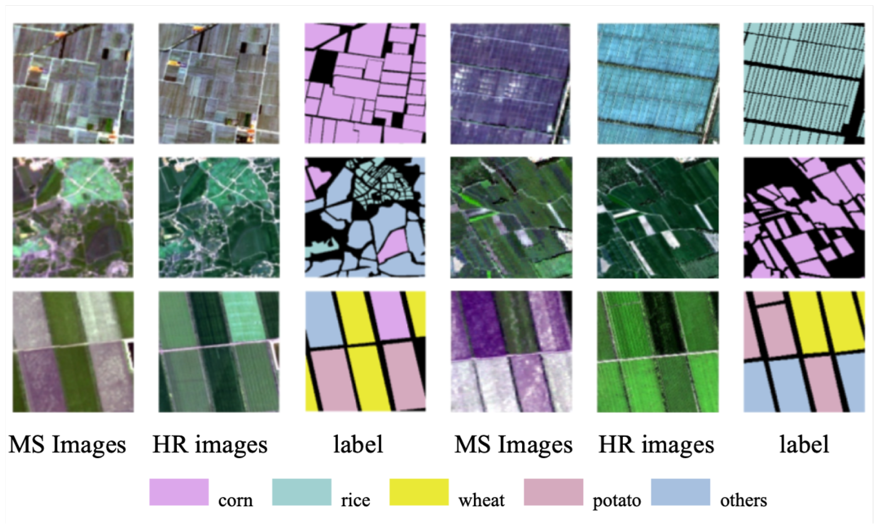
To investigate cross-resolution spatial–spectral fusion for fine-grained crop classification, we constructed the Spatial–Spectral Complementary Resolution Agricultural Dataset (SSCR-Agri). The dataset integrates meter-level high spatial resolution imagery from Gaofen-2 (GF-2) and coarser-resolution multi-band imagery from Sentinel-2, covering representative agricultural regions in northern China. In order to facilitate pixel-wise learning and cross-source alignment, Sentinel-2 images were upsampled to a spatial resolution of 1 m and geometrically aligned with the GF-2 imagery. It should be noted that this upsampling operation is performed solely for spatial alignment purposes, while the original spectral characteristics of Sentinel-2 are preserved.

Each data sample in SSCR-Agri has a spatial size of $1000\times 1000$ pixels at 1m resolution and consists of three components: (1) GF-2 images, as high-resolution (HR) imagery providing fine-grained spatial structural information, (2) Sentinel-2 multi-band images, as coarser multi-spectral (MS) imagery, providing complementary spectral cues, and (3) corresponding crop labels. The dataset includes five crop categories: corn, rice, wheat, potato, and others.

The SSCR-Agri dataset is divided into training and test subsets with a ratio of 7:3, containing 1229 training samples and 528 test samples, respectively, for a total of 1757 image patches. An example of the SSCR-Agri dataset is illustrated in Figure 2.

The processed dataset and related experimental resources can be obtained upon reasonable request.

3. Methodology

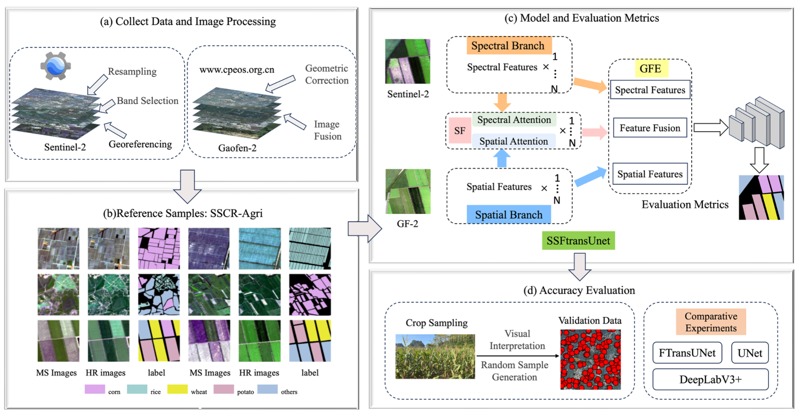
The construction of accurate spatial and spectral features is critical to fine crop classification. This study integrates high-resolution images and multi-spectral coarser images to derive high-resolution spatial features and multi-band spectral features from various data sources, addressing the limitations of high spatial resolution crop fine classification data. To address these challenges, this research proposes a Spectral-Spatial Feature Fusion TransUNet (SSF-TransUnet) specifically tailored for intricate crop classification tasks. The technical methodology is illustrated in Figure 3: GF and Sentinel images are collaboratively employed to generate a comprehensive dataset for precise crop classification (SSCR-Agri) through geospatial registration and resampling techniques. The SSF-TransUnet is designed with two parallel branches: one branch learns spatial features, such as field texture and field boundary characteristics, while the other branch identifies spectral features, such as crop spectra and their differences. The results were analysed and experimentally verified subsequently.

3.1. SSF-TransUnet

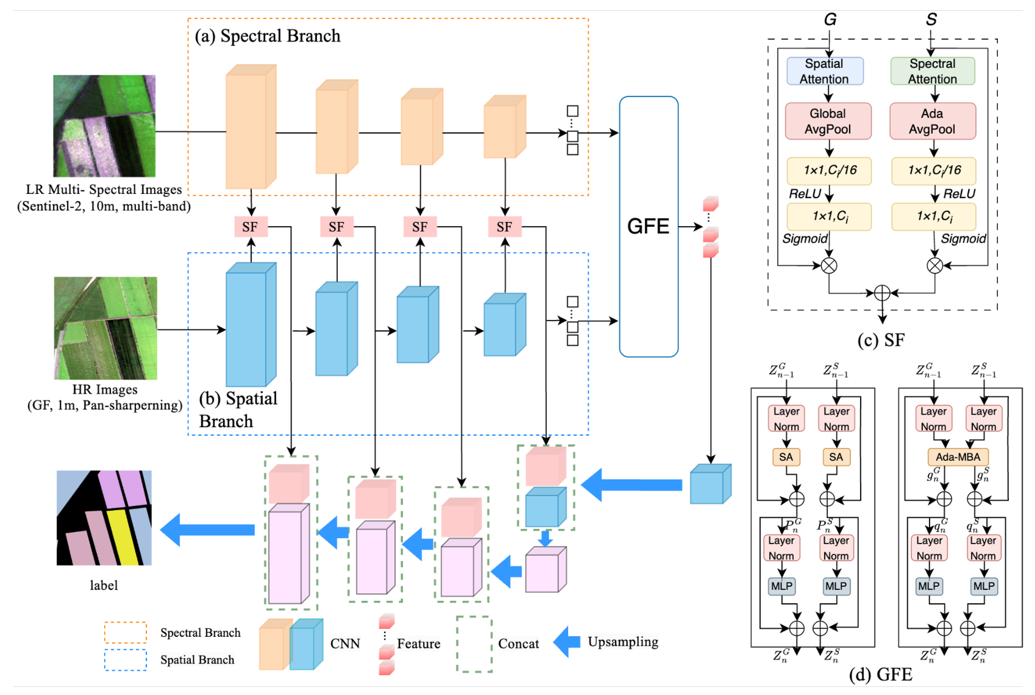
The SSF-TransUnet network architecture proposed in this study is shown in Figure 4. The model consists of four main components: the Spectral branch, the Spatial branch, the Spectral-Spatial Feature Fusion (SF) module, and the Global Feature Extraction (GFE) module. The Spectral branch and Spatial branch are responsible for extracting the crop spectral features and the spectral feature differences between crops from the MS images, as well as the spatial information of farmland textures and field boundaries from the GF images. The SF module integrates the spectral information from the Sentinel images and the spatial information from the GF images. The GFE module extracts deep information from both image sources, achieving feature retention and fusion learning of spatial and spectral features. In the proposed SSF-TransUnet, two ResNet branches are used to extract features from the spectral input and the spatial input.

3.1.1. Spectral Branch and Spatial Branch

In this study, $S\in {\mathbb{R}}^{H\times W\times 10}$, $G\in {\mathbb{R}}^{H\times W\times 4}$, denote the multi-spectral (MS) input and the high-resolution (HR) input, respectively, where H and W are the height and width of the input, S has 10 channels, and G has 4 channels, as shown in Figure 4a,b. The SSF-TransUnet adopts the dual-branch encoder architecture of FTransUnet [32]. The Spectral branch extracts spectral information from S, while the Spatial branch extracts spatial information from G. The encoder branches consist of four convolutional layers for multi-scale information extraction, with dimensions $C_i\times \left(H/2^{i-1}\right)\times \left(W/2^{i-1}\right)$, where i is the layer index of the CNN encoder. These shallow features are fused through the SF module, which combines the features extracted by convolution operations, and the fused information is passed to the next S encoder branch.

The spectral branch and spatial branch adopt independent encoder parameters and process multi-spectral (MS) and high-resolution (HR) inputs separately. The encoder structure follows the common four-stage design widely adopted in UNet-like architectures and ResNet backbones, which enables multi-scale feature extraction while maintaining computational efficiency. Feature interaction between the two branches is performed at multiple encoder stages through the proposed spatial–spectral fusion (SF) modules. The fused features are then propagated to the decoder through skip connections following the U-Net architecture, enabling the integration of multi-level spatial–spectral information. During training, the entire network is optimized end-to-end via backpropagation, allowing gradients to flow through both branches and the fusion modules simultaneously.

3.1.2. SF Module

The SF module employs spectral attention in the Spectral Branch and spatial attention in the Spatial Branch to extract spectral and spatial information from the S and G branches. Global information is aggregated using Global Average Pooling (AvgPool). Given the input channel dimension $C_i$ of the i-th SF module, the process involves AvgPool followed by two 1 × 1 convolutional operations, ReLU activation, and a Sigmoid function. The features from the S and G branches are then weighted and combined through element-wise summation, producing fused shallow features as output. The architecture is illustrated in Figure 4c.

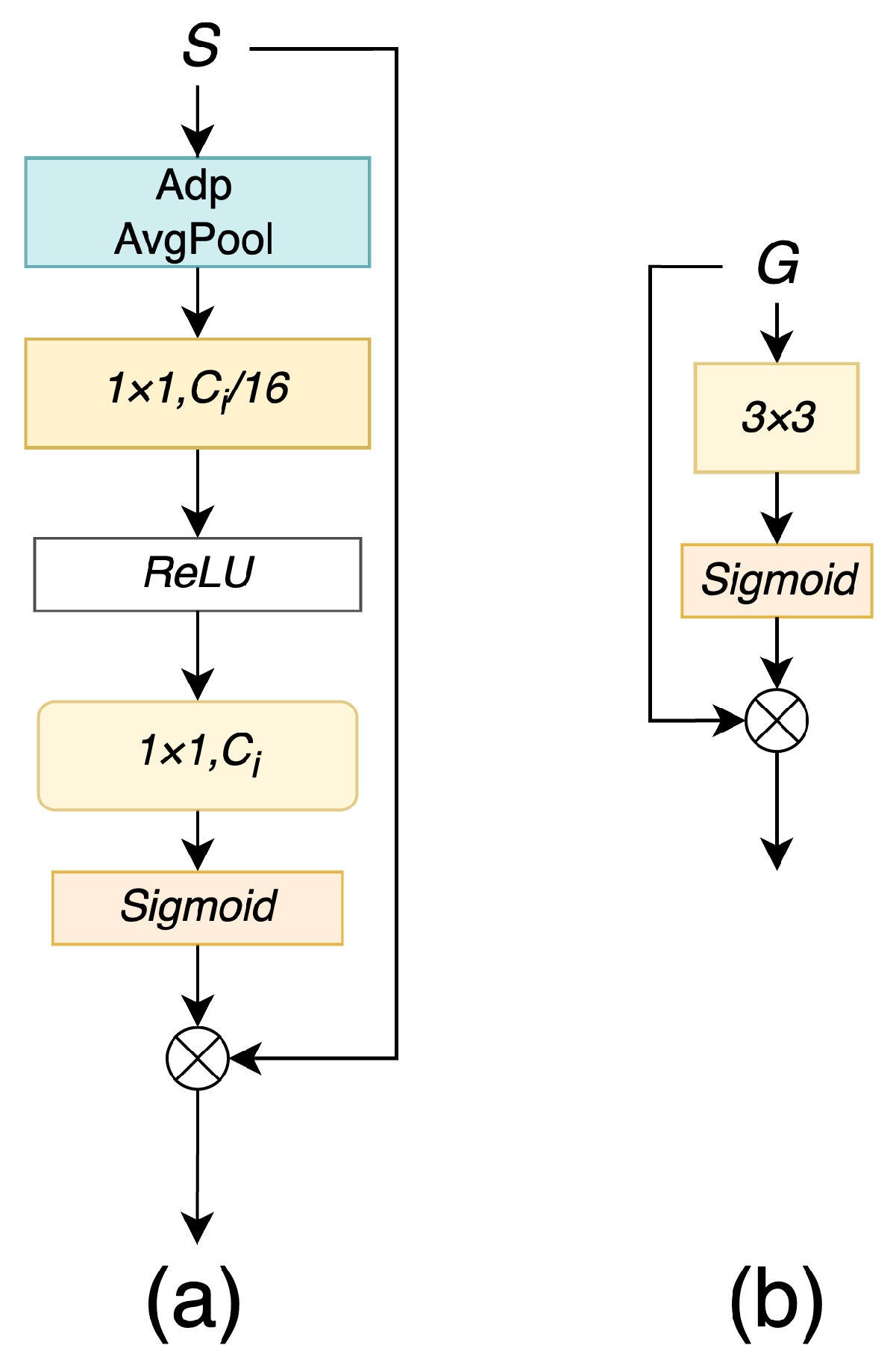
The spectral attention performs adaptive average pooling on the input feature map $S\in {\mathbb{R}}^{H\times W\times 10}$. The first convolutional layer reduces the number of channels from C to $C/16$, followed by a ReLU activation function. The second convolutional layer then increases the number of channels from $C/16$ to C, and a Sigmoid activation function is applied to obtain the spectral attention weights. Finally, the original input feature map S is multiplied by the spectral attention weights, resulting in the output feature map. For spatial attention, the input feature map $G\in {\mathbb{R}}^{H\times W\times 4}$ undergoes a 3 × 3 convolution operation. The resulting feature map is passed through a Sigmoid activation function to obtain the spatial attention weights. The original input feature map G is then multiplied by the spatial attention weights, producing the output feature map, as shown in Figure 5.

3.1.3. GFE Module

The GFE module is designed to capture deeper cross-modal relationships between spatial and spectral features through attention-based interaction. Together with the SF module, it enables effective multi-level spatial–spectral feature integration within the proposed architecture. The input of the GFE passes through three processes: deep feature enhancement by the self-attention (SA) layer, deep feature fusion by the Ada-MBA layer, and feature enhancement fusion by another SA layer. The layers are denoted by $N_1$, $N_2$ and $N_3$. Let $Z_n^S$ and $Z_n^G$ respectively represent the hidden features at the n-th layer of the S and G branches, where $n\in \{1,2,\dots ,N_1+N_2+N_3\}$. The SA layer consists of two SA modules, an MLP module, and Layer Norm. This process is illustrated in Figure 4d.

Given the feature inputs represented by $Z_{n-1}^S$ and $Z_{n-1}^G$, the SA layer is designed to derive the global relationships of each input using the mechanism proposed in [27]. When $n=1,2,3$, the output of the n-th layer SA is:

$$P_n^S=SA\left(LN\left(Z_{n-1}^S\right)\right)+Z_{n-1}^S$$

(1)

$$P_n^G=SA\left(LN\left(Z_{n-1}^G\right)\right)+Z_{n-1}^G$$

(2)

$$Z_n^S=MLP\left(LN\left(P_n^S\right)\right)+P_n^S$$

(3)

$$Z_n^G=MLP\left(LN\left(P_n^G\right)\right)+P_n^G$$

(4)

After the deep feature enhancement by the SA layer, the Global Feature Extraction (GFE) module utilizes $Ada-MBA$ layers to fuse the features with contextual information. The output formula of the Ada-MBA layer is as follows:

$$(g_n^S,g_n^G)=Ada-MBA(LN\left(Z_{n-1}^S\right),LN\left(Z_{n-1}^G\right))$$

(5)

Let $q_n^S=g_n^S+Z_{n-1}^S$ and $q_n^G=g_n^G+Z_{n-1}^G$. When $n=4,5,...$, the fusion output of the N layer is:

$$Z_n^S=MLP\left(LN\left(q_n^S\right)\right)+q_n^S$$

(6)

$$Z_n^G=MLP\left(LN\left(q_n^G\right)\right)+q_n^G$$

(7)

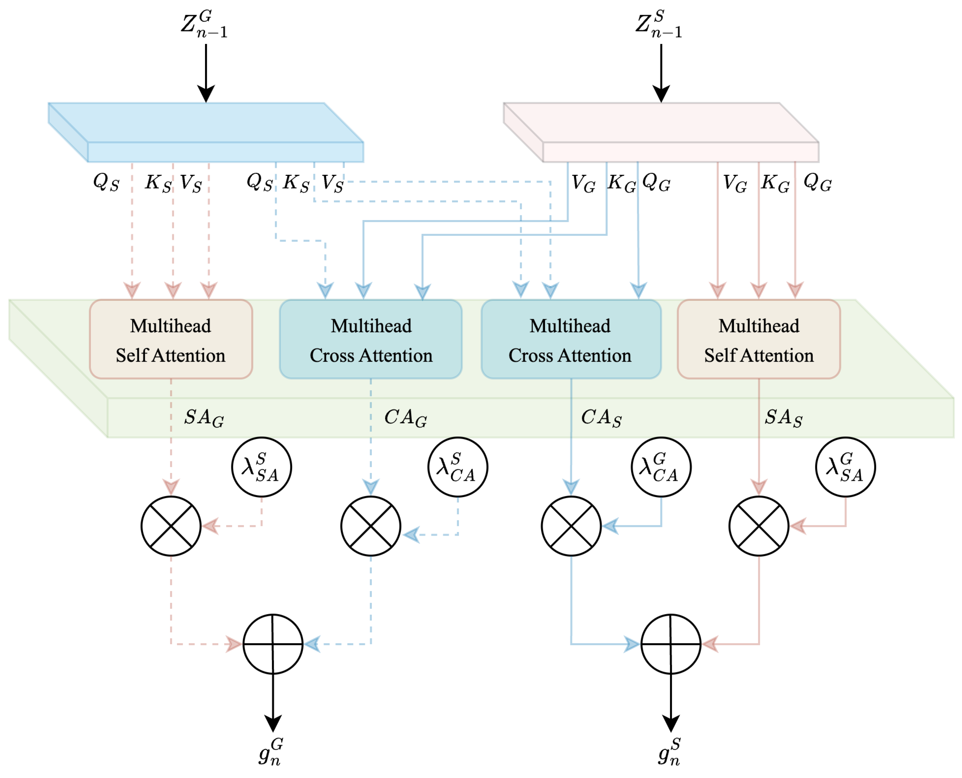
The structure of the Ada-MBA module divides $Z_{n-1}^S$ and $Z_{n-1}^G$ into $N_h$ equal-length segments, represented as $Z_{n-1,h}^S$ and $Z_{n-1,h}^G$, where $h=1,2,...,N_h$, as shown in Figure 6.

The two sets of matrices $Q_G,K_G,V_G$, and $Q_S,K_S,V_S$, are calculated using linear projections $U_{qkv}^S$ and $U_{qkv}^G$. For the two modes, the Self-Attention (SA) information (${SA}_G$ and ${SA}_S$) and Cross-Attention (CA) information (${CA}_G$ and ${CA}_S$) are derived, where $\mathrm{Softmax}(·)$ is applied row-wise to the similarity matrix. SA uses $Q_S,K_S,V_S$ and $Q_G,K_G,V_G$ to compute the internal information, while CA uses $Q_S,K_G,V_G$ and $Q_G,K_S,V_S$ to compute cross-modal information. This approach enables the extraction and fusion of deep features. The flow in the Ada-MBA module is represented as:

$$[Q_S,K_S,V_S]=Z_{(}{n-1)}^S{U}_{\mathit{qkv}}^S$$

(8)

$$[Q_G,K_G,V_G]=Z_{(}{n-1)}^G{U}_{\mathit{qkv}}^G$$

(9)

$$S{A}_G=\mathrm{Softmax}({\displaystyle \frac{Q_G{K}_G^T}{\sqrt{d}}})V_G$$

(10)

$$S{A}_S=\mathrm{Softmax}({\displaystyle \frac{Q_S{K}_S^T}{\sqrt{d}}})V_S$$

(11)

$$C{A}_G=\mathrm{Softmax}({\displaystyle \frac{Q_S{K}_G^T}{\sqrt{d}}})V_G$$

(12)

$$C{A}_S=\mathrm{Softmax}({\displaystyle \frac{Q_G{K}_S^T}{\sqrt{d}}})V_S$$

(13)

The following adaptive mechanisms are used to fuse $SA$ and $CA$:

$$g_n^G={\lambda }_{SA}^{G}S{A}_G+{\lambda }_{CA}^{G}C{A}_G$$

(14)

$$g_n^S={\lambda }_{SA}^{S}S{A}_S+{\lambda }_{CA}^{S}C{A}_S$$

(15)

Finally, the fused feature maps are enhanced separately for the S and G branches.

3.2. Evaluation Metrics

The pixel-level accuracy is used as the evaluation criterion in this study. The Intersection over Union (IoU), mean IoU (mIoU) and Overall Accuracy (OA) were used to evaluate the performance of the proposed and compared methods. OA assesses global accuracy regardless of individual categories, reflecting the classification overall accuracy for all categories. IoU is defined as the ratio between the intersection and union of predicted pixels for a specific class and the corresponding ground truth pixels. The three evaluation indexes are given as follows:

$$OA={\displaystyle \frac{{\sum }_{i=1}^{N}C{M}_{ii}}{{\sum }_{i=1}^N{\sum }_{j=1}^{N}C{M}_{ij}}}$$

(16)

where $C{M}_{ii}$ denotes the elements of row i, column i of the confusion matrix (the number of pixels in which the i category was correctly categorized), and $C{M}_{ij}$ denotes the elements of row i, column j of the confusion matrix (i.e., the number of pixels that were actually category j but were predicted to be category i).

$$IoU={\displaystyle \frac{T{P}_i}{T{P}_i+F{P}_i+F{N}_i}}$$

(17)

$T{P}_i$ is the number of pixels for which the i category was correctly categorized (true positives). $f{p}_i$ is the number of pixels that were incorrectly predicted to be the i category (false positives). $f{n}_i$ is the number of pixels that were actually the i category but incorrectly predicted to be some other category (false negatives). In the confusion matrix, $T{P}_i$ is the elements on the diagonal, $F{P}_i$ is the sum of the elements in the i non-diagonal row, and $F{N}_i$ is the sum of the elements in the i non-diagonal column.

$$mIoU={\displaystyle \frac{{\sum }_{i=1}^{N}Io{U}_i}{N}}$$

(18)

N is the number of categories. $Io{U}_i$ is the IoU value of the i category. IoU and mIoU are widely used evaluation metrics in semantic segmentation tasks because they incorporate both false positives and false negatives and provide balanced evaluation across classes.

4. Experiments

4.1. Experimental Settings

All experiments were conducted using the 2.1.0 version PyTorch deep learning framework on a single NVIDIA RTX 3090 GPU. Stochastic Gradient Descent (SGD) was adopted as the optimizer with an initial learning rate of 0.01, and all models were trained for 50 epochs. Model weights were saved after each epoch.

To ensure fair comparison, all methods were trained and evaluated using the same training and test splits, identical input patch sizes, and consistent optimization settings. No model-specific hyperparameter tuning was performed, and no additional post-processing was applied to the classification results.

4.2. Overall Performance on Study Areas

This study evaluates the overall performance of the proposed SSF-TransUnet across five representative agricultural regions in northern China, including HB, ZJK, PJ, DA, and HLBE. These regions differ in crop composition, planting structures, and environmental conditions, providing a comprehensive test of model robustness.

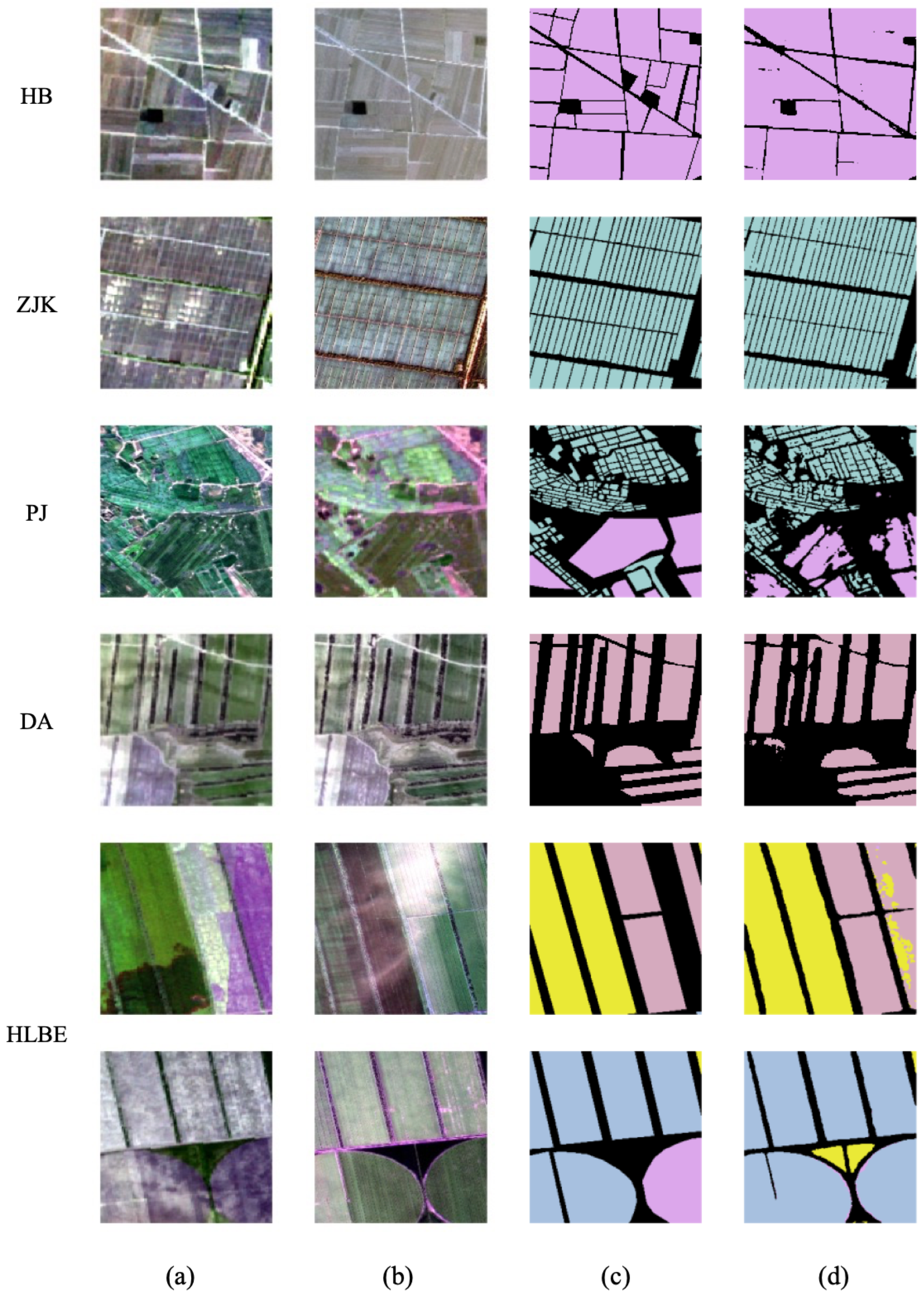
Figure 7 presents qualitative classification results for each study area. The rows correspond to different regions, illustrating spatial distributions of predicted crop types in comparison with reference labels. The results demonstrate that SSF-TransUnet is capable of accurately delineating crop boundaries and preserving fine-grained spatial structures across diverse agricultural scenarios.

Quantitative evaluation results are summarized in

Table 5. Statistical table of precision indicators for fine analysis of crops in different regions.

Study Area	IoU					mIoU	OA (%)
	Corn	Rice	Wheat	Potato	Others
HB	0.97	–	–	–	–	0.194	97.01
ZJK	–	–	–	0.7357	–	0.1471	69.86
PJ	0.744	0.6947	–	–	0.1538	0.3185	89.52
DA	0.7441	–	–	–	–	0.1488	71.78
HLBE	0.9923	–	0.6993	0.5694	0.4277	0.5377	60.79

. The proposed method achieves high classification accuracy across most regions, with consistently strong performance for dominant crop types such as corn and rice. It should be noted that some crop classes are absent in certain study areas. Due to the heterogeneous crop distributions among different regions and the absence of certain classes in some areas, the regional mIoU is reported only as a reference, while the class-wise IoU provides a more informative evaluation of the classification performance for each crop type.

4.3. Comparison with Baseline Methods

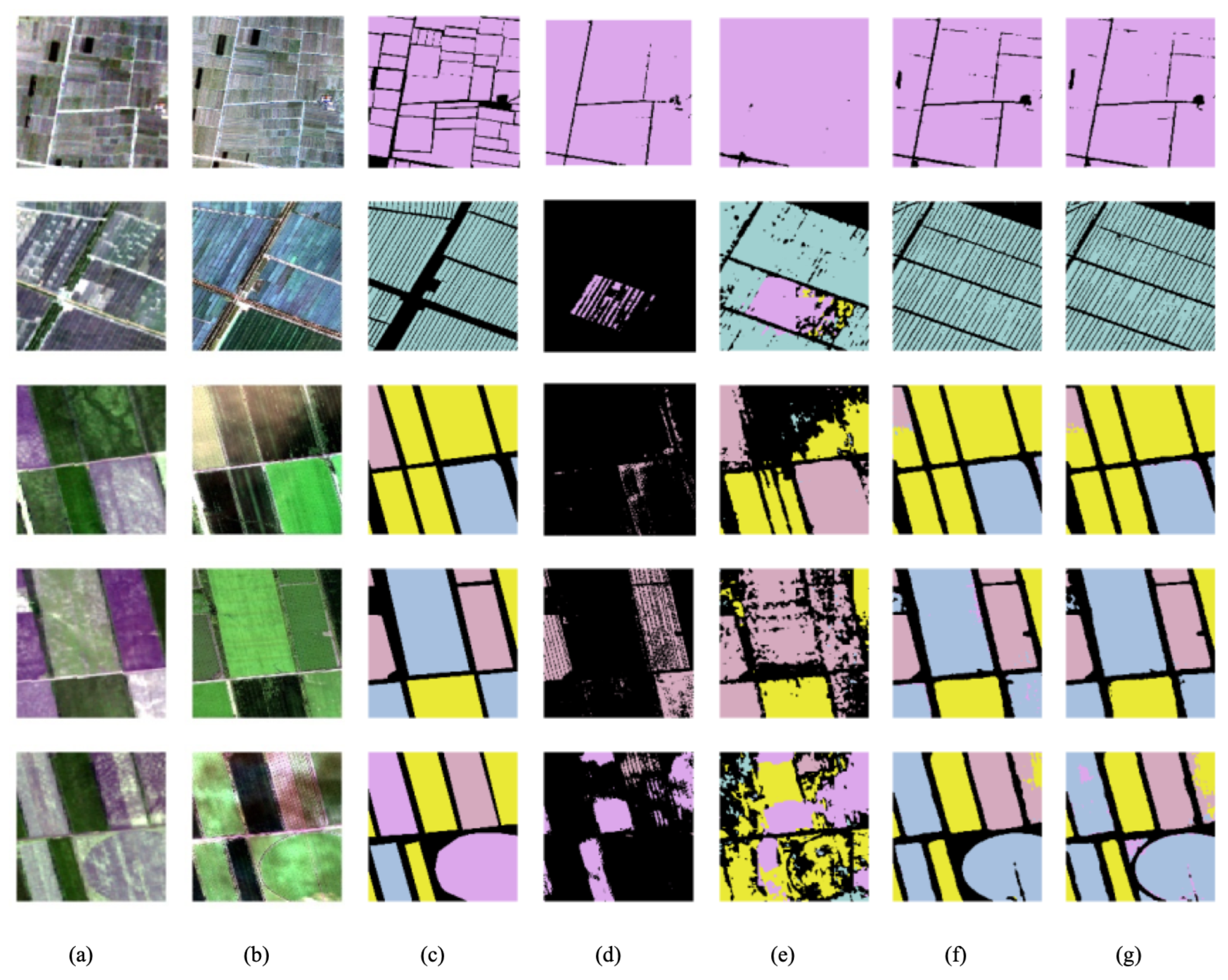
To demonstrate the effectiveness and competitiveness of the proposed SSF-TransUnet, comparative experiments were conducted against representative semantic segmentation models, including UNet [34], DeepLabV3+ [35], and FTransUNet [32]. These models represent classical convolutional architectures and hybrid CNN–Transformer designs commonly used in remote sensing image segmentation. It should be noted that the main objective of this study is to investigate cross-source spatial–spectral fusion rather than to explore different backbone architectures. Therefore, the backbone network is fixed across experiments to ensure fair comparison among different fusion strategies. UNet represents a classical CNN-based encoder–decoder segmentation architecture that focuses on local spatial feature extraction through convolution and skip connections. DeepLabV3+ extends CNN-based segmentation with atrous convolution and multi-scale context modeling, while FTransUNet represents a hybrid CNN–Transformer framework that introduces global attention mechanisms for long-range dependency modeling.

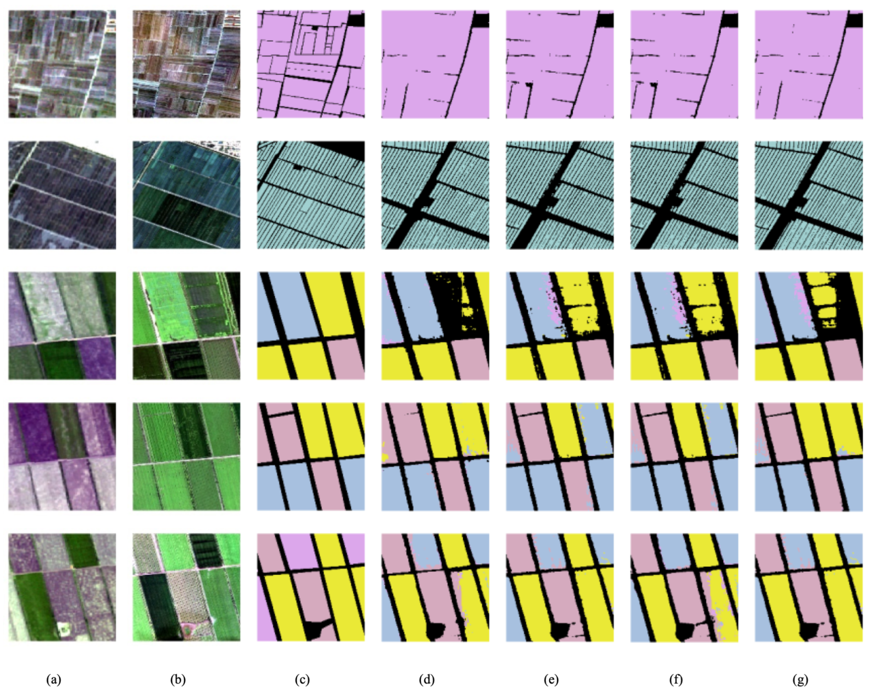
Figure 8 provides a visual comparison of classification results produced by different models on selected image patches. UNet exhibits notable misclassification and omission errors, particularly along crop boundaries. DeepLabV3+ improves overall recognition performance but still suffers from boundary ambiguity. FTransUNet captures most crop categories but lacks fine boundary precision in complex agricultural scenes. In contrast, SSF-TransUnet produces more coherent classification maps with clearer field boundaries and fewer misclassifications.

Quantitative comparison results are reported in

Table 6. Evaluation of the accuracy of classification results.

Model	Params (M)	IoU					mIoU	OA (%)
		Corn	Rice	Wheat	Potato	Others
Unet	31.0	0.7165	0.6217	0.396	0.3571	0.0643	0.2147	51.6
DeeplabV3+	39.6	0.8426	0.7977	0.4957	0.5719	0.0503	0.5516	65.48
FTransUnet	54.3	0.8215	0.865	0.6645	0.6848	0.2972	0.6666	79.65
SSF-TransUnet	56.1	0.9111	0.9343	0.823	0.8247	0.532	0.805	81.84

. SSF-TransUnet achieves the highest overall accuracy (OA) and mean Intersection over Union (mIoU), reaching 81.84% and 0.6954, respectively. Compared with UNet, DeepLabV3+, and FTransUNet, SSF-TransUnet shows consistent improvements across multiple crop categories, confirming its superior performance in fine-grained crop classification. To further evaluate the computational efficiency of the proposed method, the number of trainable parameters of different models is compared. SSF-TransUnet is in similar parameter quantity with baseline models.

4.4. Effectiveness of Spectral-Spatial Joint Utilization

To further investigate the contribution of spatial–spectral joint utilization, additional experiments were conducted by varying the input data sources while keeping the network architecture unchanged. Three input configurations were evaluated: (1) multi-spectral images only, (2) high-resolution images only, and (3) joint utilization of both spatial and spectral information.

The quantitative results of these experiments are summarized in

Table 7. Evaluation of accuracy of spectral-spatial characterization. ✓ and × indicate that the corresponding data source is used or not used, respectively. MS images refer to multispectral images, and HR images denote high-resolution images.

	IoU					mIoU	OA (%)
	Corn	Rice	Wheat	Potato	Others
✓ MS images × HR images	0.7989	0.8244	0.6281	0.6166	0.3122	0.636	76.78
× MS images ✓ HR images	0.8383	0.8403	0.5836	0.6398	0.3333	0.647	78.84
✓ MS images ✓ HR images	0.9111	0.9343	0.823	0.8247	0.532	0.805	81.84

. When spatial and spectral information are jointly utilized, the model achieves consistently higher IoU scores across all crop categories compared with single-source inputs. The joint-input configuration attains an mIoU of 0.6954 and an OA of 81.84%, outperforming both multi-spectral-only and spatial-only settings.

These results indicate that spatial and spectral information provide complementary cues for crop classification, and their joint utilization leads to more accurate and stable predictions across diverse crop types and regions.

5. Discussion

5.1. Structural Necessity of Spatial–Spectral Joint Features

The experimental results indicate that jointly utilizing spatial and spectral information consistently leads to improved crop classification performance compared with using either information source alone (Table 7). This phenomenon is closely related to the intrinsic characteristics of fine-grained crop segmentation tasks.

Agricultural parcels exhibit strong internal spatial consistency, with relatively homogeneous appearance within a field and sharp transitions at field boundaries. High spatial resolution imagery is therefore essential for preserving field geometry and boundary integrity. However, crops with similar planting patterns and field shapes often remain difficult to distinguish when relying solely on spatial cues. Conversely, spectral information encodes crop-specific biochemical and physiological properties, enabling discrimination between visually similar crops, yet its coarser spatial resolution and mixed-pixel effects may blur fine boundary details. Although boundary-aware metrics could provide additional insights into segmentation behavior, the objective of this study is multi-class crop classification rather than explicit field boundary extraction. Object-based pipelines, which first segment field boundaries and then perform parcel-level classification, provide an alternative paradigm for agricultural mapping. However, such approaches require reliable parcel boundaries and may suffer from error propagation between stages. In contrast, the proposed framework performs end-to-end spatial–spectral feature learning directly at the pixel level.

These complementary characteristics make spatial–spectral joint modeling structurally necessary for fine crop classification. Effective segmentation requires both accurate boundary delineation and reliable crop-type discrimination. The consistent performance gains observed when MS images and HR images are jointly used suggest that spatial and spectral features provide non-redundant information that cannot be fully captured by single-source inputs.

Although variations in crop composition and regional planting complexity may influence the absolute classification accuracy, these factors do not alter the fundamental necessity of jointly modeling spatial structures and spectral characteristics for fine-grained crop segmentation.

5.2. Role of Spectral Band Complementarity in Crop Discrimination

The band-level experiments further elucidate how spectral diversity contributes to fine-grained crop classification (Figure 9 and

Table 8. Evaluation of band feature accuracy.

Band	IoU					mIoU	OA(%)
	Corn	Rice	Wheat	Potato	Others
(d) Main and Auxiliary Branches interchanged	0.8351	0.8724	0.6711	0.7277	0.347	0.6907	81.74
(e) Gray Scale of HR images Only	0.8219	0.849	0.686	0.6516	0.2952	0.6608	79.09
(f) Near Infrared Band of HR images Only	0.833	0.878	0.683	0.6512	0.2902	0.667	80.74
(g) Our selected bands	0.9111	0.9343	0.823	0.8247	0.532	0.805	81.84

). Results obtained using simplified spectral representations, such as grayscale imagery or a single near-infrared band, demonstrate reduced discriminative capability, particularly for crops with overlapping phenological characteristics.

While dominant crops such as corn and rice can often be identified with limited spectral information, more challenging categories—including wheat, potato, and mixed “others”—require richer spectral cues for reliable separation. Multi-band spectral inputs capture complementary information related to vegetation structure, chlorophyll content, and moisture conditions, which are critical for distinguishing crops with similar spatial appearances.

The superior performance achieved by the full spectral configuration indicates that effective crop classification relies not on individual bands, but on the complementary interaction among multiple spectral channels. These findings highlight the importance of incorporating rich spectral representations into spatial–spectral frameworks, especially in complex agricultural environments.

5.3. Effectiveness of the Dual-Branch Architecture and Attention Mechanisms

To analyze the contribution of different components in the proposed architecture, we conduct an ablation study by selectively enabling or disabling the spatial attention and spectral attention modules. The ablation experiments provide insight into the contribution of the proposed architectural components (

Table 9. Ablation study: evaluation of classification accuracy of different module combinations. ✓ indicates that the corresponding module is enabled.

Spatial Attention	Spectral Attention	mIoU	OA (%)
		0.6666	79.65
✓		0.6826	80.15
	✓	0.6839	80.93
✓	✓	0.805	81.84

). Removing either spatial attention or spectral attention results in a noticeable decline in performance, while simultaneously enabling both mechanisms yields the best overall accuracy.

Spatial attention enhances the model’s ability to focus on structurally important regions, such as crop parcels and boundary areas, promoting spatial coherence in segmentation results. Spectral attention selectively emphasizes informative spectral channels, facilitating discrimination among crops with subtle spectral differences. The combination of both mechanisms enables coordinated yet decoupled feature learning across spatial and spectral domains.

These results suggest that the performance improvements of SSF-TransUnet are not merely due to increased network complexity, but rather arise from its explicit design for spatial–spectral decoupling and interaction. The dual-branch architecture allows domain-specific features to be preserved while enabling effective cross-domain integration, which is particularly beneficial under heterogeneous resolution conditions. Also, adopting only the spectral branch yields slightly better performance, indicating that spectral information plays a more dominant role in fine-grained crop discrimination, while spatial information mainly contributes to boundary refinement.

6. Conclusions

This study investigates fine-grained crop classification from a spatial–spectral perspective and addresses the challenge of jointly exploiting heterogeneous remote sensing information under practical resolution constraints. Two main contributions are summarized as follows.

First, this study proposes SSF-TransUnet, a dual-branch spatial–spectral joint modeling framework designed to explicitly decouple and coordinate spatial structure extraction and spectral discriminability learning. By jointly utilizing high spatial resolution imagery and multi-spectral observations within a unified network architecture, the proposed method effectively preserves crop boundary integrity while enhancing crop-type separability. Extensive experiments across representative agricultural regions in northern China demonstrate that SSF-TransUnet consistently outperforms conventional CNN-based and hybrid CNN–Transformer models in fine-grained crop classification tasks.

Second, this study constructs the SSCR-Agri dataset, a spatial–spectral complementary resolution agricultural dataset integrating meter-level GF-2 imagery and multi-spectral Sentinel-2 data. The dataset covers multiple crop types and diverse agricultural environments, providing a practical benchmark for evaluating spatial–spectral joint modeling approaches. Through comprehensive qualitative and quantitative analyses, the effectiveness of joint spatial–spectral utilization is systematically validated.

Despite the promising results, several directions shows further investigation. From a modeling perspective, improving training efficiency and reducing computational cost remain important challenges when handling large-scale high-resolution remote sensing data. Future work may explore lightweight architectures and more efficient training strategies to enhance scalability. From a data perspective, expanding the dataset to include additional regions, crop types, and seasonal variations would further improve model generalization and robustness. In addition, deeper integration with ground-based observations and in-situ monitoring data could provide stronger validation and calibration of model outputs, thereby enhancing reliability for operational agricultural applications.

Overall, this study demonstrates the potential of spatial–spectral joint modeling for fine-grained crop classification and provides a solid foundation for future research in precision agriculture and large-scale agricultural monitoring.

References

1. Mirhoseini Nejad, S.M.; Abbasi-Moghadam, D.; Sharifi, A. ConvLSTM-ViT: A Deep Neural Network for Crop Yield Prediction Using Earth Observations and Remotely Sensed Data. IEEE J. Sel. Top. Appl. Earth Obs. Remote Sensed Data 2024, 17, 17489–17502. [Google Scholar]
2. Mas, M.; Broquetas, A.; Fàbregas, X.; Aguasca, A.; Llop, J.; Liu, J.; Mallorquí, J.J.; Villarroya-Carpio, A.; Lopez-Sanchez, J.M. Monitoring corn crop height and growth rate with interferometric coherence. IEEE J. Sel. Top. Appl. Earth Obs. Remote Sens. 2024, 17, 20041–20049. [Google Scholar] [CrossRef]
3. Komarek, A.M.; De Pinto, A.; Smith, V.H. A review of types of risks in agriculture: What we know and what we need to know. Agric. Syst. 2020, 178, 102738. [Google Scholar] [CrossRef]
4. Gumma, M.K.; Tummala, K.; Dixit, S.; Collivignarelli, F.; Holecz, F.; Kolli, R.N.; Whitbread, A.M. Crop type identification and spatial mapping using Sentinel-2 satellite data with focus on field-level information. Geocarto Int. 2022, 37, 1833–1849. [Google Scholar] [CrossRef]
5. Zuo, H.N.; Leng, P.; Li, Y.X.; Song, Q.; Li, Z.L. Crop mapping based on temporal and spatial sample migrations: A case study over three counties in Heilongjiang Province, Northeast China. IEEE J. Sel. Top. Appl. Earth Obs. Remote Sens. 2024, 17, 14630–14639. [Google Scholar] [CrossRef]
6. SS, V.C.; Hareendran, A.; Albaaji, G.F. Precision farming for sustainability: An agricultural intelligence model. Comput. Electron. Agric. 2024, 226, 109386. [Google Scholar] [CrossRef]
7. Belgiu, M.; Csillik, O. Sentinel-2 cropland mapping using pixel-based and object-based time-weighted dynamic time warping analysis. Remote Sens. Environ. 2018, 204, 509–523. [Google Scholar]
8. Liang, J.; Sawut, M.; Cui, J.; Hu, X.; Xue, Z.; Zhao, M.; Zhang, X.; Rouzi, A.; Ye, X.; Xilike, A. Object-oriented multi-scale segmentation and multi-feature fusion-based method for identifying typical fruit trees in arid regions using Sentinel-1/2 satellite images. Sci. Rep. 2024, 14, 18230. [Google Scholar] [CrossRef] [PubMed]
9. Sun, X.; Wang, M.; Wang, J.; Li, G.; Hou, X. Deep learning classification of winter wheat from Sentinel optical-radar image time series in smallholder farming areas. Adv. Space Res. 2024, 75, 2683–2695. [Google Scholar] [CrossRef]
10. Zhu, Z.; Qiu, S.; Ye, S. Remote sensing of land change: A multifaceted perspective. Remote Sens. Environ. 2022, 282, 113266. [Google Scholar] [CrossRef]
11. Bargiel, D. A new method for crop classification combining time series of radar images and crop phenology information. Remote Sens. Environ. 2017, 198, 369–383. [Google Scholar] [CrossRef]
12. Vuolo, F.; Neuwirth, M.; Immitzer, M.; Atzberger, C.; Ng, W. How much does multi-temporal Sentinel-2 data improve crop type classification? Int. J. Appl. Earth Obs. Geoinf. 2018, 72, 122–130. [Google Scholar] [CrossRef]
13. Savelonas, M.A.; Veinidis, C.N.; Bartsokas, T.K. Computer Vision and Pattern Recognition for the Analysis of 2D/3D Remote Sensing Data in Geoscience: A Survey. Remote Sens. 2022, 14, 6017. [Google Scholar] [CrossRef]
14. Zahir, S.A.D.M.; Omar, A.F.; Jamlos, M.F.; Azmi, M.A.M.; Muncan, J. A review of visible and near-infrared (Vis-NIR) spectroscopy application in plant stress detection. Sens. Actuators Phys. 2022, 338, 113468. [Google Scholar] [CrossRef]
15. Kumar, B.; Dikshit, O.; Gupta, A.; Singh, M.K. Feature extraction for hyperspectral image classification: A review. Int. J. Remote Sens. 2020, 41, 6248–6287. [Google Scholar] [CrossRef]
16. Qiong, H.; Wu, W.B.; Qian, S.; Miao, L.; Di, C.; Yu, Q.Y.; Tang, H.J. How do temporal and spectral features matter in crop classification in Heilongjiang Province, China? J. Integr. Agric. 2017, 16, 324–336. [Google Scholar] [CrossRef]
17. Fathololoumi, S.; Firozjaei, M.K.; Li, H.; Biswas, A. Surface biophysical features fusion in remote sensing for improving land crop/cover classification accuracy. Sci. Total. Environ. 2022, 838, 156520. [Google Scholar] [CrossRef]
18. Qiu, B.; Hu, X.; Chen, C.; Tang, Z.; Yang, P.; Zhu, X.; Yan, C.; Jian, Z. Maps of cropping patterns in China during 2015–2021. Sci. Data 2022, 9, 479. [Google Scholar] [CrossRef] [PubMed]
19. Yu, Q.; Hu, Q.; van Vliet, J.; Verburg, P.H.; Wu, W. GlobeLand30 shows little cropland area loss but greater fragmentation in China. Int. J. Appl. Earth Obs. Geoinf. 2018, 66, 37–45. [Google Scholar] [CrossRef]
20. Piiroinen, R.; Heiskanen, J.; Mõttus, M.; Pellikka, P. Classification of crops across heterogeneous agricultural landscape in Kenya using AisaEAGLE imaging spectroscopy data. Int. J. Appl. Earth Obs. Geoinf. 2015, 39, 1–8. [Google Scholar] [CrossRef]
21. Shi, D.; Yang, X. An assessment of algorithmic parameters affecting image classification accuracy by random forests. Photogramm. Eng. Remote Sens. 2016, 82, 407–417. [Google Scholar] [CrossRef]
22. Vali, A.; Comai, S.; Matteucci, M. Deep learning for land use and land cover classification based on hyperspectral and multispectral earth observation data: A review. Remote Sens. 2020, 12, 2495. [Google Scholar] [CrossRef]
23. Ma, L.; Liu, Y.; Zhang, X.; Ye, Y.; Yin, G.; Johnson, B.A. Deep learning in remote sensing applications: A meta-analysis and review. ISPRS J. Photogramm. Remote Sens. 2019, 152, 166–177. [Google Scholar] [CrossRef]
24. Lei, L.; Pan, Y.; Wang, X.; Zhong, Y.; Zhang, L. A Multi-Level Fine-Grained Crop Classification Method Based on Multi-Expert Knowledge Distill. In Proceedings of the IGARSS 2024—2024 IEEE International Geoscience and Remote Sensing Symposium; IEEE: New York, NY, USA, 2024; pp. 5044–5047. [Google Scholar]
25. Gadiraju, K.K.; Vatsavai, R.R. Remote sensing based crop type classification via deep transfer learning. IEEE J. Sel. Top. Appl. Earth Obs. Remote Sens. 2023, 16, 4699–4712. [Google Scholar] [CrossRef]
26. Yuan, Q.; Shen, H.; Li, T.; Li, Z.; Li, S.; Jiang, Y.; Xu, H.; Tan, W.; Yang, Q.; Wang, J.; et al. Deep learning in environmental remote sensing: Achievements and challenges. Remote Sens. Environ. 2020, 241, 111716. [Google Scholar] [CrossRef]
27. Dosovitskiy, A. An image is worth 16x16 words: Transformers for image recognition at scale. arXiv 2020, arXiv:2010.11929. [Google Scholar]
28. Liu, Z.; Lin, Y.; Cao, Y.; Hu, H.; Wei, Y.; Zhang, Z.; Lin, S.; Guo, B. Swin transformer: Hierarchical vision transformer using shifted windows. In Proceedings of the IEEE/CVF International Conference on Computer Vision, Montreal, QC, Canada, 10–17 October 2021; pp. 10012–10022. [Google Scholar]
29. Dong, X.; Bao, J.; Chen, D.; Zhang, W.; Yu, N.; Yuan, L.; Chen, D.; Guo, B. Cswin transformer: A general vision transformer backbone with cross-shaped windows. In Proceedings of the IEEE/CVF Conference on Computer Vision and Pattern Recognition, New Orleans, LA, USA, 18–24 June 2022; pp. 12124–12134. [Google Scholar]
30. Niu, B.; Feng, Q.; Chen, B.; Ou, C.; Liu, Y.; Yang, J. HSI-TransUNet: A transformer based semantic segmentation model for crop mapping from UAV hyperspectral imagery. Comput. Electron. Agric. 2022, 201, 107297. [Google Scholar] [CrossRef]
31. Zhang, Y.; Liu, H.; Hu, Q. Transfuse: Fusing transformers and cnns for medical image segmentation. In Proceedings of the Medical Image Computing and Computer Assisted Intervention–MICCAI 2021: 24th International Conference, Strasbourg, France, 27 September–1 October 2021; Proceedings, Part I 24; Springer: Berlin/Heidelberg, Germany, 2021; pp. 14–24. [Google Scholar]
32. Ma, X.; Zhang, X.; Pun, M.O.; Liu, M. A multilevel multimodal fusion transformer for remote sensing semantic segmentation. IEEE Trans. Geosci. Remote Sens. 2024, 62, 5403215. [Google Scholar] [CrossRef]
33. He, K.; Zhang, X.; Ren, S.; Sun, J. Deep residual learning for image recognition. In Proceedings of the IEEE Conference on Computer Vision and Pattern Recognition, Las Vegas, NV, USA, 27–30 June 2016; pp. 770–778. [Google Scholar]
34. Ronneberger, O.; Fischer, P.; Brox, T. U-Net: Convolutional Networks for Biomedical Image Segmentation. In Proceedings of the International Conference on Medical Image Computing and Computer-Assisted Intervention (MICCAI); Springer: Berlin/Heidelberg, Germany, 2015; pp. 234–241. [Google Scholar]
35. Chen, L.C.; Zhu, Y.; Papandreou, G.; Schroff, F.; Adam, H. Encoder-Decoder with Atrous Separable Convolution for Semantic Image Segmentation. In Proceedings of the European Conference on Computer Vision (ECCV), Munich, Germany, 8–14 September 2018; pp. 833–851. [Google Scholar]
Figure 1. Overview of the Study Area.
Remotesensing 18 01034 g001
Figure 2. Spatial–Spectral Complementary Resolution Agricultural Dataset (SSCR-Agri).
Remotesensing 18 01034 g002
Figure 3. Framework for fine crop classification in this study. (a) Collect Data and Image Processing (b) SSCR-Agri (c) Model and Evaluation Metrics (d) Accuracy Evaluation.
Remotesensing 18 01034 g003
Figure 4. SSF-TransUnet. (a) Spectral Branch (b) Spatial Branch (c) SF (d) GFE.
Remotesensing 18 01034 g004
Figure 5. Spectral Attention and Spatial Attention. (a) Spectral Attention (b) Spatial Attention.
Remotesensing 18 01034 g005
Figure 6. Ada-MBA.
Remotesensing 18 01034 g006
Figure 7. Study Area Classification Results. (a) MS images (b) HR images (c) Labels (d) Results of Ours.
Remotesensing 18 01034 g007
Figure 8. Classification results of different models. (a) Multi-spectral images (b) High-resolution images (c) Label (d) Unet (e) Deeplabv3+ (f) FtransUNet (g) Ours.
Remotesensing 18 01034 g008
Figure 9. Band Feature Classification Results. (a) MS images (b) HR images (c) Label (d) MS and HR images Main and Auxiliary Branches interchanged (e) Gray Scale Image of HR images Only (Gray) (f) Near Infrared Band of HR images Only (NIR) (g) Ours.
Remotesensing 18 01034 g009