Article

Data-Driven Non-Precipitation Echo Removal of NEXRAD Radars Based on a Random Forest Classifier Using Polarimetric Observations and GOES-16 Data

1
IIHR—Hydroscience & Engineering, The University of Iowa, Iowa City, IA 52242, USA
2
Fundamental Data Science, Louis Dreyfus Company Asia Pte. Ltd., Singapore 018982, Singapore
3
Department of Civil, Architectural, and Environmental Engineering, Missouri University of Science and Technology, Rolla, MO 65409, USA
4
Division of Earth Environmental System Science, Pukyong National University, Busan 48513, Republic of Korea
*
Author to whom correspondence should be addressed.
Remote Sens. 2026, 18(5), 827; https://doi.org/10.3390/rs18050827
Submission received: 5 January 2026 / Revised: 1 February 2026 / Accepted: 28 February 2026 / Published: 7 March 2026
(This article belongs to the Section Atmospheric Remote Sensing)

Highlights

What are the main findings?
  • A Random Forest-based model using dual-polarimetric radar features achieves >99% accuracy in classifying precipitation and non-precipitation echoes.
  • Multi-scale spatial variability features enhance discrimination between genuine precipitation and spurious echoes.
  • Fusion of GOES-16 infrared satellite data with NEXRAD radar effectively removes non-precipitation echoes with precipitation-like signatures, including wind turbine clutter.
  • A CAPPI scan strategy improves near-radar precipitation detection by recovering valid echoes misclassified at the lowest elevation due to side-lobe interference and limited sampling volume.
What are the implications of the main findings?
  • The model’s robustness to noise and overfitting, combined with minimal hyperparameter tuning, supports operational scalability and facilitates straightforward adaptation to other radar systems (e.g., C- and X-band) with minimal retraining.
  • Multi-scale texture analysis ensures consistent quality control across varied precipitation regimes and spatial patterns.
  • Satellite-radar integration improves rainfall estimation by reducing false detections from non-meteorological sources.
  • CAPPI-based enhancement strengthens short-range rainfall monitoring in operational settings.

Abstract

In this paper, the authors developed a data-driven model to classify radar measurements into precipitation (P) and non-precipitation (NP) echoes using the Random Forest machine learning algorithm. Dual-polarimetric radar variables and their local variability exhibit distinctive characteristics between P and NP echoes. The authors found that using larger search window sizes generally improves classification accuracy, though it involves a trade-off: while it helps eliminate small clusters of NP echoes, it may also suppress weak precipitation signals near storm edges. Incorporating multiscale local variability estimates computed with varying window sizes further enhances classification performance by capturing spatial-scale-dependent features characteristic of P and NP echoes. The main model uses radar variables obtained from a single scan and demonstrates consistent performance across all distances from the radar. This consistency allows reliable use of the model out to 230 km—the maximum range at which dual-polarimetric variables are used for rainfall estimation from NEXRAD radars—without significant degradation in accuracy due to range effects. Supplementing the model with independent information from GOES-16 infrared channel products further improves classification by helping to eliminate localized NP echoes remaining after the main model, particularly those caused by wind turbines that mimic precipitation in dual-polarimetric signatures. This is based on the tendency of water vapor and/or raindrops to absorb terrestrial radiation, thereby lowering brightness temperatures. A practical challenge remains near the radar, where the sampling volume is small and signal processing (e.g., sidelobe impact and ground clutter suppression) can distort radar measurements. The under-detection of precipitation in these regions is likely due to such corrupted data. This issue may be mitigated by adopting a hybrid scan strategy—such as a Constant Altitude Plan Position Indicator (CAPPI)—specifically for regions close to the radar.

1. Introduction

Identification and removal of non-precipitation (NP) radar echoes are essential steps in data quality control (QC) prior to the use of radar data in quantitative applications such as Quantitative Precipitation Estimation (QPE). These echoes typically originate from: (1) ground clutter caused by side-lobe effects, nearby structures, or anomalous propagation (AP); (2) sea clutter; (3) biological targets; (4) wind turbine interference; and (5) electromagnetic interference from man-made transmitters and solar spikes [1]. In hydrological applications, such NP echoes can introduce significant biases—especially overestimations—in radar-based QPE. For instance, AP echoes can affect 59–97% of monthly rainfall accumulations [2], and Ref. [3] reported up to 90 mm of erroneously estimated rainfall over four hours due to strong AP and wind turbine effects. The long-term impact of these artifacts can be assessed using a Probability of Rainfall Detection (PORD) map specific to a radar site. Although these NP echoes often exhibit low reflectivity, their accumulated rainfall estimates can still substantially degrade QPE accuracy and, by extension, other hydrometeorological applications [4].
Despite their well-documented impacts, NP echoes remain difficult to eliminate due to their spatiotemporal variability under different environmental conditions. Manual QC procedures are sometimes employed in operational contexts, such as at the National Weather Service River Forecast Centers [1], but these methods are labor-intensive. Given the rapid update cycles of radar observations (e.g., ~6 min) and the critical role of accurate radar-based QPE in early warnings for severe weather and flash floods, an automated QC process is highly desirable.
The introduction of dual-polarization capability to U.S. Weather Surveillance Radar-1988 Doppler (WSR-88D) systems has advanced this area of research. In addition to traditional radar observables such as horizontal reflectivity ( Z h ), Doppler velocity ( V ), and spectrum width ( W ), polarimetric variables—including differential reflectivity ( Z D R ), specific differential phase ( K D P ), and cross-correlation coefficient ( ρ H V )—provide enhanced insight into the physical properties (e.g., shape, size, and orientation) of detected targets. Most modern NP echo classification and QC algorithms leverage these polarimetric signatures to distinguish NP echoes from precipitation (P) echoes [1,2,3,5,6,7].
Current radar QC algorithms generally fall into two categories: (1) decision-tree models [1,3]; and (2) machine learning or data-driven models [5,6,8,9,10]. While both approaches utilize similar radar features, their methodologies differ significantly. Decision-tree models follow sequential, threshold-based rules, whereas machine learning models exploit the joint distribution of input features for simultaneous classification.
Decision-tree models are composed of logical sequences derived from heuristic rules based on statistical and/or physical relationships among features. These models offer several advantages: (1) they require no assumptions about the distributions of input variables; (2) they are easy to interpret; (3) they can capture nonlinear relationships; and (4) they have low computational demands. As a result, many operational systems—including the Multi-Radar Multi-Sensor (MRMS) platform [1,11] and the Iowa Flood Center (IFC) [3]—employ decision-tree-based QC algorithms.
More recently, advancements in machine learning (ML) have stimulated interest in their application to radar echo classification due to their ability to model complex, nonlinear relationships. For NP echo identification and hydrometeor classification, fuzzy logic systems and neural networks have been widely utilized [2,5,7,8,12]. Fuzzy logic systems employ user-defined membership functions to estimate the likelihood that a radar bin belongs to a specific class. Neural networks with softmax output layers can provide probabilistic class scores. Both approaches simultaneously analyze multiple input variables, in contrast to the stepwise nature of traditional decision trees.
Although both decision-tree and ML-based approaches have improved significantly over legacy QC algorithms developed before the dual-polarization era, they still involve subjective choices. Decision trees require manual specification of threshold values and rule hierarchies, while ML models such as neural networks or fuzzy logic systems depend on subjective hyperparameter tuning (e.g., number of hidden layers, neurons, or membership function parameters).
Another common limitation is limited transferability. Differences in radar specifications (e.g., operating frequency, transmitter characteristics, and signal processing software) can alter radar return signals, even for the same targets. Additionally, the type of NP source influences echo characteristics. These variabilities often hinder the direct application of published NP removal algorithms to different radar systems. Even within a single WSR-88D site, slight shifts in observed signal characteristics can result from changes in the volume coverage pattern (VCP), which alters the radar’s pulse repetition frequency (PRF).
In this study, we propose a real-time, data-driven classification framework for separating P and NP echoes using the Random Forest (RF) algorithm. The use of RF is based on two key considerations supported by prior studies [13,14,15]: (1) its robustness to noise and overfitting is critical given the variability in radar measurements and NP echo sources; and (2) its minimal hyperparameter tuning facilitates operational scalability, allowing easy adaptation to other radar systems with minimal efforts in retraining. One assumption in our approach is that both observational errors and the distributions (marginal and joint) of radar variables associated with NP echoes remain stationary for a given radar. The model was developed and evaluated using NEXRAD Level II data and trained on a large, diverse dataset to ensure generalizability. Although the current implementation targets NEXRAD systems, the methodology is readily transferable to other radar networks (e.g., C- or X-band) because it relies exclusively on fundamental radar variables and avoids complex preprocessing.
To further enhance the classification performance, we incorporate Geostationary Operational Environmental Satellite (GOES)-16 products. Although the RF model using polarimetric variables only (as discussed in Section 3.4) performs well in classifying most NP echoes, echoes generated by wind turbines can resemble those from actual P, particularly due to their high reflectivity (>40 dBZ), which poses challenges for hydrological applications [4]. To address this, we explore the utility of GOES-16 satellite products. As noted by several researchers [16], clouds are a necessary condition for P, and satellite-derived data can help differentiate true P from NP artifacts. The enhanced spatial, temporal, and spectral resolution of GOES-16, coupled with real-time accessibility, makes it a promising tool for operational radar QC [17].
In this study, we developed two RF models:
  • The main RF model which utilized all radar-derived variables along with their local variability.
  • A supplementary model relied on GOES-16 satellite products and radar measurements at each pixel—without incorporating local variability—to help identify and remove wind turbine and anomalous propagation (AP) echoes misclassified by the primary model. This supplementary model operated on the outputs of the main model to refine the final classification.
Although a single model combining all radar and satellite features is theoretically possible, we found that such a model tends to favor radar-derived features due to their larger number and greater discriminatory power, limiting the contribution of satellite data in distinguishing P from NP echoes.
Based on these two RF models, we evaluated three classification approaches for distinguishing between P and NP echoes, as outlined in Figure 1. The first is the RF method, which applies the main RF model to the base scan. The second is the RF-GOES method, which applies the supplementary model to the output of the RF method. The third is the RF-GOES CAPPI method, which extends the RF-GOES approach to all elevation scans and composites them using a CAPPI scan strategy targeted at a constant altitude. Section 3.3 to Section 3.5 describe each method in detail, and their individual and combined performances are evaluated in Section 3.6 and Section 3.7.

2. Materials and Methods

2.1. Study Area and Data Sources

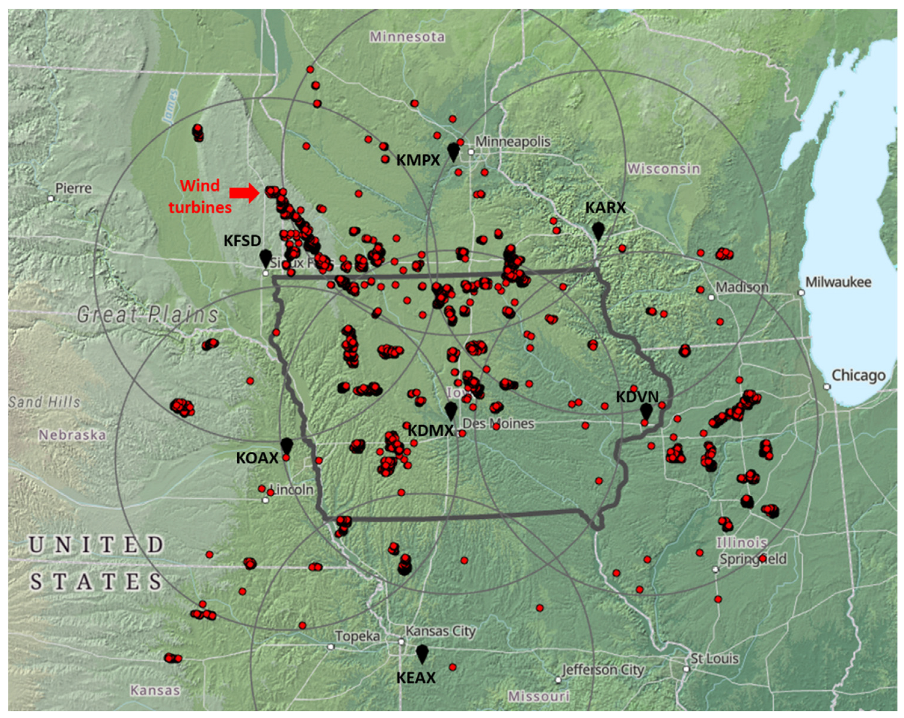
We developed new P/NP classification methods for WSR-88D radars and applied them to data collected from seven radars covering the state of Iowa, where the IFC conducts extensive research as well as operational activities, including weather monitoring and flood forecasting [18,19]. As shown in Figure 2, Iowa is covered by seven WSR-88D radars: KDMX (Des Moines, IA, USA), KDVN (Davenport, IA, USA), KFSD (Sioux Falls, SD, USA), KOAX (Omaha, NE, USA), KARX (La Crosse, WI, USA), KMPX (Minneapolis, MN, USA), and KEAX (Kansas City, MO, USA).
For model development, validation, and testing, we used data from the KDMX radar, which covers the majority of Iowa and most of its wind turbine locations, for the period from April through October 2017. Additionally, we collected data from all seven radars for model evaluation against rain gauge observations during April–October 2018.
The two primary input datasets used in this study are Level II data from WSR-88D radars and the Cloud and Moisture Imagery (CMI) products from the GOES-16 Advanced Baseline Imager (ABI). Both datasets are publicly available via cloud platforms (Amazon Web Services, Google Cloud) and the National Centers for Environmental Information (NCEI) archive [20]. Further details are provided below.

2.1.1. Radar Data

The Level II data from WSR-88D radars include three dual-polarimetric variables—differential reflectivity ( Z D R ), differential phase ( Φ D P ) and correlation coefficient ( ρ H V )—alongside conventional Doppler radar variables such as horizontal reflectivity ( Z h ), Doppler velocity ( V ), and spectrum width ( W ). Individual radar volume scans are produced every 4 to 10 min, depending on the Volume Coverage Pattern (VCP) used. The base scan (i.e., lowest elevation scan) provides a 0.5° azimuthal resolution and a 250 m gate spacing in range. In this study, we used all radar variables except the Doppler variables (V and W) for two primary reasons: (1) NP echoes from wind turbines may exhibit non-zero radial velocity, and (2) Doppler variables frequently have missing or invalid values in regions where the other variables are valid. We speculate that this issue arises from the use of the dual pulse repetition frequency (PRF) technique employed for velocity ambiguity mitigation [21,22]. Preliminary experiments also indicated that Doppler variables had limited importance relative to other radar features (note that Doppler variables are used at the signal processing stage for detection of stationary echoes).

2.1.2. GOES-16 Data

The ABI sensor onboard GOES-16 captures observations in 16 spectral bands, including six visible/near-infrared (VNIR) channels (0.5–1 km resolution) and ten infrared (IR) channels (2 km resolution). ABI operated in two primary scan modes. In Flex Mode, it performed full-disk scans every 15 min, CONUS (Continental U.S.) scans every 5 min, and mesoscale scans every 30 s. In contrast, Continuous Full-Disk Mode provided full-disk scans every 5 min [23]. Additional technical details on the ABI and its spectral properties are available in [23].
Among the Level 2+ products derived from ABI, we used the Cloud and Moisture Imagery (CMI) product from the CONUS scan, which offers near-real-time access and a temporal resolution (5 min) compatible with NEXRAD data. CMI products are expressed as dimensionless reflectance values for VNIR bands and as brightness temperatures (in degrees Kelvin) at the top of the atmosphere for IR bands. To avoid solar contamination of reflectance statistics, only IR channels were used in this study. These IR channels provide valuable information for characterizing surface and atmospheric features such as clouds, water vapor, ozone, volcanic ash, and dust.
For model efficiency, we selected five of the ten IR channels that are also employed in the GOES-R rainfall rate algorithm [17]: two water vapor bands (6.2 μm and 7.3 μm) and three IR window bands (8.4 μm, 11.2 μm, and 12.3 μm). Given the different temporal resolutions and unsynchronized measurement times of radar and satellite observations, radar and GOES-16 data were matched at each radar pixel using a nearest-neighbor approach in both space and time. Spatially, GOES-16 channel values were extracted from the satellite pixel nearest to each radar pixel center. Temporal collocation was performed by paring radar scan with the GOES-16 observation whose creation timestamp was nearest to the radar scan time. Although GOES-16 data may be redundant near the radar due to its coarser resolution (~2 km) than radar (250 m in range, 0.5° in azimuth), the complementary spatial resolutions are expected to enrich the feature set and increase diversity at the pixel level.

2.1.3. Rain Gauge Data

To evaluate the proposed model, we used rain gauge observations from two surface networks—the Automated Surface Observing System (ASOS) and the Automated Weather Observing System (AWOS)—available through the Iowa Environmental Mesonet (https://mesonet.agron.iastate.edu/ (accessed on 12 May 2025)). Both networks provide 1 min rainfall data, enabling straightforward aggregation into hourly totals that align with the radar accumulation interval. This minimizes missing values and ensures consistency across datasets.
In this study, we used hourly rain gauge data for hydrological evaluations to reduce uncertainties related to localized rainfall variability, measurement errors (in both radar and tipping buckets), gauge representativeness, and coordinate transformation [24].

2.1.4. IFC Radar Product

As a benchmark for model evaluation, we used the radar-rainfall products developed and operated by the IFC. These products are generated every five minutes from all seven NEXRAD radars covering Iowa and serve as the primary precipitation input for the IFC’s real-time flood forecasting system [18]. We accessed these datasets via the IFC-Cloud-NEXRAD system [25].
The system’s QPE algorithm (hereafter IFC algorithm) comprises several modules, including polarimetric-based quality control (e.g., removal of NP echoes [3]), hybrid scan product generation (e.g., CAPPI), multi-radar data integration, rainfall estimation using the NEXRAD Z-R relationship (e.g., Z = 300 R 1.4 ), and advection-corrected rainfall accumulation [26].

2.2. Methodology

2.2.1. Random Forest Classifier

The Random Forest classifier (hereafter RF), an ensemble of multiple independent decision trees, has gained widespread use due to several advantages: (1) strong predictive performance with efficient computation; (2) no assumption about the underlying data distribution; (3) capability to model nonlinear relationships between predictors and the response variable; (4) robustness to multicollinearity among features; (5) resilience to outliers and noise and overfitting; and (6) relatively simple model development with fewer tuning parameters (i.e., number of trees, nTree, and number of features considered at each node split, nTry) compared to other machine learning methods [13,14,15,27,28,29,30]. Although RF can be used for both classification and regression, it typically performs better in classification tasks, owing to the discrete nature of decision trees. In classification, predictions are determined by the majority class of samples assigned to a terminal node [30].
RF reduces classification error through ensemble averaging across decision trees. Each tree is constructed using a bootstrap sample (i.e., a random subset with replacement) from the training data and splits nodes using a random subset of nTry features to increase tree independence. The training and prediction process for RF is summarized as follows:
  • For each tree, two-thirds of the original samples (in-bag) are randomly selected for training. The remaining one-third (out-of-bag, OOB) samples are used for internal validation to estimate the model error (OOB score).
  • Trees grow to full depth using a splitting criterion known as Gini Gain, defined as the decrease in Gini Impurity (GI). At each node, a random subset of nTry predictors is evaluated, and the feature that maximizes the Gini Gain is used for splitting. GI is calculated as:
    G I = i = 1 C p ( i ) × ( 1 p i )
    where C is the number of classes, and p ( i ) is the proportion of samples belonging to class i . Gini Gain is the difference between the GI of the parent node and the weighted average GI of the child nodes, weighted by sample size. This continues until each terminal node contains samples of only one class.
  • Steps (1) and (2) are repeated until all n T r e e trees have been built.
  • Final predictions for unseen data are made via majority voting across all trees.
Two parameters are central to RF performance: n T r e e and n T r y . Higher n T r e e values can improve performance but with diminishing returns and higher computational cost. In contrast, n T r y has a greater impact on tree independence. A large n T r y increases the likelihood of dominant features being selected repeatedly, reducing tree independence. Conversely, a very small n T r y may increase error by overemphasizing weak predictors. In this study, we set n T r e e = 100 and n T r y = p , where p is the total number of input features. Preliminary analyses showed that increasing nTree beyond 100 had negligible benefits in accuracy (as measured by the OOB score), and p is a commonly recommended choice for classification tasks [27].

2.2.2. Training, Validation, and Test Sample Collection

As a supervised learning method, the RF classifier requires labeled training samples comprising input features and associated class labels (P or NP). Since this is a binary classification problem, both inter-class (P vs. NP) and intra-class (within P or NP) variability must be considered.
Precipitation can broadly be classified into convective and stratiform regimes, which are driven by distinct physical processes and exhibit different observational characteristics [16]. Convective precipitation is marked by strong vertical motions, high spatial variability, and intense rainfall, while stratiform precipitation is generally widespread, uniform, and weaker in intensity [16,31,32,33]. These regimes also have seasonal patterns: convective precipitation is more frequent in summer, whereas stratiform dominates in spring and fall in mid-latitudes. Thus, P samples must capture this seasonal behavior.
NP echoes, originating from diverse sources such as ground clutter, biological targets, and wind turbines, also exhibit different radar signatures. Ground clutter tends to produce noisy, random radar variables and near-zero radial velocities, while biological targets and wind turbines show non-zero Doppler velocities due to movement or rotation.
To capture this diversity, we collected Level II radar volume scans across different times of day and seasons. A key challenge was the lack of reference precipitation observations matching the spatial and temporal resolutions of NEXRAD data (e.g., 4–6 min in precipitation mode). To address this, we manually created P/NP mask maps for clearly distinguishable cases, where each mask was defined as a polygon, and all radar pixels at a single elevation scan within the polygon were taken as corresponding samples. To minimize artificial edge effects introduced by these polygon boundaries—which can distort local variability compared to the observed spatial variability of radar signals—we first computed local variability of radar observables before sampling within the masks. This approach ensured that the selected samples better represented the observed spatial variability of radar signals. All analyses were conducted in native radar coordinates (i.e., polar coordinates), focusing on single elevation scans—particularly the lowest scan—facilitating integration with single-scan radar QPE algorithms (e.g., those based on specific differential phase or attenuation) and avoiding reliance on vertical profiles, such as those used in the IFC algorithm (see Section 3.3).
Using this method, we collected 474 Level II volume scans from the KDMX radar between April and October 2017, totaling 56,291,370 samples. NP samples were more frequent, constituting 78% of the dataset. We split the samples into training/validation (75%, 42,278,528 samples) and testing (25%, 14,072,842 samples) sets. Two-thirds of the training/validation set (i.e., 28,185,685 samples) were used for model training, and one-third (i.e., 14,092,843 samples) were used as OOB samples for model validation. To minimize sampling bias in accuracy statistics, we intentionally designed the experiments so that OOB and test sets were similar in size. After model evaluation, the entire dataset was used to retrain the final model.

2.2.3. Model Evaluation Metrics

RF inherently performs internal cross-validation via OOB samples, and the average prediction accuracy for these samples is called the OOB score. Since OOB samples are not used in training individual trees, the OOB score provides an unbiased estimate of the model’s generalization performance [27,34]. It is calculated as:
O O B s c o r e = 1 n O O B i = 1 n O O B I ( Y ^ X O O B , i = Y O O B , i )
where I ( · ) is an indicator function (1 if true, 0 otherwise), Y ^ X O O B ,   i is the predicted label from majority voting among trees for which sample i was out-of-bag, X O O B ,   i is input features for sample i, and Y O O B , i the true label. n O O B is the total number of the OOB samples. This procedure eliminates the need for a separate validation set. Our experiments showed that the OOB score closely matches test set accuracy (Section 3.2).
To evaluate the model on independent test data and compare it with the IFC algorithm, we used the Probability of Detection (POD), False Alarm Ratio (FAR), and Heidke Skill Score (HSS), computed as:
P O D = a a + b
F A R = c a + c
H S S = 2 ( a d b c ) a + c c + d + ( a + b ) ( b + d )
where a = hits, b = false alarms, c = misses, and d = correct nulls (Table 1). POD measures the fraction of correctly identified NP cases, while FAR quantifies the rate of false NP predictions. HSS, also known as kappa [35], accounts for chance agreement and measures the model’s skill relative to random classification [36]. HSS ranges from –1 to 1, with negative values indicating performance worse than random, 0 indicating random-level performance, and 1 indicating perfect classification. Importantly, while POD and FAR are affected by which class is considered the target, HSS is class-invariant.

3. Results and Discussion

3.1. Single Feature Characteristics

Compared to NP echoes, P echoes typically exhibit higher copolar correlation coefficient values ( ρ H V > 0.9). For differential reflectivity ( Z D R ), values can vary due to raindrop ellipticity, but Z D R for P echoes generally remains lower relative to NP echoes. While P echoes often display a wide range of reflectivity ( Z ) and differential phase ( Φ D P ) values, Z also tends to be higher than that of NP echoes, which are typically around or below 20 dBZ, although exceptions such as ground clutter and anomalous propagation can exceed this value [1,3,37,38].
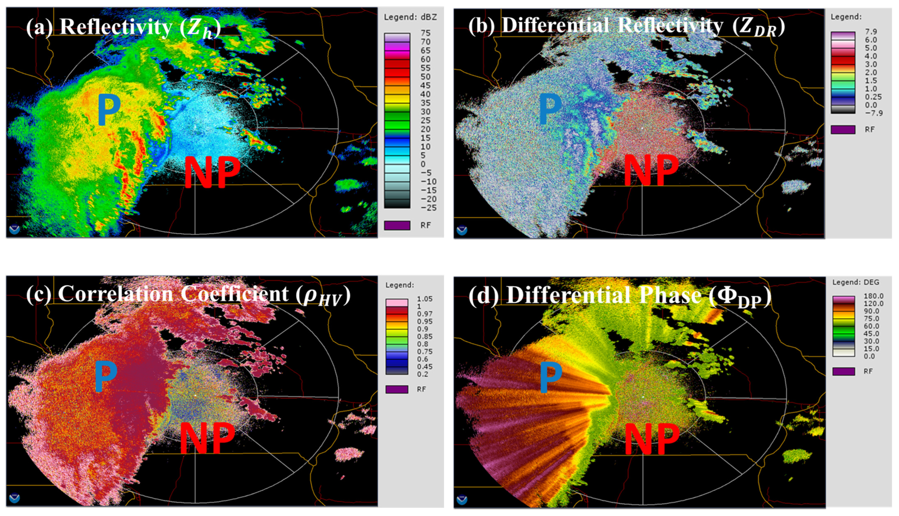
These differences between P and NP echoes can often be identified visually. For example, Figure 3 shows base scan maps (i.e., the lowest elevation scan) of various radar variables ( Z h , Z D R , Φ D P , and ρ H V ) measured by the KDMX radar at 07:59:41 UTC on 11 June 2015. The precipitation and non-precipitation areas are annotated with blue “P” and red “NP” labels, respectively. As shown, P echoes generally display higher ρ H V values (e.g., >0.85) and smaller Z D R values (e.g., <2 dB) compared to NP echoes. In addition to differences in magnitude, P echoes exhibit smoother spatial distributions. This spatial coherence results from the correlated nature of precipitation, whereas NP targets (e.g., birds, insects, ground clutter) produce more spatially incoherent radar returns. Based on these observations, one might attempt to remove NP echoes by applying appropriate threshold values to each variable. However, a key challenge lies in generalizing these thresholds so they remain effective under varying environmental conditions.
We analyzed the characteristics of radar variables and their local variability for both P and NP echoes using the collected sample dataset. Although no single variable alone is sufficient to fully distinguish between P and NP echoes, these distributions provide quantitative insight into how dual-polarimetric variables measured by S-band radars respond to different targets. As mentioned earlier, our proposed method is designed to rely solely on basic Level II radar variables and simple statistical measures such as local variance (or standard deviation), which enhances its applicability.
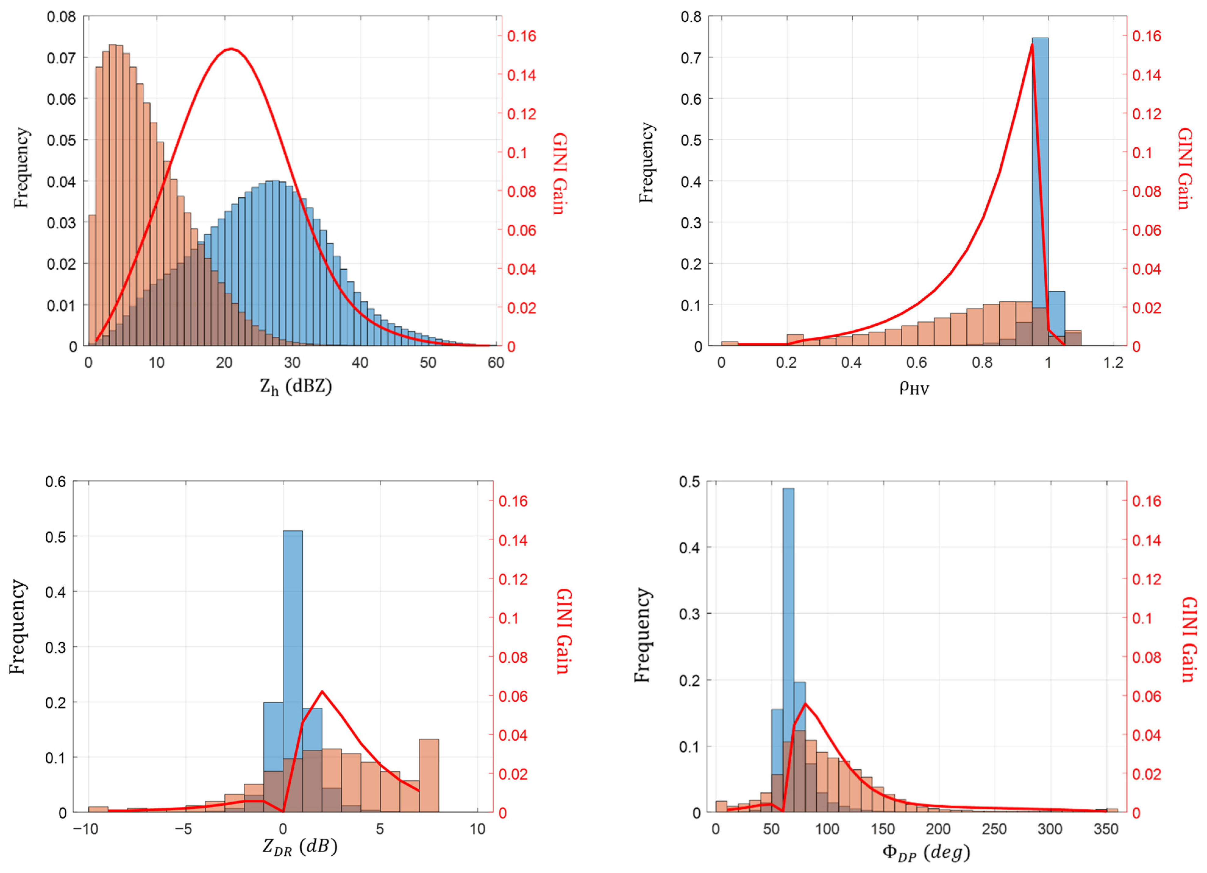
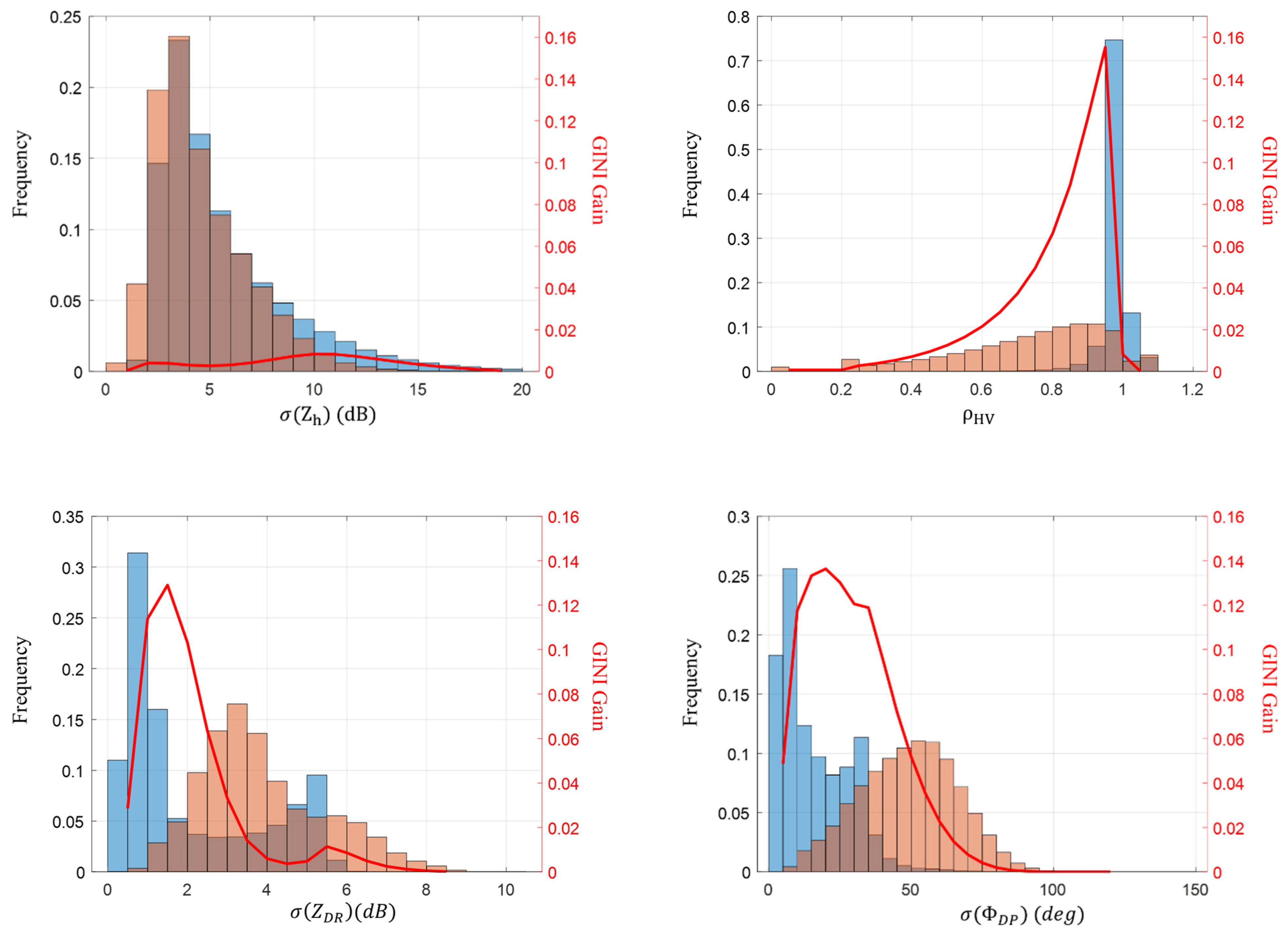
Figure 4 and Figure 5 present histograms of the radar variables (excluding Doppler variables) and their local variability, defined as the local standard deviation within a 13 × 13 pixel window (approximately 6.5° × 3.25 km) centered on the target pixel. Summary statistics for these distributions are provided in Table 2. Key findings are as follows:
  • Reflectivity ( Z h   ) values for NP echoes are generally lower than those for P echoes, with median values of 7.5 dBZ and 25.5 dBZ, respectively. Although the local variabilities of reflectivity do not differ significantly in magnitude (median: 3.80 dBZ for P and 3.84 dBZ for NP), this is primarily due to the lower absolute reflectivity values of NP echoes. The broader intensity range of P results in a wider interquartile range (IQR: 14.0 dBZ for P vs. 8.5 dBZ for NP).
  • The physical characteristics (e.g., shape, size, phase) of hydrometeors within a radar sampling volume are more consistent than those of NP targets. This consistency leads to smaller variations in both the amplitude and phase of the returned signal between the two polarimetric channels. Consequently, P echoes tend to exhibit higher ρ H V (indicating high correlation between polarimetric channels), and lower Z D R (indicating near-spherical particles).
  • In contrast, the randomness in magnitude and spatial distribution of NP echoes increases the local variability of dual-polarimetric variables ( ρ H V , Z D R , Φ D P ), resulting in broader distributions and higher standard deviations. All dual-polarimetric variables and their local variabilities exhibit lower IQRs and standard deviations for P echoes compared to NP echoes.
  • Some samples show relatively high local variability in ρ H V and Z D R . We attribute this to radar observations influenced by melting layers and echo boundaries between P and NP regions. The melting layer often contains a mix of melting snow, aggregates, graupel, or hail [1], and radar signals intersecting this region tend to reflect from a diverse mixture of hydrometeor types. This heterogeneity may cause decreases in ρ H V and increases in both Z D R and their respective local variabilities [39]. In this study, we treated radar observations affected by melting layers as P echoes. This classification is appropriate under the physical definition of precipitation, and such echoes should be retained during NP echo removal. However, quantifying the impact of melting layers on QPE accuracy lies beyond the scope of this study. Additional correction methods—such as melting layer (bright band) detection or vertical profile of reflectivity (VPR) corrections—should be considered to mitigate these effects.

3.2. Effects of Local Variabilities at Multiple Spatial Scales on Model Performances

We observed that the local variability of radar variables serves as a valuable discriminator for separating P and NP echoes. In this section, we evaluate the impact of various spatial scales used in calculating regional variability on the model’s classification accuracy.
Selecting an appropriate spatial scale for the local variability computation, which is defined by a specific window size, is a practical concern. The optimal scale should maximize the statistical distinction in local variability estimates between P and NP echoes. Specifically, the scale (i.e., window size) must be large enough to effectively capture the randomized spatial structure typical of NP echoes, while remaining small enough to reflect the relatively smooth horizontal variability of small-scale convective storms. To identify the best-performing spatial scales, we analyzed the effect of different window sizes on out-of-bag (OOB) scores from the random forest classifier.
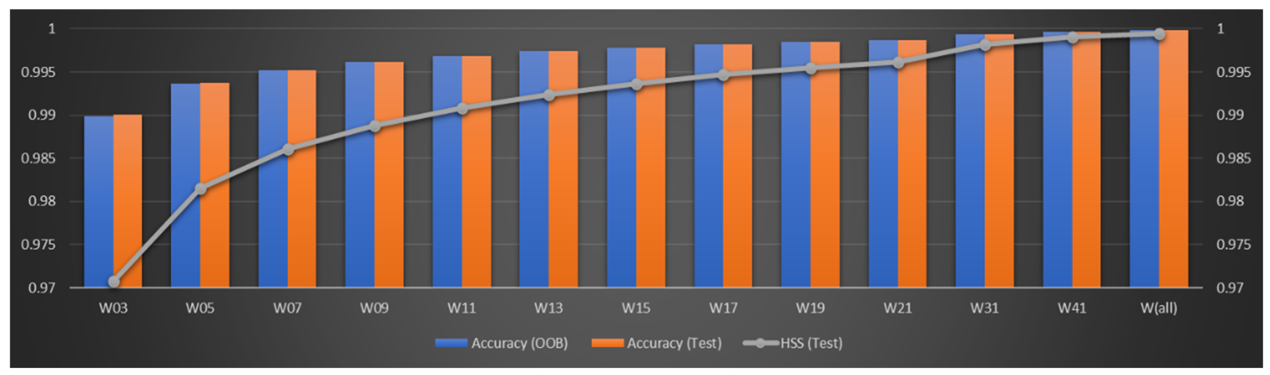
Figure 6 shows a monotonically increasing trend in classification accuracy (OOB score) as the window size increases. The overall accuracy of models using window sizes ranging from 3 × 3 (w03) to 41 × 41 (w41) improved from 0.9899 to 0.9997. The selection of the maximum window size (i.e., 41 × 41) is arbitrary, but this converging pattern suggests that further increases beyond a 41 × 41 window size would result in only marginal accuracy gains. Notably, model accuracies on the test samples are nearly identical to the OOB scores, experimentally confirming the OOB score’s unbiased nature. The Heidke Skill Score (HSS) also increased monotonically, from 0.9708 (w03) to 0.9990 (w41), demonstrating that the presence of imbalanced class distributions (P vs. NP) did not influence the selection of an appropriate window size. HSS is particularly useful in this context as it quantifies classification skill while accounting for class imbalance.
Smaller window sizes (e.g., 5 × 5) tend to preserve weak echoes located at the edges of storms. In contrast, models using larger window sizes are more likely to classify such weak signals as NP echoes. This is likely due to the fact that larger windows yield higher local variability estimates at the edges, which reduce the contrast between P and NP echoes. On the other hand, larger window sizes (e.g., 41 × 41) are more effective at removing NP echoes caused by wind turbines, which often produce spatially coherent radar signatures similar to those of P. The extent of this contamination varies depending on the coverage and distribution of wind farms within the radar domain.
To leverage the advantages offered by the characteristics of local variability estimates at multiple scales, we elected to use all of them as features for the main RF model. This approach enables the model to incorporate scale-dependent variability in P signatures. As shown in Figure 6, the OOB score, test set classification accuracy, and HSS for the final composite model [W(all)] are 0.9998, 0.9998, and 0.9995, respectively, representing the highest performance among all tested configurations.

3.3. Performance Assessment Against the IFC Algorithm

The main model incorporated radar variables ( Z , Z D R , ρ H V , and Φ D P ) along with their local variability estimates—specifically, standard deviations calculated within neighboring pixels across 12 window sizes, as shown in Figure 6. Based on evaluation with the test dataset, the model achieves a classification accuracy of 0.9998 and a HSS of 0.9995 for distinguishing between P and NP echoes. In this section, we assess the proposed model’s performance relative to the IFC system. Specifically, we examine (1) the effectiveness of the model in addressing limitations inherent in heuristic, rule-based approaches, and (2) the consistency of classification accuracy across different range intervals (i.e., distances from the radar).
Due to the radar measurement strategy, beam geometry and sampling volume vary with range. Near the radar, observations are more susceptible to side-lobe effects and ground clutter. These issues are typically mitigated by radar signal processing systems before the Level II data products are generated. At farther ranges, however, phenomena such as beam overshooting, broadening, and loss of sensitivity can degrade radar data quality. These factors can alter the statistical characteristics of radar variables for both P and NP echoes and are often influenced by environmental conditions.
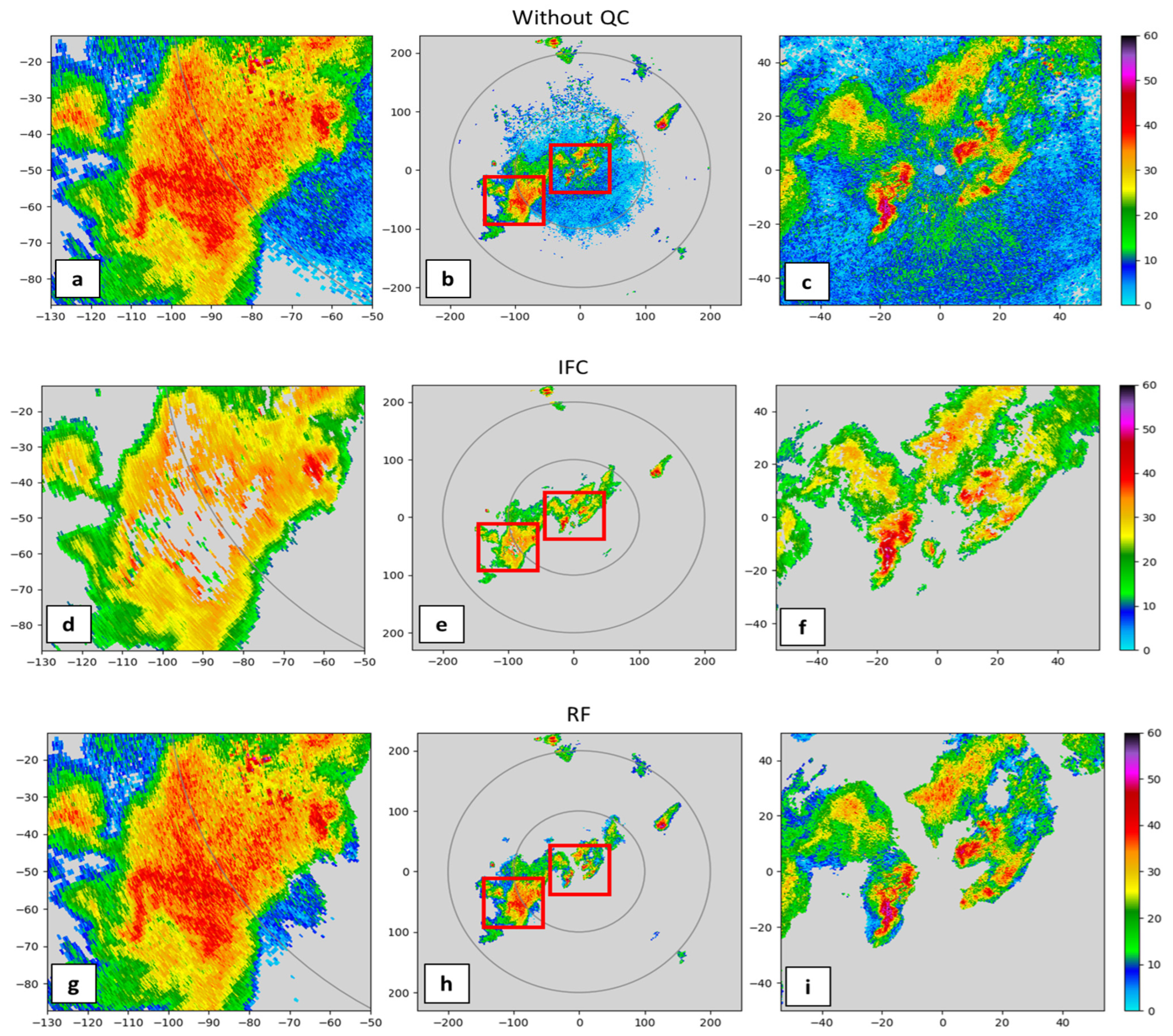
Rule-based algorithms, such as those used in the IFC system [3], can struggle under such variable conditions, largely due to their reliance on fixed threshold values. Figure 7 illustrates reflectivity maps with and without NP echo removal using the IFC algorithm (panels d–f) and the proposed main RF model (panels g–i). The raw radar data were acquired by the KDMX radar at 02:48:02 UTC on 1 July 2017, and contain embedded NP echoes within a precipitation field.
Both the IFC and main RF models successfully remove most NP echoes. However, the IFC model shows false NP echo removal near the radar, manifested as small, randomly distributed holes in the reflectivity field (Figure 7f). We speculate that while most return signals originate from precipitation, residual ground clutter may alter the statistical features of the radar variables. When the contaminated values approach the fixed thresholds used by the heuristic model, misclassification may occur. The location of such errors is difficult to determine due to the random nature of contamination. Additionally, Figure 7d shows a larger area of erroneous NP classification, coinciding with a known wind turbine cluster. Although the IFC algorithm is designed to remove wind turbine interference, the result suggests an overcorrection in this case.
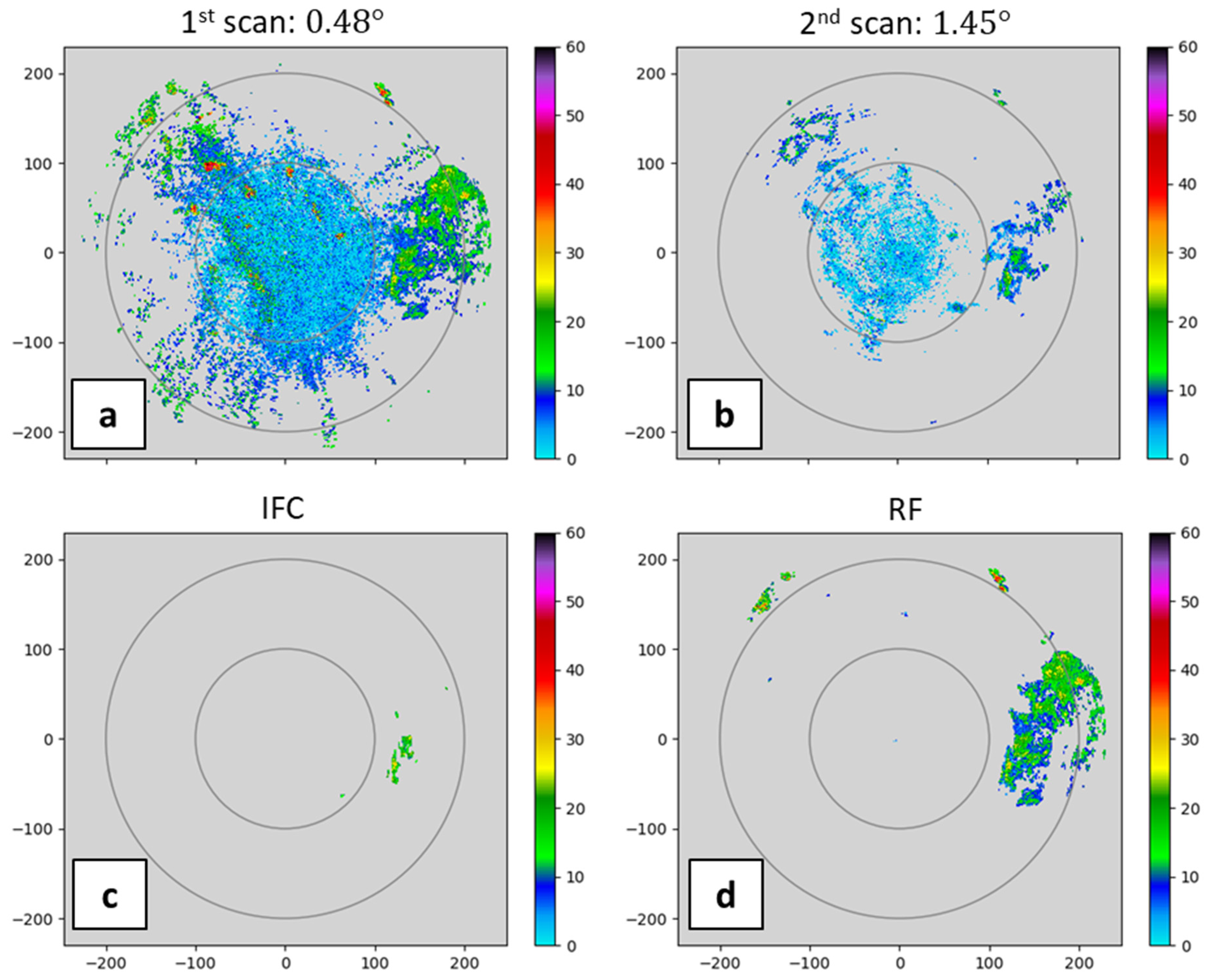
Figure 8 presents a case of beam overshooting, observed at 07:21:07 UTC on 1 July 2017. This scenario highlights another limitation of the IFC algorithm. One of its key components involves estimating the vertical reflectivity gradient, following the method proposed by [40], to identify anomalous propagation (AP) conditions. While this method preserves the three-dimensional structure of radar observations—facilitating applications such as hybrid scan construction and vertical profile simulations—it can lead to incorrect NP classification when beams at higher elevation angles (e.g., the second elevation scan) overshoot precipitation. In such cases, the negative reflectivity gradient is misinterpreted as an AP signal. Moreover, this gradient-based method is sensitive to changes in VCP modes [41,42], which alter both the number and elevation angles of radar scans. For example, VCP 12 consists of 14 scans at 17 elevation angles, whereas VCP 221 includes only 11 scans at 9 angles [41,42], making a universally applicable threshold difficult to define.
Compared to the IFC algorithm, Figure 7g–i and Figure 8d demonstrate the superior performance of the new main RF model in retaining valid P echoes while effectively eliminating NP echoes, even in challenging cases. To further assess the model’s general performance across varying conditions, we applied it to test data segmented into three range zones: Zone 1 (0–75 km), Zone 2 (75–150 km), and Zone 3 (150–230 km). Table 3 summarizes the results using POD, FAR, and HSS. Here, POD and FAR measure the detection skill for NP echoes, while HSS reflects overall classification skill, integrating both P and NP detection performance.
Both the IFC and RF models perform well in removing NP echoes across all ranges (POD > 0.99). However, the ability of the IFC algorithm to retain P echoes decreases significantly with range. Specifically, its FAR increases from 0.0169 in Zone 1 to 0.1339 in Zone 2, and further to 0.7705 in Zone 3. In contrast, the RF model maintains a consistently low FAR across all zones (0.0001–0.0041), indicating robust performance even at extended distances. These improvements are reflected in the consistently high HSS values, confirming the model’s effectiveness in both NP removal and P echo retention across all ranges.
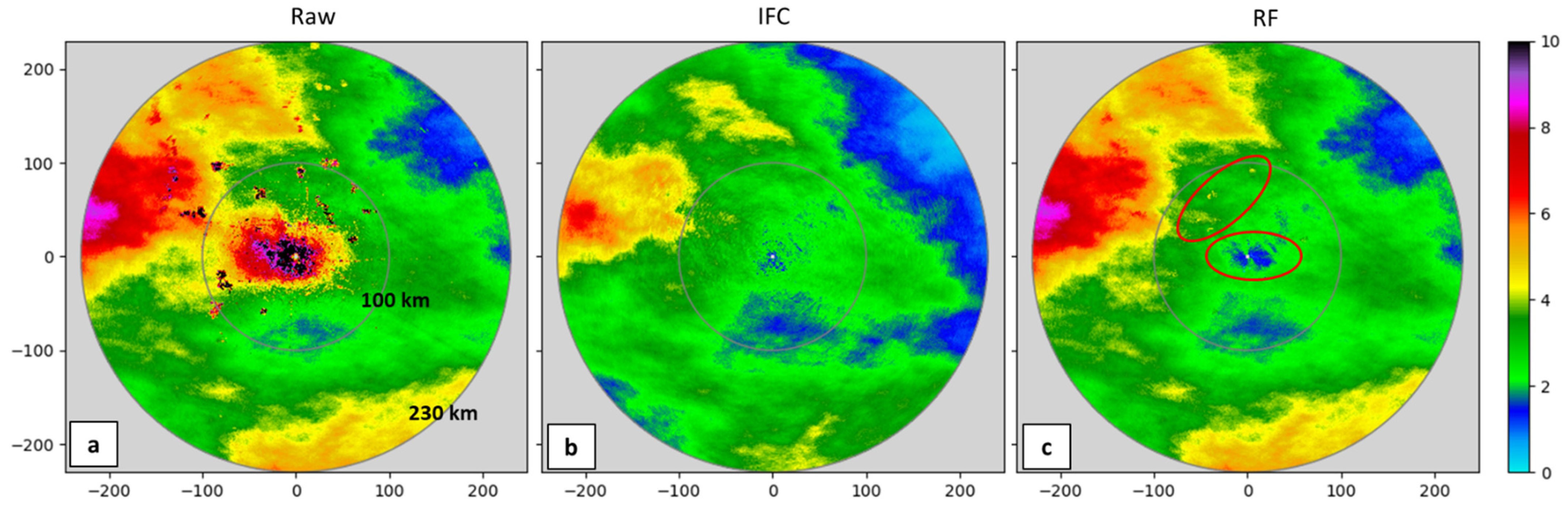
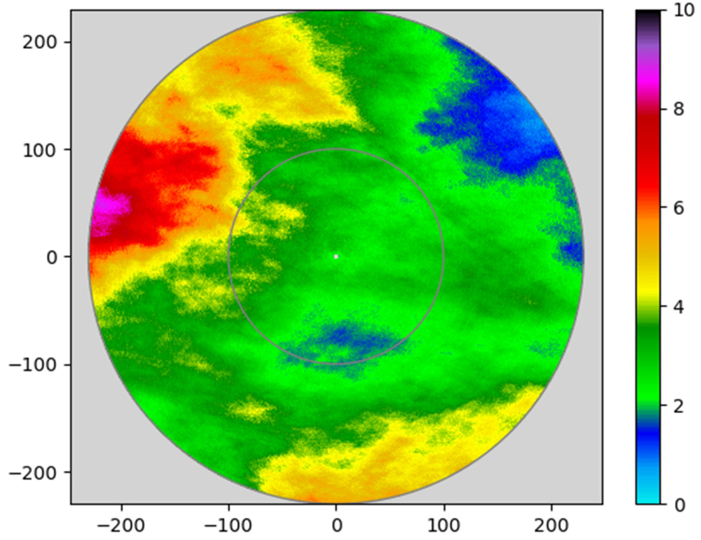
To evaluate model performance over time, we also computed maps of the Probability of Rainfall Detection (PORD) for raw reflectivity data and after applying the IFC and RF models (Figure 9). PORD is defined as the percentage of observations exceeding a reflectivity threshold. Using all KDMX Level II data from August 2017, we applied a threshold of 20 dBZ, corresponding to a rainfall rate of 0.46 mm/h based on the WSR-88D convective Z–R relationship ( Z = 300 R 1.4 ). Both models effectively eliminate abnormally high PORD values near the radar and wind turbine clusters. However, the IFC algorithm tends to remove P echoes as NP at farther distances. In contrast, the RF model preserves the spatial structure of P echoes at far ranges, consistent with the raw data. This is attributable to the RF model’s reliance on polarimetric signatures and their spatial variability, which supports its applicability out to 230 km—the typical range for dual-polarimetric radar measurements.

3.4. Supplementary Model with GOES 16 Data

The proposed RF model (i.e., the main model) demonstrates strong classification performance in distinguishing between P and NP echoes. We explore further enhancements using an independent data source in this section—GOES-16 infrared products—and a multi-layer scanning approach based on the Constant Altitude Plan Position Indicator (CAPPI) method in the following section.
In certain cases, polarimetric radar signatures from wind turbine clusters are nearly indistinguishable from those of P echoes (e.g., the red-circled region in the upper-left of Figure 9c). These echoes may exhibit smooth spatial distributions in radar variables, along with elevated Z and ρ H V values.
To address this issue, we trained a supplementary RF model incorporating GOES-16 products. Training samples were collected from July to October 2017, using the P and NP masks described earlier. As detailed in Section 2.2.1, this supplementary model utilizes brightness temperature data from five GOES-16 infrared channels, along with the four radar variables at the corresponding sample points (see Section 2.1.2).
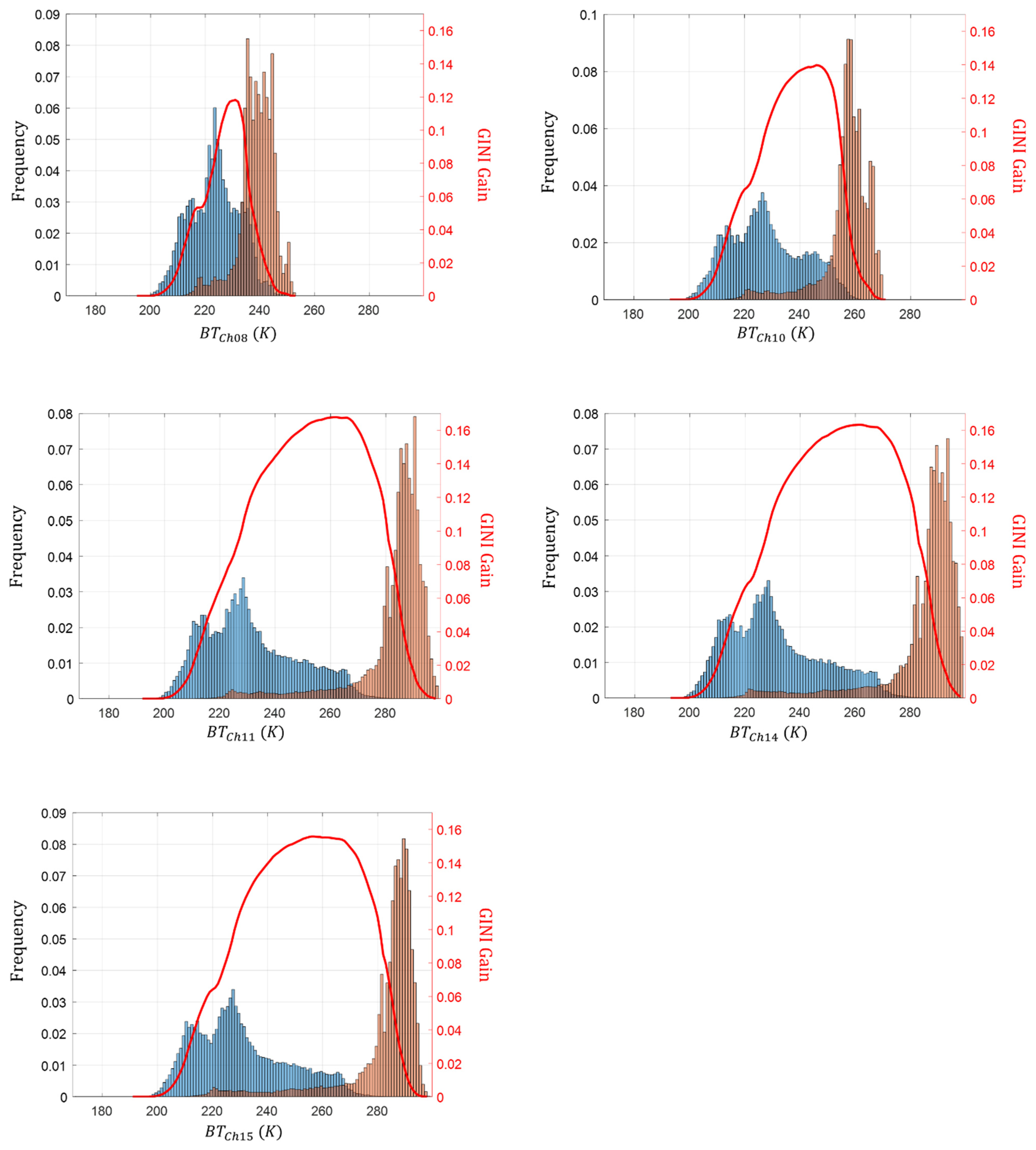
Figure 10 presents histograms of brightness temperatures (in degree Kelvin) across the five selected GOES-16 channels. As expected, P echoes exhibit lower brightness temperatures than NP echoes, due to increased absorption of Earth-emitted infrared radiation by precipitation [23]. This characteristic provides a useful discriminator, enabling the supplementary model to refine the classification further—specifically, by reclassifying NP echoes that the main RF model initially misclassified as P (RF-GOES, Figure 11).

3.5. Further Improvement with CAPPI Scan Strategy

Another challenge arises from radar measurement contamination in areas close to the radar (e.g., within ~20 km), where the radar sampling volume is small (e.g., less than 200 m in azimuth at 20 km for a 0.5° beamwidth). In such regions, radar measurements are more susceptible to ground clutter contamination (e.g., the red-circled area centered in Figure 9c). As previously discussed, the radar signal processing system may alter return signal characteristics during ground clutter suppression, potentially compromising measurement accuracy.
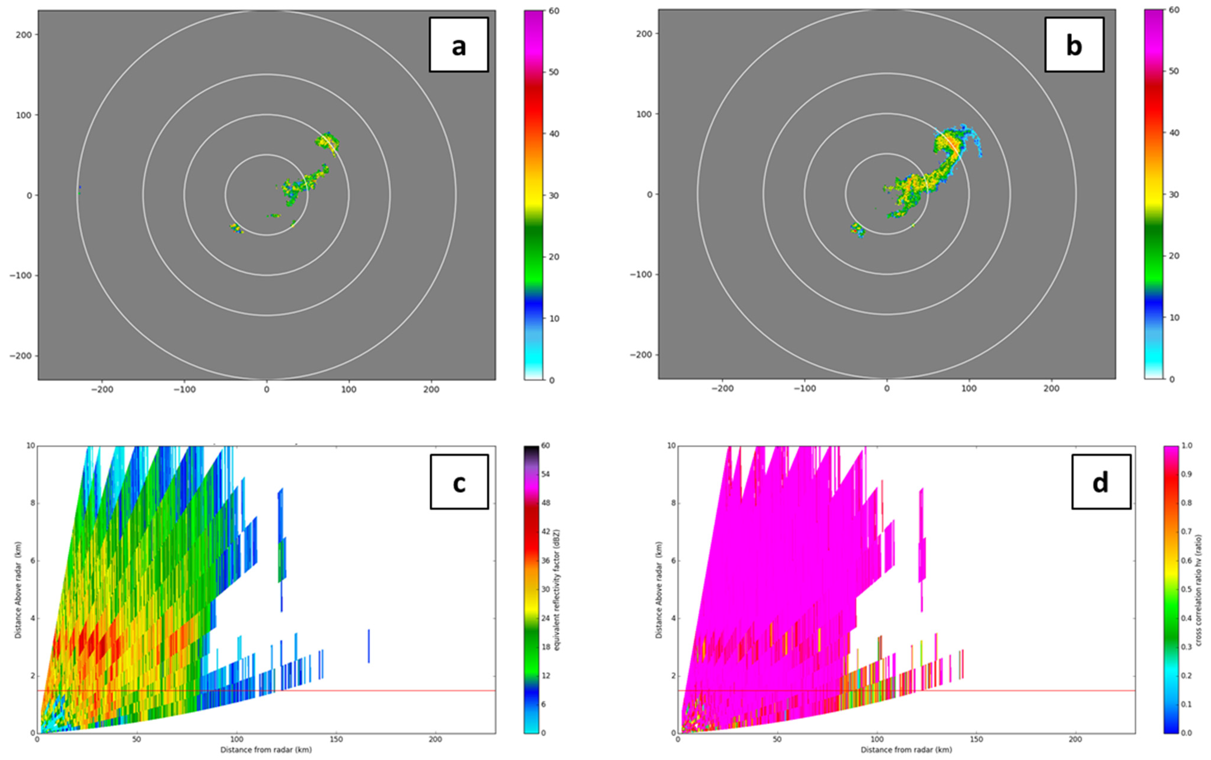
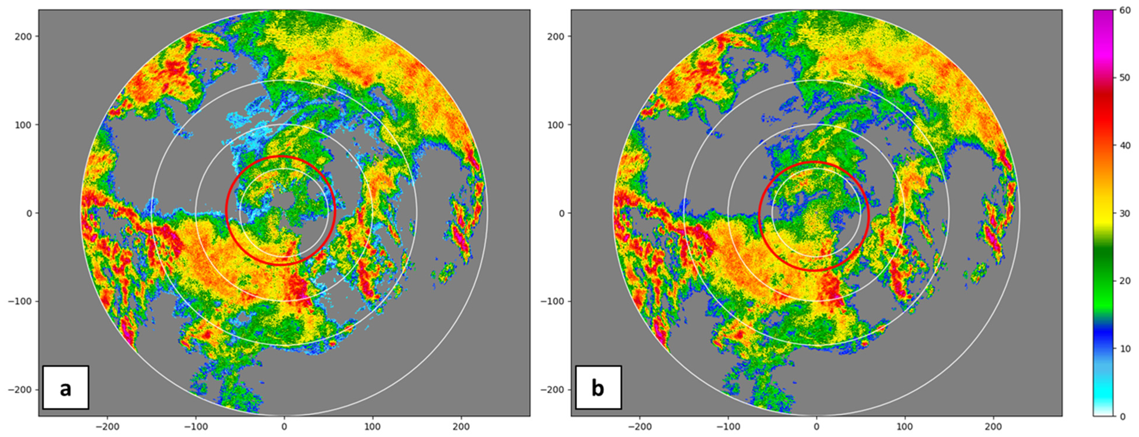
Figure 12 illustrates this effect: at 1.32° (third elevation scan), the radar detects a broader area of precipitation around the radar than at the lowest elevation scan (0.48°). The vertical profiles of reflectivity (Figure 12c) and ρ H V (Figure 12d) along the 70° azimuth further highlight this discrepancy. At the lowest elevation, weak Z and low ρ H V , coupled with high variability, make it difficult to confirm the presence of precipitation. To mitigate this issue, we propose leveraging higher elevation scans in the near-radar region using the CAPPI scan strategy used in the IFC algorithm to avoid overly sensitive or distorted measurements at the lowest elevation. In this method, RF-GOES method is applied to all volume scans, and the filtered reflectivity data is remapped onto a fixed polar grid with 0.25 km range and 0.5° azimuthal resolution. A log-normal kernel was then applied to vertically interpolate reflectivity values across elevation angles, assigning normalized weights based on proximity to a specified CAPPI height [26]. For a demonstration purpose, we used 1.5 km altitude as the CAPPI height in this study (RF-GOES CAPPI), but the optimal height would vary depending on the climatology for an area of interest. Applying a CAPPI scan strategy allowed us to fill in the reflectivity “hole” near the radar while preserving the magnitude and spatial structure of the surrounding reflectivity field (Figure 13). As a result, we observed that combining the main and supplementary RF models, together with the CAPPI scan strategy, led to improved classification performance (Figure 14). In this process, we generated CAPPI maps by (1) applying the established models to individual elevation scans and (2) merging the two filtered reflectivity fields closest to the target altitude (1.5 km) using an inverse-distance weighted interpolation method.

3.6. Discussion on the Accuracy Improvements

This section evaluates the individual contributions of the three proposed methods: (1) the main RF model employing multi-scale polarimetric features (RF), (2) the integration of GOES-16 satellite data (RF-GOES), constructed by sequentially applying the main RF model followed by a supplementary GOES-16-based model, and (3) the Constant Altitude Plan Position Indicator (CAPPI) scan strategy applied to the RF-GOES outputs from all elevation scans (RF-GOES CAPPI). Due to the lack of collocated ground truth in regions affected by localized contamination, performance is assessed qualitatively using spatial derivatives of PORD, as introduced earlier (e.g., Figure 9, Figure 11 and Figure 14), which reflect the spatial consistency and physical plausibility of classified precipitation fields.
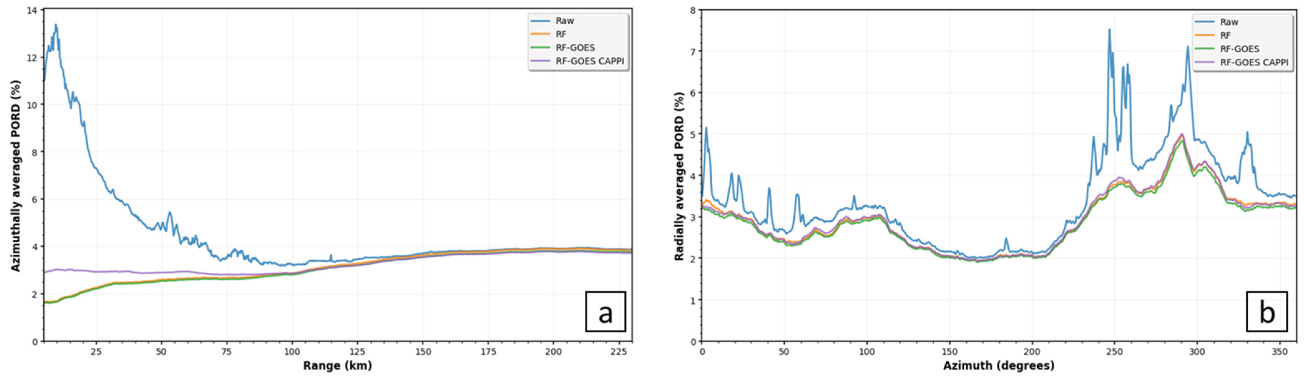
Figure 15a and Table 4 present the azimuthally averaged PORD as a function of range. The raw Level II reflectivity exhibits anomalously high PORD values near the radar (maximum: 13.38% at 9.62 km) and substantial radial variability in the derivatives (standard deviation: 0.1442% in Zone 1), attributed to ground clutter. In contrast, the RF (PORD: 1.6991% at 9.62 km; STD: 0.0092%) and RF-GOES (PORD: 1.6604%; STD: 0.0088%) models, both relying solely on the lowest elevation scan, significantly reduce this variability. However, their lower PORD values near the radar, along with increasing trends with distance, suggest under-detection of precipitation in this region. The RF-GOES CAPPI model achieves the greatest reduction in variability and yields a more consistent radial profile (PORD: 3.03% at 9.62 km, STD: 0.0049%), indicating both effective suppression of NP echoes and improved recovery of valid precipitation near the radar.
To assess the impact of the GOES-16-based models (RF-GOES and RF-GOES CAPPI), we examine the azimuthal profile of radially averaged PORD between 75–125 km (Figure 15b), where wind turbine-induced NP echoes are prevalent. The raw data exhibit pronounced PORD spikes at azimuths corresponding to turbine locations, resulting in high azimuthal variability. The RF model reduces this variability by 84.65% (Table 4), while the RF-GOES and RF-GOES CAPPI models achieve slightly greater reductions (85.49% and 85.51%, respectively). These results, along with those in Section 3.3, suggest that the radar-only RF model is effective in removing most NP echoes. Nevertheless, the incremental benefit of incorporating satellite data remains valuable, particularly for suppressing localized NP artifacts that may exhibit high reflectivity. As expected, the RF-GOES CAPPI model has negligible additional impact in this region, where the lowest elevation scan dominates the CAPPI construction.
Table 4 summarizes the comparative performance of each model configuration. The main RF model provides a strong baseline through multi-scale polarimetric features. The GOES-16 products enhance the discrimination of NP echoes with precipitation-like signatures, particularly those associated with wind turbines. The CAPPI strategy significantly improves near-radar detection by mitigating under-detection caused by signal contamination. Each method contributes distinct value to the overall system performance. The integrated RF-GOES CAPPI model, which combines radar-based multi-scale features, satellite data, and CAPPI scan strategy, delivers the most consistent and physically realistic classification outcomes across a range of spatial contexts.

3.7. Hydrological Assessment

To objectively evaluate the model’s overall performance using independent data sources, in this section we compare hourly PORD values over the state of Iowa derived from the proposed models against reference datasets, including rain gauges, Multi-Radar Multi-Sensor (MRMS) products, and STAGE IV estimates. We used an hourly temporal scale to ensure fair comparisons, given the differing temporal resolutions across radar datasets. State-wide rainfall maps were generated using the IFC algorithm [25]. The verification period spans seven months, from April to October 2018. Corresponding MRMS radar-only, gauge-corrected, and STAGE IV hourly rainfall data were obtained from the IFC archives.
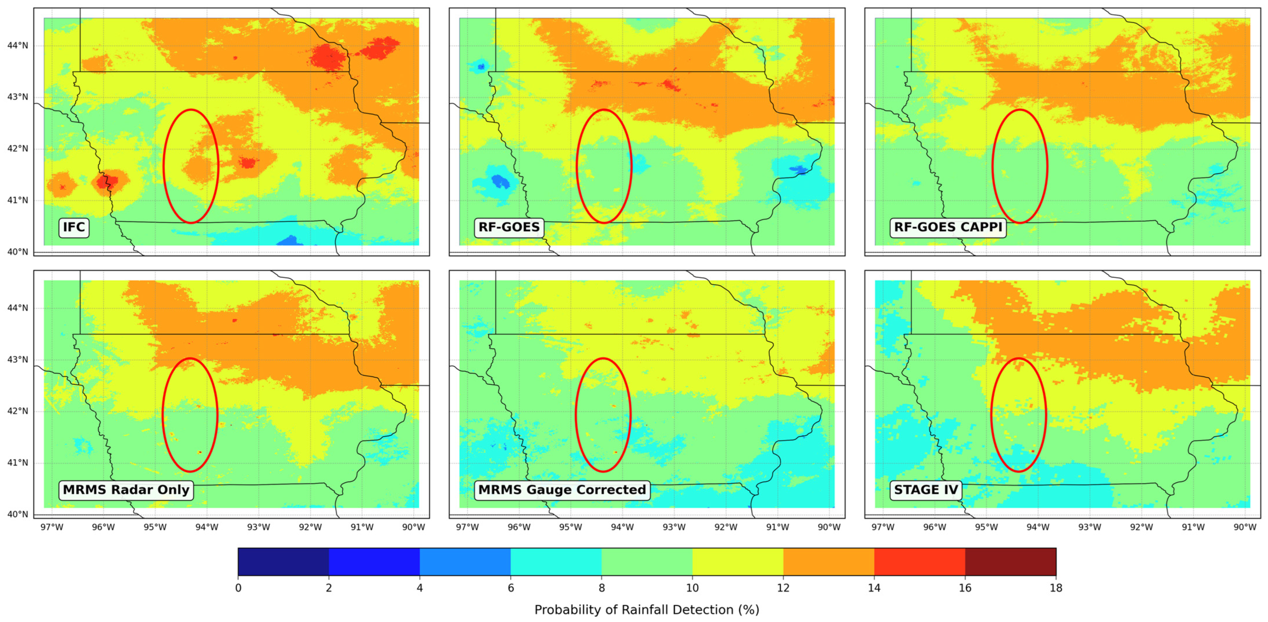
Since the true rainfall distribution at the ground level is not directly observable as mentioned in Section 3.6, we first conducted a qualitative comparison of the PORD values generated by the proposed models and those from other radar-based products (Figure 16). To isolate the influence of algorithmic differences on rainfall detection, we used a threshold of 0.254 mm/h, which corresponds to the minimum measurable amount by a standard tipping-bucket rain gauge.
As shown in Figure 16, the IFC algorithm tends to overestimate PORD values—indicating a higher frequency of rainfall detection—particularly in areas near radar sites. We attribute this tendency to limitations in the fixed threshold approach, which may fail to adapt to varying environmental conditions, as discussed previously. In contrast, the RF-GOES model effectively suppressed wind turbine-induced artifacts, as shown by the red-circled regions in Figure 16.
Both MRMS products (radar-only and gauge-corrected) and STAGE IV occasionally failed to eliminate wind turbine artifacts at certain locations. Although the hydrological impact of these residual echoes is likely minimal due to their limited spatial extent, the implications may vary depending on the severity of wind turbine interference (see [4]). Notably, the CAPPI scan strategy (RF-GOES CAPPI) further enhanced rainfall detection near radar sites while maintaining effective suppression of NP echoes.
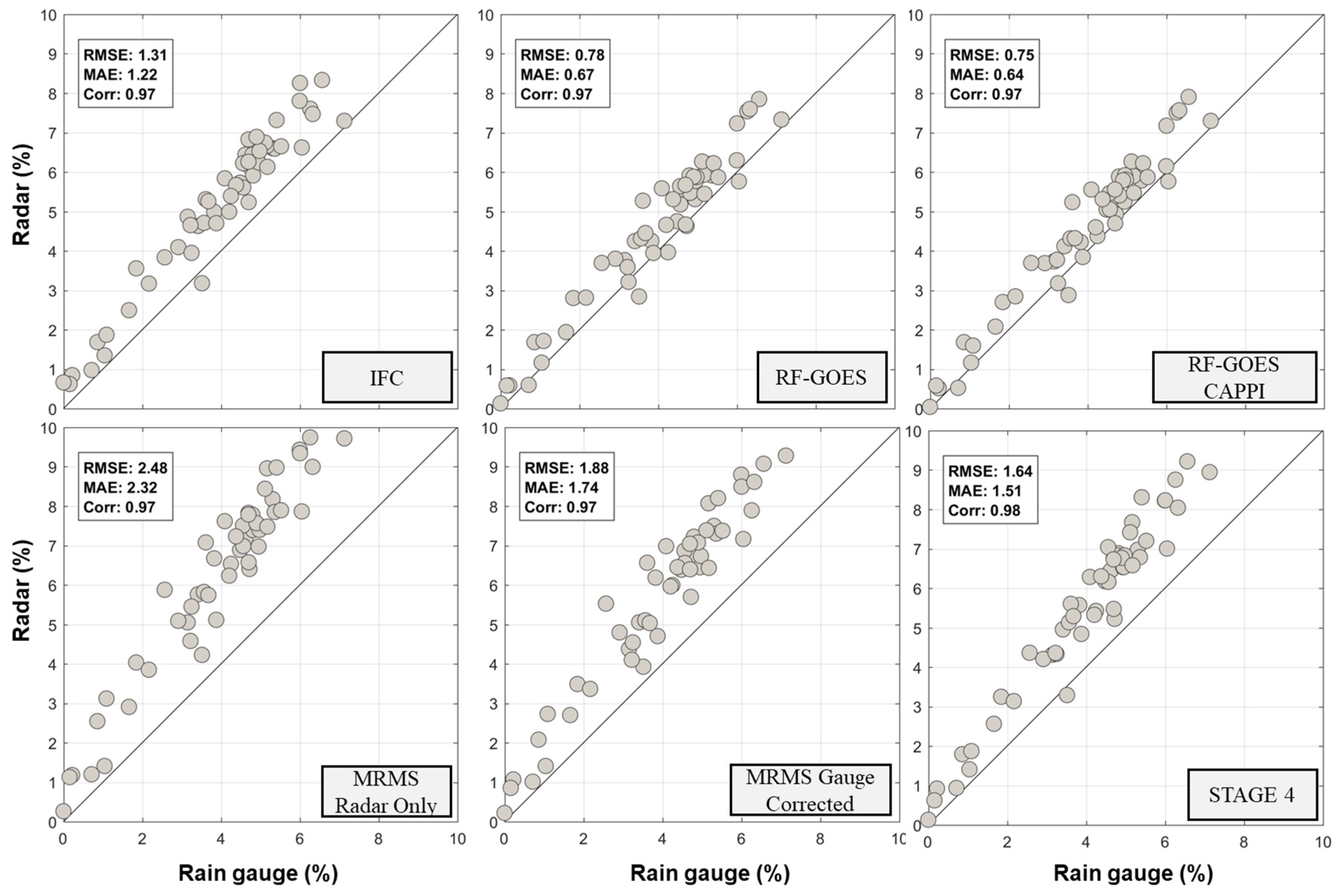
Finally, comparison with ground-based rain gauge observations in Figure 17 indicates that the CAPPI-based product exhibits the smallest PORD errors such as root mean square error (RMSE) and mean absolute error (MAE) among all evaluated datasets, providing additional evidence of the robustness and hydrological utility of the proposed model.

4. Summary and Conclusions

This study presents a robust, data-driven framework for the classification and removal of non-precipitation (NP) echoes from dual-polarimetric radar observations using a Random Forest (RF) classifier. The proposed model is designed for operational scalability, requiring minimal hyperparameter tuning while maintaining resilience to overfitting and observational noise. By leveraging multi-scale spatial variability in radar signatures, the main RF model achieved classification accuracy exceeding 99.98% on a large and diverse dataset comprising 474 Level II volume scans from the KDMX radar. This high performance was consistent across a wide range of environmental conditions, precipitation regimes, and distances from the radar, demonstrating the model’s generalizability and robustness.
Despite the strong performance of the model, two practical challenges were identified. First, NP echoes with precipitation-like signatures—such as those generated by wind turbines—can evade detection due to their high reflectivity and spatial coherence. Second, under-detection of precipitation near the radar often occurs due to signal contamination from side-lobe interference and aggressive ground clutter suppression, which distorts the lowest elevation scan. To address these limitations, we introduced two complementary enhancements: (1) the integration of GOES-16 infrared satellite products and (2) the application of a Constant Altitude Plan Position Indicator (CAPPI) scan strategy.
The GOES-16-based supplementary RF model applied to the residual of the main RF model (i.e., RF-GOES) improved the suppression of localized NP artefacts, particularly wind turbine clutter, by exploiting the brightness temperature differences at various channels between precipitation and non-meteorological targets. The CAPPI scan strategy, applied to the outputs of the RF-GOES model, significantly improved near-radar precipitation detection by incorporating higher-elevation scans to recover valid echoes misclassified as NP due to signal degradation near the radar at lowest elevation scan. The qualitative evaluations using the PORD and its spatial derivatives demonstrated that the RF-GOES CAPPI model reduced radial variability near the radar caused by NP echoes in raw reflectivity by over 96% and improved azimuthal consistency in regions affected by wind turbine interference. Hydrological validation against rain gauge observations and other operational QPE products further confirmed the model’s superiority, with the CAPPI-enhanced product yielding the lowest root mean square error (RMSE) and mean absolute error (MAE) among all evaluated datasets.
Note that this study relies on Level II dual-polarimetric radar data, which, while operationally practical, does not provide access to raw signal-level information. Advanced techniques for target characterization using the full polarimetric scattering matrix, such as general polarimetric correlation patterns [43] or multidomain joint-domain scattering analysis [44], could potentially enhance target discrimination, particularly in challenging cases such as wind turbine clutter or near-radar contamination. Additionally, while the proposed approach is designed for easy transferability of the development methodology, which relies on fundamental radar variables (e.g., reflectivity, differential reflectivity, correlation coefficient) and avoids complex preprocessing, its performance across different radar systems and geographic regions warrants further investigation.
Overall, the integrated RF-GOES-CAPPI framework offers a practical and effective solution for improving the quality of radar-based precipitation products. By combining radars’ multi-scale polarimetric features, satellite-derived brightness temperatures, and CAPPI scan strategy, the proposed method addresses key limitations of existing NP removal algorithms and supports more accurate and physically consistent rainfall estimation in operational hydrometeorological applications.

Author Contributions

Conceptualization, M.K., B.-C.S. and W.F.K.; methodology, M.K.; software, M.K. and B.-C.S.; validation, M.K.; formal analysis, M.K.; investigation, M.K.; data curation, M.K.; discussion on the results, all authors; writing—original draft preparation, M.K.; writing—review and editing, all authors; visualization, M.K.; supervision, W.F.K. All authors have read and agreed to the published version of the manuscript.

Funding

This work was supported by the Iowa Flood Center at the University of Iowa in Iowa, the United States. This work was also partially supported by the Global Joint Research Program funded by the Pukyong National University (Project number: 202412100001) in Busan, South Korea, and by the National Research Foundation of Korea (NRF) grant funded by the Korea government (MSIT)(RS-2025-00563294).

Data Availability Statement

All raw NEXRAD Level II radar data and NOAA Geostationary Operational Environmental Satellite (GOES-16) products used in this study are publicly accessible via Amazon Web Services (AWS) at https://registry.opendata.aws/noaa-nexrad/ (accessed on 12 May 2025) and GOES-16: https://registry.opendata.aws/noaa-goes/ (accessed on 12 May 2025), respectively. The processed data presented in this study are available on request from the corresponding author due to privacy. All original contributions presented in this study are included within the article. For further information or inquiries, please contact the corresponding authors.

Acknowledgments

During the preparation of this manuscript, the authors used ChatGPT-4o mini (OpenAI) for English editing purpose. The authors have reviewed and edited the output and take full responsibility for the content of this publication.

Conflicts of Interest

Author Munsung Keem was employed by the company Fundamental Data Science, Louis Dreyfus Company Asia Pte. Ltd. The remaining authors declare that the research was conducted in the absence of any commercial or financial relationships that could be construed as a potential conflict of interest.

References

  1. Tang, L.; Zhang, J.; Langston, C.; Krause, J.; Howard, K.; Lakshmanan, V. A Physically Based Precipitation–Nonprecipitation Radar Echo Classifier Using Polarimetric and Environmental Data in a Real-Time National System. Weather Forecast. 2014, 29, 1106–1119. [Google Scholar] [CrossRef] [Scilit]
  2. Islam, T.; Rico-Ramirez, M.A.; Han, D.; Srivastava, P.K. Artificial Intelligence Techniques for Clutter Identification with Polarimetric Radar Signatures. Atmos. Res. 2012, 109–110, 95–113. [Google Scholar] [CrossRef] [Scilit]
  3. Seo, B.-C.; Krajewski, W.F.; Mishra, K.V. Using the New Dual-Polarimetric Capability of WSR-88D to Eliminate Anomalous Propagation and Wind Turbine Effects in Radar-Rainfall. Atmos. Res. 2015, 153, 296–309. [Google Scholar] [CrossRef] [Scilit]
  4. Ghimire, G.R.; Krajewski, W.F. Hydrologic Implications of Wind Farm Effect on Radar-Rainfall Observations. Geophys. Res. Lett. 2020, 47, e2020GL089188. [Google Scholar] [CrossRef] [Scilit]
  5. Park, H.S.; Ryzhkov, A.V.; Zrnić, D.S.; Kim, K.-E. The Hydrometeor Classification Algorithm for the Polarimetric WSR-88D: Description and Application to an MCS. Weather Forecast. 2009, 24, 730–748. [Google Scholar] [CrossRef] [Scilit]
  6. Lakshmanan, V.; Karstens, C.; Krause, J.; Tang, L. Quality Control of Weather Radar Data Using Polarimetric Variables. J. Atmos. Ocean. Technol. 2014, 31, 1234–1249. [Google Scholar] [CrossRef] [Scilit]
  7. Oh, Y.-A.; Kim, H.-L.; Suk, M.-K. Clutter Elimination Algorithm for Non-Precipitation Echo of Radar Data Considering Meteorological and Observational Properties in Polarimetric Measurements. Remote Sens. 2020, 12, 3790. [Google Scholar] [CrossRef] [Scilit]
  8. Grecu, M.; Krajewski, W.F. An Efficient Methodology for Detection of Anomalous Propagation Echoes in Radar Reflectivity Data Using Neural Networks. J. Atmos. Ocean. Technol. 2000, 17, 121–129. [Google Scholar] [CrossRef] [Scilit]
  9. Cho, Y.-H.; Lee, G.W.; Kim, K.-E.; Zawadzki, I. Identification and Removal of Ground Echoes and Anomalous Propagation Using the Characteristics of Radar Echoes. J. Atmos. Ocean. Technol. 2006, 23, 1206–1222. [Google Scholar] [CrossRef] [Scilit]
  10. Rico-Ramirez, M.A.; Cluckie, I.D. Classification of Ground Clutter and Anomalous Propagation Using Dual-Polarization Weather Radar. IEEE Trans. Geosci. Remote Sens. 2008, 46, 1892–1904. [Google Scholar] [CrossRef] [Scilit]
  11. Zhang, J.; Howard, K.; Langston, C.; Kaney, B.; Qi, Y.; Tang, L.; Grams, H.; Wang, Y.; Cocks, S.; Martinaitis, S. Multi-Radar Multi-Sensor (MRMS) Quantitative Precipitation Estimation: Initial Operating Capabilities. Bull. Am. Meteorol. Soc. 2016, 97, 621–638. [Google Scholar] [CrossRef] [Scilit]
  12. Krajewski, W.F.; Vignal, B. Evaluation of Anomalous Propagation Echo Detection in WSR-88D Data: A Large Sample Case Study. J. Atmos. Ocean. Technol. 2001, 18, 807–814. [Google Scholar] [CrossRef] [Scilit]
  13. Bentéjac, C.; Csörgő, A.; Martínez-Muñoz, G. A comparative analysis of gradient boosting algorithms. Artif. Intell. Rev. 2021, 54, 1937–1967. [Google Scholar] [CrossRef] [Scilit]
  14. Bora, S.L.; Das, J.; Nath, S.J.; Bhuyan, K.; Hazarika, P.J. Harnessing Machine Learning for Climate Prediction: Evaluating the Efficacy of Random Forest and XGBoost Models. In Recent Advancement in Geographical Research; Das, J., Alam, A., Eds.; Springer: Cham, Switzerland, 2025. [Google Scholar] [CrossRef] [Scilit]
  15. Imani, M.; Beikmohammadi, A.; Arabnia, H.R. Comprehensive Analysis of Random Forest and XGBoost Performance with SMOTE, ADASYN, and GNUS Under Varying Imbalance Levels. Technologies 2025, 13, 88. [Google Scholar] [CrossRef] [Scilit]
  16. Fabry, F. Radar Meteorology: Principles and Practice, 1st ed.; Cambridge University Press: Cambridge, UK, 2015. [Google Scholar]
  17. Kuligowski, R.J.; Li, Y.; Hao, Y.; Zhang, Y. Improvements to the GOES-R Rainfall Rate Algorithm. J. Hydrometeorol. 2016, 17, 1693–1704. [Google Scholar] [CrossRef] [Scilit]
  18. Krajewski, W.F.; Ceynar, D.; Demir, I.; Goska, R.; Kruger, A.; Langel, C.; Mantilla, R.; Niemeier, J.; Quintero, F.; Seo, B.-C. Real-Time Flood Forecasting and Information System for the State of Iowa. Bull. Am. Meteorol. Soc. 2017, 98, 539–554. [Google Scholar] [CrossRef] [Scilit]
  19. Seo, B.-C.; Krajewski, W.F. Statewide Real-Time Quantitative Precipitation Estimation Using Weather Radar and NWP Model Analysis: Algorithm Description and Product Evaluation. Environ. Model. Softw. 2020, 132, 104791. [Google Scholar] [CrossRef] [Scilit]
  20. Ansari, S.; Del Greco, S.; Kearns, E.; Brown, O.; Wilkins, S.; Ramamurthy, M.; Weber, J.; May, R.; Sundwall, J.; Layton, J. Unlocking the Potential of NEXRAD Data through NOAA’s Big Data Partnership. Bull. Am. Meteorol. Soc. 2018, 99, 189–204. [Google Scholar] [CrossRef] [Scilit]
  21. Alford, A.A.; Biggerstaff, M.I.; Ziegler, C.L.; Jorgensen, D.P.; Carrie, G.D. A Method for Correcting Staggered Pulse Repetition Time (PRT) and Dual Pulse Repetition Frequency (PRF) Processor Errors in Research Radar Datasets. J. Atmos. Ocean. Technol. 2022, 39, 1763–1780. [Google Scholar] [CrossRef] [Scilit]
  22. Holleman, I.; Beekhuis, H. Analysis and Correction of Dual PRF Velocity Data. J. Atmos. Ocean. Technol. 2003, 20, 443–453. [Google Scholar] [CrossRef] [Scilit]
  23. Schmit, T.J.; Griffith, P.; Gunshor, M.M.; Daniels, J.M.; Goodman, S.J.; Lebair, W.J. A Closer Look at the ABI on the GOES-R Series. Bull. Am. Meteorol. Soc. 2017, 98, 681–698. [Google Scholar] [CrossRef] [Scilit]
  24. Dunn, R.E.; Fowler, H.J.; Green, A.C.; Lewis, E. Tipping-bucket Rain Gauges: A Review of the Undercatch Phenomenon, and Methods for Its Reduction and Correction. Weather 2025, 80, 196–205. [Google Scholar] [CrossRef] [Scilit]
  25. Seo, B.-C.; Keem, M.; Hammond, R.; Demir, I.; Krajewski, W.F. A Pilot Infrastructure for Searching Rainfall Metadata and Generating Rainfall Product Using the Big Data of NEXRAD. Environ. Model. Softw. 2019, 117, 69–75. [Google Scholar] [CrossRef] [Scilit]
  26. Seo, B.-C.; Krajewski, W.F. Correcting Temporal Sampling Error in Radar-Rainfall: Effect of Advection Parameters and Rain Storm Characteristics on the Correction Accuracy. J. Hydrol. 2015, 531, 272–283. [Google Scholar] [CrossRef] [Scilit]
  27. Breiman, L. Random Forests. Mach. Learn. 2001, 45, 5–32. [Google Scholar] [CrossRef] [Scilit]
  28. Boulesteix, A.; Janitza, S.; Kruppa, J.; König, I.R. Overview of Random Forest Methodology and Practical Guidance with Emphasis on Computational Biology and Bioinformatics. WIREs Data Min. Knowl. 2012, 2, 493–507. [Google Scholar] [CrossRef] [Scilit]
  29. Kühnlein, M.; Appelhans, T.; Thies, B.; Nauss, T. Improving the Accuracy of Rainfall Rates from Optical Satellite Sensors with Machine Learning—A Random Forests-Based Approach Applied to MSG SEVIRI. Remote Sens. Environ. 2014, 141, 129–143. [Google Scholar] [CrossRef] [Scilit]
  30. Belgiu, M.; Drăguţ, L. Random Forest in Remote Sensing: A Review of Applications and Future Directions. ISPRS J. Photogramm. Remote Sens. 2016, 114, 24–31. [Google Scholar] [CrossRef] [Scilit]
  31. Anagnostou, E.N. A Convective/Stratiform Precipitation Classification Algorithm for Volume Scanning Weather Radar Observations. Met. Apps 2004, 11, 291–300. [Google Scholar] [CrossRef] [Scilit]
  32. Feidas, H.; Giannakos, A. Classifying Convective and Stratiform Rain Using Multispectral Infrared Meteosat Second Generation Satellite Data. Theor. Appl. Clim. 2012, 108, 613–630. [Google Scholar] [CrossRef] [Scilit]
  33. Houze, R.A. Observed Structure of Mesoscale Convective Systems and Implications for Large-Scale Heating. Q. J. R. Meteorol. Soc. 1989, 115, 425–461. [Google Scholar] [CrossRef] [Scilit]
  34. Rodriguez-Galiano, V.F.; Ghimire, B.; Rogan, J.; Chica-Olmo, M.; Rigol-Sanchez, J.P. An Assessment of the Effectiveness of a Random Forest Classifier for Land-Cover Classification. ISPRS J. Photogramm. Remote Sens. 2012, 67, 93–104. [Google Scholar] [CrossRef] [Scilit]
  35. Cohen, J. A Coefficient of Agreement for Nominal Scales. Educ. Psychol. Meas. 1960, 20, 37–46. [Google Scholar] [CrossRef] [Scilit]
  36. Hyvärinen, O. A Probabilistic Derivation of Heidke Skill Score. Weather Forecast. 2014, 29, 177–181. [Google Scholar] [CrossRef] [Scilit]
  37. Trömel, S.; Kumjian, M.R.; Ryzhkov, A.V.; Simmer, C.; Diederich, M. Backscatter Differential Phase—Estimation and Variability. J. Appl. Meteorol. Climatol. 2013, 52, 2529–2548. [Google Scholar] [CrossRef] [Scilit]
  38. Kilambi, A.; Fabry, F.; Meunier, V. A Simple and Effective Method for Separating Meteorological from Nonmeteorological Targets Using Dual-Polarization Data. J. Atmos. Ocean. Technol. 2018, 35, 1415–1424. [Google Scholar] [CrossRef] [Scilit]
  39. Hall, W.; Rico-Ramirez, M.A.; Krämer, S. Classification and Correction of the Bright Band Using an Operational C-Band Polarimetric Radar. J. Hydrol. 2015, 531, 248–258. [Google Scholar] [CrossRef] [Scilit]
  40. Steiner, M.; Smith, J.A. Use of Three-Dimensional Reflectivity Structure for Automated Detection and Removal of Nonprecipitating Echoes in Radar Data. J. Atmos. Ocean. Technol. 2002, 19, 673–686. [Google Scholar] [CrossRef] [Scilit]
  41. Brown, R.A.; Wood, V.T.; Steadham, R.M.; Lee, R.R.; Flickinger, B.A.; Sirmans, D. New WSR-88D Volume Coverage Pattern 12: Results of Field Tests. Weather Forecast. 2005, 20, 385–393. [Google Scholar] [CrossRef] [Scilit]
  42. National Oceanic and Atmospheric Administration (NOAA). Volume Coverage Patterns (VCP). Available online: https://www.noaa.gov/jetstream/vcp_max (accessed on 21 July 2025).
  43. Li, H.; Chen, S. General Polarimetric Correlation Pattern: A Visualization and Characterization Tool for Target Joint-Domain Scattering Mechanisms Investigation. IEEE Trans. Geosci. Remote Sens. 2025, 63, 1–17. [Google Scholar] [CrossRef] [Scilit]
  44. Li, H.; Chen, S. Polyhedral Corner Reflectors Multidomain Joint Characterization with Fully Polarimetric Radar. IEEE Trans. Antennas Propag. 2025, 73, 10679–10693. [Google Scholar] [CrossRef] [Scilit]
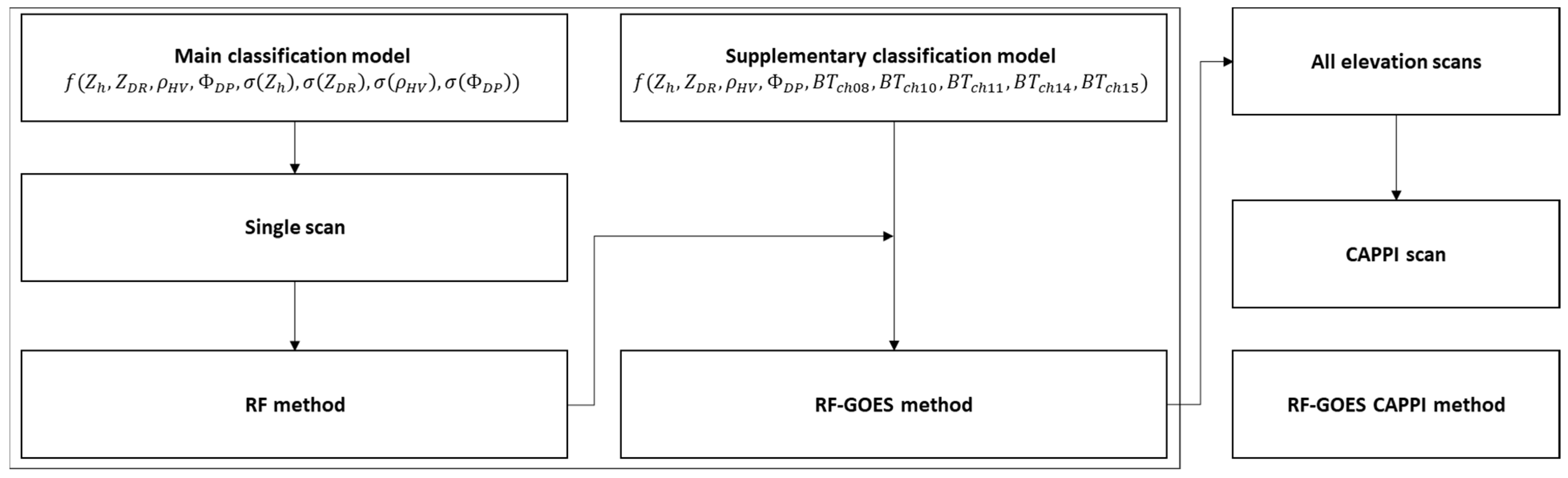
Figure 1. Framework of the study.
Remotesensing 18 00827 g001
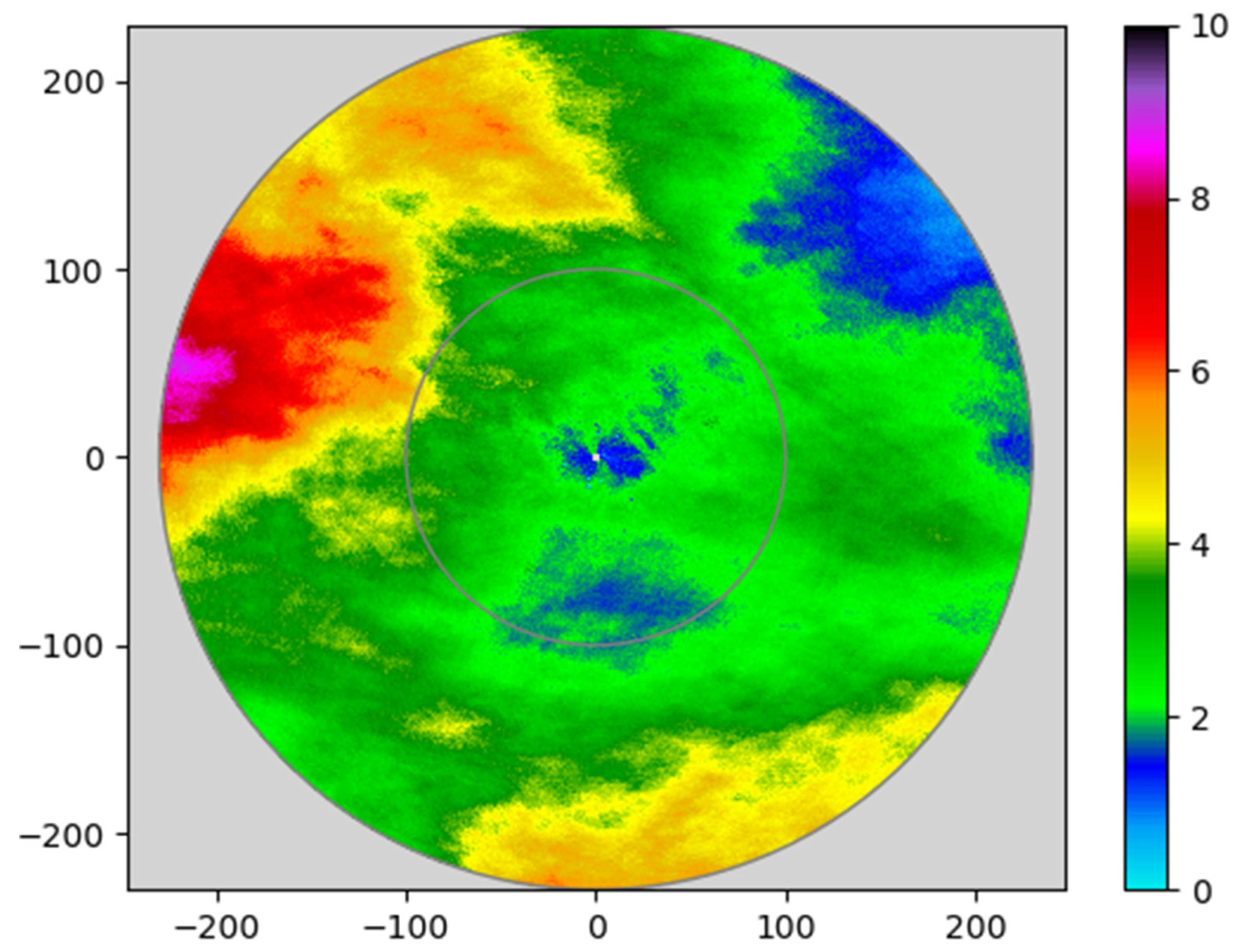
Figure 2. Study area and radar sites. Locations of the seven NEXRAD radars covering the state of Iowa are shown as black dots, with their effective ranges (230 km) indicated by gray circles. Wind turbine locations are marked with red dots.
Remotesensing 18 00827 g002
Figure 3. Maps of radar variables measured by the KDMX radar at 07:59:41 UTC on 11 June 2015. Precipitation areas are labeled as P (blue) and non-precipitation areas as NP (red). Figures generated using NOAA’s Weather and Climate Toolkit (https://www.ncdc.noaa.gov/wct/ (accessed on 12 May 2025)).
Remotesensing 18 00827 g003
Figure 4. Distributions of radar variables for P (blue) and NP (orange) echoes at sample pixels. All samples were collected from April to October 2017. The red line shows Gini Gain values (right y-axis) across varying threshold values.
Remotesensing 18 00827 g004
Figure 5. Same as Figure 4, but showing local variability of radar variables, expressed as the standard deviation within a 13 × 13 pixel window centered at each sample pixel for P (blue) and NP (orange) echoes.
Remotesensing 18 00827 g005
Figure 6. Effect of local variability estimates at multiple scales defined by various window sizes on classification accuracy and Heidke Skill Score (HSS). Bar charts show accuracy for out-of-bag (OOB, blue) and test (orange) samples. The gray line indicates HSS values for the corresponding window sizes on the test samples. The number of samples in the OOB and test datasets are 14,092,843 and 14,072,842, respectively.
Remotesensing 18 00827 g006
Figure 7. Reflectivity maps (dBZ) before (ac) and after NP echo removal by the IFC algorithm (df) and the main RF models (gi), based on KDMX radar observations at 02:48:02 UTC on 1 July 2017. The first and last columns show zoomed-in views of reflectivity for the red box areas in panels (b,e,h).
Remotesensing 18 00827 g007
Figure 8. Example of overshooting. Reflectivity maps (dBZ) before (a,b) and after NP echo removal by the IFC algorithm (c) and the main RF model (d). Raw reflectivity data are shown for the first (0.48°) and second (1.45°) elevation angle scans. Data was recorded by the KDMX radar at 07:21:07 UTC on 1 July 2017.
Remotesensing 18 00827 g008
Figure 9. Probability of rainfall detection (PORD, %) for August 2017 estimated using (a) raw reflectivity data, and reflectivity filtered by (b) IFC and (c) RF models, conditional on reflectivity > 20 dBZ. Inner and outer circles indicate 100 km and 230 km ranges from the radar, respectively. The red circle in panel (c) highlights residual wind turbine effects (speckles with high PORD values) and areas of measurement noise near the radar.
Remotesensing 18 00827 g009
Figure 10. Same as Figure 4, but for brightness temperatures from five GOES-16 infrared channels. Brightness temperature (BT) subscripts denote the channel numbers. Channels correspond to: B T c h 08 —upper-level tropospheric water vapor, B T c h 10 —lower-level tropospheric water vapor, B T c h 11 —cloud-top phase, B T c h 14 —infrared longwave, and B T c h 15 —dirty infrared longwave bands.
Remotesensing 18 00827 g010
Figure 11. Same as Figure 9, but using reflectivity filtered by the combined RF model (RF-GOES). The main RF model first removes NP echoes, followed by application of the supplementary model to the outputs of the main model.
Remotesensing 18 00827 g011
Figure 12. Reflectivity maps at 0.48° (a) and 1.32° (b) elevation angles after NP echo removal by the main RF model. Vertical profiles of reflectivity ( Z ) (c) and cross-correlation coefficient ( ρ H V ) (d) are shown at 70° azimuth. Red horizontal lines mark the 1.5 km altitude. Observations were recorded by KDMX radar at 05:04:29 UTC on 2 August 2017.
Remotesensing 18 00827 g012
Figure 13. Comparison between base scan ((a), RF-GOES) and CAPPI scan ((b), RF-GOES CAPPI at 1.5 km altitude) reflectivity (Z in dB) after NP echo removal, based on KDMX radar data at 06:31:57 UTC on 1 July 2018. The red circle indicates the area where higher-elevation reflectivity data were used to fill gaps misclassified at the lowest elevation.
Remotesensing 18 00827 g013
Figure 14. As in Figure 9, but showing the PORD map (%) derived from reflectivity filtered by the RF-GOES model and composited using the CAPPI scan strategy at 1.5 km altitude.
Remotesensing 18 00827 g014
Figure 15. (a) Azimuthally averaged PORD (%) as a function of range, and (b) radially averaged PORD (%) as a function of azimuth. The profiles were derived from the PORD maps for August 2017 generated by the RF, RF-GOES, and RF-GOES CAPPI models (Figure 9, Figure 11 and Figure 14, respectively).
Remotesensing 18 00827 g015
Figure 16. PORD maps over Iowa from April to October 2018, derived from various radar rainfall products. Red circles mark potential NP echoes caused by wind turbine effects that were not filtered by MRMS and STAGE IV algorithms.
Remotesensing 18 00827 g016
Figure 17. Hourly PORD comparison with rain gauges from April to October 2018 (RMSE: Root Mean Square Error, MAE: Mean Absolute Error, Corr: Pearson correlation coefficient).
Remotesensing 18 00827 g017
Table 1. Contingency table used to compute POD, FAR, and HSS.
Reference
PredictionClassNPP
NPa = hitb = False alarm
Pc = missd = correct negative
Table 2. Descriptive statistics of radar variables and their local variability estimates. Local variability was calculated using a 13 × 13 pixel window. All statistics were derived from the entire dataset (56,291,370 samples).
VariablesPNP
MeanMedianSTDIQRMeanMedianSTDIQR
Z h 25.0425.509.9314.008.687.506.168.50
Z D R 0.510.441.021.002.532.633.594.81
ρ H V 0.981.000.050.020.740.780.220.30
Φ D P 69.5566.2915.5811.28101.7492.0353.9052.54
σ ( Z h ) 4.703.802.712.624.423.842.252.75
σ ( Z D R ) 1.340.801.390.823.643.291.602.16
σ ( ρ H V ) 0.090.030.140.080.230.210.090.12
σ ( Φ D P ) 10.115.9610.257.9246.8146.2320.3029.06
Table 3. Performance metrics for NP echo detection by range. Zones 1–3 correspond to distance ranges of 0–75 km, 75–150 km, and 150–230 km, respectively, from which test samples were drawn.
StatisticsIFCRF
Zone 1Zone 2Zone 3Zone 1Zone 2Zone 3
POD0.99820.99971.00001.00001.00000.9995
FAR0.01690.13390.77050.00010.00030.0041
HSS0.85450.77290.25160.99920.99950.9974
Table 4. Spatial derivatives of azimuthally and radially averaged PORD. Zone definitions follow those in Table 3, except for Zone 1, which spans 5–75 km to exclude the effects of the cone of silence. Radially averaged PORD was computed over the 75–125 km range to minimize contamination from ground clutter near the radar.
ModelRadial Derivatives of Azimuthally Averaged PORD (%)Azimuthal Derivatives of Radially Averaged PORD
Zone 1Zone 2Zone 3
MeanSTDSTD
Reduction
MeanSTDSTD
Reduction
MeanSTDSTD
Reduction
MeanSTDSTD
Reduction
Raw−0.030.14-0.000.05-0.000.01-0.000.15-
RF0.000.0193.64%0.000.0089.38%0.000.0033.05%0.000.0284.65%
RF-GOES0.000.0193.93%0.000.0090.17%0.000.0032.01%0.000.0285.49%
RF-GOES CAPPI0.000.0096.59%0.000.0092.81%0.000.0057.28%0.000.0285.51%
Disclaimer/Publisher’s Note: The statements, opinions and data contained in all publications are solely those of the individual author(s) and contributor(s) and not of MDPI and/or the editor(s). MDPI and/or the editor(s) disclaim responsibility for any injury to people or property resulting from any ideas, methods, instructions or products referred to in the content.