Article

Impacts of Climate Change, Human Activities, and Their Interactions on China’s Gross Primary Productivity

1
Key Laboratory of Ecosystem Carbon Source and Sink, China Meteorological Administration, Wuxi University, Wuxi 214105, China
2
CAS Key Laboratory of Forest Ecology and Silviculture, Institute of Applied Ecology, Chinese Academy of Sciences, Shenyang 110016, China
3
University of Chinese Academy of Sciences, Beijing 101408, China
4
Zhejiang Institute of Meteorological Science, Hangzhou 310008, China
5
College of Meteorology and Oceanography, National University of Defense Technology, Changsha 410073, China
*
Author to whom correspondence should be addressed.
These authors contributed equally to this work.
Remote Sens. 2026, 18(2), 275; https://doi.org/10.3390/rs18020275
Submission received: 6 November 2025 / Revised: 1 January 2026 / Accepted: 9 January 2026 / Published: 14 January 2026

Highlights

What are the main findings?
  • Gross primary productivity (GPP) exhibited a significant upward trend nationwide, especially in deciduous broadleaf forests, croplands, grasslands and savannas.
  • The SHAP−based analysis revealed Leaf area index (LAI) as the strongest positive driver, while nonlinear interactions with radiation, temperature, and water availability jointly regulate GPP.
What are the implications of the main findings?
  • GPP variations in China are controlled by ecosystem-specific interactions among vegetation, climate, topography, and human activities, indicating that a uniform management or restoration strategy is ineffective across ecosystems.
  • The identified dominant drivers suggest targeted ecosystem management strategies: forest management should consider and maintain the interactions between climate and vegetation structure; grassland restoration should prioritize topographic constraints; and cropland productivity should depend strongly on management practices.
  • Incorporating these nonlinear and ecosystem-dependent interactions into carbon cycle models can improve projections of ecosystem productivity under climate change, thereby supporting climate adaptation planning and ecosystem protection strategies.

Abstract

Gross Primary Productivity (GPP) plays a vital role in the terrestrial carbon cycle and ecosystem functioning. Understanding its spatio-temporal dynamics and driving mechanisms is critical for predicting ecosystem responses to climate change. China’s GPP has experienced complex responses due to heterogeneous climate, environment, and human activities, yet their impacts and interactions across ecosystems remain unquantified. This study used the Mann–Kendall test and SHapley Additive exPlanations to quantify the contributions and interactions of climate, vegetation, topography, and human factors using GPP data (2001–2020). Nationally, GPP showed a significant upward trend, particularly in deciduous broadleaf forests, croplands, grasslands, and savannas. Leaf area index (LAI) is identified as the primary contributor to GPP variations, while climate factors exhibit nonlinear interactive effects on the modeled GPP. Ecosystem-specific sensitivities were evident: forest GPP is predominantly associated with climate–vegetation coupling. Additionally, in coniferous forests, the interaction between anthropogenic factors and topography shows a notable association with productivity patterns. Grassland GPP is primarily linked to topography, while cropland GPP is mainly related to management practices and environmental conditions. In contrast, the GPP of savannas and shrublands is less influenced by factor interactions. These findings high-light the necessity of ecosystem-specific management and restoration strategies and provide a basis for improving carbon cycle modeling and climate change adaptation planning.

1. Introduction

Gross Primary Productivity (GPP), defined as the amount of organic carbon fixed by living organisms (mainly green plants) through photosynthesis, is a key component of the terrestrial carbon cycle, as it determines the initial input of matter and energy into terrestrial ecosystems [1,2]. Together with ecosystem respiration, GPP governs the CO2 flux between land and atmosphere, thus playing a crucial role in regulating atmospheric CO2 levels and mitigating climate change [3,4]. Moreover, GPP underpins the production of food, fiber, and wood, making it vital to human welfare. Therefore, understanding the spatiotemporal variations of GPP and its driving mechanism is essential for predicting ecosystem responses to environmental changes and informing sustainable land management practices [5,6].
In recent years, many studies have reported widespread GPP increases across the Northern Hemisphere, largely attributable to extended growing seasons under warmer and wetter conditions [7,8,9]. However, some regions exhibit declining trends, likely due to warming-induced drought stress that offsets spring carbon gains [8,10]. In China, pronounced climate changes have strongly influenced vegetation growth and carbon sequestration [11,12]. Overall increases in GPP have been observed, particularly in the Loess Plateau and southern China [13,14]. Regionally, from 1982 to 2017, the Three−North Region of China exhibited an increasing GPP trend, attributed to climate change, rising atmospheric CO2 concentrations, and human activities [15], represented by land-use intensity and management-related factors (e.g., cropland management, irrigation, and afforestation). Similarly, the Yangtze River Basin experienced a 7.9% increase in GPP between 2000 and 2009, particularly in its southwestern sections [16]. On the Yungui Plateau, a significant upward trend occurred in the northeast, contrasted with a slight decline in the south [17]. These findings collectively highlight strong spatial heterogeneity in GPP responses, arising from diverse climate regimes, land-cover patterns, topographic conditions, and human activities across China [18]. However, most existing studies focus on specific regions or vegetation types, and a systematic, nationwide synthesis that explicitly compares GPP dynamics across major eco-systems remains limited.
Furthermore, GPP is influenced by multiple interacting factors. Climate drivers, such as temperature, precipitation, and radiation, directly affect plant physiological processes [19,20]. These factors exhibit spatiotemporal variability and elicit vegetation-type-dependent responses [21,22]. For instance, Yue et al. [23] found that CO2 fertilization dominates GPP increases in forests, whereas meteorological factors prevail in grasslands and shrublands. Warming enhances summer GPP at high latitudes but reduces carbon uptake in tropical regions due to drought. Moreover, extreme events like droughts and heatwaves have significantly reduced ecosystem carbon storage, exemplified by an approximate 30% decline in European plant productivity [24]. Concurrently, globalization intricately interacts with urbanization, land-use change, and policy interventions, profoundly shaping socioeconomic and ecological outcomes worldwide. These human activities collectively modify ecosystem structure and function, further modulating carbon dynamics [25]. For example, Naeem et al. [26] reported an increase in net primary productivity in China following the expansion of the human footprint after 2000. Liu et al. [27] revealed that, under urbanization, GPP in urban core areas significantly increased, while it significantly decreased in urban expansion areas, primarily due to substantial vegetation loss caused by land use conversion. Similarly, Xue et al. [28] demonstrated that between 2000 and 2018, grassland GPP dynamics in seven Chinese provinces/autonomous regions were primarily influenced by human activities, including socioeconomic factors, livestock farming, and national policies. Additionally, Luo et al. [29] found that the construction and operation of the Qinghai–Tibet Railway, which began in 2001 and became fully operational in 2006, promoted local economic growth through increased human activity and tourism, yet also contributed to alpine vegetation degradation, particularly in the southern part of the Qinghai–Tibet Engineering Corridor.
Despite these advances, two critical knowledge gaps remain. First, most attribution studies focus on the relative importance of individual drivers, while the extent to which nonlinear interactions among climate, vegetation, topography, and human activities jointly regulate GPP remains poorly quantified, especially across different ecosystem types. For instance, studies focusing on grassland ecosystems in China, such as Xue et al. [28], have demonstrated that human activities and socioeconomic factors strongly influence GPP dynamics; however, these analyses largely treat drivers as additive effects and do not explicitly quantify interactions among multiple environmental and anthropogenic factors. Consequently, it remains unclear whether such interactions are secondary influences or fundamental components of ecosystem productivity regulation.
Second, although human activities are widely recognized as important drivers, their effects are often represented using aggregated proxies, which obscure how specific anthropogenic pressures interact with environmental conditions to shape GPP. Liu et al. [30] employed the residual trend (RESTREND) approach to separate the respective contributions of climate change and human activities to variations in Normalized Difference Vegetation Index (NDVI), Vegetation Optical Depth (VOD), and GPP, showing that human activities contributed more strongly than climate factors to GPP increases in many regions. While informative, this approach quantifies only the overall contribution of human activities and does not explicitly resolve how management practices, land-use intensity, or landscape structure modify climate–vegetation relationships. Conventional multiple linear regression and correlation-based approaches are ill suited to disentangle these complex, nonlinear, and ecosystem-dependent interactions, leaving the quantitative contribution of anthropogenic–environmental interactions largely unresolved.
To address these gaps, we employ a machine-learning-based interpretability framework that integrates Extreme Gradient Boosting (XGBoost) with SHapley Additive exPlanations (SHAP). For each vegetation type, GPP is modeled as a nonlinear function of climate, vegetation, topography, and human activity variables. XGBoost is not used merely as a predictive algorithm, but as a flexible nonlinear function approximator that captures complex interactions among these predictors. SHAP values are then computed to decompose the contributions of individual factors and their two-way interactions to GPP variation. Factor-level contributions are calculated as the absolute SHAP value of each predictor divided by the sum of all predictors’ absolute SHAP values, while category-level contributions (climate, vegetation, topography, human activity) are the sum of their constituent factors’ SHAP values. Two-way interactions are quantified using SHAP interaction values, enabling the assessment of synergistic or antagonistic effects among factors. This approach allows identification of dominant drivers and key interactions, providing an interaction-centered understanding of GPP regulation across ecosystems. Unlike conventional methods, this framework moves beyond evaluating only additive effects, enabling explicit characterization of ecosystem-specific interaction regimes. While previous studies have applied SHAP to identify climatic controls on GPP variability [31], few have simultaneously quantified the interactive effects of climate, vegetation, topography, and human activities at the national scale. Accordingly, this study addresses the following questions: (1) How do climate, vegetation, topography, and human activities individually and interactively influence GPP across China? (2) Do interaction effects differ systematically among major ecosystem types? By combining Mann–Kendall trend analysis with SHAP−based attribution, this study provides a mechanistic, interaction-centered interpretation of GPP regulation, offering new insights into terrestrial carbon-cycle dynamics and supporting ecosystem-specific management under climate change and carbon neutrality goals.
The remainder of this paper is structured as follows: Section 2 describes the study domain, datasets, and methodologies. Section 3 presents the analysis of GPP trends and their attribution. Section 4 focuses on how the interactions among factors influence GPP in different ecosystems. Section 5 summarizes the key conclusions. All abbreviations used in this study are summarized in Table S1.

2. Materials and Methods

2.1. Study Domain

This study focuses on the terrestrial ecosystems of mainland China (18.5° N–53.75° N, 73.25° E–135.25° E), with a total area of approximately 9.6 million km2. China exhibits highly diverse topography, characterized by a three-step terrain descending from the high plateaus in the west to the plains in the east, as illustrated in Figure 1a. The country spans multiple climate zones, ranging from cold temperate to tropical regions (Figure 1b). China’s terrestrial ecosystems are remarkably diverse, consisting primarily of forests (Evergreen Needleleaf Forest (ENF), Evergreen Broadleaf Forest (EBF), Deciduous Needleleaf Forest (DNF), Deciduous Broadleaf Forest (DBF), Mixed Forest (MF)), grasslands, croplands, savannas, and shrublands (Figure 1c). Forests are mainly distributed in the northeast, southwest, and southeastern coastal regions and represent the major carbon sinks in China. Grasslands are widely distributed across the Qinghai–Tibet Plateau and the Inner Mongolian Plateau, playing crucial roles in regional carbon cycling and water regulation. Croplands are mainly concentrated in the eastern plains, where human activities are particularly intensive. Savannas and shrublands are primarily found in southern and southwestern China, especially in transitional zones between forests and grasslands. Spanning arid to humid and cold-temperate to tropical zones, the study domain offers an ideal natural laboratory for tracing GPP dynamics across climates and ecosystems [32].

2.2. Datasets

2.2.1. PML−V2 (China) GPP Dataset

The Penman−Monteith–Leuning Version 2 (PML−V2) (China) terrestrial GPP dataset [34] was obtained from the National Tibetan Plateau Data Center (https://data.tpdc.ac.cn/en/data/40f57c67-33a6-402d-bd37-6ede91919f23 (accessed on 5 January 2026)). This dataset provides daily GPP estimates across China from 26 February 2000 to 31 December 2020, with a spatial resolution of 500 m. It was generated using the PML−V2 water–carbon coupled model, which estimates GPP by integrating atmospheric and vegetation observations. Owing to its high accuracy [34,35], this dataset was used in this study for trend analysis and SHAP−based factor attribution, after spatial harmonization with other predictors.

2.2.2. MODIS Land Cover and MODIS−Derived LSWI

This study used the Moderate Resolution Imaging Spectroradiometer (MODIS) Land Cover (MCD12Q1) product (https://ladsweb.modaps.eosdis.nasa.gov/missions-and-measurements/products/MCD12Q1 (accessed on 5 January 2026)) to classify ecosystem types across the study domain. This product provides yearly 500 m global land-cover maps from 2001 onward. We selected the classification scheme following the International Geosphere−Biosphere Programme system [36].
This study used the Land Surface Water Index (LSWI) derived from the MODIS MOD09A1 8−day, 500 m surface reflectance product (https://ladsweb.modaps.eosdis.nasa.gov/missions-and-measurements/products/MOD09A1 (accessed on 5 January 2026)) to characterize vegetation and soil water status. The calculation formula is as follows [37]:
L S W I = N I R S W I R N I R + S W I R
where NIR and SWIR represent the near-infrared and shortwave infrared bands, respectively. Ecologically, LSWI reflects vegetation water status and soil moisture availability, both of which directly regulate photosynthetic activity by influencing stomatal conductance, leaf turgor, and biochemical processes. Consequently, LSWI serves as an effective proxy for water-related constraints on GPP, particularly in water-limited or seasonally dry ecosystems.

2.2.3. CMFD Meteorological Dataset

The China Meteorological Forcing Dataset (CMFD) meteorological variables [38], obtained from the National Tibetan Plateau Data Center (https://www.tpdc.ac.cn/zh-hans/data/e60dfd96-5fd8-493f-beae-e8e5d24dece4 (accessed on 5 January 2026)), served as the climatic predictors in the attribution analysis. This dataset covers 1951–2024 at 3-hourly, 0.1° resolution. We used precipitation (PRECIP, mm), surface pressure (PSFC, Pa), downward shortwave radiation (SWDOWN, W m−2), air temperature (T2D, K), and specific humidity (Q, kg kg−1) from the dataset. Based on these variables, relative humidity (RH, %) and vapor pressure deficit (VPD, Pa) were further calculated using the following formulas [39,40]:
t c = T 2 D 273.15
e s = 610.78 × e x p ( ( 17.27 × t c ) / ( t c + 237.3 ) )
e a = ( Q × P S F C ) / ( 0.622 + 0.378 × Q )
R H = ( e a e s ) × 100 %
V P D = e s e a
where t c is the temperature in degrees Celsius, e s is the saturation vapor pressure, and e a is the actual vapor pressure.

2.2.4. GLASS LAI Dataset

The Global Land Surface Satellite Leaf Area Index V60 (GLASS LAI V60) product, obtained from the National Earth System Science Data Center (https://glass-product.bnu.edu.cn/introduction1/LAI.html (accessed on 5 January 2026)), was used as the vegetation factor in the attribution analysis. This dataset provides 8−day composite LAI estimates at a spatial resolution of 1 km from 2000 to the present. It was generated using a general regression neural network algorithm that incorporates preprocessed MODIS surface reflectance data over continuous annual cycles [41], enabling more robust temporal profile estimation compared to single-date retrieval methods. The accuracy and long-term consistency of this dataset have been extensively validated [42,43].

2.2.5. SRTM DEM Dataset

Elevation, slope, and aspect derived from the Shuttle Radar Topography Mission (SRTM) Digital Elevation Model (DEM) (https://doi.org/10.5067/MEASURES/SRTM/SRTMGL1.003 (accessed on 5 January 2026)) at a spatial resolution of 30 m were used as topographic factors in the attribution analysis. The slope (in degrees) and aspect (in degrees, with north as 0°) were calculated using standard spatial analysis algorithms based on the elevation data [44]. These topographic variables were subsequently aggregated to a coarser grid for consistency with other predictors, as described in Section 2.2.7.

2.2.6. Human Activity Factors

Human activities were represented using proxy indicators that characterize the intensity and spatial configuration of anthropogenic pressure at the grid scale. In this study, two types of indicators were used to characterize human activity and landscape patterns. The Human Influence Index (HII), obtained from the Wildlife Conservation Society (WCS) (https://www.wcshumanfootprint.org/data-access (accessed on 5 January 2026)), was used to quantify the intensity of human activities. The dataset provides annual data with a spatial resolution of 1 km, representing the cumulative impact of multiple anthropogenic pressures such as population density, land use, infrastructure, and human accessibility [45]. From an ecological perspective, higher HII values are generally associated with increased habitat modification, landscape fragmentation, and disturbance intensity, which can alter vegetation structure, species composition, and resource availability. These changes influence GPP through multiple pathways, including reductions in vegetation cover, disruption of ecological connectivity, and long-term disturbance legacies. Therefore, HII provides a macro-scale proxy for assessing the cumulative intensity of human influence on ecosystem productivity, rather than the effects of specific management practices.
In addition, three landscape pattern indices—patch density (PD), landscape shape index (LSI), and aggregation index (AI)—were employed to describe the spatial configuration of ecosystems. These indices were calculated as follows [46]:
P D i = n i / a i
L S I i = 0.25 k = 1 m e i , k a i
A I i = [ 1 + j = 1 n i P i , j ln ( P i , j ) / 2 ln ( n i ) ] × 100
where n i , a i , and e i are the number of patches, the total area (km2), and the total boundary length (km) of a specific vegetation type in region i , respectively. e i , k is the perimeter (km) of patch k of the vegetation type in county i , m is the total number of patches (i.e., n i ). P i , j denotes the perimeter (km) of patch j of the same vegetation type in county i . A higher P D i and L S I i , together with a lower A I i , indicate a greater degree of landscape fragmentation for that vegetation type within county i .

2.2.7. Spatial Harmonization of Datasets

All datasets used in this study were harmonized to a common spatial resolution of 0.1° (approximately 10 km at the equator) to ensure consistency within the modeling framework. Variables with finer native resolutions were spatially aggregated to the 0.1° grid using appropriate statistical summaries. Specifically, slope was aggregated using mean values within each grid cell, while aspect was first transformed into sine and cosine components to account for its circular nature and then averaged to represent dominant terrain orientation.
After spatial harmonization, spatiotemporal samples were constructed from the processed 0.1° gridded data. Each sample represents a unique space–time unit defined by a 0.1° grid cell and a specific year, containing annual mean values of GPP and all predictor variables.
The derivation process was as follows: First, annual masks for each vegetation type of interest (e.g., deciduous broadleaf forest, grassland) were created based on the MODIS MCD12Q1 land cover classification. For each year from 2001 to 2020, all grid cells identified as a given vegetation type were extracted. The corresponding values for climate, vegetation indices, topography, human activity factors, and GPP were assigned to each cell, forming the annual sample pool for that vegetation type. Annual samples were then aggregated across the entire study period (2001–2020) to create the complete sample set for each vegetation type.
Two types of model datasets were compiled: (1) an Overall Dataset combining samples from all vegetation types across China, and (2) Vegetation-Specific Datasets for each major ecosystem type. Each dataset was randomly partitioned into a training set (70% of samples) for model calibration and hyperparameter optimization, and an independent test set (30%) for model validation.

2.3. Mann–Kendall Trend Analysis

In this study, the Mann–Kendall (MK) trend test [47,48,49,50] was employed to analyze the multi-year and seasonal trends of GPP across China. The MK test was a widely used non-parametric method for detecting trends in time-series data and is particularly suitable for ecological datasets, which often exhibit non-normal distributions and may contain outliers or missing values. For a given GPP time series ( X 1 , X 2 , , X n ), Kendall’s S statistic is calculated as:
S = i = 1 n 1 j = i + 1 n s g n ( X j X i )
s g n ( X j X i ) = { 1 ( X j X i ) > 0 0 ( X j X i ) = 0 1 ( X j X i ) < 0
The significance of the trend is assessed using the standardized test statistic Z :
Z = { S 1 V a r ( S ) S > 0 0 S = 0 S + 1 V a r ( S ) S < 0
V a r ( S ) = 1 18 [ n ( n 1 ) ( 2 n + 5 ) ]
A positive Z indicates an increasing trend, while a negative Z indicates a decreasing trend. A significance level of 95% was adopted, meaning a trend is considered significant when | Z | 1.96 .
The magnitude of the trend was quantified using Sen’s slope estimator β :
β = m e d i a n ( X j X i j i ) 1 < i < j < n
This approach allowed us to identify both the direction and the rate of change in GPP over the study period across different regions in China.

2.4. XGBoost Algorithm and SHapley Additive exPlanations

In this study, we employed the XGBoost algorithm [51] in combination with SHapley Additive exPlanations (SHAP) [52] to model and interpret the factors influencing GPP across China. The model incorporated four groups of predictors: climatic factors (i.e., PRECIP, PSFC, RH, SWDOWN, T2D, VPD), vegetation factors (i.e., LAI, LSWI), topographic factors (i.e., elevation, slope, aspect), and human activity factors (i.e., HII, PD, LSI, AI).
XGBoost is a gradient boosting framework that constructs an ensemble of decision trees. It offers high predictive accuracy and is robust to multicollinearity and non-linear relationships among factors [53]. To quantify the contribution of each factor, we applied the SHAP method, which provides a unified measure of feature importance based on cooperative game theory [54,55]. In cooperative game theory, each feature is treated as a “player” in a coalition of all features, and the Shapley value quantifies the average contribution of that feature to the model prediction across all possible combinations. This approach ensures that the influence of each feature is fairly and systematically allocated. SHAP values reflect both the magnitude and direction of each variable’s influence on GPP, enabling a detailed understanding of the underlying climatic, environmental, and ecological drivers.
The SHAP method is used to calculate SHAP values of each input variable as follows [54]:
f ( x ) = φ 0 + i = 1 N φ i
where f ( x ) represents the simulated GPP value. φ 0 is the mean value of predicted GPP, and φ i is the SHAP value for factor i .
For each feature, SHAP values can be divided into main and interactive effects based on the Shapley interaction index as follows [56,57]:
φ i = Φ i , i + i j Φ i , j
where φ i represents SHAP values (total effects) for factor i , including Φ i , i (main effects) and Φ i , j (interactive effects with other factors).
To facilitate comparisons across different vegetation types with varying baseline GPP values, we calculated the SHAP percentage (%), defined as the ratio of each original SHAP value to the mean predicted GPP [19]:
S H A P   p e r c e n t a g e i   ( % ) =   φ i φ 0   × 100
Additionally, to isolate the contribution of individual factors to GPP variability, we computed the SHAP contribution (%), defined as the ratio of the absolute SHAP value of a factor to the sum of absolute SHAP values of all factors:
S H A P   c o n t r i b u t i o n i   ( % ) =   | φ i | i | φ i |   × 100
S H A P   i n t e r a c t i o n   c o n t r i b u t i o n i , j   ( % ) = | Φ i , j | i | Φ i , j | × 100
when i = j , it represents the proportion of the total effect contributed by the main effect of factor i ; when i j , it represents the proportion of the total effect contributed by the interaction between factors i and j .
This combined XGBoost–SHAP framework allows both accurate prediction of GPP and transparent evaluation of the relative importance and interactions of explanatory variables.

3. Results

3.1. Spatio−Temporal Trends of GPP over China

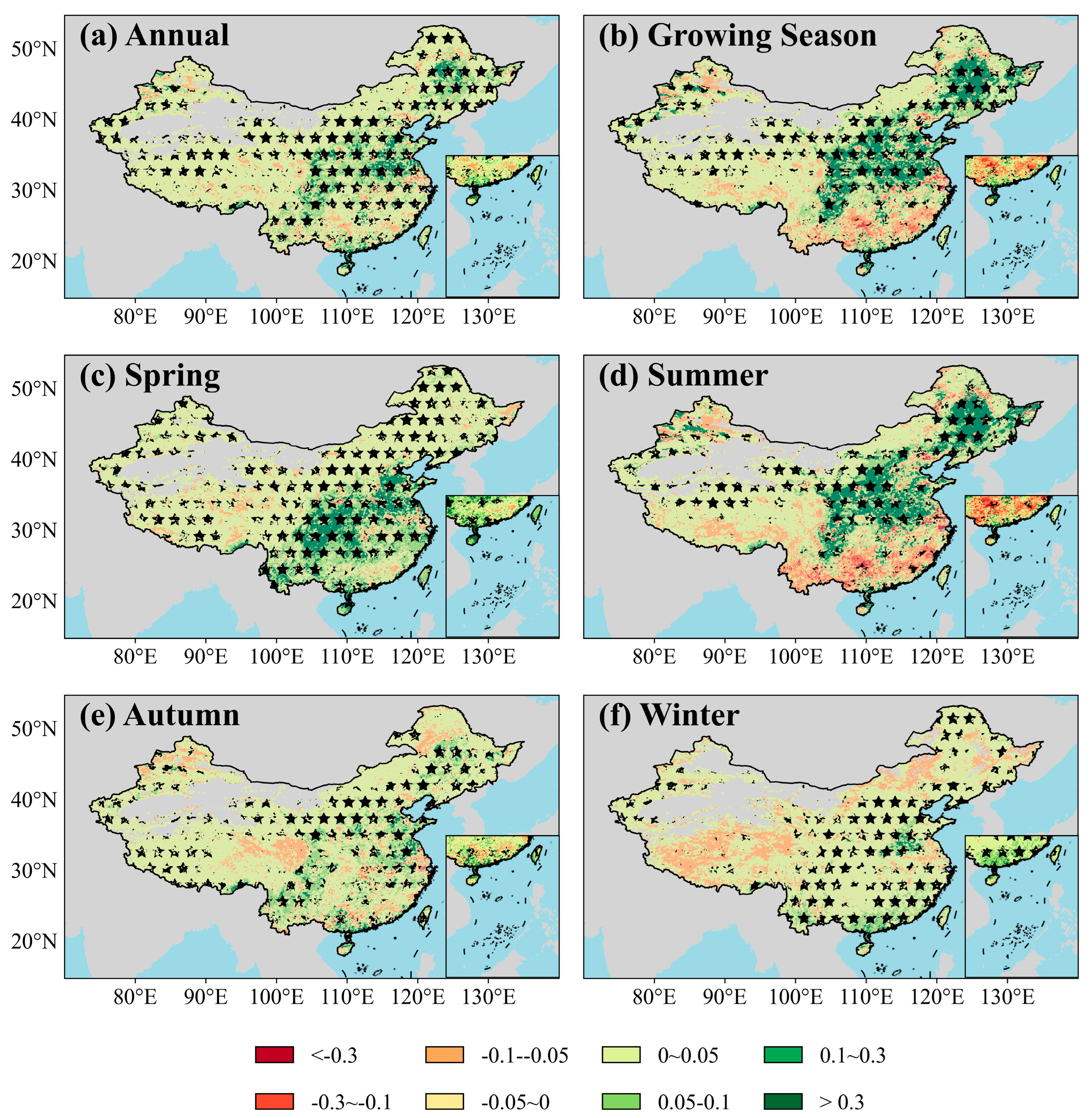
Figure 2 presents the spatio-temporal trends of annual, growing season, and seasonal mean GPP across China from 2001 to 2020. Annually, GPP rose significantly in most regions, particularly the Northeast Plain, North China Plain, and Loess Plateau (Figure 2a). During the growing season, GPP significantly increased in the Northeast Plain, the Loess Plateau, the North China Plain, the Sichuan Basin, and the northern Tibetan Plateau, but decreased in southern China, including the Jiangnan Hills and the Yunnan–Guizhou Plateau (Figure 2b). Seasonal GPP trends exhibited pronounced spatial heterogeneity. During spring (March–May), GPP increased nationwide, with the most pronounced increases in the North China Plain and Sichuan Basin (Figure 2c). During summer (June–August), GPP increased significantly in the Northeast Plain, North China Plain, and Loess Plateau, but declined in the Jiangnan Hills and Yunnan–Guizhou Plateau (Figure 2d). During autumn (September–November), GPP declined significantly across most regions of China (Figure 2e). During winter (December–February), national mean GPP increased significantly, with increases mainly occurring in south-eastern China, whereas declines were observed in the Inner Mongolia Plateau and the Tibetan Plateau (Figure 2f). However, the increases in autumn and winter were less than 0.05 g C m−2 d−1. These findings reveal the pronounced seasonal–spatial dynamics of China’s GPP.
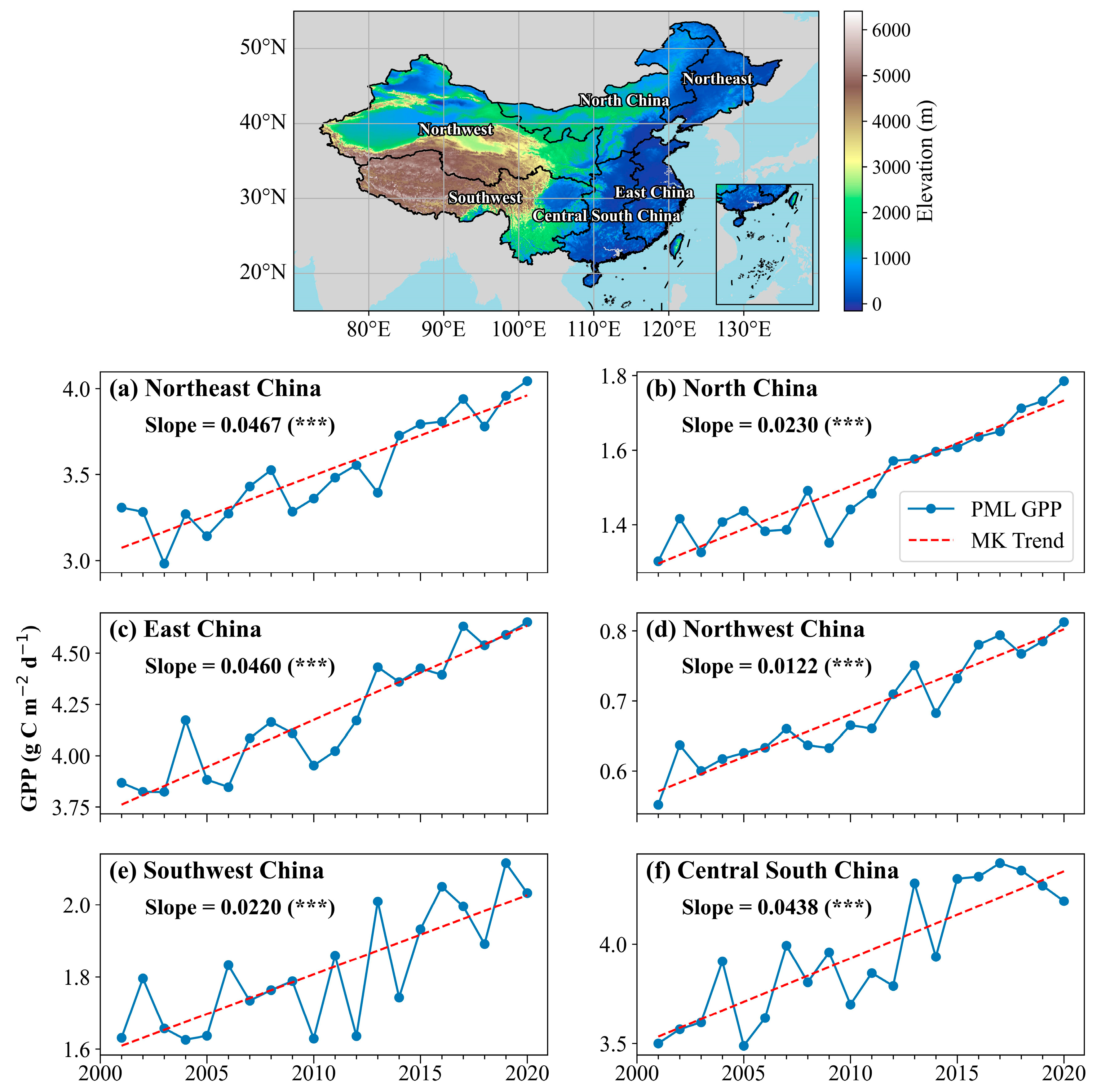
Given the spatial differences in GPP trends revealed in Figure 2, the study domain was divided into six Chinese regions, including Northeast, North, East, Northwest, Southwest, and Central South China, to investigate the trends in annual, growing season, and seasonal GPP, as shown in Figure 3. Overall, all regions exhibited significant increasing trends in GPP. Northeast (Figure 3a), East (Figure 3c), and Central South China (Figure 3f) showed the most rapid increases in GPP, with Sen’s slopes of 0.0467 g C m−2 d−1, 0.0460 g C m−2 d−1, and 0.0438 g C m−2 d−1, indicating a stronger enhancement of carbon sequestration in these regions. These results are in agreement with earlier findings [58] that highlighted similar regional enhancements in GPP across China. North (Figure 3b) and Southwest China (Figure 3e) also display significant GPP increases, but at slightly lower rates (0.0230 g C m−2 d−1 and 0.0220 g C m−2 d−1). Northwest China showed relatively smaller trends, especially the arid Northwest with a slope of 0.0122 g C m−2 d−1 (Figure 3d), suggesting that GPP growth is limited in dry regions [59,60]. Overall, GPP increases were more pronounced in eastern and northeastern China, whereas western regions had slower growth, likely due to climatic, hydrological, and vegetative conditions.

3.2. Spatio−Temporal Trends of GPP Under Different Vegetation Types

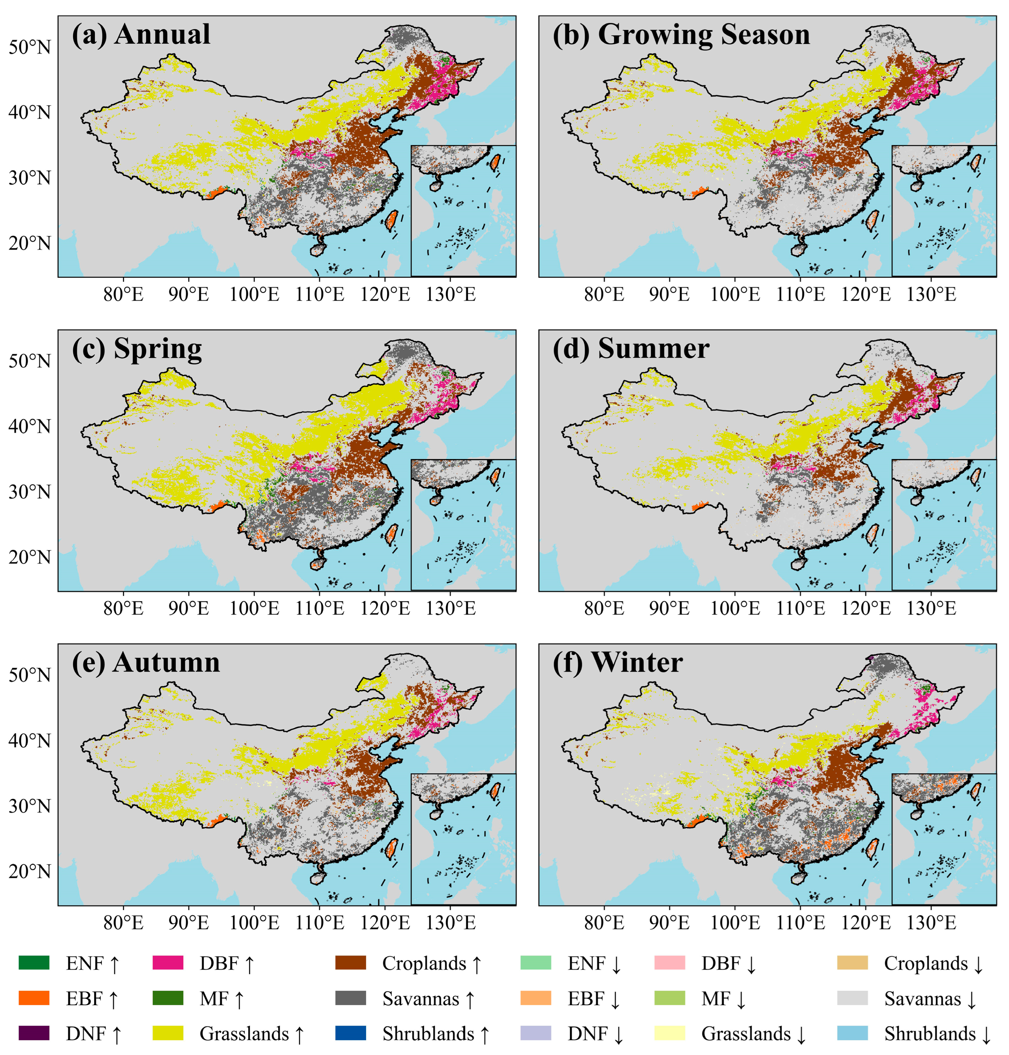
Subsequently, we examined trends in GPP for typical vegetation types in China from 2001 to 2020 (Figure 4), considering only significant pixels within areas where land cover remained unchanged. Annually, DBF, grasslands, croplands, and savannas exhibited widespread increases (Figure 4a). During the growing season, positive trends persisted in these vegetation types, although the area of savannas showing GPP increases was smaller than that observed for the annual trends (Figure 4b). In contrast, some EBF pixels exhibited significant declines during summer (Figure 4d), likely due to heat and water stress limiting photosynthesis [61]. Seasonally, GPP in DBF, grasslands, and croplands increased consistently in spring and autumn (Figure 4c,e), contributing most to the annual growth. This pattern reflects the extension of the growing season under warming conditions, which delays senescence and prolongs periods of active photosynthesis [9,62,63]. During winter, EBF exhibited increasing GPP, contrasting with its summer decline, while DBF, grasslands, croplands, and savannas also maintained positive trends (Figure 4f), likely driven by warmer temperatures and milder winters sustaining photosynthetic activity. Overall, these seasonal patterns suggest that global warming has prolonged the growing season, enhancing GPP in most vegetation types, but also inducing seasonal compensation in EBF, with summer reductions offset by winter increases [9,24].
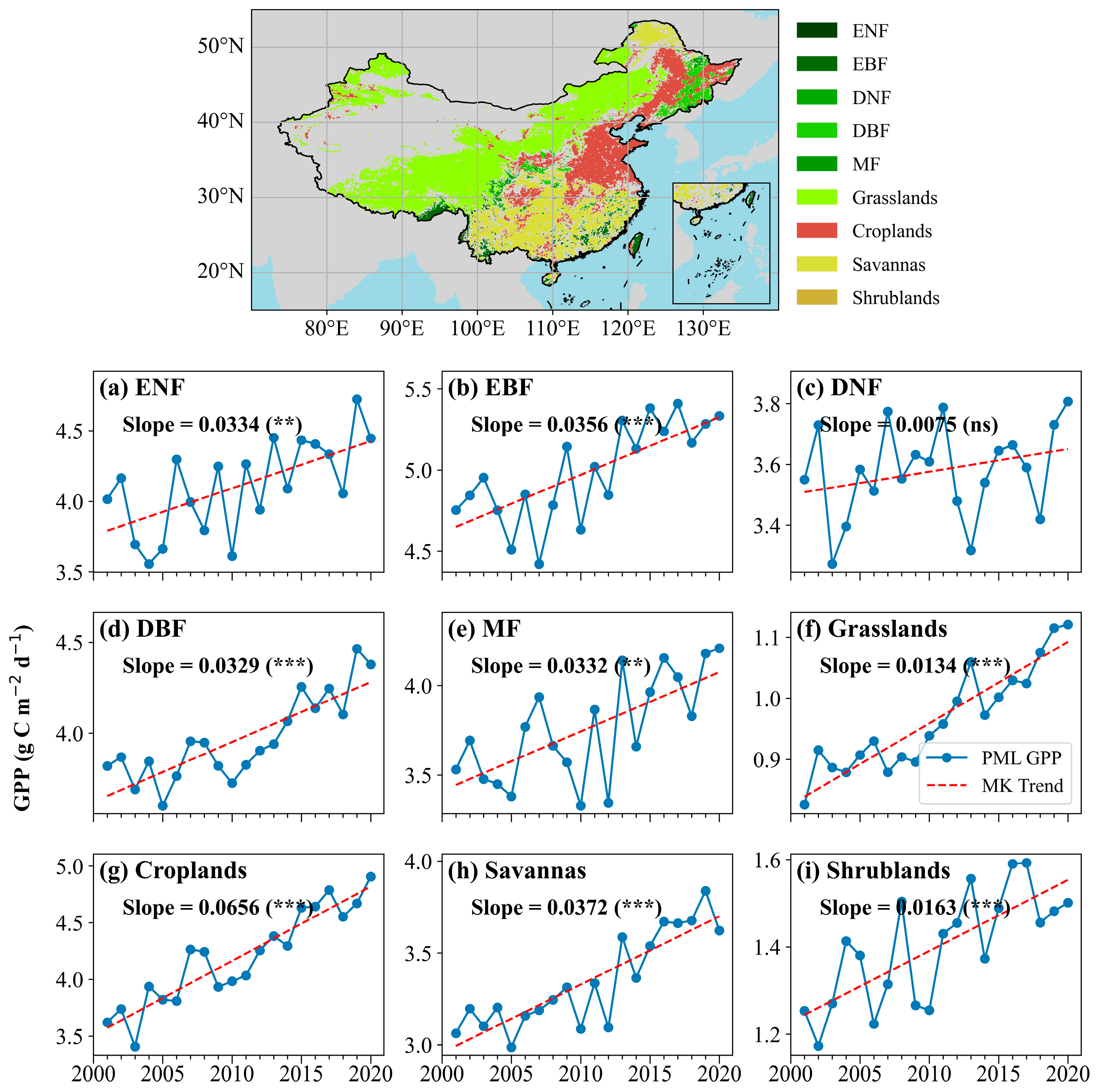
Figure 5 further quantifies the long-term GPP trends under different vegetation types from 2001 to 2020. DBF, EBF, grasslands, croplands, and savannas exhibited highly significant increasing trends, while ENF and MF also showed consistent upward trends. In contrast, DNF showed no significant change. Croplands had the largest GPP increase (0.0656 g C m−2 d−1), higher than savannas (0.0372 g C m−2 d−1), ENF (0.0334 g C m−2 d−1), MF (0.0332 g C m−2 d−1), and DBF (0.0329 g C m−2 d−1). Shrublands (0.0163 g C m−2 d−1) and grasslands (0.0134 g C m−2 d−1) had the smallest increases. These findings are consistent with a previous site-level study reporting rising GPP trends in croplands, forests, and grasslands between 2001 and 2018 [64], which indicated that grasslands and croplands experienced substantial gains, while forest growth was comparatively smaller. Overall, the results underscore the prominent contributions of croplands and forests to the national GPP increase in China.

3.3. Attribution of Spatio−Temporal Variations in GPP

This study employed the FLAML algorithm to determine the optimal hyperparameters of XGBoost (Table S3) and developed XGBoost models for different vegetation types. These models were subsequently used for factor interpretability analysis. The overall model based on all vegetation samples achieved an R2 value of 0.95 (Table S2). Vegetation-specific models had R2 values exceeding 0.75 across all vegetation types. These results validate the GPP simulation performance and the applicability of the machine learning models constructed in this study.
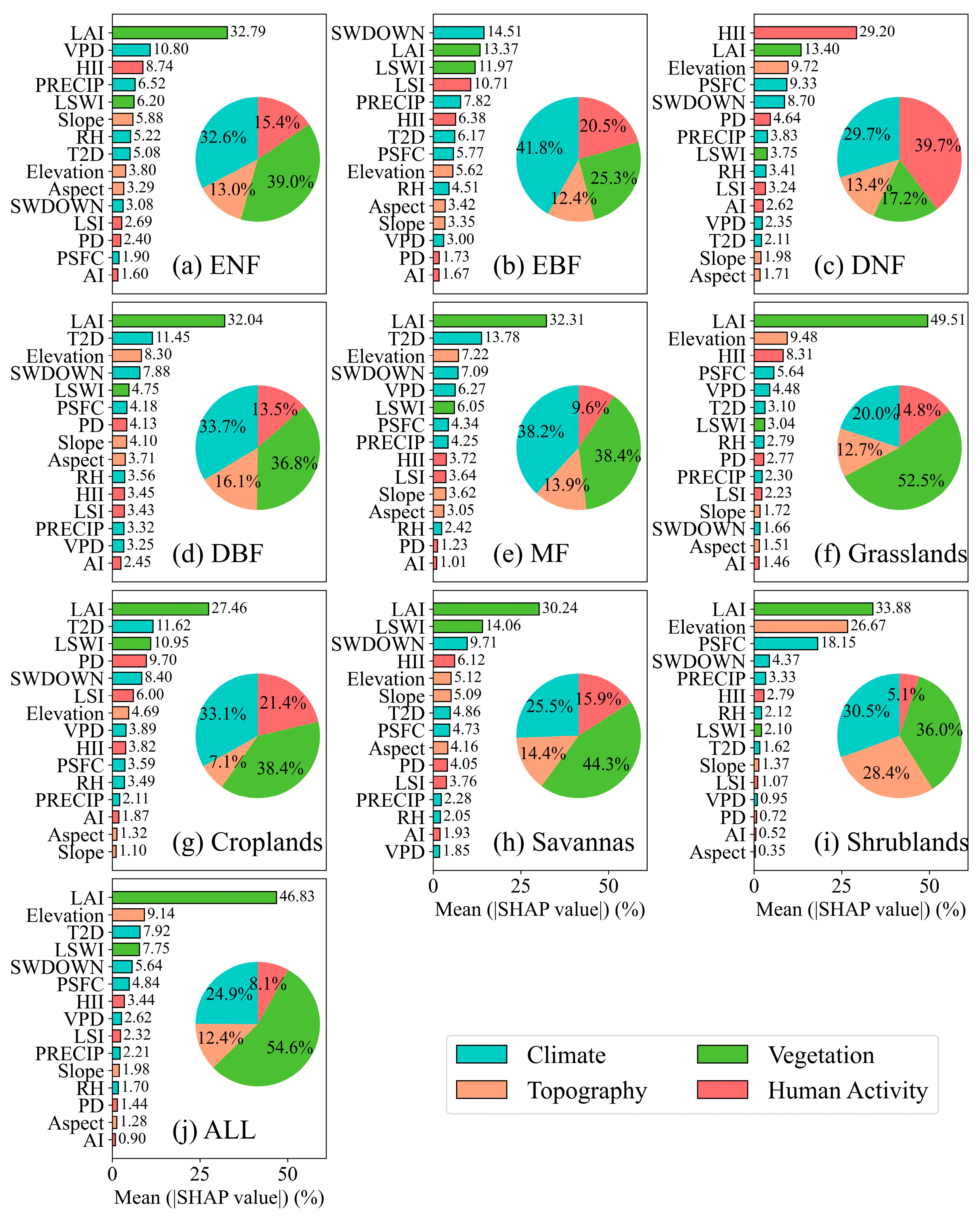
Figure 6 shows the impacts of four types of factors, including climate, vegetation, topography, and human activities, on GPP across different ecosystems. Vegetation factors showed the highest relative importance for modeled GPP, with their mean absolute SHAP values surpassing 25% across all vegetation types except for the DNF ecosystem (Figure 6). In China, the most important predictors of the GPP simulation are LAI, Elevation, T2D, LSWI, and SWDOWN (Figure 6j), reflecting the combined influence of vegetation-related factors (structure, photosynthetic activity, water status) and climate-related factors (radiation and air temperature). When categorized, vegetation factors (54.6%) have the most significant overall impact, followed by climate factors (24.9%), topography (12.4%), and human activities (8.1%) (Figure 6j). However, the factors most strongly associated with GPP vary markedly across ecosystems. In several forest types (i.e., ENF, DBF, MF, and Savannas), as well as in grasslands, croplands, and shrublands, vegetation factors contribute more than 35% (Figure 6a,d–i), underscoring their high relative importance in the model for these ecosystems. Among these vegetation-related variables, LAI emerges as the most strongly associated with GPP variability, particularly in grassland ecosystems, where its contribution reaches 49.51% (Figure 6f). This is because LAI directly determines the surface area available for photosynthesis. In EBF, both climatic factors (i.e., SWDOWN) and vegetation factors (i.e., LAI and LSWI) exert strong influences, highlighting the dual role of energy input and vegetation status in regulating GPP (Figure 6b). In contrast, GPP in DNF is primarily influenced by human activities (39.7%), followed by climatic factors (29.7%), with HII contributing the largest proportion among human activity indicators (Figure 6c). This likely reflects the sensitivity of cold-temperate deciduous needleleaf forests to macro-scale cumulative anthropogenic pressure, where historical logging, forest management, and infrastructure development have shaped forest structure and regeneration patterns, thereby modulating GPP across the landscape.
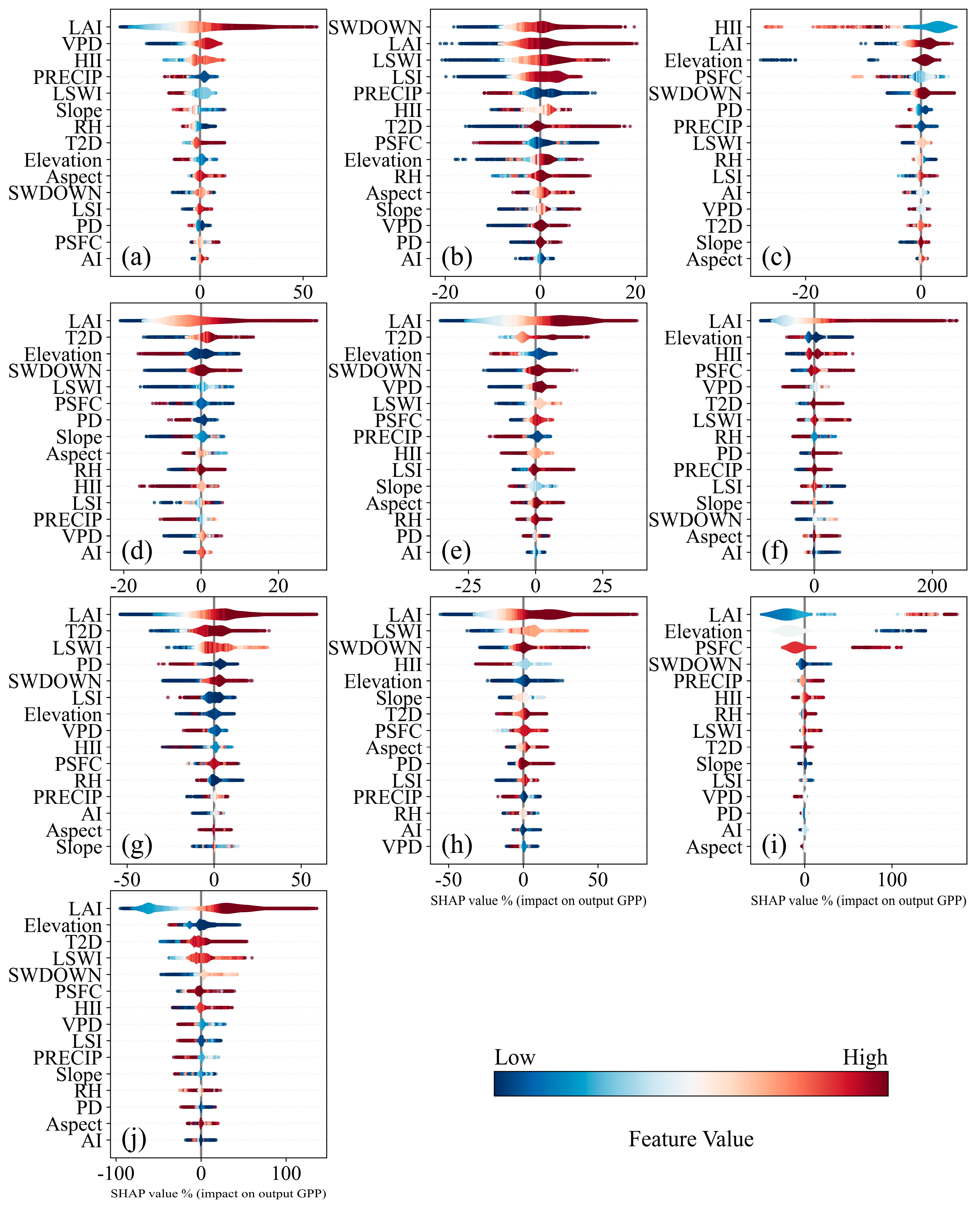
Figure 7 illustrates the relationships between GPP and the four types of influencing factors. Positive SHAP values indicate factors that enhance GPP, thereby identifying key promoters of photosynthesis, while negative values denote suppressive effects. In China, the SHAP violin plots clearly show the model-derived features that are most strongly associated with GPP (Figure 7j). LAI, T2D, LSWI, and SWDOWN are predominantly distributed on the positive side, with high feature values consistently associated with large positive SHAP values, confirming their strong positive influence on photosynthesis. In contrast, VPD exhibits a highly asymmetric pattern: low VPD has minimal impact, whereas high VPD is concentrated in the negative SHAP region, highlighting its role as a physiological stressor that suppresses GPP under arid conditions. Meanwhile, the narrow SHAP ranges for slope, relative humidity, and landscape indices (i.e., PD, AI) indicate their weaker contributions to the model output. Across diverse vegetation ecosystems, LAI consistently emerges as the most influential positive factor of GPP. The SHAP dependence plots for each vegetation type (Figures S2–S11) unequivocally demonstrate strong, near-monotonic positive relationships between these variables and GPP. SWDOWN generally has a positive effect, except in shrublands, where water scarcity likely constrains photosynthetic activity even under high radiation. In the DNF ecosystem, HII exerts the strongest influence on GPP, with low to moderate values contributing positively, while high values suppress GPP. This reflects the influence of macro-scale cumulative anthropogenic pressure [65]. Additionally, the violin plots and SHAP dependence plots reveal the nonlinear responses of climatic and hydrological factors (Figure 7). For VPD and PRECIP, the symmetric or bimodal SHAP distributions indicate context-dependent effects: moderate conditions generally promote or maintain GPP, whereas extreme values drive negative SHAP responses (Moderate feature values correspond to higher SHAP values), reflecting suppression under stress (Figure 7j). A comparable bidirectional pattern is observed for LSWI. The distributions of human activity indices (HII, PD, LSI, AI) show that most areas experience low to moderate disturbance, while areas with high anthropogenic pressure are less common and strongly reduce GPP. In contrast, the compact distributions of topographic variables such as elevation and slope indicate their limited influence on the spatial variation of GPP.
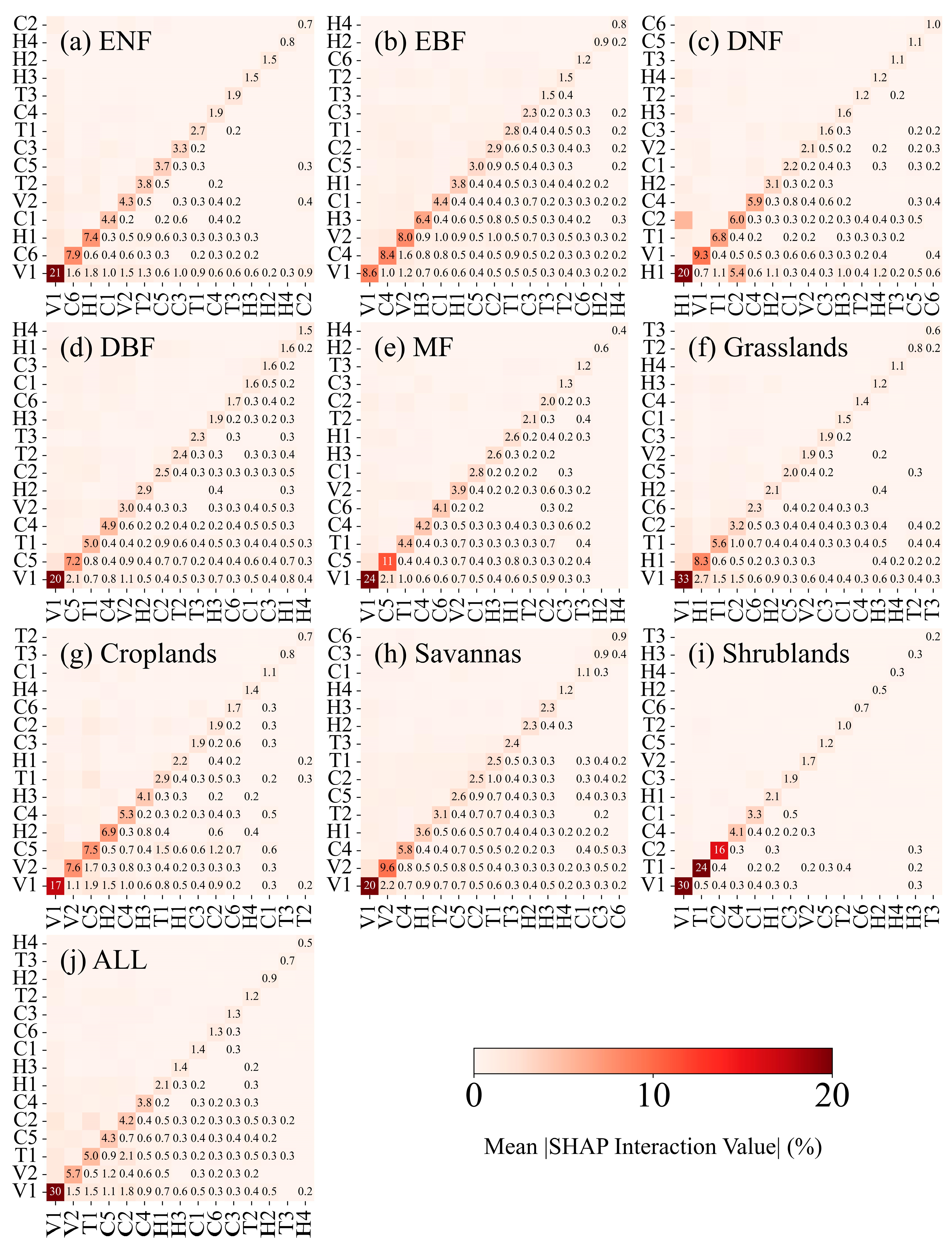
This study further quantified how factor interactions influence the spatiotemporal dynamics of GPP, as shown in Figure 8. GPP variations arise from the coupled effects of vegetation, climate, topography, and human activity. Vegetation factors consistently exhibit strong individual and interactive influence. Notably, the magnitude of certain two-way interactions rivals or exceeds that of individual factor contributions, underscoring the non-linear and synergistic nature of ecosystem productivity controls. This confirms the imperative of incorporating multi-factor coupling in productivity modelling and attribution. In China, LAI is identified as the most important individual feature and the central hub of interaction effects. Among all pairwise interactions, the one between PSFC and elevation is the most pronounced (2.1%) (Figure 8j), underscoring the synergistic influence of topography in modulating near-surface energy and material distributions that collectively affect photosynthetic processes. The interactions between LAI and PSFC (1.8%) as well as between LAI and elevation (1.5%) further highlight the canopy’s sensitivity to topography–climate coupling. Meanwhile, the interaction between LAI and LSWI (1.5%) emphasizes the regulatory role of vegetation water status in canopy functioning. Notably, the interaction between LSWI and T2D (1.2%) reveals an ecological pathway through which temperature influences photosynthetic efficiency by modulating vegetation water stress. Collectively, these interactions delineate a “topography–climate–vegetation” triadic coupling framework that governs the carbon sink dynamics of terrestrial ecosystems across China. The composition and strength of these interactions vary markedly across ecosystem types, revealing distinct regulatory regimes. Forest ecosystems (e.g., ENF, EBF) are characterized by strong climate–vegetation interactions (Figure 8a,b). In DBF, most main effects are relatively weak, whereas the interaction between SWDOWN and LSWI is particularly strong (1.6%), indicating that GPP in this ecosystem is highly sensitive to coupled light–water dynamics. In DNF, a strong HII–PSFC interaction reflects the spatial co-dependence of human activity and topography (Figure 8d). While PSFC varies little over time, it captures spatial gradients that modulate anthropogenic effects on GPP, with stronger effects in low-lying, high-pressure areas and weaker effects at high elevations. Thus, PSFC likely serves as a proxy for terrain-related spatial heterogeneity rather than a direct biophysical driver. No significant HII–Elevation interaction was observed, probably because PSFC represents the same topographic gradient as elevation but aligns more closely with human activity intensity, making it a more effective indicator of terrain-mediated anthropogenic impacts on GPP (Figure S1).
In grassland and cropland ecosystems, GPP shows the strongest associations with LAI. In grasslands, the interaction between LAI and HII reflects how cumulative human pressures modulate canopy structure and productivity, without resolving specific management activities. Interactions of LAI with elevation and surface pressure indicate the indirect effects of topography on canopy functioning via hydrothermal conditions (Figure 8f). In croplands, the interactions among PD, T2D, and LSWI collectively capture the synergistic regulation of landscape structure, climatic conditions, and aggregated human influence on vegetation water status and canopy functioning (Figure 8g). These results suggest that although LAI plays a central role in both ecosystems, grassland GPP is jointly influenced by direct human disturbances and indirect topographic regulation, whereas cropland GPP is primarily governed by the interaction between intensive management and environmental factors. In contrast, the relatively weak interaction strengths observed in savannas and shrublands (Figure 8h,i) may be attributed to their simpler structure–function relationships or more homogeneous environmental controls.

4. Discussion

4.1. Combined Effects of Vegetation and Climatic Factors on GPP

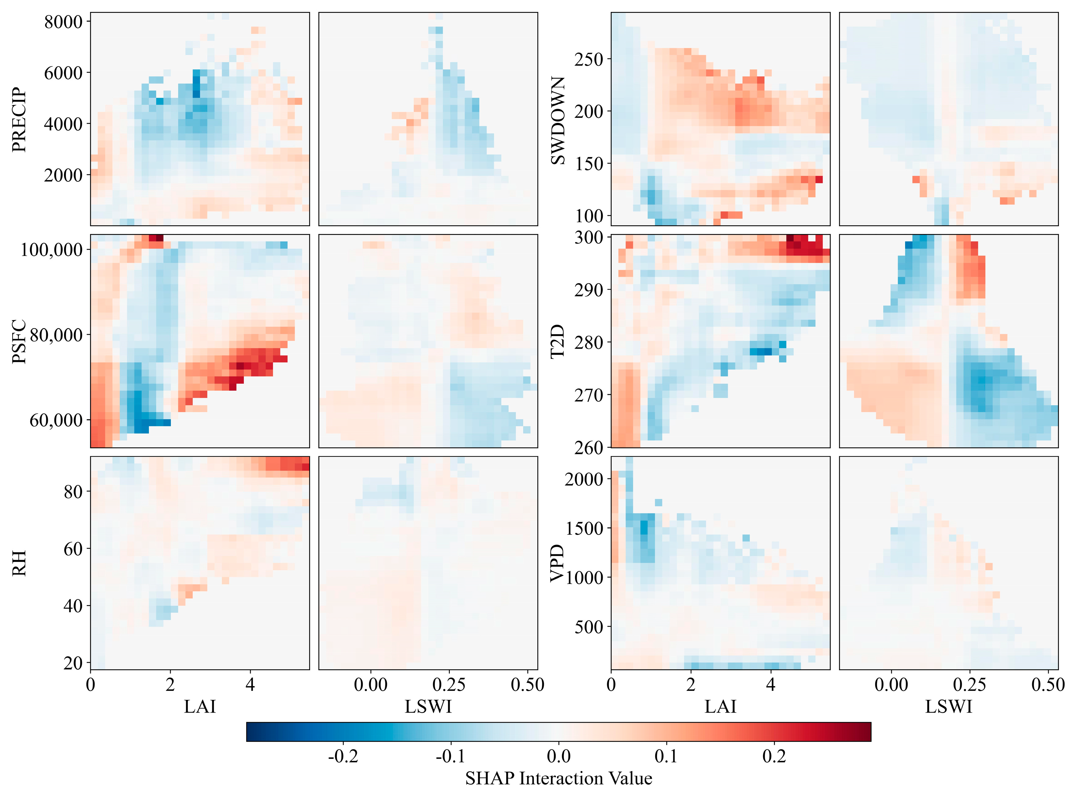
Our analysis indicates that vegetation structure, notably LAI, is most strongly associated with GPP variability across ecosystems, consistent with its role as a key proxy for canopy photosynthetic capacity [66]. However, the extent to which this potential is realized appears to be contingent on ambient environmental conditions [67,68,69]. The SHAP interaction results demonstrate that modeled GPP patterns are associated not with isolated factors alone, but with their combined and often nonlinear interactions [70], in which climatic and hydrological variables condition the expression of vegetation-related signals (Figure 9). This synergistic pattern manifests through several key mechanisms. First, the influence of LAI, while universally positive, exhibits pronounced environmental contingency [71,72]. It acts as a crucial buffer under abiotic stress, sustaining productivity during drought and under low light [73], whereas under benign conditions, the system becomes less dependent on dense canopy (large LAI). Second, the interplay between air temperature (T2D) and vegetation water status (LSWI) is pivotal: GPP peaks when both are high, but this synergy fractures under mismatched conditions, inducing drought stress or metabolic limitation [74]. Finally, at the physiological level, the interaction between LAI and SWDOWN reflects the principle of resource co-limitation: GPP reaches its maximum only when both sufficient canopy light-capturing capacity (high LAI) and abundant solar radiation (high SWDOWN) are present [75,76].
This framework of synergistic control is robust across ecosystems, yet it manifests through distinct pathways shaped by vegetation structure and environmental constraints, as detailed in our ecosystem-specific analysis (Figures S12–S20) [77]. For instance, forests exhibit strong coupling between canopy structure (LAI) and climatic drivers like VPD and radiation, highlighting the role of canopy-mediated resource regulation [78]. In contrast, the productivity of grasslands and shrublands shows weaker climate-vegetation interactions, suggesting simpler regulatory mechanisms [79]. Meanwhile, agricultural ecosystems exhibit high sensitivity of LAI to temperature and light. This phenomenon can be attributed to human management practices (e.g., irrigation and fertilization), which modulate water and nutrient availability, making crop productivity more sensitive to the interactions between canopy structure (LAI) and environmental factors such as temperature and light, rather than being solely dominated by climatic drivers [80,81].
In summary, our findings highlight that ecosystem productivity emerges from the complex interplay of biophysical processes rather than from isolated environmental controls. The influences of canopy structure, photosynthetic function, temperature, and water status are intrinsically interconnected [82]. Disentangling these factors without considering their mutual feedback risks misrepresenting the true drivers of carbon flux, particularly under extreme climatic conditions where nonlinear interactions are most pronounced. Incorporating such mechanistic and synergistic processes into terrestrial biosphere models is therefore essential to reduce uncertainties in simulating and projecting the global carbon cycle [83].

4.2. Combined Effects of Human Activity and Landscape Fragmentation on GPP

Human activities exert multifaceted impacts on GPP by altering land-use intensity, landscape configuration, and overall disturbance regimes [84]. In this study, human impacts are represented by the HII, which captures spatial gradients of aggregated anthropogenic pressure rather than specific management actions.
SHAP analysis indicates that HII explains a larger proportion of GPP variability than natural drivers in DNF (Figure 7c). Although DNF ecosystems in Northeast China, particularly in the Greater Khingan Mountains, are characterized by relatively low population density and limited urban development, human disturbance exhibits pronounced spatial heterogeneity due to historical logging, forest management, transportation infrastructure, and fire-control activities. Under the region’s cold climate and short growing season, climatic constraints on productivity are relatively uniform, whereas variations in cumulative human pressure strongly modulate forest structure, regeneration status, and carbon uptake capacity. As a result, GPP variability in these forests is more sensitive to anthropogenic disturbance gradients than to short-term climatic fluctuations [85]. This dominant role of HII therefore reflects the high sensitivity of cold-temperate forests to cumulative disturbance legacies, rather than the intensity of contemporary human activities per se.
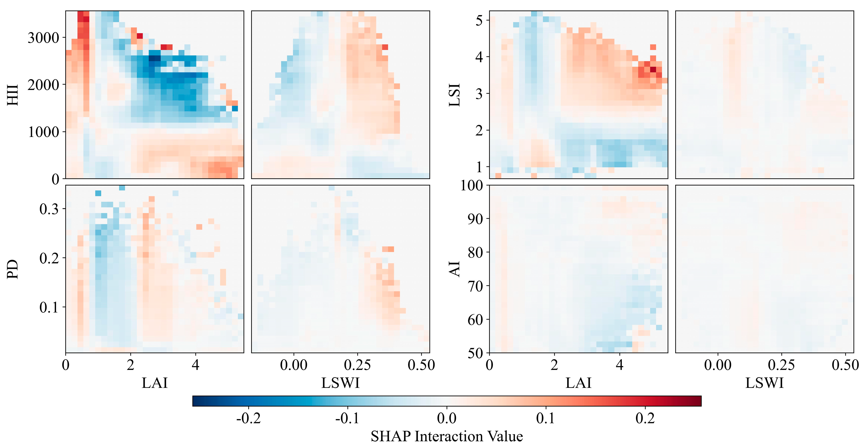
SHAP dependence analysis further reveals that combinations of high HII and high LAI are associated with negative contributions to GPP, suggesting that strong cumulative human pressure may offset the productivity advantages of dense canopies, potentially through long-term alterations of stand structure or microenvironmental conditions. In contrast, positive SHAP responses occur under low LAI–high HII or high LAI–low HII conditions (Figure 10), highlighting the strong context dependence of anthropogenic effects on ecosystem productivity. Importantly, these patterns should be interpreted as statistical associations with aggregated disturbance intensity, rather than direct evidence of specific human activities [86,87].
Moreover, SHAP interaction analysis reveals a pronounced nonlinear coupling between HII and PSFC (Figure 8c), indicating that the effects of cumulative human pressure on GPP are strongly modulated by atmospheric conditions. Under relatively favorable conditions, moderate levels of aggregated human influence may coincide with enhanced productivity, whereas in climatically constrained or environmentally fragile settings, intensified disturbance tends to suppress GPP, underscoring the vulnerability of stressed ecosystems to cumulative pressure.
In addition to anthropogenic influence, landscape configuration, quantified by indices such as LSI and PD, plays a critical role in ecosystem functioning. Landscape fragmentation disrupts the exchange of energy, water, and nutrients among patches, weakens ecological connectivity, and constrains overall productivity [88]. Together, these results demonstrate that GPP dynamics emerge from the combined effects of cumulative human pressure, spatial structure, and vegetation traits, emphasizing the importance of considering anthropogenic–landscape interactions when assessing terrestrial carbon-cycle dynamics [89].

4.3. Implications for Ecosystem Management and Climate Adaptation

The spatio-temporal patterns of GPP across China highlight that ecosystem productivity is governed by complex, nonlinear interactions among vegetation, climate, topography, and human activities. These interactions are highly ecosystem-specific, indicating that uniform management or restoration strategies are unlikely to be effective. In forest ecosystems, for instance, GPP is strongly influenced by the coupling between canopy structure, represented by LAI, and climatic factors such as solar radiation and temperature [90]. This suggests that maintaining forest canopy integrity and promoting natural regeneration while accounting for climate–vegetation interactions are critical for sustaining carbon sequestration. Grassland productivity is more sensitive to topographic constraints and aggregated human disturbance, suggesting that restoration efforts should focus on maintaining soil–water balance, reducing excessive disturbance, and accounting for terrain-induced microclimatic variability [28]. In croplands, GPP is strongly regulated by the interaction between climatic conditions and management-related anthropogenic influence, as reflected by landscape structure and vegetation water status, highlighting the importance of climate-adaptive and resource-efficient agricultural management for sustaining productivity and carbon sequestration [84,89].
Incorporating these nonlinear and ecosystem-dependent interactions into carbon cycle models can improve predictions of ecosystem responses to climate change, thereby supporting climate-adaptive land-use planning [91]. Regions exhibiting rapid GPP increases, such as Northeast, North, and Central South China, may benefit from conservation and climate-smart management to sustain carbon gains, whereas areas with slower growth, particularly the arid Northwest, require strategies to enhance ecosystem resilience, including targeted vegetation restoration, water management, and mitigation of anthropogenic pressures. Furthermore, understanding the role of cumulative human influence, as captured by the Human Influence Index, provides a basis for implementing targeted interventions such as landscape planning, regulation of intensive land use, and monitoring of human activities to optimize ecosystem productivity.
Overall, these findings emphasize that ecosystem management and climate adaptation policies must consider the interactive, ecosystem-specific drivers of productivity. By integrating ecological, climatic, and human dimensions, management strategies can more effectively enhance carbon sequestration, improve ecosystem resilience, and support sustainable land-use planning at national and regional scales.

4.4. Limitations and Future Perspectives

To ensure consistency across multi-source datasets in terms of spatial resolution, all data in this study were resampled to 0.1°. However, this processing may introduce uncertainties, particularly in areas with high ecological heterogeneity, as spatial aggregation can obscure local ecological differences and cause scale-dependent biases. Previous studies have shown that spatial upscaling can smooth local extremes, reduce variance, and alter statistical relationships between ecosystem variables, a phenomenon commonly referred to as scale or aggregation effects [92,93]. These effects are especially relevant for landscape metrics such as PD and LSI, which are inherently sensitive to spatial resolution and grain size. Aggregation to coarser resolutions may underestimate landscape fragmentation by merging small patches, simplifying patch boundaries, and reducing edge complexity, thereby weakening the apparent influence of landscape configuration on ecosystem processes [94,95,96]. Similarly, in regions with strong environmental heterogeneity, resampling may dampen localized human disturbances or microclimatic gradients, potentially leading to conservative estimates of their impacts on GPP. Despite these limitations, the 0.1° resolution adopted here represents a compromise between computational feasibility, data availability, and the need to capture large-scale spatial patterns at the national scale. The observed relationships should therefore be interpreted as macro-scale associations, rather than fine-scale process-level mechanisms. Future studies could reduce this uncertainty by conducting multi-resolution analyses or integrating higher-resolution datasets to explicitly assess scale dependence and cross-scale interactions in carbon-cycle dynamics.
This study focuses on aboveground GPP and does not explicitly account for belowground carbon pools, such as soil carbon sequestration, which may contribute substantially to cumulative ecosystem carbon dynamics. In addition, human impacts are represented by the Human Influence Index (HII), a composite metric that aggregates multiple anthropogenic pressures including population density, land use, transportation infrastructure, and accessibility. While HII effectively captures macro-scale gradients of human disturbance, it cannot resolve individual management activities such as timber harvesting, grazing, irrigation, or temporal changes in population and land use intensity, which can strongly modulate GPP in forests, grasslands, and croplands. Therefore, the observed relationships between HII and GPP should be interpreted as associations with cumulative anthropogenic pressure, rather than the effects of specific human actions. Future research could combine HII with finer-scale or activity-specific datasets to disentangle the contributions of individual human activities to ecosystem productivity [97,98].
Moreover, land management practices (e.g., forest and agricultural management) and local regulatory policies were not explicitly considered in this study. Incorporating these factors in future analyses could provide more precise assessments of their influence on ecosystem productivity and carbon dynamics, particularly at regional and local scales.
Overall, while our study provides robust insights into national-scale GPP patterns and their drivers, these limitations highlight the need for future research integrating multi-scale, multi-source datasets and explicit consideration of understory carbon pools, anthropogenic interventions, and land management practices to fully understand ecosystem carbon dynamics in China.

5. Conclusions

This study provides a comprehensive assessment of the spatio-temporal dynamics of ecosystem GPP across China from 2001 to 2020, and explores the factors associated with GPP variability using SHAP−based interpretable machine learning. Notably, examining the interactions among climate, environment, topography, and human activity factors and their associations with GPP represents a key methodological contribution of this study. The main conclusions are as follows:
Nationwide, GPP exhibited a significant upward trend, with the most pronounced increases observed in DBF, croplands, grasslands, and savannas, particularly during the growing season, highlighting the heterogeneous enhancement of ecosystem productivity across vegetation types.
SHAP analysis suggests that LAI is the most influential factor associated with GPP, reflecting its potential role in determining canopy photosynthetic capacity. Climatic factors, including radiation, temperature, and water availability, are associated with GPP through nonlinear interactions rather than isolated effects. Interaction analyses further indicate that vegetation factors, particularly LAI, are strongly linked to GPP and appear to mediate relationships with climate, topography, and human activity factors. For example, the coupling between LAI and SWDOWN affects GPP by mediating the co-limitation of light capture and carbon fixation, while T2D and LSWI jointly correspond to variations in GPP related to temperature and water availability.
These interactions exhibit pronounced ecosystem-specific heterogeneity in driving GPP. Forest GPP shows strong association with climate–vegetation coupling (SWDOWN × LSWI), and human–topographic (HII × PSFC) interactions are associated with variation in GPP, where anthropogenic influence and terrain are jointly linked to productivity patterns. Although LAI is the factor most strongly associated with GPP in both grasslands and croplands, grassland GPP is additionally influenced by the combined effects of human disturbance and topographic regulation, whereas cropland GPP is predominantly associated with the combined effects of landscape management (PD) and hydrothermal conditions (T2D × LSWI). The weaker interactions observed in GPP of savannas and shrublands likely indicate simpler environment–vegetation associations.
Human activities exert context-dependent effects on GPP: moderate management practices, such as irrigation and fertilization, enhance productivity, whereas intensive disturbances exert suppressive effects. Overall, these findings demonstrate that GPP dynamics across China are governed by multidimensional synergies within a coupled topography–climate–vegetation–human framework. Incorporating such nonlinear interaction mechanisms into carbon cycle models is critical for reducing structural uncertainty and improving projections of ecosystem productivity. Importantly, these insights provide a scientific basis for ecosystem-specific restoration and conservation strategies, adaptive management under climate change, and more realistic assessments of regional carbon sequestration potential.

Supplementary Materials

The following supporting information can be downloaded at: https://www.mdpi.com/article/10.3390/rs18020275/s1, Figure S1: SHAP interaction between HII and PSFC and its relationship with elevation. (a) Heatmap of SHAP interaction values between HII and PSFC. (b) Scatter plot showing the relationship between PSFC and elevation; Figure S2: SHAP dependence plots showing the marginal effects of individual predictors on GPP in the ENF ecosystem; Figure S3: SHAP dependence plots showing the marginal effects of individual predictors on GPP in the EBF ecosystem; Figure S4: SHAP dependence plots showing the marginal effects of individual predictors on GPP in the DNF ecosystem; Figure S5: SHAP dependence plots showing the marginal effects of individual predictors on GPP in the DBF ecosystem; Figure S6: SHAP dependence plots showing the marginal effects of individual predictors on GPP in the MF ecosystem; Figure S7: SHAP dependence plots showing the marginal effects of individual predictors on GPP in the Grasslands ecosystem; Figure S8: SHAP dependence plots showing the marginal effects of individual predictors on GPP in the Croplands ecosystem; Figure S9: SHAP dependence plots showing the marginal effects of individual predictors on GPP in the Savannas ecosystem; Figure S10: SHAP dependence plots showing the marginal effects of individual predictors on GPP in the Shrublands ecosystem; Figure S11: SHAP dependence plots showing the marginal effects of individual predictors on GPP across all ecosystems; Figure S12: SHAP Interaction heatmap of vegetation and climatic variables in the ENF ecosystem; Figure S13: SHAP Interaction heatmap of vegetation and climatic variables in the EBF ecosystem; Figure S14: SHAP Interaction heatmap of vegetation and climatic variables in the DNF ecosystem; Figure S15: SHAP Interaction heatmap of vegetation and climatic variables in the DBF ecosystem; Figure S16: SHAP Interaction heatmap of vegetation and climatic variables in the MF ecosystem; Figure S17: SHAP Interaction heatmap of vegetation and climatic variables in the Grasslands ecosystem; Figure S18: SHAP Interaction heatmap of vegetation and climatic variables in the Croplands ecosystem; Figure S19: SHAP Interaction heatmap of vegetation and climatic variables in the Savannas ecosystem; Figure S20. SHAP Interaction heatmap of vegetation and climatic variables in the Shrublands ecosystem; Table S1: Abbreviations and full names used in this study; Table S2: Cross-validation and evaluation metrics of optimal XGBoost models across vegetation types; Table S3: Optimal hyperparameters of XGBoost models for different vegetation types. The hyperparameters were tuned using FLAML, with the optimal configuration determined based on the highest R2.

Author Contributions

Conceptualization: Y.D., J.L., and W.F.; Data processing and analysis: J.L.; writing—original draft preparation: J.L., L.H., and W.F.; writing—review and editing: Y.D., A.W., J.W., Y.L., L.S., Y.Z., R.C., and H.Z.; supervision: W.F. and H.Z.; Funding: Y.D. and W.F. All authors have read and agreed to the published version of the manuscript.

Funding

This work was supported by the Open Research Fund Project of Key Laboratory of Ecosystem Carbon Source and Sink, China Meteorological Administration (Grant Number: ECSS-CMA202305), the National Natural Science Foundation of China (Grant Number: 32401667), and the Natural Science Foundation of Liaoning Province (2024-BSBA-62).

Data Availability Statement

The original data presented in the study are openly available from the following publicly accessible sources: The Penman−Monteith–Leuning Version 2 (PML−V2) (China) terrestrial GPP dataset at https://data.tpdc.ac.cn/en/data/40f57c67-33a6-402d-bd37-6ede91919f23/; MODIS MCD12Q1 land cover dataset at https://developers.google.com/earth-engine/datasets/catalog/MODIS_061_MCD12Q1; MODIS MOD09A1 surface reflectance dataset at https://ladsweb.modaps.eosdis.nasa.gov/missions-and-measurements/products/MOD09A1; CMFD dataset at https://www.tpdc.ac.cn/zh-hans/data/e60dfd96-5fd8-493f-beae-e8e5d24dece4; GLASS LAI dataset at https://glass-product.bnu.edu.cn/introduction1/LAI.html; SRTM DEM dataset at https://doi.org/10.5067/MEASURES/SRTM/SRTMGL1.003; WCS HII dataset at https://www.wcshumanfootprint.org/data-access (accessed on 5 January 2026).

Conflicts of Interest

The authors declare no conflicts of interest.

References

  1. Beer, C.; Reichstein, M.; Tomelleri, E.; Ciais, P.; Jung, M.; Carvalhais, N.; Rödenbeck, C.; Arain, M.A.; Baldocchi, D.; Bonan, G.B.; et al. Terrestrial Gross Carbon Dioxide Uptake: Global Distribution and Covariation with Climate. Science 2010, 329, 834–838. [Google Scholar] [CrossRef] [PubMed]
  2. Chapin, F.S.; Matson, P.A.; Mooney, H. Principles of Terrestrial Ecosystem Eology; Springer: New York, NY, USA, 2002; ISBN 978-1-4419-9503-2. [Google Scholar]
  3. Friedlingstein, P.; O’Sullivan, M.; Jones, M.W.; Andrew, R.M.; Gregor, L.; Hauck, J.; Le Quéré, C.; Luijkx, I.T.; Olsen, A.; Peters, G.P.; et al. Global Carbon Budget 2022. Earth Syst. Sci. Data 2022, 14, 4811–4900. [Google Scholar] [CrossRef]
  4. Schimel, D.; Stephens, B.B.; Fisher, J.B. Effect of Increasing CO2 on the Terrestrial Carbon Cycle. Proc. Natl. Acad. Sci. USA 2015, 112, 436–441. [Google Scholar] [CrossRef]
  5. Andersson, K.; Evans, T.P.; Richards, K.R. National Forest Carbon Inventories: Policy Needs and Assessment Capacity. Clim. Change 2009, 93, 69–101. [Google Scholar] [CrossRef]
  6. Canadell, J.G.; Mooney, H.A.; Baldocchi, D.D.; Berry, J.A.; Ehleringer, J.R.; Field, C.B.; Gower, S.T.; Hollinger, D.Y.; Hunt, J.E.; Jackson, R.B.; et al. Commentary: Carbon Metabolism of the Terrestrial Biosphere: A Multitechnique Approach for Improved Understanding. Ecosystems 2000, 3, 115–130. [Google Scholar] [CrossRef]
  7. Anav, A.; Friedlingstein, P.; Beer, C.; Ciais, P.; Harper, A.; Jones, C.; Murray-Tortarolo, G.; Papale, D.; Parazoo, N.C.; Peylin, P.; et al. Spatiotemporal Patterns of Terrestrial Gross Primary Production: A Review. Rev. Geophys. 2015, 53, 785–818. [Google Scholar] [CrossRef]
  8. Zhao, M.; Running, S.W. Drought-Induced Reduction in Global Terrestrial Net Primary Production from 2000 Through 2009. Science 2010, 329, 940–943. [Google Scholar] [CrossRef]
  9. Piao, S.; Friedlingstein, P.; Ciais, P.; Viovy, N.; Demarty, J. Growing Season Extension and Its Impact on Terrestrial Carbon Cycle in the Northern Hemisphere over the Past 2 Decades. Global Biogeochem. Cycles 2007, 21, GB3018. [Google Scholar] [CrossRef]
  10. Piao, S.; Nan, H.; Huntingford, C.; Ciais, P.; Friedlingstein, P.; Sitch, S.; Peng, S.; Ahlström, A.; Canadell, J.G.; Cong, N.; et al. Evidence for a Weakening Relationship between Interannual Temperature Variability and Northern Vegetation Activity. Nat. Commun. 2014, 5, 5018. [Google Scholar] [CrossRef] [PubMed]
  11. Yuan, W.; Cai, W.; Chen, Y.; Liu, S.; Dong, W.; Zhang, H.; Yu, G.; Chen, Z.; He, H.; Guo, W.; et al. Severe Summer Heatwave and Drought Strongly Reduced Carbon Uptake in Southern China. Sci. Rep. 2016, 6, 18813. [Google Scholar] [CrossRef]
  12. Piao, S.; Tan, K.; Nan, H.; Ciais, P.; Fang, J.; Wang, T.; Vuichard, N.; Zhu, B. Impacts of Climate and CO2 Changes on the Vegetation Growth and Carbon Balance of Qinghai–Tibetan Grasslands over the Past Five Decades. Glob. Planet. Change 2012, 98–99, 73–80. [Google Scholar] [CrossRef]
  13. Bo, Y.; Li, X.; Liu, K.; Wang, S.; Zhang, H.; Gao, X.; Zhang, X. Three Decades of Gross Primary Production (GPP) in China: Variations, Trends, Attributions, and Prediction Inferred from Multiple Datasets and Time Series Modeling. Remote Sens. 2022, 14, 2564. [Google Scholar] [CrossRef]
  14. Li, X.; Zhu, Z.; Zeng, H.; Piao, S. Estimation of Gross Primary Production in China (1982–2010) with Multiple Ecosystem Models. Ecol. Model. 2016, 324, 33–44. [Google Scholar] [CrossRef]
  15. Xie, S.; Mo, X.; Hu, S.; Liu, S. Contributions of Climate Change, Elevated Atmospheric CO2 and Human Activities to ET and GPP Trends in the Three-North Region of China. Agric. For. Meteorol. 2020, 295, 108183. [Google Scholar] [CrossRef]
  16. Zhang, Y.; Song, C.; Zhang, K.; Cheng, X.; Zhang, Q. Spatial–Temporal Variability of Terrestrial Vegetation Productivity in the Yangtze River Basin during 2000–2009. J. Plant Ecol. 2014, 7, 10–23. [Google Scholar] [CrossRef]
  17. Ge, W.; Han, J.; Zhang, D.; Wang, F. Divergent Impacts of Droughts on Vegetation Phenology and Productivity in the Yungui Plateau, Southwest China. Ecol. Indic. 2021, 127, 107743. [Google Scholar] [CrossRef]
  18. Piao, S.; Ciais, P.; Huang, Y.; Shen, Z.; Peng, S.; Li, J.; Zhou, L.; Liu, H.; Ma, Y.; Ding, Y.; et al. The Impacts of Climate Change on Water Resources and Agriculture in China. Nature 2010, 467, 43–51. [Google Scholar] [CrossRef] [PubMed]
  19. Zhou, H.; Yue, X.; Wang, B.; Tian, C.; Lu, X.; Zhu, J.; Cao, Y. Distinguishing the Main Climatic Drivers to the Variability of Gross Primary Productivity at Global FLUXNET Sites. Environ. Res. Lett. 2023, 18, 124007. [Google Scholar] [CrossRef]
  20. Piao, S.; Ciais, P.; Lomas, M.; Beer, C.; Liu, H.; Fang, J.; Friedlingstein, P.; Huang, Y.; Muraoka, H.; Son, Y.; et al. Contribution of Climate Change and Rising CO2 to Terrestrial Carbon Balance in East Asia: A Multi-Model Analysis. Glob. Planet. Change 2011, 75, 133–142. [Google Scholar] [CrossRef]
  21. Khalifa, M.; Elagib, N.A.; Ribbe, L.; Schneider, K. Spatio-Temporal Variations in Climate, Primary Productivity and Efficiency of Water and Carbon Use of the Land Cover Types in Sudan and Ethiopia. Sci. Total Environ. 2018, 624, 790–806. [Google Scholar] [CrossRef] [PubMed]
  22. Zhu, W.; Pan, Y.; Yang, X.; Song, G. Comprehensive Analysis of the Impact of Climatic Changes on Chinese Terrestrial Net Primary Productivity. Chin. Sci. Bull. 2007, 52, 3253–3260. [Google Scholar] [CrossRef]
  23. Yue, X.; Unger, N.; Zheng, Y. Distinguishing the Drivers of Trends in Land Carbon Fluxes and Plant Volatile Emissions over the Past 3 Decades. Atmos. Chem. Phys. 2015, 15, 11931–11948. [Google Scholar] [CrossRef]
  24. Ciais, P.; Reichstein, M.; Viovy, N.; Granier, A.; Ogée, J.; Allard, V.; Aubinet, M.; Buchmann, N.; Bernhofer, C.; Carrara, A.; et al. Europe-Wide Reduction in Primary Productivity Caused by the Heat and Drought in 2003. Nature 2005, 437, 529–533. [Google Scholar] [CrossRef]
  25. Chen, Y.; Feng, X.; Tian, H.; Wu, X.; Gao, Z.; Feng, Y.; Piao, S.; Lv, N.; Pan, N.; Fu, B. Accelerated Increase in Vegetation Carbon Sequestration in China after 2010: A Turning Point Resulting from Climate and Human Interaction. Glob. Change Biol. 2021, 27, 5848–5864. [Google Scholar] [CrossRef] [PubMed]
  26. Naeem, S.; Zhang, Y.; Tian, J.; Qamer, F.M.; Latif, A.; Paul, P.K. Quantifying the Impacts of Anthropogenic Activities and Climate Variations on Vegetation Productivity Changes in China from 1985 to 2015. Remote Sens. 2020, 12, 1113. [Google Scholar] [CrossRef]
  27. Liu, X.; Cui, Y.; Li, W.; Li, M.; Li, N.; Shi, Z.; Dong, J.; Xiao, X. Urbanization Expands the Fluctuating Difference in Gross Primary Productivity between Urban and Rural Areas from 2000 to 2018 in China. Sci. Total Environ. 2023, 901, 166490. [Google Scholar] [CrossRef] [PubMed]
  28. Xue, Y.; Liang, H.; Ma, Y.; Xue, G.; He, J. The Impacts of Climate and Human Activities on Grassland Productivity Variation in China. Remote Sens. 2023, 15, 3864. [Google Scholar] [CrossRef]
  29. Luo, L.; Ma, W.; Zhuang, Y.; Zhang, Y.; Yi, S.; Xu, J.; Long, Y.; Ma, D.; Zhang, Z. The Impacts of Climate Change and Human Activities on Alpine Vegetation and Permafrost in the Qinghai-Tibet Engineering Corridor. Ecol. Indic. 2018, 93, 24–35. [Google Scholar] [CrossRef]
  30. Liu, Y.; Liu, H.; Chen, Y.; Gang, C.; Shen, Y. Quantifying the Contributions of Climate Change and Human Activities to Vegetation Dynamic in China Based on Multiple Indices. Sci. Total Environ. 2022, 838, 156553. [Google Scholar] [CrossRef]
  31. Shapley, L.S. A Value for n-Person Games. In Contributions to the Theory of Games, Volume II; Kuhn, H.W., Tucker, A.W., Eds.; Princeton University Press: Princeton, NJ, USA, 1953; pp. 307–318. ISBN 978-1-4008-8197-0. [Google Scholar]
  32. Zhou, H.; Yue, X.; Dai, H.; Geng, G.; Yuan, W.; Chen, J.; Shen, G.; Zhang, T.; Zhu, J.; Liao, H. Recovery of Ecosystem Productivity in China Due to the Clean Air Action Plan. Nat. Geosci. 2024, 17, 1233–1239. [Google Scholar] [CrossRef]
  33. Beck, H.E.; McVicar, T.R.; Vergopolan, N.; Berg, A.; Lutsko, N.J.; Dufour, A.; Zeng, Z.; Jiang, X.; van Dijk, A.I.J.M.; Miralles, D.G. High-Resolution (1 Km) Köppen-Geiger Maps for 1901–2099 Based on Constrained CMIP6 Projections. Sci. Data 2023, 10, 724. [Google Scholar] [CrossRef]
  34. He, S.; Zhang, Y.; Ma, N.; Tian, J.; Kong, D.; Liu, C. A Daily and 500m Coupled Evapotranspiration and Gross Primary Production Product across China during 2000–2020. Earth Syst. Sci. Data 2022, 14, 5463–5488. [Google Scholar] [CrossRef]
  35. Qian, L.; Yu, X.; Zhang, Z.; Wu, L.; Fan, J.; Xiang, Y.; Chen, J.; Liu, X. Assessing and Improving the High Uncertainty of Global Gross Primary Productivity Products Based on Deep Learning under Extreme Climatic Conditions. Sci. Total Environ. 2024, 957, 177344. [Google Scholar] [CrossRef]
  36. Sulla-Menashe, D.; Friedl, M.A. User Guide to Collection 6 MODIS Land Cover (MCD12Q1 and MCD12C1) Product; U.S. Geological Survey: Reston, VA, USA, 2022. [Google Scholar]
  37. Bajgain, R.; Xiao, X.; Basara, J.; Wagle, P.; Zhou, Y.; Zhang, Y.; Mahan, H. Assessing Agricultural Drought in Summer over Oklahoma Mesonet Sites Using the Water-Related Vegetation Index from MODIS. Int. J. Biometeorol. 2017, 61, 377–390. [Google Scholar] [CrossRef]
  38. He, J.; Yang, K.; Tang, W.; Lu, H.; Qin, J.; Chen, Y.; Li, X. The First High-Resolution Meteorological Forcing Dataset for Land Process Studies over China. Sci. Data 2020, 7, 25. [Google Scholar] [CrossRef]
  39. Sun, P.; Wu, S.; Zhang, K.; Wan, M.; Wang, R. A New Global Grid-Based Weighted Mean Temperature Model Considering Vertical Nonlinear Variation. Atmos. Meas. Tech. 2021, 14, 2529–2542. [Google Scholar] [CrossRef]
  40. Zhang, H.; Wu, B.; Yan, N.; Zhu, W.; Feng, X. An Improved Satellite-Based Approach for Estimating Vapor Pressure Deficit from MODIS Data. J. Geophys. Res. Atmos. 2014, 119, 12256–12271. [Google Scholar] [CrossRef]
  41. Xiao, Z.; Liang, S.; Wang, J.; Chen, P.; Yin, X.; Zhang, L.; Song, J. Use of General Regression Neural Networks for Generating the GLASS Leaf Area Index Product from Time-Series MODIS Surface Reflectance. IEEE Trans. Geosci. Remote Sens. 2014, 52, 209–223. [Google Scholar] [CrossRef]
  42. Xiao, Z.; Liang, S.; Jiang, B. Evaluation of Four Long Time-Series Global Leaf Area Index Products. Agric. For. Meteorol. 2017, 246, 218–230. [Google Scholar] [CrossRef]
  43. Xu, B.; Li, J.; Park, T.; Liu, Q.; Zeng, Y.; Yin, G.; Zhao, J.; Fan, W.; Yang, L.; Knyazikhin, Y.; et al. An Integrated Method for Validating Long-Term Leaf Area Index Products Using Global Networks of Site-Based Measurements. Remote Sens. Environ. 2018, 209, 134–151. [Google Scholar] [CrossRef]
  44. Liu, X.; Ran, M.; Xia, H.; Deng, M. Evaluating Vertical Accuracies of Open-Source Digital Elevation Models over Multiple Sites in China Using GPS Control Points. Remote Sens. 2022, 14, 2000. [Google Scholar] [CrossRef]
  45. Sanderson, E.W.; Fisher, K.; Robinson, N.; Sampson, D.; Duncan, A.; Royte, L. The March of the Human Footprint. EcoEvoRxiv Preprint 2022. [Google Scholar] [CrossRef]
  46. Wang, X.; Hao, J.-Q.; Dai, Z.-Z.; Haider, S.; Chang, S.; Zhu, Z.-Y.; Duan, J.; Ren, G.-X. Spatial-Temporal Characteristics of Cropland Distribution and Its Landscape Fragmentation in China. Farming Syst. 2024, 2, 100078. [Google Scholar] [CrossRef]
  47. Mann, H.B. Non-Parametric Tests against Trend. Econometrica 1945, 13, 245–259. [Google Scholar] [CrossRef]
  48. Moran, P.A.P.; Kendall, M.G. Rank Correlation Methods. Int. Stat. Rev. 1973, 41, 399. [Google Scholar] [CrossRef]
  49. Sen, P.K. Estimates of the Regression Coefficient Based on Kendall’s Tau. J. Am. Stat. Assoc. 1968, 324, 1379–1389. [Google Scholar] [CrossRef]
  50. Theil, H. A Rank-Invariant Method of Linear and Polynomial Regression Analysis. Proc. R. Neth. Acad. Sci. 1950, 53, 386–392. [Google Scholar]
  51. Chen, T.; Guestrin, C. XGBoost: A Scalable Tree Boosting System. In Proceedings of the 22nd ACM SIGKDD International Conference on Knowledge Discovery and Data Mining, San Francisco, CA, USA, 13–17 August 2016; Association for Computing Machinery: New York, NY, USA, 2016; pp. 785–794. [Google Scholar]
  52. Lundberg, S.M.; Lee, S.-I. A Unified Approach to Interpreting Model Predictions. In Proceedings of the 31st International Conference on Neural Information Processing Systems, Long Beach, CA, USA, 4–9 December 2017; Curran Associates Inc.: Red Hook, NY, USA, 2017; pp. 4768–4777. [Google Scholar]
  53. Chen, Y.; Zhao, Q.; Liu, Y.; Zeng, H. Exploring the Impact of Natural and Human Activities on Vegetation Changes: An Integrated Analysis Framework Based on Trend Analysis and Machine Learning. J. Environ. Manag. 2025, 374, 124092. [Google Scholar] [CrossRef]
  54. Feng, Y.; Sun, F.; Liu, F. SHAP-Powered Insights into Short-Term Drought Dynamics Disturbed by Diurnal Temperature Range across China. Agric. Water Manag. 2025, 316, 109579. [Google Scholar] [CrossRef]
  55. Liao, J.; Xu, Y.; Pi, J.; Li, Y.; Ke, C.; Zhan, W.; Chen, J. Widespread Sensitivity of Vegetation to the Transition from Normal Droughts to Flash Droughts. Geophys. Res. Lett. 2025, 52, e2024GL114321. [Google Scholar] [CrossRef]
  56. Fujimoto, K.; Kojadinovic, I.; Marichal, J.-L. Axiomatic Characterizations of Probabilistic and Cardinal-Probabilistic Interaction Indices. Games Econ. Behav. 2006, 55, 72–99. [Google Scholar] [CrossRef]
  57. Grabisch, M.; Roubens, M. An Axiomatic Approach to the Concept of Interaction among Players in Cooperative Games. Int. J. Game Theory 1999, 28, 547–565. [Google Scholar] [CrossRef]
  58. Peng, J.; Xue, Y.; Pan, N.; Zhang, Y.; Liang, H.; Zhang, F. Exploring the Spatiotemporal Alterations in China’s GPP Based on the DTEC Model. Remote Sens. 2024, 16, 1361. [Google Scholar] [CrossRef]
  59. Ma, L.; Qiao, C.; Du, L.; Tang, E.; Wu, H.; Shi, G.; Xue, B.; Wang, Y.; Lucas-Borja, M.E. Drought in the Middle Growing Season Inhibited Carbon Uptake More Critical in an Anthropogenic Shrub Ecosystem of Northwest China. Agric. For. Meteorol. 2024, 353, 110060. [Google Scholar] [CrossRef]
  60. Yao, Y.; Wang, X.; Li, Y.; Wang, T.; Shen, M.; Du, M.; He, H.; Li, Y.; Luo, W.; Ma, M.; et al. Spatiotemporal Pattern of Gross Primary Productivity and Its Covariation with Climate in China over the Last Thirty Years. Glob. Change Biol. 2018, 24, 184–196. [Google Scholar] [CrossRef] [PubMed]
  61. von Buttlar, J.; Zscheischler, J.; Rammig, A.; Sippel, S.; Reichstein, M.; Knohl, A.; Jung, M.; Menzer, O.; Arain, M.A.; Buchmann, N.; et al. Impacts of Droughts and Extreme-Temperature Events on Gross Primary Production and Ecosystem Respiration: A Systematic Assessment across Ecosystems and Climate Zones. Biogeosciences 2018, 15, 1293–1318. [Google Scholar] [CrossRef]
  62. Li, M.-W.; Zhang, J.; Wu, Z.-F.; Fu, Y.-S. Effect of Growing Season Length on Gross Primary Productivity Increased in the Jinsha River Watershed. J. Plant Ecol. 2025, 18, rtae108. [Google Scholar] [CrossRef]
  63. Yu, M.; Cao, Y.; Tian, J.; Ren, B. Increased Contribution of Extended Vegetation Growing Season to Boreal Terrestrial Ecosystem GPP Enhancement. Remote Sens. 2025, 17, 83. [Google Scholar] [CrossRef]
  64. Xu, J.; Chen, T.; Chen, X.; Zhou, S.; Gu, Z.; Li, W.; Cui, Y.; Wang, S.; Liu, S. Estimating GPP in China Using Different Site-Level Datasets, Vegetation Classification and Vegetation Indices. Ecol. Process. 2025, 14, 65. [Google Scholar] [CrossRef]
  65. Huang, M.; Xu, Y.; Longo, M.; Keller, M.; Knox, R.G.; Koven, C.D.; Fisher, R.A. Assessing Impacts of Selective Logging on Water, Energy, and Carbon Budgets and Ecosystem Dynamics in Amazon Forests Using the Functionally Assembled Terrestrial Ecosystem Simulator. Biogeosciences 2020, 17, 4999–5023. [Google Scholar] [CrossRef]
  66. Zhang, Y.; Xiao, X.; Jin, C.; Dong, J.; Zhou, S.; Wagle, P.; Joiner, J.; Guanter, L.; Zhang, Y.; Zhang, G.; et al. Consistency between Sun-Induced Chlorophyll Fluorescence and Gross Primary Production of Vegetation in North America. Remote Sens. Environ. 2016, 183, 154–169. [Google Scholar] [CrossRef]
  67. Duan, W.; Liu, X.; Chen, J.; Du, S.; Liu, L.; Jing, X. Investigating the Performance of Red and Far-Red SIF for Monitoring GPP of Alpine Meadow Ecosystems. Remote Sens. 2022, 14, 2740. [Google Scholar] [CrossRef]
  68. Zheng, Y.; Shen, R.; Wang, Y.; Li, X.; Liu, S.; Liang, S.; Chen, J.M.; Ju, W.; Zhang, L.; Yuan, W. Improved Estimate of Global Gross Primary Production for Reproducing Its Long-Term Variation, 1982–2017. Earth Syst. Sci. Data 2020, 12, 2725–2746. [Google Scholar] [CrossRef]
  69. Li, F.; Peng, Y.; Zhang, D.; Yang, G.; Fang, K.; Wang, G.; Wang, J.; Yu, J.; Zhou, G.; Yang, Y. Leaf Area Rather Than Photosynthetic Rate Determines the Response of Ecosystem Productivity to Experimental Warming in an Alpine Steppe. J. Geophys. Res. Biogeosci. 2019, 124, 2277–2287. [Google Scholar] [CrossRef]
  70. Zhang, Z.; Zhang, Y.; Chen, J.M.; Ju, W.; Migliavacca, M.; El-Madany, T.S. Sensitivity of Estimated Total Canopy SIF Emission to Remotely Sensed LAI and BRDF Products. J. Remote Sens. 2021, 2021, 9795837. [Google Scholar] [CrossRef]
  71. Chen, J.; Liu, X.; Ma, Y.; Liu, L. Effects of Low Temperature on the Relationship between Solar-Induced Chlorophyll Fluorescence and Gross Primary Productivity across Different Plant Function Types. Remote Sens. 2022, 14, 3716. [Google Scholar] [CrossRef]
  72. Smith, M.N.; Stark, S.C.; Taylor, T.C.; Ferreira, M.L.; de Oliveira, E.; Restrepo-Coupe, N.; Chen, S.; Woodcock, T.; dos Santos, D.B.; Alves, L.F.; et al. Seasonal and Drought-Related Changes in Leaf Area Profiles Depend on Height and Light Environment in an Amazon Forest. New Phytol. 2019, 222, 1284–1297. [Google Scholar] [CrossRef]
  73. Li, W.; Pacheco-Labrador, J.; Migliavacca, M.; Miralles, D.; Hoek van Dijke, A.; Reichstein, M.; Forkel, M.; Zhang, W.; Frankenberg, C.; Panwar, A.; et al. Widespread and Complex Drought Effects on Vegetation Physiology Inferred from Space. Nat. Commun. 2023, 14, 4640. [Google Scholar] [CrossRef]
  74. Fu, Z.; Ciais, P.; Prentice, I.C.; Gentine, P.; Makowski, D.; Bastos, A.; Luo, X.; Green, J.K.; Stoy, P.C.; Yang, H.; et al. Atmospheric Dryness Reduces Photosynthesis along a Large Range of Soil Water Deficits. Nat. Commun. 2022, 13, 989. [Google Scholar] [CrossRef] [PubMed]
  75. Li, C.; Peng, L.; Zhou, M.; Wei, Y.; Liu, L.; Li, L.; Liu, Y.; Dou, T.; Chen, J.; Wu, X. SIF-Based GPP Is a Useful Index for Assessing Impacts of Drought on Vegetation: An Example of a Mega-Drought in Yunnan Province, China. Remote Sens. 2022, 14, 1509. [Google Scholar] [CrossRef]
  76. Pickering, M.; Cescatti, A.; Duveiller, G. Sun-Induced Fluorescence as a Proxy for Primary Productivity across Vegetation Types and Climates. Biogeosciences 2022, 19, 4833–4864. [Google Scholar] [CrossRef]
  77. Liu, L.; Gudmundsson, L.; Hauser, M.; Qin, D.; Li, S.; Seneviratne, S.I. Soil Moisture Dominates Dryness Stress on Ecosystem Production Globally. Nat. Commun. 2020, 11, 4892. [Google Scholar] [CrossRef]
  78. Lin, S.; Li, J.; Liu, Q.; Huete, A.; Li, L. Effects of Forest Canopy Vertical Stratification on the Estimation of Gross Primary Production by Remote Sensing. Remote Sens. 2018, 10, 1329. [Google Scholar] [CrossRef]
  79. Li, Y.; Yuan, X.; Zheng, L.; Zhang, W.; Zhang, Y. Decoupling and Insensitivity of Greenness and Gross Primary Productivity Across Aridity Gradients in China. Remote Sens. 2024, 16, 4234. [Google Scholar] [CrossRef]
  80. Frank, S.; Lessa Derci Augustynczik, A.; Havlík, P.; Boere, E.; Ermolieva, T.; Fricko, O.; Di Fulvio, F.; Gusti, M.; Krisztin, T.; Lauri, P.; et al. Enhanced Agricultural Carbon Sinks Provide Benefits for Farmers and the Climate. Nat. Food 2024, 5, 742–753. [Google Scholar] [CrossRef]
  81. Meng, C.; Zhou, H.; Liu, X.; Zheng, J.; Wang, J.; Zeng, Q.; Hu, S. Distinguishing the Main Climatic Drivers of Terrestrial Vegetation Carbon Dynamics in Pan-Arctic Ecosystems. Ecol. Inform. 2025, 90, 103267. [Google Scholar] [CrossRef]
  82. Bonan, G.B.; Doney, S.C. Climate, Ecosystems, and Planetary Futures: The Challenge to Predict Life in Earth System Models. Science 2018, 359, eaam8328. [Google Scholar] [CrossRef] [PubMed]
  83. Hari, M.; Tyagi, B. Terrestrial Carbon Cycle: Tipping Edge of Climate Change between the Atmosphere and Biosphere Ecosystems. Environ. Sci. Atmos. 2022, 2, 867–890. [Google Scholar] [CrossRef]
  84. Yang, D.; Liu, Y. Human Activities Unevenly Disturbed Climatic Impacts on Vegetation Dynamics across Natural-Anthropogenic-Integrated Ecosystem Types in China. Habitat Int. 2025, 162, 103451. [Google Scholar] [CrossRef]
  85. Li, H.; Zhang, H.; Li, Q.; Zhao, J.; Guo, X.; Ying, H.; Deng, G.; Rihan, W.; Wang, S. Vegetation Productivity Dynamics in Response to Climate Change and Human Activities under Different Topography and Land Cover in Northeast China. Remote Sens. 2021, 13, 975. [Google Scholar] [CrossRef]
  86. Mao, D.; He, X.; Wang, Z.; Tian, Y.; Xiang, H.; Yu, H.; Man, W.; Jia, M.; Ren, C.; Zheng, H. Diverse Policies Leading to Contrasting Impacts on Land Cover and Ecosystem Services in Northeast China. J. Clean. Prod. 2019, 240, 117961. [Google Scholar] [CrossRef]
  87. Zhang, Y.; Peng, C.; Li, W.; Tian, L.; Zhu, Q.; Chen, H.; Fang, X.; Zhang, G.; Liu, G.; Mu, X.; et al. Multiple Afforestation Programs Accelerate the Greenness in the ‘Three North’ Region of China from 1982 to 2013. Ecol. Indic. 2016, 61, 404–412. [Google Scholar] [CrossRef]
  88. Jiao, J.; Cheng, Y.; Hong, P.; Ma, J.; Yao, L.; Jiang, B.; Xu, X.; Wu, C. Impact of Fragmentation on Carbon Uptake in Subtropical Forest Landscapes in Zhejiang Province, China. Remote Sens. 2024, 16, 2393. [Google Scholar] [CrossRef]
  89. Zhang, S.; Chen, W.; Wang, Y.; Li, Q.; Shi, H.; Li, M.; Sun, Z.; Zhu, B.; Seyoum, G. Human Interventions Have Enhanced the Net Ecosystem Productivity of Farmland in China. Nat. Commun. 2024, 15, 10523. [Google Scholar] [CrossRef]
  90. Xia, J.; Niu, S.; Ciais, P.; Janssens, I.A.; Chen, J.; Ammann, C.; Arain, A.; Blanken, P.D.; Cescatti, A.; Bonal, D.; et al. Joint Control of Terrestrial Gross Primary Productivity by Plant Phenology and Physiology. Proc. Natl. Acad. Sci. USA 2015, 112, 2788–2793. [Google Scholar] [CrossRef] [PubMed]
  91. Fisher, J.B.; Huntzinger, D.N.; Schwalm, C.R.; Sitch, S. Modeling the Terrestrial Biosphere. Annu. Rev. Environ. Resour. 2014, 39, 91–123. [Google Scholar] [CrossRef]
  92. Wu, J. Effects of Changing Scale on Landscape Pattern Analysis: Scaling Relations. Landsc. Ecol. 2004, 19, 125–138. [Google Scholar] [CrossRef]
  93. Turner, M.G.; O’Neill, R.V.; Gardner, R.H.; Milne, B.T. Effects of Changing Spatial Scale on the Analysis of Landscape Pattern. Landsc. Ecol. 1989, 3, 153–162. [Google Scholar] [CrossRef]
  94. Jung, M.; Schwalm, C.; Migliavacca, M.; Walther, S.; Camps-Valls, G.; Koirala, S.; Anthoni, P.; Besnard, S.; Bodesheim, P.; Carvalhais, N.; et al. Scaling Carbon Fluxes from Eddy Covariance Sites to Globe: Synthesis and Evaluation of the FLUXCOM Approach. Biogeosciences 2020, 17, 1343–1365. [Google Scholar] [CrossRef]
  95. Wu, J.; Shen, W.; Sun, W.; Tueller, P.T. Empirical Patterns of the Effects of Changing Scale on Landscape Metrics. Landsc. Ecol. 2002, 17, 761–782. [Google Scholar] [CrossRef]
  96. Peng, S.-S.; Piao, S.; Zeng, Z.; Ciais, P.; Zhou, L.; Li, L.Z.X.; Myneni, R.B.; Yin, Y.; Zeng, H. Afforestation in China Cools Local Land Surface Temperature. Proc. Natl. Acad. Sci. USA 2014, 111, 2915–2919. [Google Scholar] [CrossRef] [PubMed]
  97. Sanderson, E.W.; Jaiteh, M.; Levy, M.A.; Redford, K.H.; Wannebo, A.V.; Woolmer, G. The Human Footprint and the Last of the Wild: The Human Footprint Is a Global Map of Human Influence on the Land Surface, Which Suggests That Human Beings Are Stewards of Nature, Whether We like It or Not. BioScience 2002, 52, 891–904. [Google Scholar] [CrossRef]
  98. Venter, O.; Sanderson, E.W.; Magrach, A.; Allan, J.R.; Beher, J.; Jones, K.R.; Possingham, H.P.; Laurance, W.F.; Wood, P.; Fekete, B.M.; et al. Global Terrestrial Human Footprint Maps for 1993 and 2009. Sci. Data 2016, 3, 160067. [Google Scholar] [CrossRef] [PubMed]
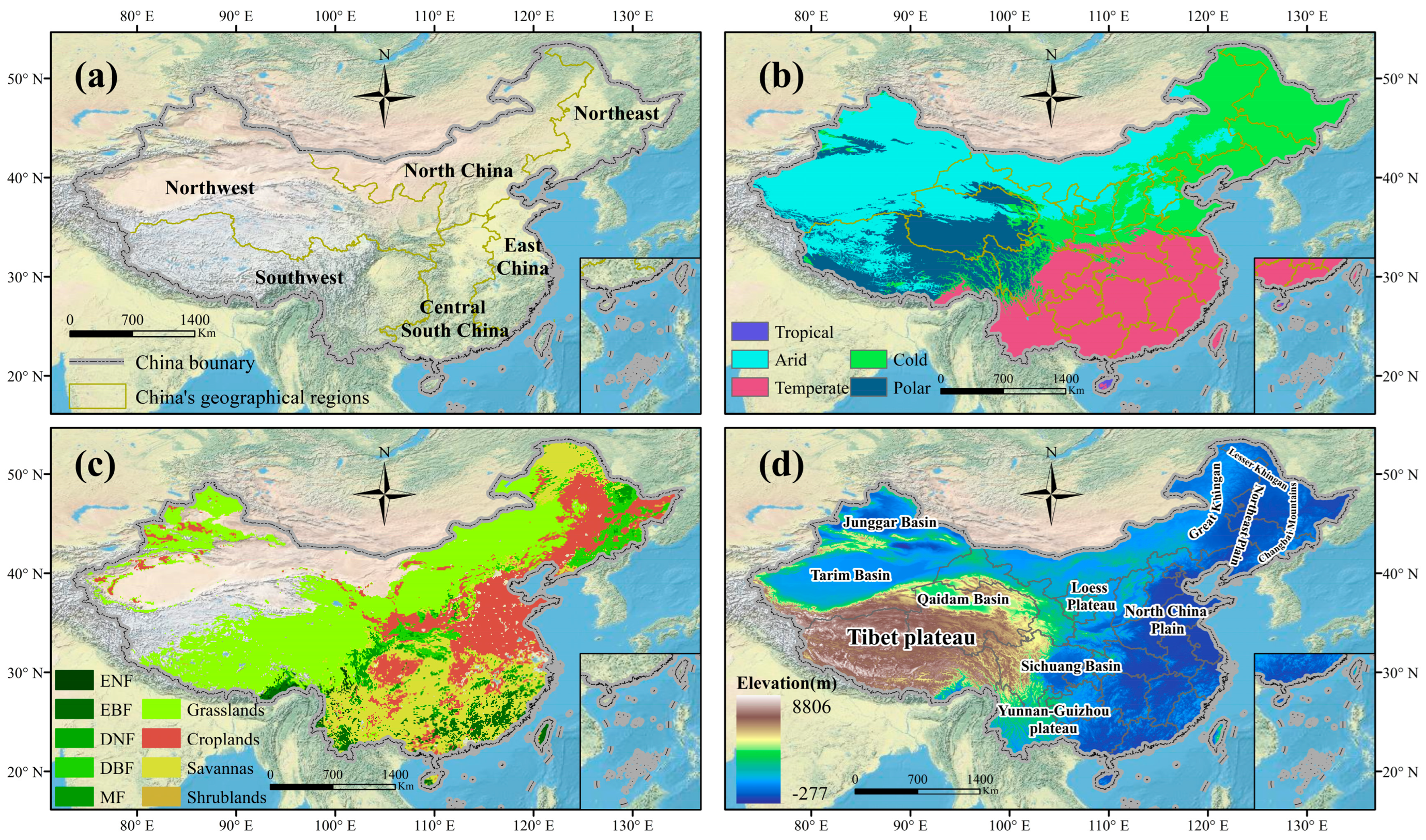
Figure 1. Overview of the study area, showing (a) the six geographical divisions of China, (b) the Köppen climate classification [33], (c) the vegetation type distribution, and (d) the elevation map. The basemap is provided by the US National Park Service (https://services.arcgisonline.com/ (accessed on 5 January 2026)).
Remotesensing 18 00275 g001
Figure 2. Sen’s slope (g C m−2 d−1) of GPP in China during 2001–2020 and the Mann–Kendall test for (a) annual, (b) growing season (May to September), (c) spring, (d) summer, (e) autumn, and (f) winter. Colors represent the Sen’s slope, and asterisks indicate regions with statistically significant trends (p < 0.05) at the 0.1° resolution.
Remotesensing 18 00275 g002
Figure 3. Time series and trends of regional mean GPP (g C m−2 d−1) across six regions in China during 2001–2020: (a) Northeast China, (b) North China, (c) East China, (d) Northwest China, (e) Southwest China, and (f) Central South China. Red dashed lines represent linear trends estimated using the Mann–Kendall test and Sen’s slope (g C m−2 d−1 yr−1). Asterisks indicate statistically significant trends (*** p < 0.001).
Remotesensing 18 00275 g003
Figure 4. Significant GPP trends (p < 0.05, 2001–2020) under different vegetation types in China, indicated by Sen’s slope (↑ increase, ↓ decrease) and the Mann–Kendall test for (a) annual, (b) growing season (May to September), (c) spring, (d) summer, (e) autumn, and (f) winter.
Remotesensing 18 00275 g004
Figure 5. Spatial distribution of stable vegetation types and temporal trends of regional mean GPP (g C m−2 d−2) for different vegetation categories in China during 2001–2020: (a) ENF, (b) EBF, (c) DNF, (d) DBF, (e) MF, (f) Grasslands, (g) Croplands, (h) Savannas, and (i) Shrublands. Red dashed lines represent linear trends estimated using the Mann–Kendall test and Sen’s slope (g C m−2 d−1 yr−1). Asterisks indicate statistically significant trends (** p < 0.01, *** p < 0.001), while “ns” denotes non-significant trends.
Remotesensing 18 00275 g005
Figure 6. Histogram of SHAP contributions (%) (ratio of each factor’s SHAP to the sum of all absolute SHAP) of individual impact factors across different vegetation types ((a) ENF, (b) EBF, (c) DNF, (d) DBF, (e) MF, (f) Grasslands, (g) Croplands, (h) Savannas, (i) Shrublands, and (j) ALL), with inset pie charts showing the normalized percentage contributions of the four variable categories (i.e., climate, vegetation, topography, and human activity).
Remotesensing 18 00275 g006
Figure 7. Violin plots of SHAP percentages (%, ratio of each factor’s SHAP to the mean predicted GPP) for individual impact factors across different vegetation types: (a) ENF, (b) EBF, (c) DNF, (d) DBF, (e) MF, (f) Grasslands, (g) Croplands, (h) Savannas, (i) Shrublands, and (j) ALL.
Remotesensing 18 00275 g007
Figure 8. Heatmap of SHAP interaction contribution (%) among multiple impact factors across different vegetation types ((a) ENF, (b) EBF, (c) DNF, (d) DBF, (e) MF, (f) Grasslands, (g) Croplands, (h) Savannas, (i) Shrublands, and (j) ALL), showing the ratio of each factor’s SHAP to the sum of all absolute SHAP. Note: Variables are abbreviated as follows: climate (C1–C6: PRECIP, PSFC, RH, SWDOWN, T2D, VPD), vegetation (V1–V2: LAI, LSWI), topography (T1–T3: Elevation, Slope, Aspect), and human activity (H1–H4: HII, PD, LSI, AI). Numeric labels are omitted for values < 0.2.
Remotesensing 18 00275 g008
Figure 9. SHAP Interaction heatmap of vegetation and climatic variables across all ecosystems.
Remotesensing 18 00275 g009
Figure 10. SHAP Interaction heatmap of vegetation and human variables activities across all ecosystems.
Remotesensing 18 00275 g010
Disclaimer/Publisher’s Note: The statements, opinions and data contained in all publications are solely those of the individual author(s) and contributor(s) and not of MDPI and/or the editor(s). MDPI and/or the editor(s) disclaim responsibility for any injury to people or property resulting from any ideas, methods, instructions or products referred to in the content.