Article

A New Sea Ice Concentration (SIC) Retrieval Algorithm for Spaceborne L-Band Brightness Temperature (TB) Data

1
Department of Atmospheric and Oceanic Sciences & Institute of Atmospheric Sciences, Fudan University, Shanghai 200438, China
2
Zhuhai Fudan Innovation Research Institute, Zhuhai 519000, China
3
Shanghai Key Laboratory of Ocean-Land-Atmosphere Boundary Dynamics and Climate Change, Shanghai 200438, China
4
Key Laboratory of Polar Atmosphere-Ocean-Ice System for Weather and Climate, Ministry of Education, Fudan University, Shanghai 200438, China
5
Department of Water Resources, Faculty of Geo-Information Science and Earth Observation (ITC), University of Twente, 7500 AE Enschede, The Netherlands
6
School of Atmospheric Sciences, Chengdu University of Information Technology, Chengdu 610225, China
7
The Plateau Atmosphere and Environment Key Laboratory of Sichuan Province, Chengdu University of Information Technology, Chengdu 610225, China
*
Author to whom correspondence should be addressed.
Remote Sens. 2026, 18(2), 265; https://doi.org/10.3390/rs18020265
Submission received: 14 December 2025 / Revised: 4 January 2026 / Accepted: 12 January 2026 / Published: 14 January 2026

Highlights

What are the main findings?
  • A novel L-band sea ice concentration retrieval algorithm has been developed, which systematically quantifies and constrains four key uncertainties—particularly the Diurnal Amplitude Variation (DAV) signal associated with sea ice freeze–thaw cycles.
  • DAV exhibits the most pronounced effect on the precision of the sea ice concentration retrieval algorithm; constraining all four key uncertainties together achieves a further reduction in RMSE to 7.42%.
What are the implications of the main findings?
  • The novel L-band sea ice concentration retrieval algorithm consistently demonstrates high agreement with SSM/I, ship-based SIC data, and SAR SIC, supporting its reliability under various validation scenarios.
  • Integrating the DAV signal into future retrieval models can enhance the understanding of sea ice freeze–thaw processes and improve ice-atmosphere interaction studies in climate modeling and data assimilation.

Abstract

Sea ice concentration (SIC) is crucial to the global climate. In this study, a new single-channel SIC retrieval algorithm utilizing spaceborne L-band brightness temperature (TB) measurements is developed based on a microwave radiative transfer model. Additionally, its four uncertainties are quantified and constrained: (1) variations in seawater reference TB under warm water conditions, (2) variations in sea ice reference TB under extremely low-temperature conditions, (3) the freeze–thaw dynamics of sea ice captured by Diurnal Amplitude Variation (DAV) signals, and (4) Land mask imperfections. It is found that DAV has the most pronounced effect: eliminating its influence reduces RMSE from 10.51% to 8.43%, increases R from 0.92 to 0.94, and minimizes Bias from -0.68 to 0.13. Suppressing all four uncertainties lowers RMSE to 7.42% (a 3% improvement). Furthermore, the algorithm exhibits robust agreement with the seasonal variability of SSM/I SIC, with R mostly exceeding 0.9, RMSE mostly below 10%, and Biases mostly within 5% throughout the year. Compared to ship-based and SAR SIC data, the new L-band algorithm’s Bias and RMSE are only 2% and 2% (ship-based)/2% and 1% (SAR) higher, respectively, than those of the SSM/I product. Future algorithms can integrate the DAV signal more effectively to better understand sea ice freeze–thaw processes and ice-atmosphere interactions.

1. Introduction

Sea ice is a critical component of the global climate system. Its high albedo reflects a substantial portion of incoming solar radiation, playing a key role in regulating the Earth’s energy balance [1]. Sea ice concentration (SIC), defined as the percentage of a given ocean area covered by sea ice [2], is a fundamental geophysical variable. Declines in SIC reduce surface albedo, enhancing solar absorption by the ocean and triggering a potent ice-albedo feedback that amplifies Arctic warming [3,4]. Furthermore, changes in SIC modulate heat and moisture fluxes between the ocean and atmosphere, influencing regional and global atmospheric circulation patterns [5]. Therefore, obtaining accurate, long-term SIC records is essential for climate research and prediction.
Since the 1970s, remote sensing, particularly passive microwave remote sensing, has been utilized for SIC monitoring. Space-based passive microwave remote sensing instruments can measure microwave radiation emitted by Earth’s surface. It operates continuously, day and night, and penetrates cloud cover [6,7]. Several SIC algorithms have been developed for sensors, including the Scanning Multi-Frequency Microwave Radiometer (SMMR) [8], the Advanced Microwave Scanning Radiometer 2 (AMSR-2), and the Advanced Microwave Scanning Radiometer for EOS (AMSR-E) sensor data [9]. For example, NASA Team [10] and Bootstrap [11] utilized brightness temperature (TB) data at 19 GHz and 37 GHz to retrieve SIC. Pedersen [12] obtained SIC by using 6 GHz horizontally polarized TB data from the Electrically Scanning Microwave Radiometer (EMSR) sensor. NASA Team 2 [13] and the Turbulence Interaction Study Sea Ice (TISI) method [14] used channels above 85 GHz to enhance the spatial resolution of SIC products. Enhancements, including the dynamic selection of reference TB [15,16], the correction of atmospheric effects [17], the optimization of radiative transfer models [18], and the continuous development of operational products such as the EUMETSAT Ocean and Sea Ice Satellite Application Facility (OSI SAF) SIC algorithm [19], have improved the stability of the SIC product. Recently, deep learning approaches have been explored for SIC retrieval [20,21,22], but challenges in generalization and physical interpretability remain, leaving physical passive microwave SIC algorithms as the operational mainstay.
Despite the proliferation of passive microwave SIC algorithms, their accuracy and robustness are highly condition-dependent, exhibiting significant sensitivity to environmental factors. Comparative analyses reveal substantial inter-algorithm discrepancies, with reported differences often reaching ±10%, attributable to variations in frequency selection, polarization, and tie-point definitions [23,24]. When validated against in situ or high-resolution data, a limitation emerges: root-mean-square errors (RMSE) typically range from 10% to 20%, with a pronounced degradation in accuracy during summer melt seasons and within the dynamic marginal ice zone [25,26,27]. This limitation gap highlights a critical challenge: existing algorithms struggle to accurately capture the complex thermodynamic and physical states of sea ice during periods of transition and melt, when surface conditions are most variable. These retrieval uncertainties directly limit the utility of SIC products in downstream applications, such as numerical weather prediction and climate reanalysis. For example, while systems like the ECMWF’s ocean reanalysis (ORAS5) [28] assimilate operational passive microwave SIC data [29], the inherent errors and spatial representativeness issues in current products constrain their effectiveness [30]. Furthermore, key processes, such as melt ponds, remain unrepresented in forecast models [31]. Consequently, there is a recognized need to improve retrieval accuracy and to integrate more robust, physically constrained observations into these systems [32].
The L-band (1.4 GHz), employed by the Soil Moisture and Ocean Salinity (SMOS) and Soil Moisture Active Passive (SMAP) missions, offers a complementary observational perspective. Its longer wavelength provides deeper penetration with minimal atmospheric interference, yielding a TB signal more directly tied to surface properties and showing higher sensitivity to SIC variations [33]. Although its spatial resolution is coarser (~40 km), it is suitable for climate-scale studies and has proven valuable for sea ice thickness estimation [32]. Initial studies have demonstrated the feasibility of L-band SIC retrieval using multi-angle [34] or polarization-difference approaches [33].
Although the L-band is more sensitive to SIC than other frequencies, Kilic et al. [35] revealed that emissivity variations of sea ice and seawater in this spectral band demonstrate considerable amplitude and fluctuation. Therefore, exploiting the full potential of L-band for operational SIC retrieval requires confronting its specific sources of uncertainty, which are distinct from those at higher frequencies. The accuracy of single-channel algorithms hinges on stable reference TB for pure water (SIC = 0%) and pure ice (SIC = 100%). First is the uncertainty of the reference TB for seawater. In regions with relatively high sea surface temperatures, warm water may easily be misclassified as sea ice, causing fluctuations in the seawater reference TB [19,36]. Second is the uncertainty of the reference TB for sea ice. Under extremely low temperatures, variations in physical properties such as age and structure may lead to fluctuations in the sea ice reference TB [37,38]. Third is the sea ice freeze–thaw process. Traditional SIC algorithms, which assume constant emissivity, are unable to account for this process. However, the Diurnal Amplitude Variation (DAV) signal, which captures the differences in TB between ascending and descending orbits, reflects these dynamic changes. Studies have shown that the DAV signal is susceptible to soil freeze–thaw cycles and snowmelt processes [39,40,41,42]. Due to the significant contrast in dielectric constants between sea ice and liquid water [43], this sensitivity also exists in sea ice retrieval. During sea ice melting and refreezing, ice and water may coexist within the footprint of a given instrument, resulting in emissivity variations that are reflected in the DAV signal. Finally, the limited spatial resolution of low-frequency passive microwave instruments may be compromised by radiation from nearby land surfaces, leading to misclassification.
To address these challenges, this study develops a novel L-band SIC retrieval framework based on multi-physical constraint collaborative optimization. Beyond conventional constraints like sea surface temperature (SST), ice surface temperature (IST), and land masking, this method integrates the L-band DAV as a dynamic, process-oriented constraint. The inclusion of DAV not only directly addresses the freeze–thaw uncertainty, a significant weakness of existing algorithms, but also adds a valuable “surface state stability” layer to the SIC product, thereby enhancing its interpretability for studies of the marginal ice zone and melt processes. Section 2 describes the datasets, and Section 3 details the methodology, including the base algorithm and the multi-constraint optimization process. Section 4 presents the results of uncertainty quantification, algorithm optimization, and validation. Section 5 discusses the broader implications and advantages of the approach, and Section 6 provides the conclusion.

2. Data

This study utilizes multiple satellite, reanalysis, and in situ datasets to develop and validate a L-band sea ice concentration (SIC) retrieval algorithm for the period from 1 July 2020, to 30 June 2021. For clarity, the key datasets are summarized in Table 1, organized by their primary function within the study. SMAP L-band TB observations serve as the fundamental input for the retrieval. ERA5 reanalysis data are used to define physical constraints and endmembers. Daily SIC from SSM/I-SSMIS provides a primary reference for algorithm optimization and evaluation, while independent ship-based observations and high-resolution SAR SIC data are used for robust, multi-source validation.

2.1. Core Input: SMAP L-Band Brightness Temperature

The SMAP satellite provides stable L-band (1.4 GHz) observations with a fixed 40° incidence angle and advanced radio-frequency interference mitigation [44]. The TB at the L-band is more sensitive to SIC under horizontal than vertical polarization [35]. Therefore, this study uses the horizontally polarized TB from the SMAP L3 Radiometer Daily 36 km EASE-Grid Freeze/Thaw State product (SPL3FTP, Version 3) [45]. The product’s consistent observation geometry and real-aperture design ensure that ascending and descending TB differences directly reflect diurnal surface variations, making it ideal for analyzing the freeze–thaw-related Diurnal Amplitude Variation (DAV). Missing passes are filled via interpolation in official products [46]. Ascending and descending pass brightness temperatures are averaged to produce a daily value for each grid cell over the Arctic study region (north of 30.98°N). Figure 1 presents an example of daily averaged gridded TB over the Arctic on January 1, 2021, illustrating the spatial coverage and typical brightness temperature range captured by SMAP for this study. The data can be accessed at the following website: https://nsidc.org/data/spl3ftp/versions/3 (accessed on 10 November 2023) [45].

2.2. Constraint and Endmember Definition: ERA5 Reanalysis

ERA5 reanalysis data from ECMWF provide a physically consistent, global estimate of key surface variables [47] based on all available information. In this study, they are used for three specific purposes: (1) SIC fields are used to identify large, stable regions for defining pure ice and pure water radiometric endmembers, following established methodologies [47,48]; (2) Sea surface temperature (SST) and (3) the temperature of the top 0–7 cm ice layer are used to quantify and constrain the impact of warm water and extremely low temperature condition of ice on TB, which are key sources of retrieval uncertainty. Hourly ERA5 data (SIC, SST, ice temperature) are averaged to daily means, and spatially resampled to match the 36 km SMAP grid. Hourly ERA5 data can be accessed through the ECMWF’s official website (https://cds.climate.copernicus.eu/cdsapp#!/dataset/reanalysis-era5-single-levels?tab=overview) (accessed on 15 June 2024) [49].

2.3. Primary Reference: SSM/I-SSMIS Sea Ice Concentration

Daily SIC data from the “Sea Ice Concentrations from Nimbus-7 SMMR and DMSP SSM/I-SSMIS” product (Version 2, NASA Team algorithm) [50] serve as the primary reference dataset. The generation of this SIC dataset utilizes the NASA Team algorithm, which uses the differences in TB under various polarizations and frequency bands to effectively distinguish between the characteristics of sea ice and seawater [10]. This long-term, widely used climate data record provides a standard benchmark in climate studies [51,52], as well as for SIC algorithm comparisons and validation [53,54]. In this study, it is used extensively during the algorithm development phase for threshold evaluation, optimization, and comparative performance assessment against the new L-band retrievals. SSM/I SIC data can be obtained from the NSIDC website (https://nsidc.org/data/nsidc-0051/versions/2) (accessed on 15 June 2024) [50].

2.4. Independent Validation Data

To ensure robust evaluation, the algorithm is validated against two independent datasets with different spatial characteristics.
(1)
Ship-Based Observations: Visual SIC estimates from the ICEWatch/ASSIST program (https://cryo.met.no/en/icewatch) (accessed on 25 February 2025) [55] provide in situ point measurements within an approximate 1 km radius of the vessel. Observers use integer values from 0 to 10 to describe the sea ice conditions, corresponding to SIC ranging from open water (0%) to consolidated ice (100%). Following the method of Beitsch et al. [56], each daily ship record is matched to the nearest satellite grid cell for comparison, offering a ground-truth perspective.
(2)
High-Resolution SAR SIC: This study has been conducted using E.U. Copernicus Marine Service Information, specifically the SAR sea ice concentration (SIC) product; https://doi.org/10.48670/mds-00344 (accessed on 24 November 2025) [57]. The 1 km resolution Arctic Ocean High-Resolution Sea Ice L4 product, which blends Sentinel-1 and RCM SAR imagery and GCOM-W AMSR2 microwave radiometer data using deep learning methods, provides a spatially detailed reference. For a fair comparison at the SMAP scale, all 1 km pixels within a given SMAP grid cell are averaged to produce a single, co-located reference SIC value for validation against both the new L-band and resampled SSM/I SIC.

3. Methods

3.1. Single-Channel Algorithm

The microwave radiation transfer model is the forward model for retrieving surface parameters. It describes the propagation process of microwave signals between the atmosphere and the surface [12]. The model also quantifies the various contributions that affect the microwave brightness temperature received by satellites.
T B = T s e τ + T 1 + 1 ε T 2 e τ + 1 ε T s p e 2 τ
where ε represents the emissivity. τ denotes the atmospheric optical thickness. T s refers to the surface radiation temperature. T 1 indicates the upward radiation of the atmosphere. T 2 represents the downward radiation TB of the atmosphere. T s p signifies the cosmic background radiation TB Due to the particular polar atmospheric conditions, the last three terms can be neglected [33]. In polar regions, humidity is low, and there are almost no liquid water droplets present. Typically, only low clouds exist, with an insignificant liquid water content. As a result, the optical thickness τ is minimal and can be neglected. The assumption e τ = 1 τ can be used. Then, the microwave radiation transfer model for polar regions is simplified to:
T B = T s = ε t s
The TB that the radiometer receives is approximately equal to the radiation brightness temperature of the Earth’s surface. It is influenced by two main factors: the surface emissivity ε and the physical temperature t s . Based on the microwave radiation transfer model above, the differences in microwave radiation properties between sea ice and seawater can be examined. The SMAP satellite’s field of view is assumed only to include seawater and sea ice. Consequently, the TB received by the satellite can be expressed as:
T B = 1 C ε w t w + C ε I t I
C = T B ε w t w ε I t I ε w t w = T B T B w a t e r T B i c e T B w a t e r
Here, C represents the proportion of ice within a satellite’s field of view, which is defined as SIC. ε I and ε w represent the emissivity of sea ice and seawater, respectively. t I and t w represent the physical temperature of sea ice and seawater, respectively. The brightness temperature observed by the satellite radiometer is denoted as TB. The reference TB corresponding to sea ice and seawater is represented as T B i c e and T B w a t e r , respectively. Therefore, if T B i c e and T B w a t e r are known, along with the TB observed by the radiometer, the C can be derived, which indicates SIC. C and TB can be expressed using a linear equation, as shown below.
C = a × T B + b
a = 1 T B i c e T B w a t e r ; b = T B w a t e r T B i c e T B w a t e r

3.2. Parameter Calibration and Uncertainty Minimization for SIC Retrieval

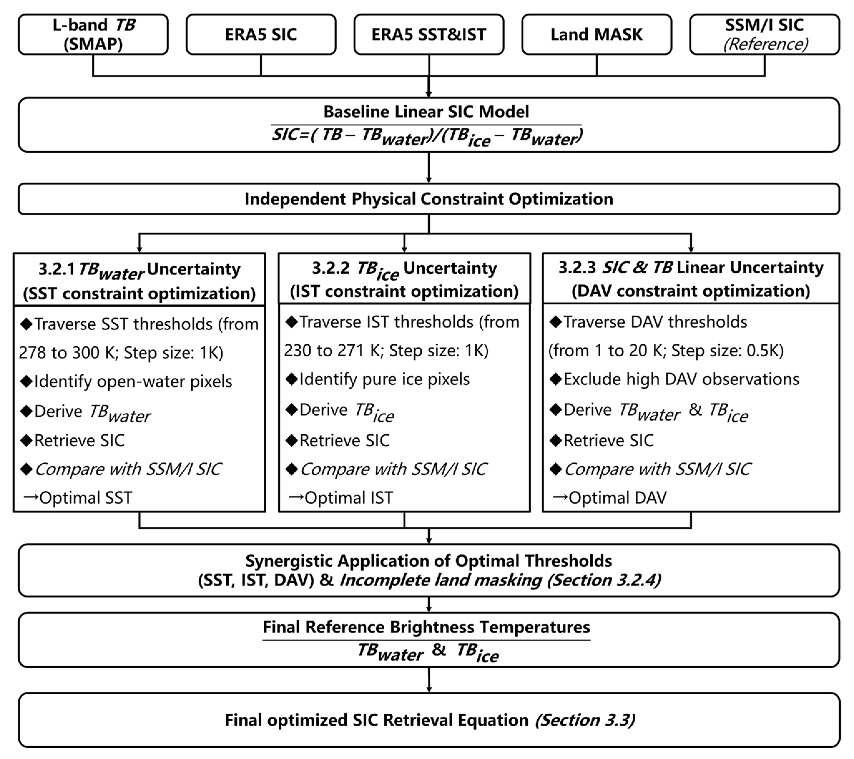
To reduce uncertainties in L-band SIC retrieval, a synergistic optimization framework is proposed based on Equation (4). It explicitly incorporates four primary sources of uncertainty. Specifically, SST governs the emissivity variability of open water, IST controls the emissivity variability of sea ice. And DAV characterizes the dielectric instability induced by freeze-thaw cycles. This instability introduces nonlinearity into the relationship between SIC and TB. Figure 2 presents a detailed flowchart of the proposed framework, illustrating how these physical constraints are implemented and combined within the retrieval process. Starting from a baseline linear SIC formulation, the uncertainties associated with SST, IST, and DAV are addressed through three independent optimization procedures. For each constraint, a range of physically meaningful thresholds is traversed to identify the reference TB of open-water or pure-ice, derive corresponding TBwater and TBice, and evaluate the resulting SIC retrieval against an independent SSM/I SIC product. The optimization procedures for SST, IST, and DAV are described in Section 3.2.1, Section 3.2.2 and Section 3.2.3, respectively. The land mask is not subject to threshold optimization and is applied as a fixed physical constraint, as described in Section 3.2.4. After these independent optimization constraints, all four uncertainty components are used simultaneously to construct a physically consistent set of TBwater and TBice. These optimized reference brightness temperatures form the basis of the final SIC retrieval equation, which is presented in Section 3.3.

3.2.1. Seawater Reference TB (TBwater) and Uncertainty Optimization

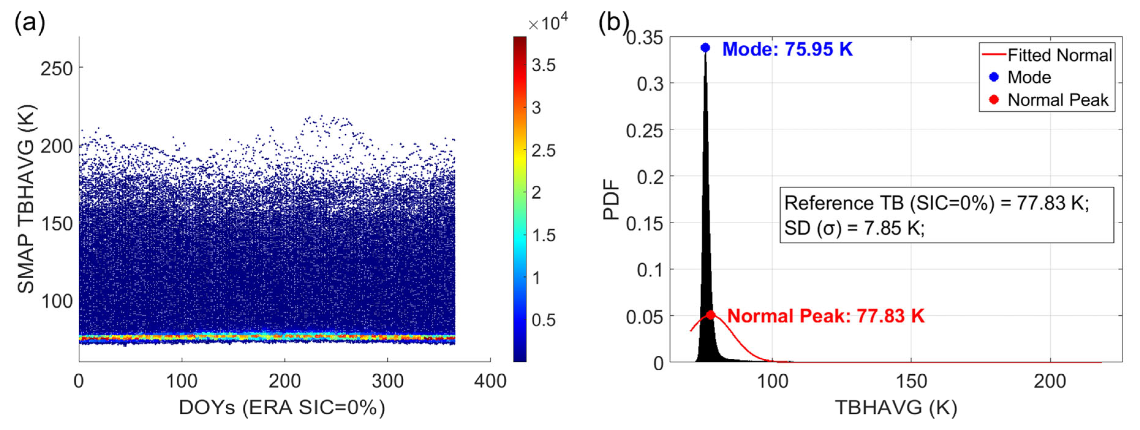
When performing SIC retrieval, it is necessary to determine TBwater. TBwater refers to the TB that reflects typical seawater (open water) conditions [23] and provides the lower boundary condition for Equation (6). To obtain TBwater, the “seawater” type is defined as regions that maintain ERA5 SIC = 0% throughout the year. In addition, for cases where ERA5 SIC = 0% but SST is below 278 K, these regions are excluded. This value, set notably above the freezing point of seawater, aims to rigorously exclude the radiative influence of sub-pixel sea ice, thereby ensuring the selection of pure open water for defining a stable brightness temperature signature. The selection of this threshold reference is a well-established practice in passive microwave sea ice retrieval [47,48,58]. Following the concept of single-channel algorithms [12], the reference TB for these “seawater” regions is calculated as the mean TB within the area. Averaging effectively reduces random fluctuations caused by environmental noise. Figure 3a illustrates the spatial distribution of typical seawater regions, where the temperature fluctuates between 70 and 200 K, with most values concentrated in the 70–80 K range. Figure 3b presents the probability density distribution of the daily mean TB for these regions. Statistical results indicate that the mean TB for typical open water is 77.83 K, with a standard deviation of 7.85 K. Therefore, this study adopts 77.83 K as the reference TB for seawater.
However, in practical applications, the uncertainty of TBwater must be considered. The primary sources of this uncertainty include observational noise and short-term variations in seawater physical properties, such as temperature [19,36]. These uncertainties can cause seawater TB to resemble those of sea ice under certain conditions, leading to errors in SIC retrieval. To reduce the uncertainty of the seawater reference TB, this study introduces ERA5 sea surface temperature (SST) as a constraint. Using this procedure, a new seawater reference TB can be obtained. Additionally, these abnormal SST samples are excluded when evaluating retrieval accuracy based on SSM/I SIC.
To determine the SST constraint threshold, the initial range is set from 278 K to 310 K. When ERA5 SST exceeds a certain threshold, the area is classified as open water, and SIC is set to 0%. The threshold is adjusted stepwise with an increment of 1 K. Each new SST threshold generates a new reference TB. The corresponding TBwater is then used for SIC retrieval. SSM/I products are chosen as the optimization criterion because they have been validated over many years and are considered a reliable benchmark for monitoring polar sea ice. The results are shown in Figure 4. As the SST constraint threshold increases, Bias decreases in the 278–285 K range. However, RMSE exhibits a logarithmic increase, with a growth rate larger than the decrease in Bias and the increase in R. Considering all three metrics, 278 K is selected as the SST constraint threshold to obtain the new seawater reference TB.

3.2.2. Sea Ice Reference TB (TBice) and Uncertainty Optimization

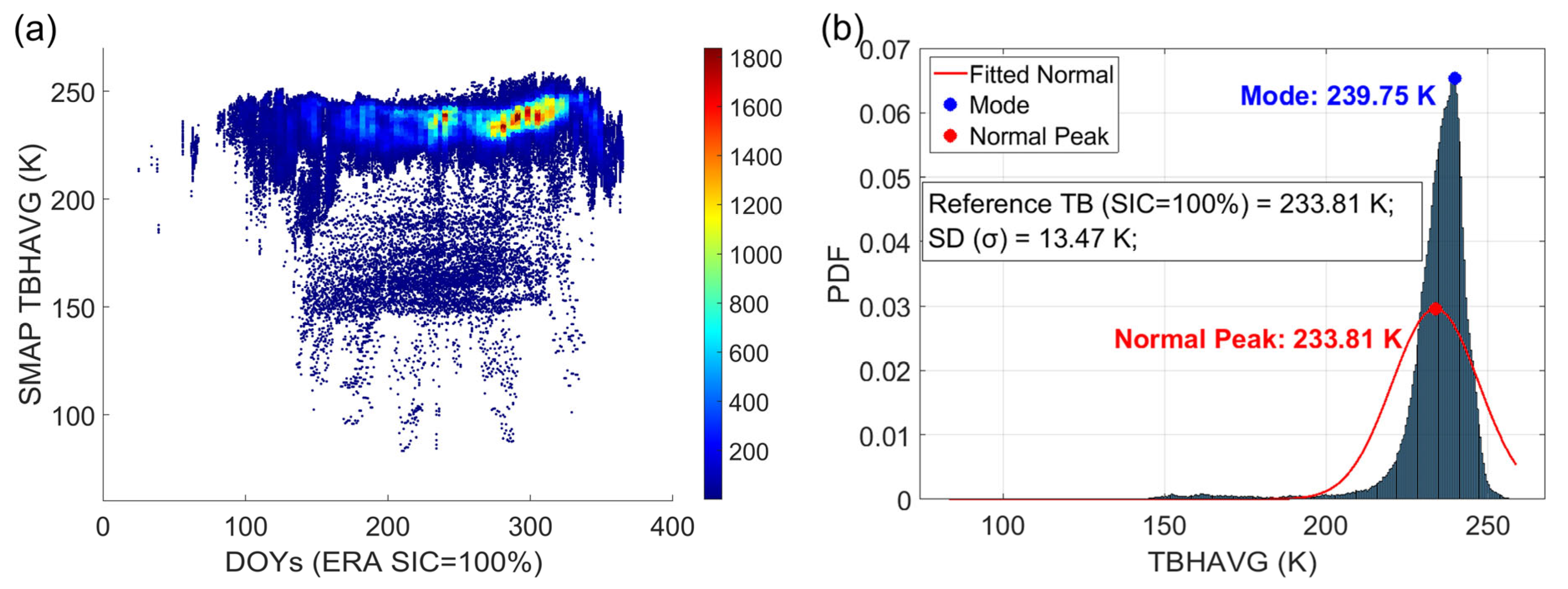
In SIC retrieval, TBice corresponds to fully ice-covered conditions (SIC = 100%), which provides the upper boundary condition for Equation (6). To obtain TBice, the “fully ice-covered” type is defined as regions that maintain ERA5 SIC = 100%. The mean TB is then extracted from these regions. Figure 5a shows the TB distribution in a typical 100% ice-covered area. The distribution ranges from 150 K to 250 K. Most values are concentrated around 230 K. Figure 5b presents the probability density distribution of the daily mean TB. Statistical results indicate that the mean TB for fully ice-covered conditions (SIC = 100%) is 233.81 K, with a standard deviation of 13.47 K. Therefore, 233.81 K is selected as the reference TB for typical fully ice-covered regions.
However, TBice still contains multiple sources of uncertainty. The primary sources include variations in sea ice type, age, and structure. For example, the emissivity of sea ice is controlled by its internal components, such as ice, brine, and air bubbles [37,38]. These mixed components alter the radiative properties of sea ice. To reduce these uncertainties, this study introduces a new constraint threshold based on IST from ERA5. IST represents the ice temperature of the upper 0–7 cm ice layer. Candidate IST thresholds are first set from 230 K to 271 K with a step of 1 K. Ice samples with IST lower than each candidate threshold are excluded. Each IST threshold condition generates a different TBice. Each TBice is then substituted into the single-channel algorithm to calculate SIC. The SIC results are compared with independent SSM/I products. Figure 6a shows Bias, Figure 6b shows RMSE, and Figure 6c shows R. As the IST threshold increases, Bias becomes stable in the range of 230–260 K. After this range, Bias shifts from negative to positive. RMSE reaches its minimum at 242 K. The reduction in RMSE at 242 K is larger than the improvement in R. Based on the overall comparison, this study selects 242 K as the optimal constraint IST threshold for a new TBice. This likely excludes mainly multiyear ice, which has smaller TB and IST than first-year ice.

3.2.3. Establishing and Optimizing the Linear Relationship Between SIC and TB

In addition to the uncertainty in determining the reference TB of seawater (SIC = 0%) and sea ice (SIC = 100%), the retrieval of SIC from L-band TB also relies on a linear relationship. This linear relationship connects SIC to TB In the first step, the uncertainties of seawater and sea ice are ignored. Ignoring these uncertainties means that no constraint conditions are applied. Under these conditions, the results from Figure 3 and Figure 5 serve as the reference TB for seawater (SIC = 0%) and sea ice (SIC = 100%). These reference brightness temperatures are then substituted into Equations (5) and (6). Substitution of two reference brightness temperatures establishes the SIC retrieval equation. This process produces Equation (7).
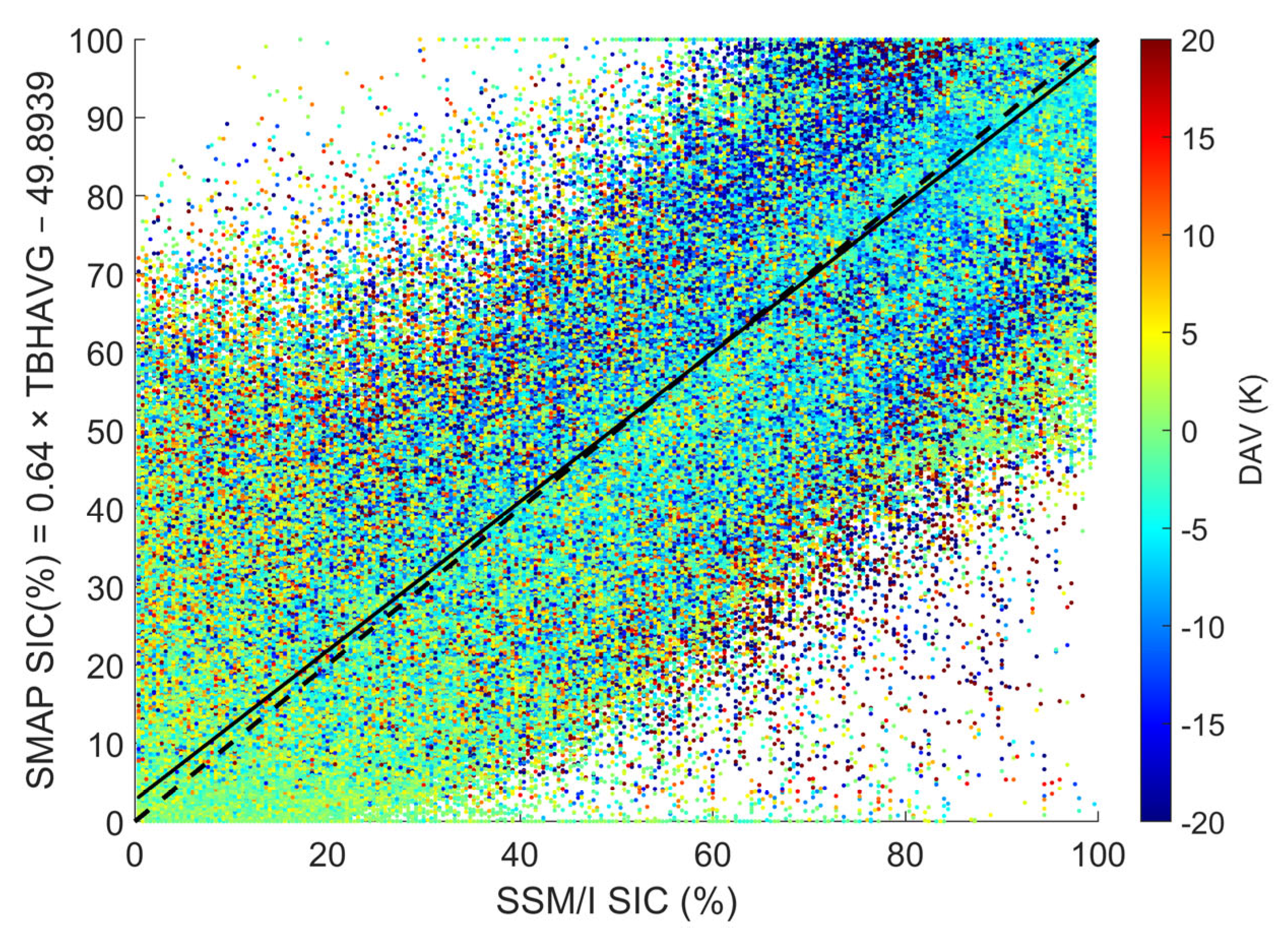
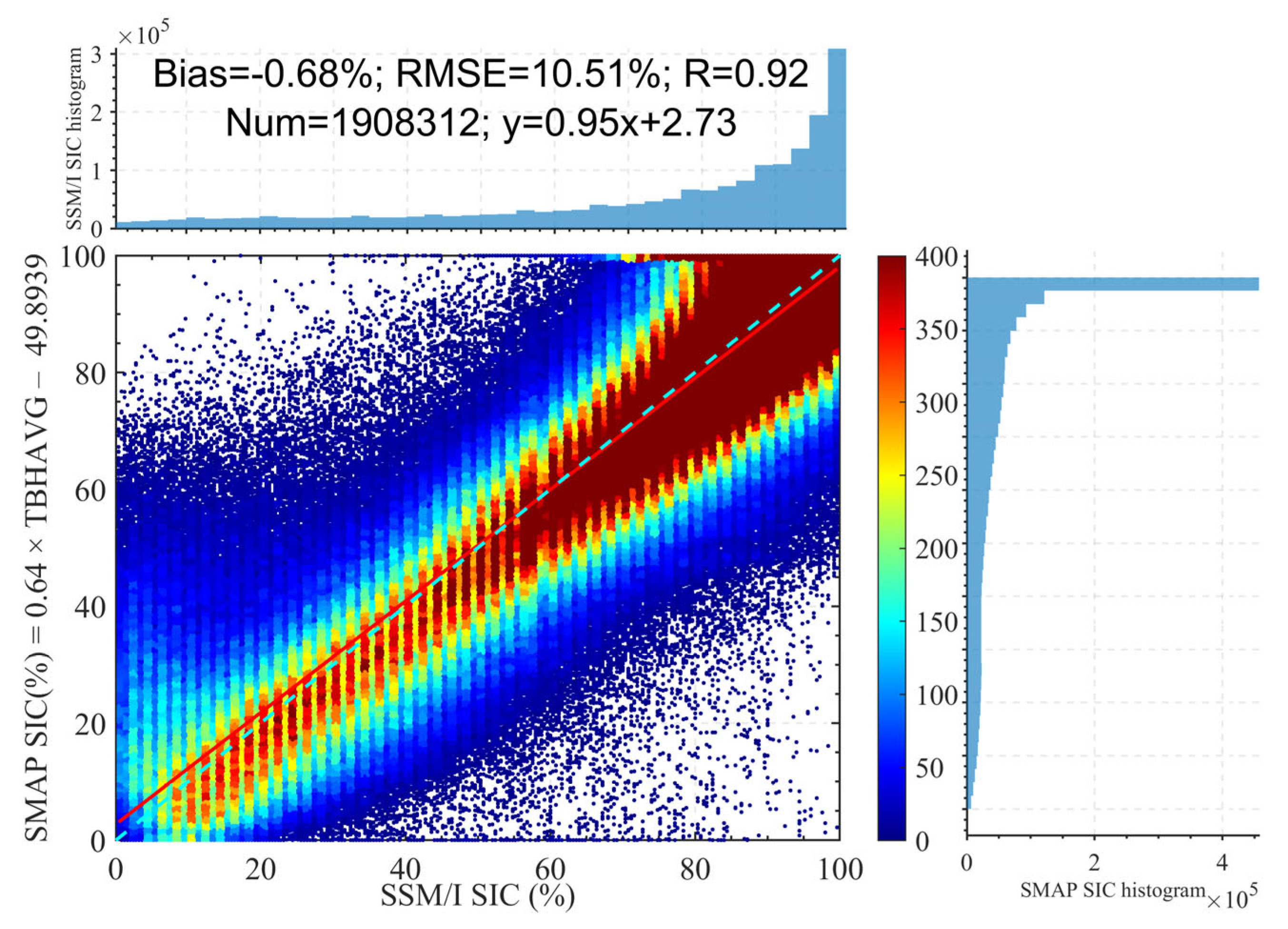
S I C = 0.64 × T B 49.8939
However, this linear relationship also contains multiple sources of uncertainty. Figure 7 shows the comparison between the SIC retrieved from Equation (7) and the SSM/I products. In Figure 7, the scatter points are color-coded by DAV. The results show that points with larger DAV often deviate from the linear trend between SSM/I SIC and L-band SIC, which TBwater and TBice derive. This finding suggests that the magnitude of DAV is closely related to the linear correlation in the SIC regression. In regions with large DAV, sea ice may experience melting and refreezing. Melting and refreezing interfere with the observed TB through physical processes. Such interference causes deviations from the ideal linear relationship and introduces retrieval errors in SIC. Specifically, according to Equations (8) and (9), the TB observed by the radiometer mainly depends on the surface emissivity (ε) and the physical temperature (ts). When no melting or freezing occurs in water or ice, the variation in emissivity is usually small. In this situation, DAV should be smaller than the change in physical temperature. However, during freeze–thaw cycles, emissivity changes largely, which induces fluctuations in TB. Therefore, if DAV exceeds this expected range, the observation is likely influenced by the freeze–thaw process of sea ice.
Δ t s = t s / 6   p . m . t s / 6   a . m .
D A V = T B 6   p . m . T B 6   a . m . < ε Δ t s
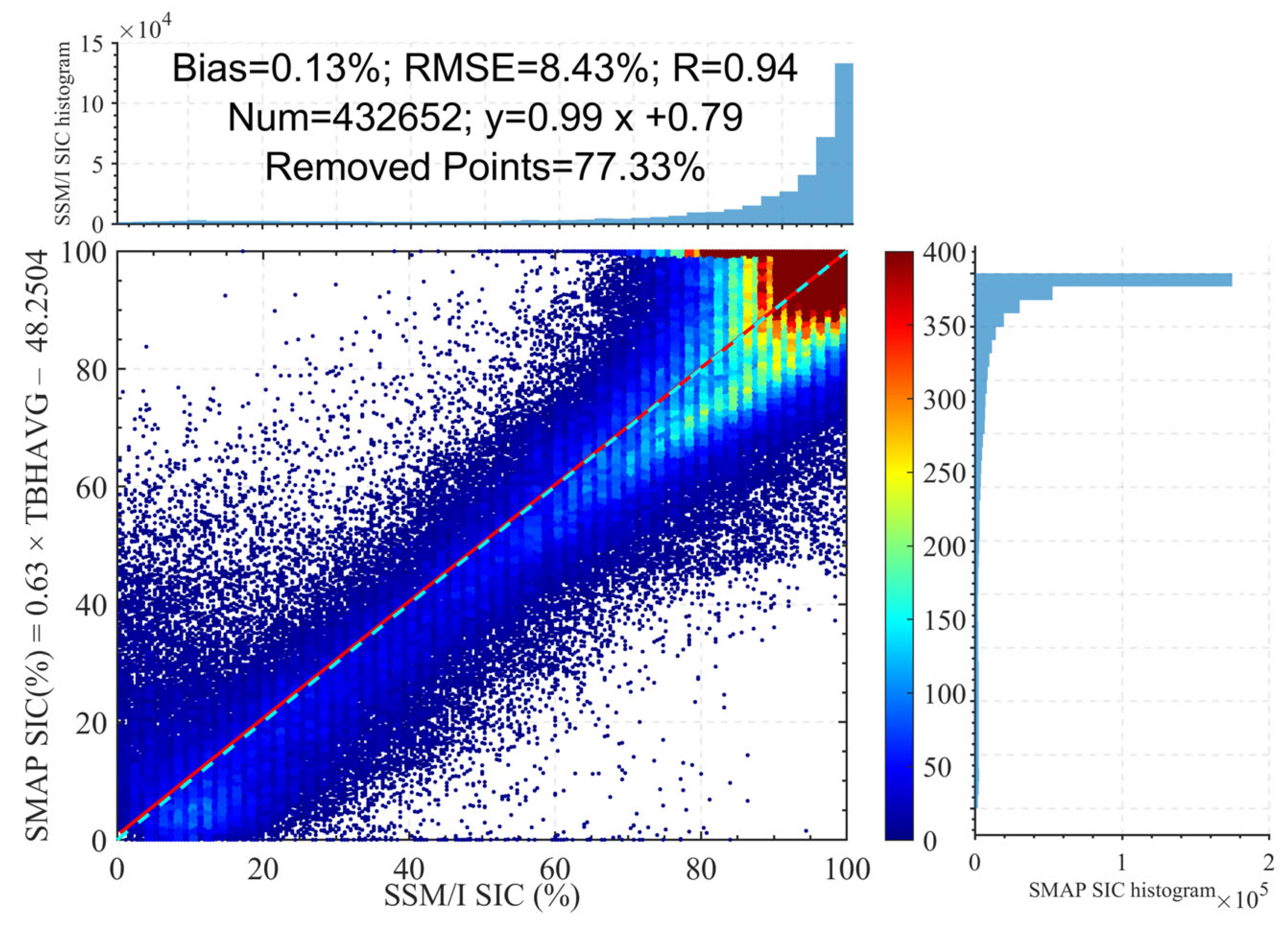
To quantify the impact of sea ice freeze–thaw processes on SIC retrieval, this study introduces DAV as an indicator. DAV reflects TB variations caused by the freeze–thaw processes of sea ice. DAV is usually derived from the difference between ascending and descending satellite TB. Previous studies [39,40,41,42] have shown that DAV effectively characterizes the freeze–thaw cycles of soil or snow. The mechanism originates from the emissivity differences between liquid water and snow, as well as the dielectric constant differences between frozen and unfrozen soil. For sea ice, the coexistence of ice and water also modifies emissivity [43]. This modification changes the observed TB. To reduce the uncertainty caused by freeze–thaw processes represented by DAV signals, this study applies a constraint threshold to DAV. The threshold range is set from 1 K to 20 K with a step size of 0.5 K. At each step, TB samples with abnormally high DAV are excluded. Each new DAV threshold produces new TBwater and TBice. These new reference brightness temperatures generate a new SIC retrieval equation. Figure 8a presents Bias, Figure 8b presents RMSE, and Figure 8c presents R. The results show that as the DAV threshold increases, Bias gradually shifts from positive to negative. At the same time, RMSE increases steadily. The difference between the lowest and highest RMSE is about 2 K. This difference is much larger than the variation ranges of R and Bias. The larger difference indicates that RMSE is more sensitive to changes in the threshold. Based on the overall comparison of all indicators, this study selects 1 K as the optimal DAV constraint threshold. This threshold minimizes SIC retrieval errors and ensures the stability and representativeness of the linear relationship.

3.2.4. Additional Uncertainty from Spatial Resolution and Land Masking

The spatial resolution differences of low-frequency passive microwave sensors can affect SIC retrievals, mainly due to mixed-pixel effects during scale matching and resampling [59]. For example, nearshore SMAP pixels (∼36 km resolution) inevitably contain a mixture of land, seawater, and possibly sea ice emission signals. Even with high-resolution land masks (1 km), the physical contribution of land to TB cannot be removed. Since the L-band emissivity of land is much higher than that of seawater, this leads to an overestimation of SIC.
To mitigate this uncertainty, this study employs a buffer analysis method to refine the land–sea separation further. Buffer analysis is a common spatial processing technique in geographic information systems (GIS). The process creates buffer zones of a specified width around geographic objects such as points, lines, or polygons [60]. Specifically, using static coastline data to define land polygons as a reference, a buffer zone of 1° longitude by 1° latitude is constructed outward on the ocean side. All grid cells whose centers fall within this buffer—regardless of whether they are classified initially as land or ocean—are uniformly reclassified as “land” or “contaminated areas” and are excluded from subsequent endmember selection and core SIC inversion analyses.

3.3. Final Reference TB and SIC Retrieval Algorithm

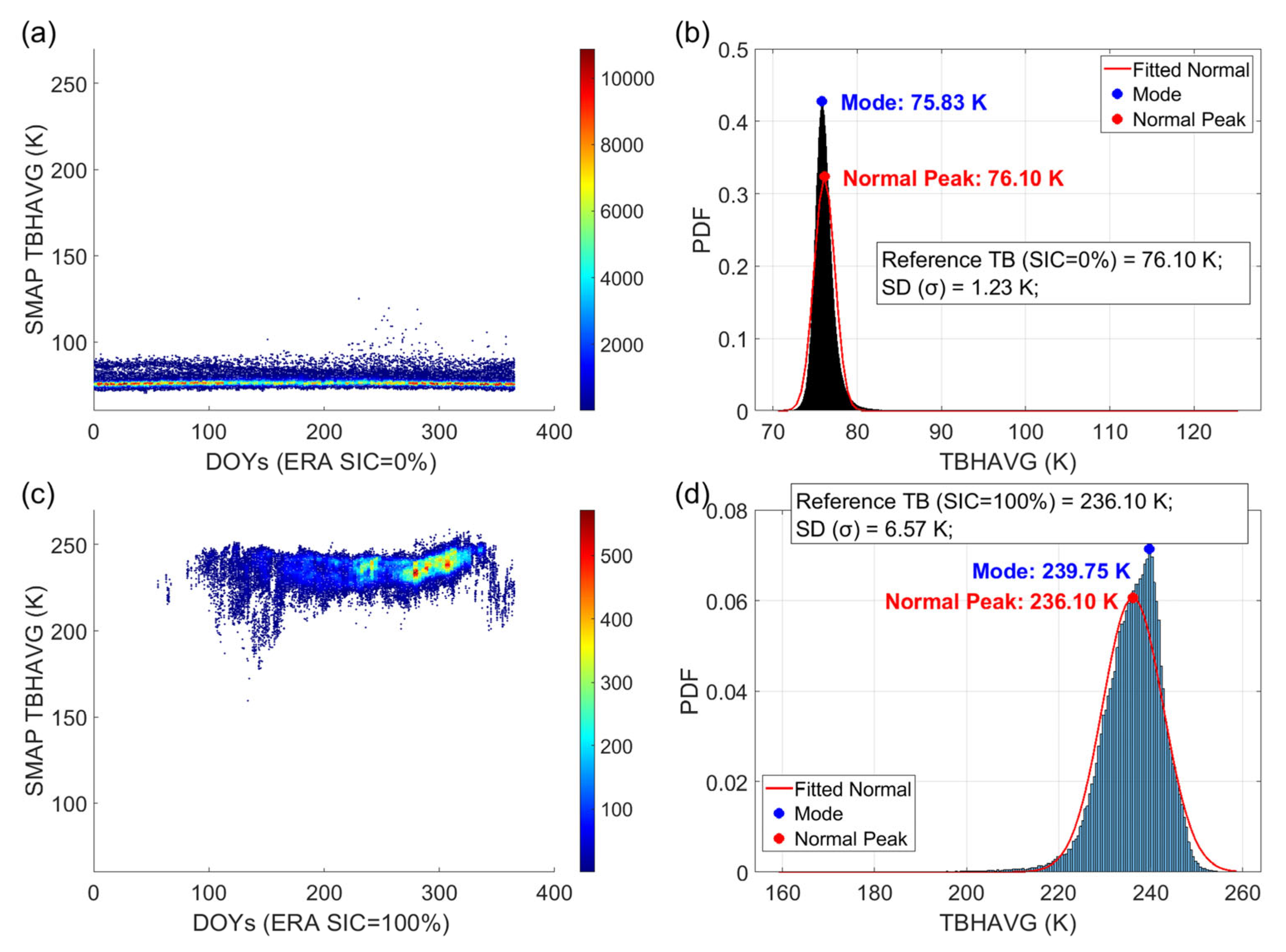
In Section 3.2, SST constraint of 278 K, IST constraint of 242 K, and DAV constraint of 1 K are determined to reduce the uncertainty of SIC retrieval. Although Arctic sea ice parameters (e.g., freeze–thaw timing, the proportion of multiyear ice) exhibit interannual variability, these thresholds in this study are determined using a large sample dataset covering the entire Arctic Ocean (on the order of 106 pixels per year). This extensive statistical space effectively smooths out fluctuations caused by local weather processes or single-year anomalies, thereby extracting robust signals representative of the typical climatic states of sea ice and sea surface temperatures. The study also considers the potential effect of an incomplete land mask. Therefore, the optimization process, which accounted for the four sources of uncertainty, necessitated the recomputation of the reference TB for both seawater and sea ice. For TBwater, the fluctuation range decreased from 70–200 K to 70–80 K after optimization. The standard deviation also reduced from 7.85 K to 1.23 K, as shown in Figure 9a,b. For TBice, the fluctuation range narrowed from 150–270 K to 230–250 K. Its standard deviation also decreased from 13.47 K to 6.57 K, as shown in Figure 9c,d. The lower variability of seawater TB may be explained by its dynamic balance and high heat capacity. Dynamic balance refers to the steady state maintained through the balance of heat absorption and release as well as phase-change processes, which reduces fluctuations in sea surface TB. In contrast, sea ice TB is more sensitive to differences in structure and composition. Besides, the clear separation between seawater and sea ice, as shown in the TB, further increases the reliability of the algorithm. Finally, the study determined the seawater and sea ice reference TB values to be 76.10 K and 236.10 K, respectively. These reference TB values are then substituted into the single-channel algorithm and Equations (4)–(6). This substitution yielded the final SIC retrieval equation, as expressed in Equation (10).
S I C = 0.63 × T B 47.5648

3.4. Justification for Using Single Horizontal Polarized TB as Core Input

To justify using SMAP horizontally polarized brightness temperature (TBH) as the sole input, we compare TBH, Polarization Ratio (PR), and Polarization Difference (PD) in distinguishing pure water and ice endmembers. Performance metrics included the mean difference (Δμ), relative standard deviation (RSD), and contrast-to-noise ratio (CNR). RSD is dimensionless, allowing dispersion comparison across signals. CNR provides an objective assessment of each signal’s classification potential and stability. The CNR is calculated as C N R = | μ w a t e r μ i c e | σ w a t e r 2 + σ i c e 2 .
The results indicate that, without considering uncertainties, TBH exhibits the best performance in terms of mean difference and RSD for ice (Table 2). After re-evaluating endmembers while accounting for uncertainties, TBH continues to demonstrate optimal performance across all metrics (Table 3). Specifically: Maximum mean difference between pure water and pure ice endmembers, indicating the strongest inherent discriminative ability. Minimum RSD within pure water and pure ice endmembers, displaying the most stable signal. Highest CNR, showing the most effective overall ability to distinguish the two types of endmembers. These statistical analyses clearly demonstrate that, for the SMAP dataset and research context in this study, the single SMAP TBH signal provides a more robust, low-noise, and discriminative basis for SIC retrieval than PR or PD.

4. Results

4.1. SIC Retrieval Results with Stepwise Uncertainty Treatments

4.1.1. Raw SIC Retrieval Without Any Uncertainty Mitigation

Figure 10 shows the reference TB of seawater and sea ice obtained without applying any uncertainty treatment. These reference brightness temperatures are used in the single-channel algorithm to retrieve L-band SIC, as shown in Equation (7). The scatter plot displays the overall distribution of L-band SIC versus SSM/I SIC. The density plot illustrates the concentration of points around the 1:1 reference line. It indicates the overall RMSE; the marginal histograms at the top and right show the distributions of the two SIC datasets. From Figure 10, it is evident that many scatter points deviate from the 1:1 reference line. This deviation reflects a systematic Bias in L-band SIC when uncertainties are not processed. Specifically, L-band SIC shows a negative Bias relative to the SSM/I SIC product. The overall RMSE is 10.51%, and the correlation coefficient R is 0.92. This suggests that the retrieval results can still capture the general distribution of sea ice, even without accounting for uncertainties. However, large errors and Biases persist, underscoring the need for subsequent uncertainty reduction and optimization to enhance accuracy.

4.1.2. SIC Retrieval After Removing Only the Uncertainties of TBwater

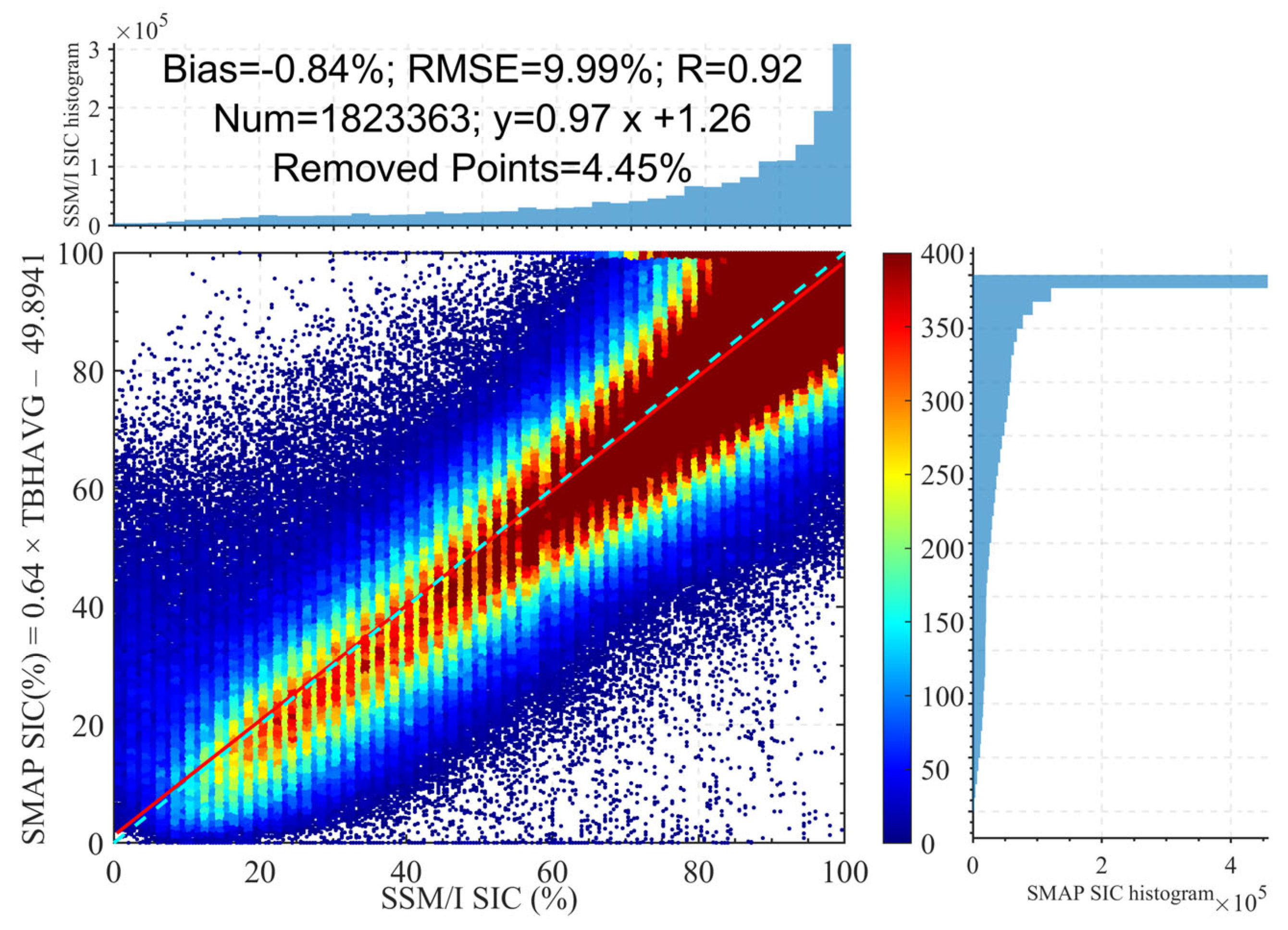
Corresponding to the discussion of TBwater uncertainty in Section 3.2.1, only ERA5 reanalysis data are used to constrain the SST. Specifically, when the ERA5 SST exceeds 278 K, the corresponding ERA5 SIC is set to 0%. Based on this, for grid points with ERA5 SIC equal to 0 but SST below 278 K, these abnormal samples are directly removed. After removing the abnormal samples, the TBwater is recalculated to retrieve SIC. When evaluating retrieval accuracy using SSM/I SIC, the same abnormal SST samples are excluded. The results are shown in Figure 11. Most points are concentrated near the 1:1 reference line, especially in the low-concentration range of SIC between 0% and 20%. The previously noticeable “hook” feature in this low-concentration region is largely weakened. Accordingly, the overall RMSE decreases from 10.51% to 9.99%. These results indicate that removing abnormal SST samples effectively reduces SIC retrieval errors and enhances the reliability in low-concentration regions.

4.1.3. SIC Retrieval After Removing Only the Uncertainties of TBicer

Corresponding to the discussion of TBicer uncertainty in Section 3.2.2, only the surface ice temperature (0–7 cm) provided by ERA5 is used as a constraint. Specifically, for grid points where the ERA5 ice temperature is below 242 K, these abnormal samples are directly removed. After removing the abnormal samples, the TBice is recalculated to retrieve SIC. When evaluating retrieval accuracy using SSM/I SIC, the same low-temperature abnormal points are excluded. Figure 12 shows that after removing the low-temperature points, Bias slightly decreases from −0.68 to −0.67. RMSE decreases from 10.51% to 10.50% after this removal. Compared with the impact of TBwater uncertainty on SIC, the uncertainty of TBice has a smaller effect on SIC.

4.1.4. SIC Retrieval After Removing Only the Uncertainties of DAV Signals Caused by Sea Ice Freeze–Thaw

Corresponding to the discussion in Section 3.2.3 on the impact of DAV signals reflecting sea ice freeze–thaw on SIC retrieval uncertainty, this study removes grid points with DAV > 1 K. This ensures that the remaining TB variations primarily reflect non-local freeze–thaw disturbances. After removing the high DAV points, new sea ice and seawater reference TB values are obtained for SIC retrieval. When evaluating retrieval accuracy using SSM/I products, these abnormal samples are also excluded. Figure 13 shows that most points in the density plot fall within the linear TB range. The contribution of off-linear points to RMSE is largely reduced. Especially in the 0–80% SIC range, points that originally deviated from the linear trend become more concentrated near the linear relationship after removal. Corresponding metrics indicate that Bias shifts from negative to positive. RMSE decreases by approximately 2 K. The correlation coefficient R increases from 0.92 to 0.94. These results indicate that DAV is a significant factor contributing to the increase in RMSE. Removing extreme DAVs stabilizes the linear relationship between SIC and TB. However, in the low-concentration regions of SSM/I SIC, L-band SIC still shows slight overestimation. This forms a “hook-shaped” pattern in the low-concentration region.

4.1.5. SIC Retrieval After Removing Only the Uncertainties of Incomplete Land Masking

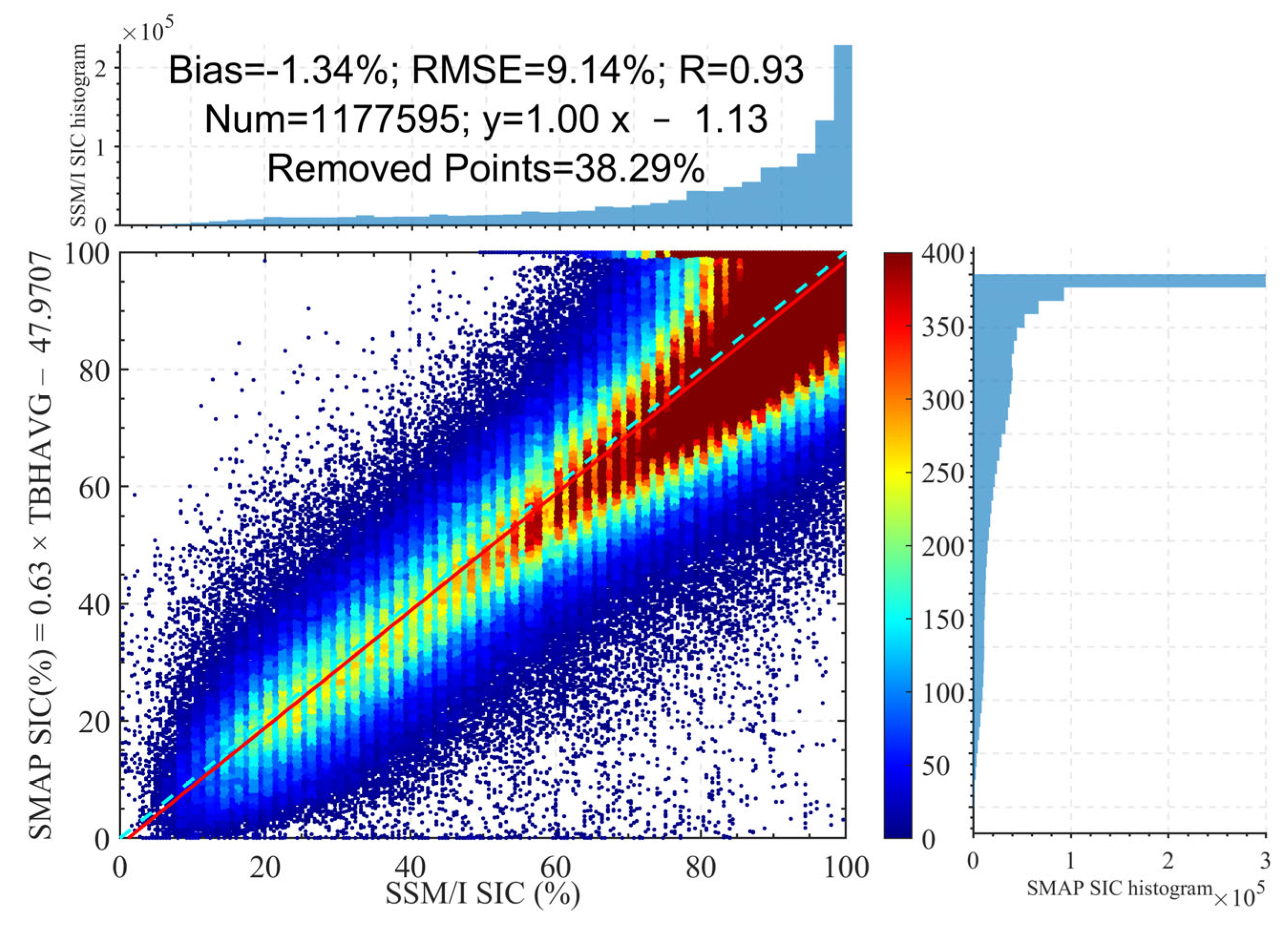
Corresponding to Section 3.2.4, this study analyzes the impact of incomplete land masking on SIC retrieval by comparing SIC results before and after applying a 1° buffered land mask. After further reducing the study area, Figure 14 shows that the previously evident “hook-shaped” pattern in the low-concentration region of SSM/I SIC versus SMAP SIC is effectively removed. This indicates that land interference on SIC primarily occurs in areas of low concentration. The corresponding density plot shows that after applying the buffered land mask, the scattered points are more concentrated. RMSE decreases from 10.51% to 9.14%. The correlation coefficient R increases. These results indicate that extending the masked land area can effectively reduce this interference.

4.1.6. Final SIC Retrieval After Removing Uncertainties of TBwater, TBice, DAV, and Incomplete Land Masking

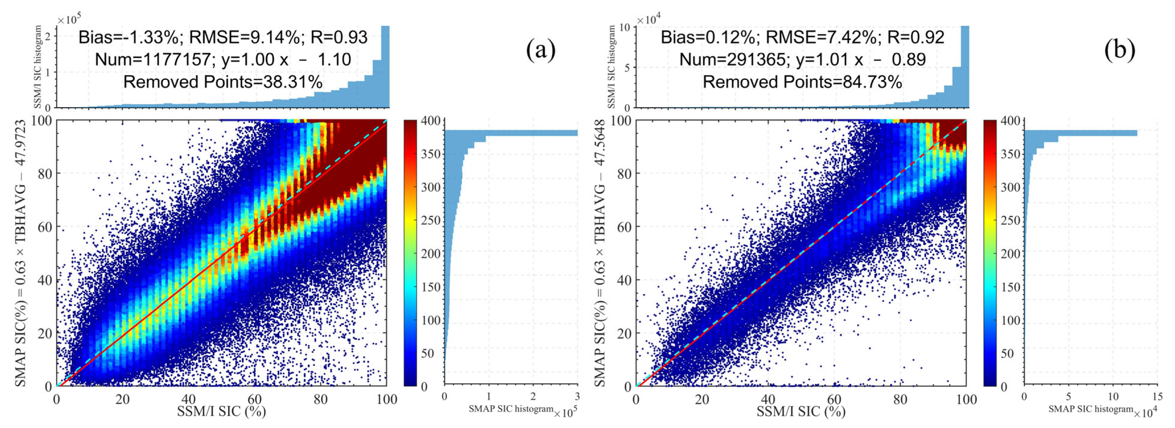
In Section 4.1.1, Section 4.1.2, Section 4.1.3, Section 4.1.4 and Section 4.1.5, after only removing samples with DAV > 1 K (Figure 13), Bias, RMSE, and R outperform other uncertainty treatments, indicating that the DAV signal largely affects the reference TB and the linear relationship between SIC and TB. Moreover, these uncertainty treatments strictly adhere to the core physical definition and applicable boundaries of SIC: land pixels, persistent open water, and perennial ice pixels are physically unsuitable for SIC retrieval or validation. Removing these samples focuses the analysis on the algorithm’s core target scenarios: sea ice marginal zones, seasonal ice regions, and areas experiencing freeze–thaw cycles. These steps constitute a physically justified sample selection based on prior knowledge, rather than a post hoc “optimization.” As shown in Figure 15, removing only the pixels unsuitable for SIC retrieval (approximately 38.3%) reduces RMSE from 10.51% to 9.14%, differing by less than 1% from removing only DAV and less than 2% from removing all uncertainties simultaneously. These results further support the hypothesis that the freeze–thaw process of sea ice largely affects SIC retrieval accuracy, an effect neglected by many conventional algorithms. Understanding the influence of freeze–thaw cycles, as reflected in DAV, helps further optimize SIC retrieval workflows and improve algorithm applicability and accuracy. Figure 15b shows that after removing all four types of uncertainties, the points cluster tightly around the 1:1 reference line, and nonlinear and low-concentration “hook” patterns are effectively removed; RMSE drops to 7.42%.

4.1.7. Stepwise Optimization and Error Reduction

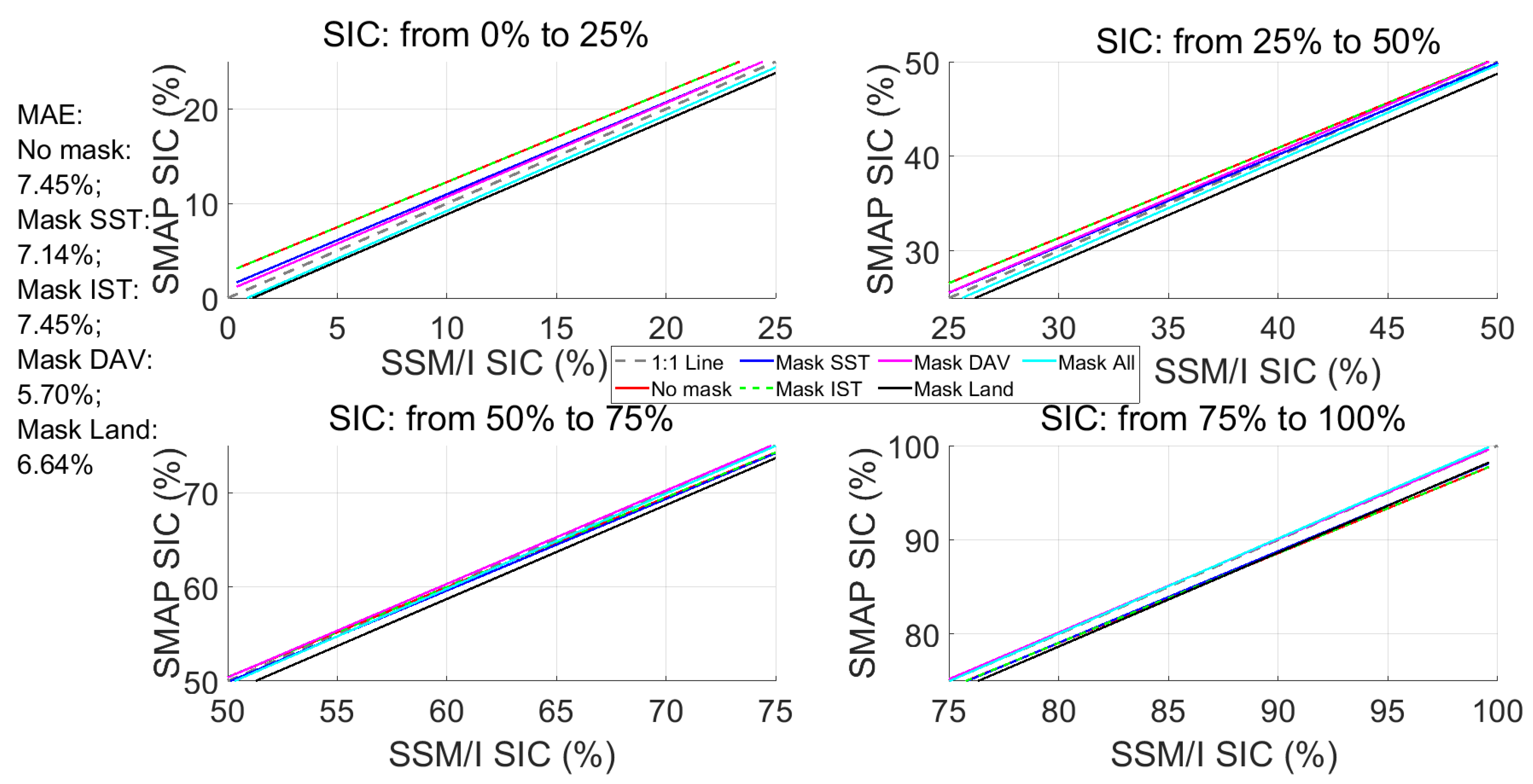
Optimization in this study essentially adjusts the algorithm’s response to different surface types (water, ice, transition zones) within a linear retrieval framework. Figure 16 illustrates this stepwise optimization, showing the algorithm results against the 1:1 line of reference data. Adjusting a single parameter corrects one direction in the multidimensional error space, which may temporarily worsen the fit in other regions. For example, the SST constraint primarily targets low SIC (<50%) to eliminate “overestimation” caused by warm water; this reduces positive Bias in low SIC areas but has little to no effect at higher SIC, sometimes increasing overall Bias (Figure 11). Applying the Land Mask removes pixels affected by coastal “spillover,” thereby eliminating strong positive bias. Any slight negative Bias in remaining ocean pixels may then appear more pronounced (Figure 14). Despite intermediate fluctuations in Bias, the fit line aligns better with the ideal 1:1 across mid-to-high SIC. MAE also decreases progressively: after SST and Land Mask, MAE improves from 7.45 to 7.14 and 6.64, respectively, indicating that absolute errors shrink and overall algorithm accuracy steadily improves.

4.2. Monthly Tests for Algorithm Robustness Assessment

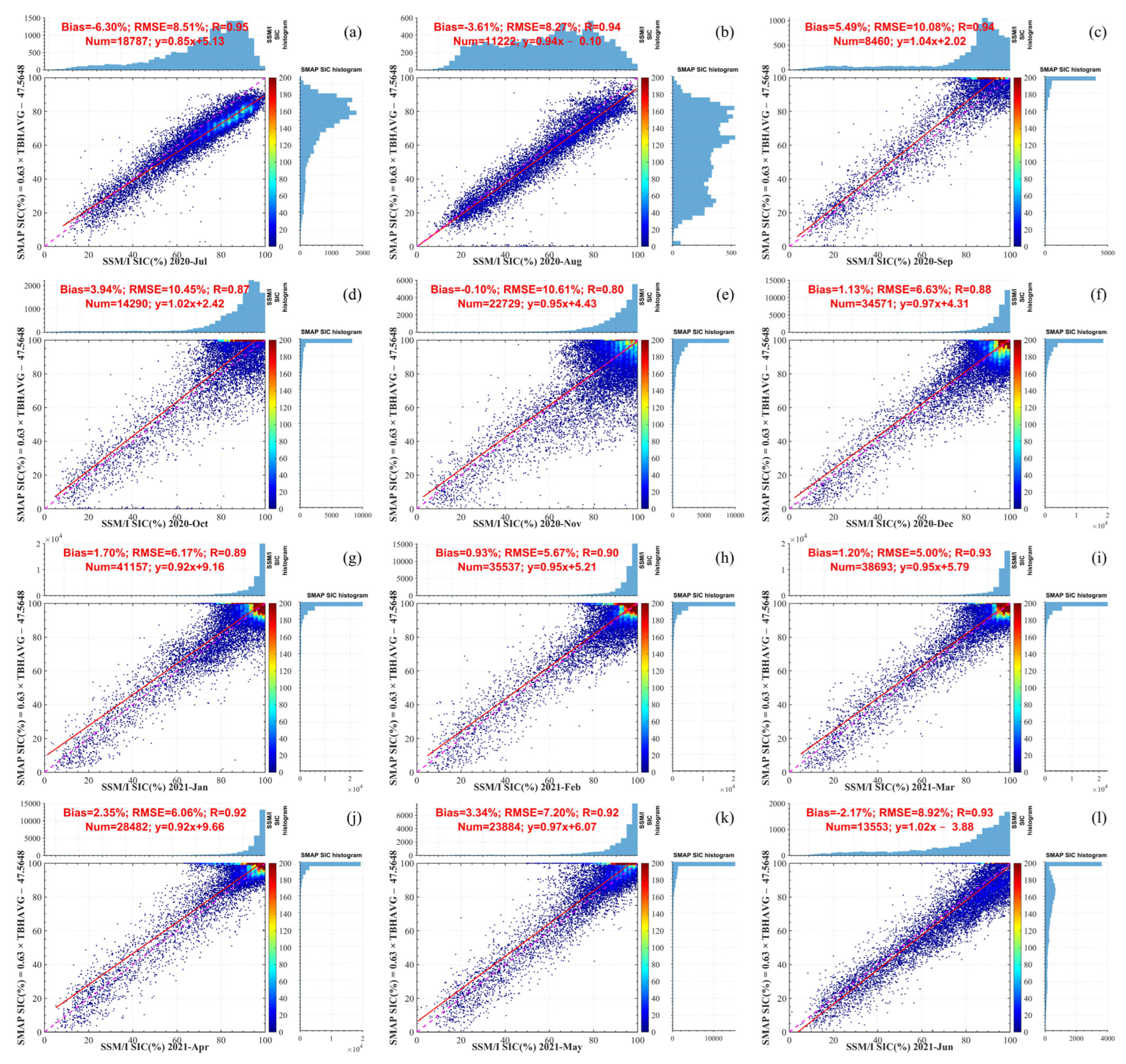
Based on Equation (10) and Figure 15, simultaneous removal of all four types of uncertainty yields an L-band SIC retrieval. Then the final SIC retrieval algorithm is applied to monthly evaluations throughout the year. As shown in Figure 17, summer warming causes sea ice to melt. This results in a more uniform SIC distribution. Consequently, SIC values range between 0% and 100%. Winter’s low temperatures promote the formation and accumulation of sea ice. As a result, sea ice coverage expands, and SIC values are generally close to 100%. Among the 12 months, only June, July, and August exhibit a negative Bias. During the freeze–thaw transition periods in May and September, as well as in the remaining seven months, Bias is positive. This indicates that, after removing abnormal points caused by all types of uncertainties, especially local sea ice freeze–thaw, L-band SIC tends to overestimate SSM/I SIC overall by a slight margin. The accuracy of winter SIC retrieval is higher than that of summer. Both Bias and RMSE are reduced mainly in winter. This high accuracy is particularly evident in February and March 2021. During these months, Bias is around 1% and RMSE is around 5%. High winter accuracy may result from the more stable environment during winter. The stable environment allows the algorithm to reliably identify TB, reducing systematic deviations caused by environmental factors. Additionally, the correlation between the two products is significantly lower in winter than in summer and in the annual average. This difference may result from the limited number of effective winter observations and the highly concentrated SIC distribution. Most winter observations are focused on high-concentration ranges. This limits the responsiveness of statistical regression models under different concentration conditions. Overall, analysis of the 12-month R values shows that they are mostly above 0.9. RMSE values are mostly below 10%. Bias values are mostly below 5%.

4.3. Seasonal Variability of New L-Band Algorithm SIC and SSM/I SIC

As for the validation in Section 4.3, Section 4.4 and Section 4.5, pixels are removed only according to the four sources of uncertainty defined during endmember selection (Equation (10)). Unlike in Section 4.1 and Section 4.2, no pixels are removed during the validation process itself. When evaluating large-area gridded products (Section 4.1 and Section 4.2), physical filtering enables the assessment of the algorithm’s performance in “advantageous regions.” In contrast, the seasonal variability, shipborne, and SAR validation (Section 4.3, Section 4.4 and Section 4.5) provide an unfiltered view of the algorithm’s overall performance in real-world conditions, including challenging areas. The combination of these two approaches fully characterizes the algorithm’s performance.
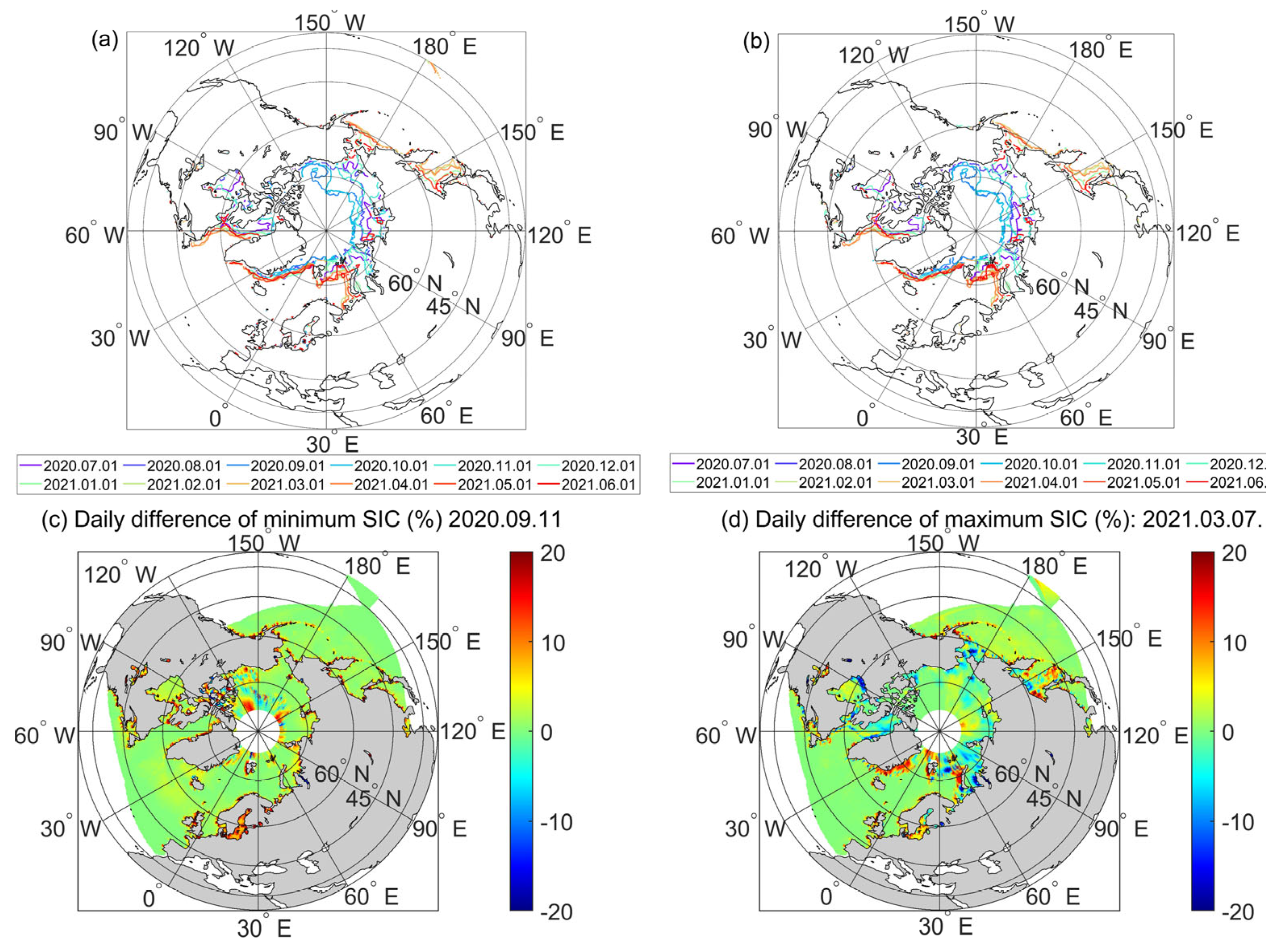
As shown in Figure 18a,b, the 15% SIC contour illustrates the seasonal contraction and expansion of sea ice. During winter (December 2020 to March 2021), both SIC products indicate sea ice expansion. During the summer (September to October 2020), SIC clearly contracts. On days with the daily minimum ice extent, which is derived from L-band SIC (Figure 18c), L-band SIC is slightly higher than SSM/I SIC in most regions. However, the overall difference is negligible. These deviations may reflect differences in how the algorithms respond to physical processes of sea ice. During summer, the sea ice surface often contains meltwater or coexisting freeze–thaw states. Different microwave frequencies react differently to these states. Among them, the L-band is more sensitive to liquid water on the ice surface. On days with the daily maximum ice extent (Figure 18d), L-band SIC is lower than SSM/I SIC near land boundaries. This discrepancy may result from land influence, as the study region is not adjusted for in this section. Overall, despite being based on different frequency bands, L-band SIC and SSM/I SIC show high consistency in seasonal variations and regional scales. The differences mainly arise from how the other bands respond to physical processes and local environmental conditions.

4.4. Validation Against Ship-Based SIC Observations

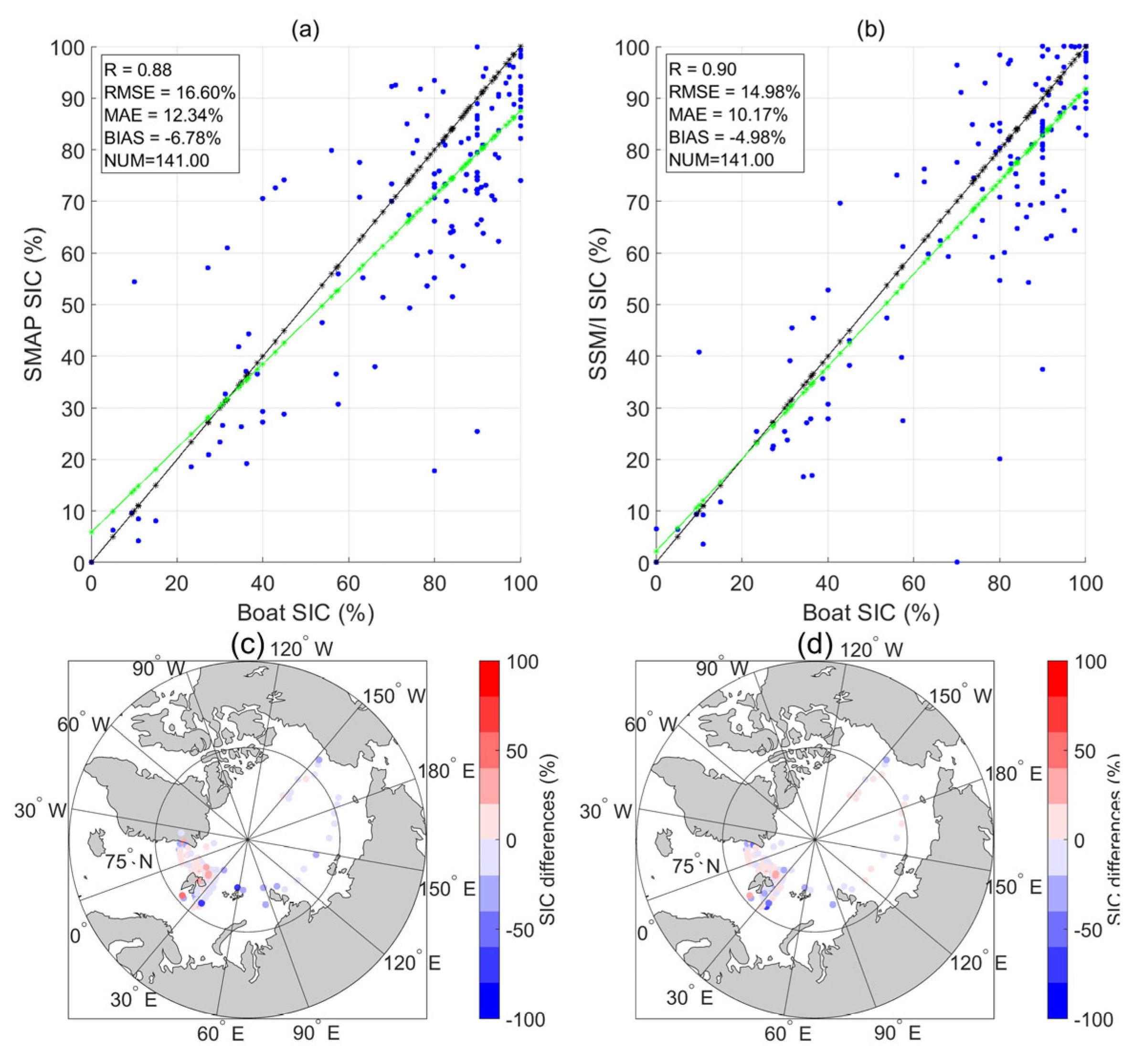
To further assess the reliability of the new L-band SIC retrieval algorithm, the SIC obtained from Equation (10) is compared with in situ measurements made on board ships. Figure 19a shows that under low SIC conditions, L-band retrieval agrees well with ship observations. Under high SIC conditions, the L-band retrieval slightly underestimates SIC. The average Bias is approximately 6.78%. RMSE is 16.60%, and the MAE is 12.34%.
In comparison, the SSM/I product exhibits a more balanced performance across all SIC levels (Figure 19b). Its Bias, RMSE, and MAE are lower than those of the L-band retrieval by roughly 2%, 2%, and 2%, respectively. It should be noted that the spatial scale mismatch between ship-based observations (with a typical visual radius of ~1 km) and SMAP L-band observations (with a resolution of ~36 km) can introduce significant representativeness errors, particularly in regions with high sea ice heterogeneity, such as the marginal ice zone. This is a well-recognized challenge in validating passive microwave SIC products. Therefore, the reported RMSE should be interpreted as a measure of agreement between the SMAP or SSM/I SIC product and ship-based point measurements under the realistic condition of inherent scale disparity. Overall, although the SMAP L-band product has a spatial resolution of 36 km × 36 km, which is lower than the 25 km × 25 km of SSM/I, the accuracies of the two products are comparable. Figure 18c,d show that the largest SIC retrieval differences are located in the Greenland Sea. In other regions, the two satellite products are highly consistent. These results demonstrate that the new L-band SIC retrieval algorithm is reliable and robust for practical applications.

4.5. Validation Against SAR SIC Observations

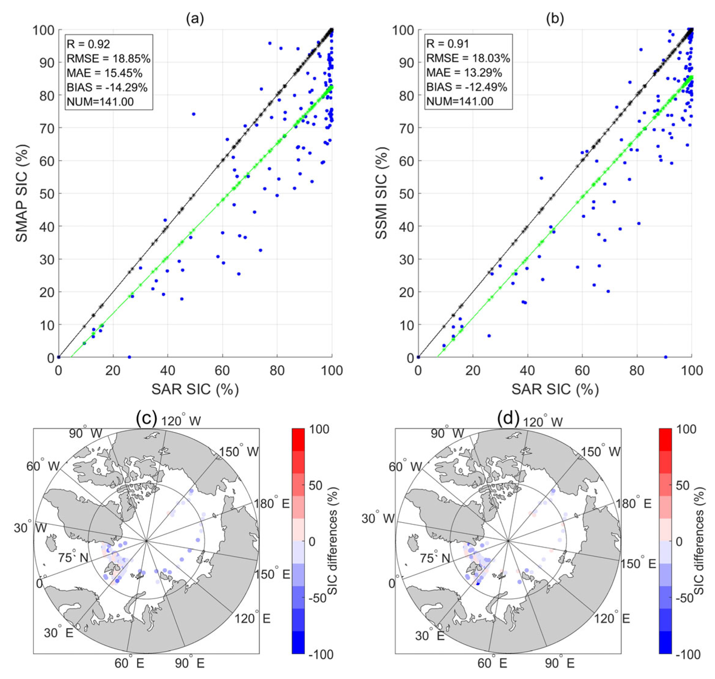
In this section, SAR SIC (see Section 2.4) is incorporated. Comparison with SAR shows that under low SIC conditions, the L-band retrieval agrees well with SAR, while under high SIC conditions, it is slightly lower than SAR, with an average Bias of approximately –14.29%, RMSE of 18.85%, and MAE of 15.45% (Figure 20a). Bias, RMSE, and MAE are approximately 2%, 1%, and 2% higher than those of SSM/I, respectively, while the correlation coefficient reaches 0.92, slightly higher than 0.91 between SSM/I and SAR SIC (Figure 20b). Although the SMAP spatial resolution (36 km × 36 km) is coarser than that of SSM/I (25 km × 25 km), it still maintains good accuracy and stability. Figure 20c,d show localized overestimation near Greenland, while most areas are underestimated. These results indicate that the algorithm performs similarly to SSM/I when validated against in situ and SAR data, both in core regions and in more challenging real-world scenarios.

5. Discussion

5.1. Linking DAV Signal to the Sea-Ice Surface Freeze–Thaw Process

This section provides direct observational evidence showing that the periodic L-band DAV anomalies are characteristic signals of the diurnal freeze–thaw cycle on the sea-ice surface, which can be effectively distinguished from other surface processes. First, the 1.4 GHz L-band radiometer has a strong atmospheric penetration capability, and attenuation by atmospheric components (oxygen, water vapor, and cloud liquid water) is significantly lower than at higher microwave frequencies [46,61,62]. Diurnal variations in water vapor are insufficient to produce the persistent, quasi-daily oscillations observed. Besides, wind-induced changes in ice surface roughness typically occur as discrete events, often associated with weather systems or the passage of mesoscale cyclones [63]. The wind field over sea ice lacks predictable patterns capable of driving spatially coherent daily oscillations, so changes in roughness caused by wind also cannot account for the continuous DAV signal observed.
Second, snow-related physical processes cannot generate the specific, persistent, and phase-consistent periodic DAV signal observed in this study. Once snow melts, its density, structure, and liquid water content are permanently altered, and it does not fully refreeze overnight. As a result, snow typically produces only short-term step changes or transient spikes in the DAV signal, rather than recurring daily oscillations. Previous studies [64,65] have shown that melting snow at 36.5 GHz can induce a brief DAV enhancement; however, subsequent refreezing or further melting does not produce sustained cycles. Snow-related effects typically result in only a single, short-lived enhancement within a year.
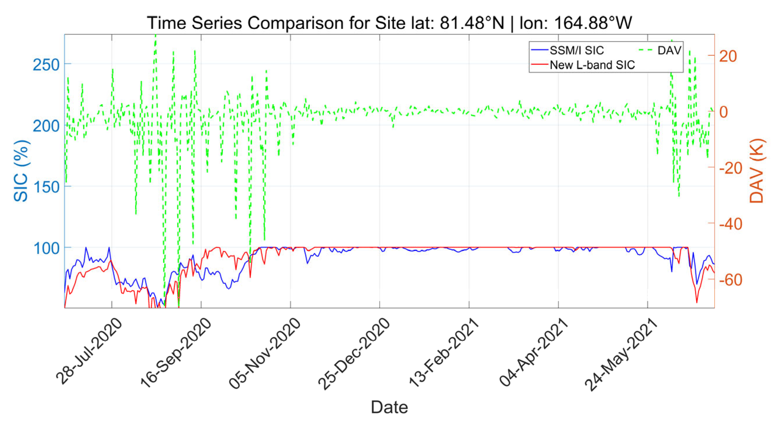
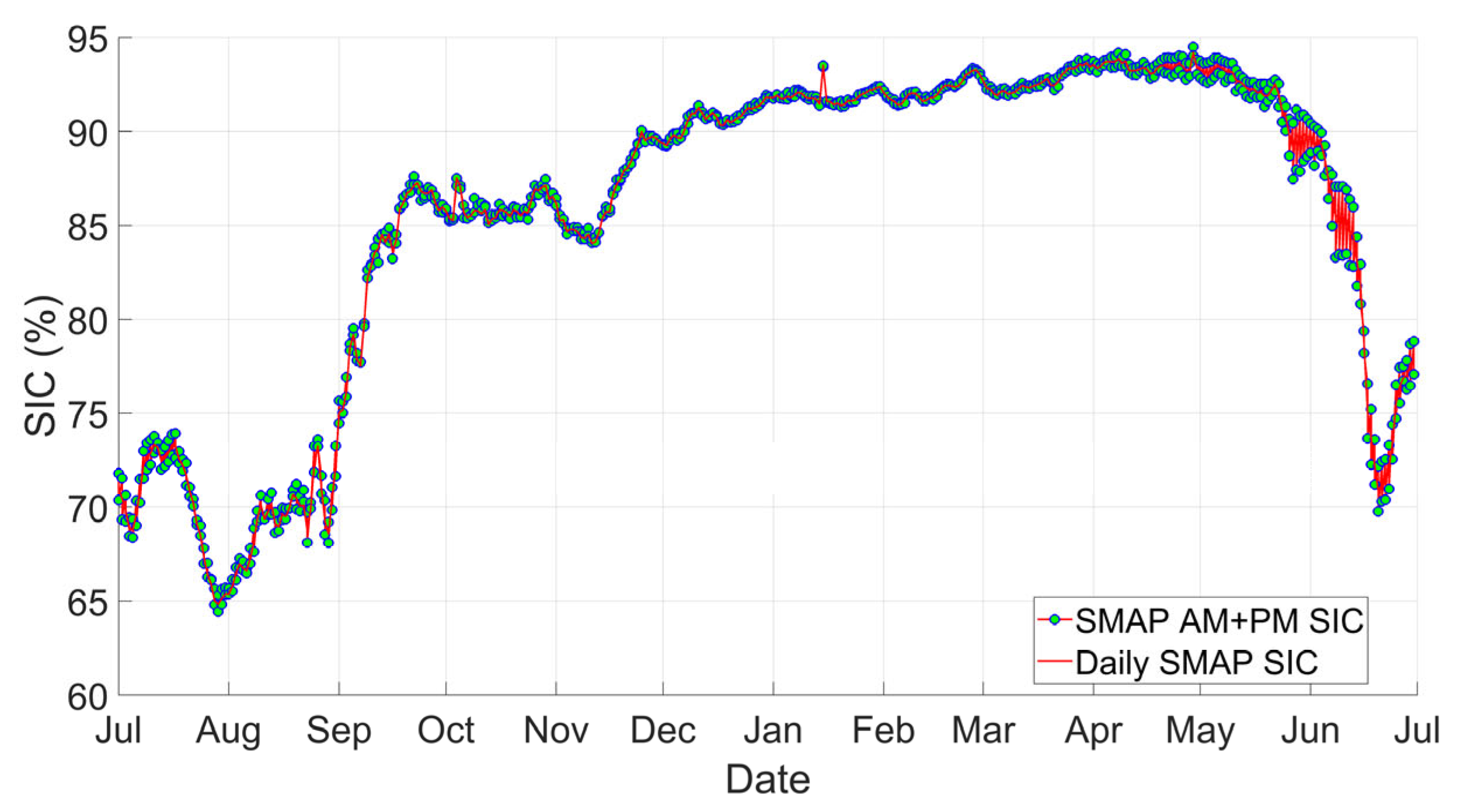
In contrast, L-band DAV represents the diurnal amplitude of TB, which is determined by surface emissivity and physical temperature (Equation (2)). Theoretically, according to Equations (8) and (9), DAV should be smaller than the corresponding diurnal variation in physical temperature. However, during melting, part of the ice converts to water, and the coexistence of ice and water alters the effective surface emissivity, thereby modifying the observed TB [43]. Therefore, if it is observed that DAV exceeds the expected range, it indicates that the sea ice may be undergoing a freeze–thaw process. To support this interpretation, Figure 21 presents a time series of L-band (1.41 GHz) DAV at a representative location (green dashed line), alongside SIC retrieved by the new L-band algorithm (red line) and SSM/I SIC (blue line). The time series shows that DAV undergoes continuous, quasi-daily oscillations during the transition period, with phase coherence and repeated cycling clearly distinct from random snowfall or melt events, which cannot produce such regular temporal patterns over comparable timescales.

5.2. Advantage of DAV Signal

In this study, a new sea-ice concentration (SIC) retrieval framework based on multi-physical constraint collaborative optimization is proposed, which integrates sea-surface temperature, ice-surface temperature, a land mask, and introduces the L-band DAV as a dynamic physical constraint. The inclusion of DAV is not only intended to improve SIC retrieval accuracy but also to reveal the physical limitations of the conventional SIC definition. For instance, under the traditional definition, a 20% SIC does not distinguish between “pure ice” and “ice containing liquid water.” In the latter case, the ice–water mixture may still be observed as 20% SIC by passive microwave sensors, while the actual surface state has undergone a physical change. DAV captures such state changes and also highlights that conventional retrieval workflows often fail to account for surface phase transitions [26] fully. Therefore, discussions of “accuracy” must consider the SIC definition itself. Even if a retrieval model produces values consistent with others, it cannot negate the physical information and reality revealed by DAV when freeze–thaw dynamics are occurring.
Therefore, in this study, DAV itself is a high-value geophysical signal, directly indicating whether the sea-ice surface is undergoing intense diurnal freeze–thaw cycles. It is essential to clarify the role of DAV in our methodology. The exclusion of pixels with DAV > 1 K was strictly limited to the algorithm development and endmember selection phase (Section 3.2, Section 4.1 and Section 4.2). This temporary measure ensured the derivation of stable reference brightness temperatures. It was not applied in the final retrieval or validation (Section 4.3, Section 4.4 and Section 4.5). For these final steps, the fully trained algorithm is applied to all pixels without exclusion. Consequently, in these processes, the high-DAV condition itself is then actively used as the criterion for flagging, adding a “surface state stability” quality-control layer to the SIC product. This allows users to distinguish between regions of stable ice–water mixtures and dynamically changing surfaces undergoing phase transitions—a capability vital for accurately interpreting SIC data and improving the parameterization of surface energy fluxes in sea-ice–climate coupled models. It also provides a reference for subsequent efforts to fuse SMAP with high-frequency SIC data to enhance spatial resolution. As shown in Figure 22, by applying Equation (10) separately to ascending/descending TB observations, two SIC results can be obtained for the same day, thereby capturing the diurnal variability of L-band SIC. This approach maps ascending and descending temperature differences into the SIC retrieval, transforming the smoothed daily mean SIC into SIC with intra-day fluctuations that reflect the dynamic state of sea ice during the freeze–thaw transition and summer, a feature that most existing algorithms fail to capture. Although the spatial resolution of SMAP L-band (36 km × 36 km) is lower than that of SSM/I (25 km × 25 km), its SIC retrieval maintains good stability. It performs comparably to SSM/I, making it suitable for large-scale climate simulations while reducing computational costs.

5.3. Application and Limitations of ERA5 SIC in Endmember Definition

In this study, pure water and sea ice endmembers are defined using ERA5 SIC. ERA5 SIC is an optimally reanalyzed product that integrates multi-source observations and exhibits good spatiotemporal continuity, rather than a single direct observation with unknown errors. In the absence of long-term, global, and unbiased “true” observational data, using it to define endmembers over large areas is reasonable. However, ERA5 has limitations [49]: polar ice temperatures exhibit a warm bias, extreme sea surface temperatures have higher uncertainty, and SIC derived from reanalysis may be affected by observational errors and assimilation system biases, especially in regions with high mixed pixels or rapidly evolving ice. Therefore, defining endmembers inevitably introduces inherent uncertainties from the reanalysis, which must be fully considered in subsequent applications.

5.4. Challenges in Obtaining Validation Data

During optimization and evaluation, the SSM/I product from the NASA Team’s algorithm is used as a benchmark, as it is a long-established and widely applied product. To enhance independence and comprehensiveness of validation, ship-based observations and high-resolution SAR data are also incorporated. Nevertheless, the SSM/I product has known limitations, including weather effects, surface emissivity variations, and biases during the melt season, meaning its consistency reflects relative rather than absolute truth [10]. Moreover, validating SIC remote sensing products is inherently challenging, as different products vary, and large-scale, long-term, and continuous ground truth is lacking. Therefore, future studies should emphasize multi-source cross-validation to improve the accuracy of SIC products and provide a more reliable framework for long-term sea-ice monitoring.

5.5. Impact of Sea Ice Thickness

In reality, thin-ice regions often exhibit high spatial heterogeneity and rapid dynamics (e.g., fragmented ice, mixed pixels, convergence/divergence) [66], meaning the impact of SIC changes within a pixel on TB is generally larger than thickness variations of several tens of centimeters. The new L-band algorithm in this study focuses on SIC retrieval, capturing emissivity changes caused by the ice-to-water fraction, and explicitly assumes that secondary effects from ice thickness are negligible, a common simplification in most SIC algorithms. However, the thicknesses of ice may introduce additional errors. Therefore, future work can incorporate independent ice thickness products (e.g., altimetry or high-resolution SAR) as auxiliary information to improve retrievals over thin-ice areas.

6. Conclusions

This study demonstrates the potential of retrieving SIC from L-band TB observations and systematically analyzes four key uncertainties in the retrieval algorithm. These uncertainties are: (1) variations in seawater reference TB under warm water conditions, (2) variations in sea ice reference TB under extremely low-temperature conditions, (3) the freeze–thaw dynamics of sea ice captured by DAV signals, and (4) land mask imperfections. These uncertainties are quantified and constrained by determining the optimal threshold and then formulating an SIC retrieval algorithm under idealized conditions. The main conclusions are as follows:
(1)
Compared to SSM/I SIC, DAV has the most significant influence on the accuracy of the SIC retrieval algorithm. By eliminating the uncertainties of DAV caused by sea ice freeze–thaw processes, RMSE decreases from 10.51% to 8.43%, and R improves from 0.92 to 0.94. Bias value also decreases from −0.68% to 0.12%. After eliminating four uncertainties, a retrieval algorithm for SIC is established under ideal conditions. RMSE further reduces to 7.42% (approximately a 3% reduction). Besides, the difference between the algorithm and SSM/I SIC in winter is much smaller than that in summer. R values mostly exceed 0.9 for twelve months, RMSE is mostly below 10%, and Bias is mostly less than 5%. Consequently, both datasets reveal a high degree of consistency in capturing seasonal trends of sea ice contraction and expansion.
(2)
Compared to ship-based SIC data, the algorithm shows high accuracy and consistency, especially under low SIC conditions, even outperforming SSM/I. Bias, RMSE, and MAE are approximately 2%, 2%, and 2% higher than those of SSM/I SIC. The differences mainly appear in the Greenland Sea, while other areas show consistency.
(3)
Compared with ship measurements, the L-band and SSM/I satellites show slightly worse validation against SAR, with Bias, RMSE, and MAE about 2%, 1%, and 2% higher, respectively. Over Greenland, there may be localized overestimation, but most areas are underestimated.
Conventional SIC retrieval assumes constant sea-ice emissivity and dielectric properties, thereby ignoring changes that occur during melt. This study demonstrates that uncertainties, particularly those related to sea-ice freeze–thaw dynamics captured by DAV signals, have a significant impact on SIC retrieval. DAV itself is a high-value geophysical signal. It directly indicates whether the sea-ice surface is undergoing intense diurnal freeze–thaw cycles. By linking ascending and descending TB differences to SIC, DAV introduces diurnal variability, better representing instantaneous sea-ice states, particularly during summer and transition periods. Incorporating DAV provides a practical way to identify melt–refreeze processes and offers insights for large-scale SIC simulation, data assimilation, and understanding ice-atmosphere interactions.

Author Contributions

Conceptualization, Y.H., S.L. and Z.L.; methodology, Y.H.; software, Y.H.; validation, Y.H.; formal analysis, Y.H.; investigation, Y.H.; resources, Y.H. and S.L.; data curation, Y.H.; writing—original draft preparation, Y.H.; writing—review and editing, S.L., Z.L., Y.Z. (Yijian Zeng), X.L., Y.Z. (Yijun Zhang) and J.W.; visualization, Y.H. and S.L.; supervision, S.L., Z.L., Y.Z. (Yijian Zeng), X.L., Y.Z. (Yijun Zhang) and J.W.; project administration, Y.H. and S.L.; funding acquisition, S.L. All authors have read and agreed to the published version of the manuscript.

Funding

This research was funded by Inner Mongolia Science and Technology Program Project (No. 025YFDZ0007), the Key Research and Development and Achievement Transformation Program of Inner Mongolia Autonomous Region, China (Grant No. 2025YFDZ0007), the National Natural Science Foundation of China (Grant No. 42075150), the National Key R&D Program of China (Grant No. 2022YFF0801404), and the Yan Liyuan–ENSKY Foundation Project of Zhuhai Fudan Innovation Research Institute (Grant No. JX240002).

Data Availability Statement

This study was conducted using E.U. Copernicus Marine Service Information, specifically the SAR sea ice concentration (SIC) product, available at https://doi.org/10.48670/mds-00344 (accessed on 24 November 2025). SMAP brightness temperature data can be accessed at https://nsidc.org/data/spl3ftp/versions/3, accessed on 10 November 2023. SSM/I SIC data can be obtained from the NSIDC website (https://nsidc.org/data/nsidc-0051/versions/2, accessed on 15 June 2024). ERA5 data can be accessed at the ECMWF’s official website (https://cds.climate.copernicus.eu/datasets/reanalysis-era5-single-levels?tab=overview, accessed on 15 June 2024). Ship-based sea ice concentration (SIC) data can be accessed under the ICEWatch/ASSIST program in the Arctic (https://cryo.met.no/en/icewatch, accessed on 25 February 2025).

Acknowledgments

We sincerely appreciate all the contributors to the dataset used in this study.

Conflicts of Interest

The authors declare no conflicts of interest.

References

  1. Lei, R.; Tian-Kunze, X.; Leppäranta, M.; Wang, J.; Kaleschke, L.; Zhang, Z. Changes in summer sea ice, albedo, and portioning of surface solar radiation in the Pacific sector of Arctic Ocean during 1982–2009. J. Geophys. Res. 2016, 121, 5470–5486. [Google Scholar] [CrossRef]
  2. Hopsch, S.; Cohen, J.; Dethloff, K. Analysis of a link between fall Arctic sea ice concentration and atmospheric patterns in the following winter. Tellus A Dyn. Meteorol. Oceanogr. 2012, 64, 18624. [Google Scholar] [CrossRef]
  3. Gorodetskaya, I.V.; Cane, M.A.; Tremblay, L.B.; Kaplan, A. The effects of sea-ice and land-snow concentrations on planetary albedo from the earth radiation budget experiment. Atmos. Ocean 2006, 44, 195–205. [Google Scholar] [CrossRef]
  4. Meier, W.N.; Hovelsrud, G.K.; van Oort, B.E.H.; Key, J.R.; Kovacs, K.M.; Michel, C.; Haas, C.; Granskog, M.A.; Gerland, S.; Perovich, D.K.; et al. Arctic sea ice in transformation: A review of recent observed changes and impacts on biology and human activity. Rev. Geophys. 2014, 52, 185–217. [Google Scholar] [CrossRef]
  5. Struthers, H.; Ekman, A.M.L.; Glantz, P.; Iversen, T.; Kirkevåg, A.; Mårtensson, E.M.; Seland, Ø.; Nilsson, E.D. The effect of sea ice loss on sea salt aerosol concentrations and the radiative balance in the Arctic. Atmos. Chem. Phys. 2011, 11, 3459–3477. [Google Scholar] [CrossRef]
  6. Njoku, E.G. Passive microwave remote sensing of the earth from space—A review. Proc. IEEE 1982, 70, 728–750. [Google Scholar] [CrossRef]
  7. Tomiyasu, K. Remote sensing of the earth by microwaves. Proc. IEEE 1974, 62, 86–92. [Google Scholar] [CrossRef]
  8. Njoku, E.G.; Stacey, J.M.; Barath, F.T. The Seasat scanning multichannel microwave radiometer (SMMR): Instrument description and performance. IEEE J. Ocean. Eng. 1980, 5, 100–115. [Google Scholar] [CrossRef]
  9. Comiso, J.C. Enhanced Sea Ice Concentrations and Ice Extents from AMSR-E Data. J. Remote Sens. Soc. Jpn. 2009, 29, 199–215. [Google Scholar]
  10. Cavalieri, D.J.; Gloersen, P.; Campbell, W.J. Determination of sea ice parameters with the NIMBUS 7 SMMR. J. Geophys. Res. Atmos. 1984, 89, 5355–5369. [Google Scholar] [CrossRef]
  11. Comiso, J.C. Characteristics of Arctic winter sea ice from satellite multispectral microwave observations. J. Geophys. Res. Ocean. 1986, 91, 975–994. [Google Scholar] [CrossRef]
  12. Pedersen, L.T. Retrieval of Sea Ice Concentration by Means of Microwave Radiometry. Ph.D. Thesis, Technical University of Denmark, Kongens Lyngby, Denmark, 1991. [Google Scholar]
  13. Markus, T.; Cavalieri, D.J. An enhancement of the NASA Team sea ice algorithm. IEEE Trans. Geosci. Remote Sens. 2000, 38, 1387–1398. [Google Scholar] [CrossRef]
  14. Spreen, G.; Kaleschke, L.; Heygster, G.C. Sea ice remote sensing using AMSR-E 89-GHz channels. J. Geophys. Res. 2008, 113. [Google Scholar] [CrossRef]
  15. Chen, Y.; Zhao, X.; Pang, X.; Ji, Q. Daily sea ice concentration product based on brightness temperature data of FY-3D MWRI in the Arctic. Big Earth Data 2022, 6, 164–178. [Google Scholar] [CrossRef]
  16. Zhao, X.; Chen, Y.; Kern, S.; Qu, M.; Ji, Q.; Fan, P.; Liu, Y. Sea Ice Concentration Derived From FY-3D MWRI and Its Accuracy Assessment. IEEE Trans. Geosci. Remote Sens. 2022, 60, 4300418. [Google Scholar] [CrossRef]
  17. Tonboe, R.T.; Nandan, V.; Mäkynen, M.; Pedersen, L.T.; Kern, S.; Lavergne, T.; Øelund, J.; Dybkjær, G.; Saldo, R.; Huntemann, M. Simulated Geophysical Noise in Sea Ice Concentration Estimates of Open Water and Snow-Covered Sea Ice. IEEE J. Sel. Top. Appl. Earth Obs. Remote Sens. 2022, 15, 1309–1326. [Google Scholar] [CrossRef]
  18. Lu, J.; Scarlat, R.; Heygster, G.; Spreen, G. Reducing Weather Influences on an 89 GHz Sea Ice Concentration Algorithm in the Arctic Using Retrievals from an Optimal Estimation Method. J. Geophys. Res. Ocean. 2022, 127, e2019JC015912. [Google Scholar] [CrossRef]
  19. Lavergne, T.; Sørensen, A.M.; Kern, S.; Tonboe, R.; Notz, D.; Aaboe, S.; Bell, L.; Dybkjær, G.; Eastwood, S.; Gabarro, C.; et al. Version 2 of the EUMETSAT OSI SAF and ESA CCI sea-ice concentration climate data records. Cryosphere 2019, 13, 49–78. [Google Scholar] [CrossRef]
  20. Wang, L.; Scott, K.A.; Clausi, D.A. Sea Ice Concentration Estimation during Freeze-Up from SAR Imagery Using a Convolutional Neural Network. Remote Sens. 2017, 9, 408. [Google Scholar] [CrossRef]
  21. Cooke, C.L.V.; Scott, K.A. Estimating Sea Ice Concentration From SAR: Training Convolutional Neural Networks with Passive Microwave Data. IEEE Trans. Geosci. Remote Sens. 2019, 57, 4735–4747. [Google Scholar] [CrossRef]
  22. Chi, J.; Kim, H.-c.; Lee, S.; Crawford, M.M. Deep learning based retrieval algorithm for Arctic sea ice concentration from AMSR2 passive microwave and MODIS optical data. Remote Sens. Environ. 2019, 231, 111204. [Google Scholar] [CrossRef]
  23. Ivanova, N.; Pedersen, L.T.; Tonboe, R.T.; Kern, S.; Heygster, G.; Lavergne, T.; Sørensen, A.; Saldo, R.; Dybkjær, G.; Brucker, L.; et al. Inter-comparison and evaluation of sea ice algorithms: Towards further identification of challenges and optimal approach using passive microwave observations. Cryosphere 2015, 9, 1797–1817. [Google Scholar] [CrossRef]
  24. Ivanova, N.; Johannessen, O.M.; Pedersen, L.T.; Tonboe, R.T. Retrieval of Arctic Sea Ice Parameters by Satellite Passive Microwave Sensors: A Comparison of Eleven Sea Ice Concentration Algorithms. IEEE Trans. Geosci. Remote Sens. 2014, 52, 7233–7246. [Google Scholar] [CrossRef]
  25. Kattsov, V.M.; Ryabinin, V.E.; Overland, J.E.; Serreze, M.C.; Visbeck, M.; Walsh, J.E.; Meier, W.; Zhang, X. Arctic sea-ice change: A grand challenge of climate science. J. Glaciol. 2010, 56, 1115–1121. [Google Scholar] [CrossRef]
  26. Kern, S.; Lavergne, T.; Notz, D.; Pedersen, L.T.; Tonboe, R. Satellite passive microwave sea-ice concentration data set inter-comparison for Arctic summer conditions. Cryosphere 2020, 14, 2469–2493. [Google Scholar] [CrossRef]
  27. Kern, S.; Lavergne, T.; Notz, D.; Pedersen, L.T.; Tonboe, R.T.; Saldo, R.; Sørensen, A.M. Satellite passive microwave sea-ice concentration data set intercomparison: Closed ice and ship-based observations. Cryosphere 2019, 13, 3261–3307. [Google Scholar] [CrossRef]
  28. Tietsche, S.; Alonso-Balmaseda, M.; Rosnay, P.; Zuo, H.; Tian-Kunze, X.; Kaleschke, L. Thin Arctic sea ice in L-band observations and an ocean reanalysis. Cryosphere 2018, 12, 2051–2072. [Google Scholar] [CrossRef]
  29. Zuo, H.; Balmaseda, M.A.; Tietsche, S.; Mogensen, K.; Mayer, M. The ECMWF operational ensemble reanalysis–analysis system for ocean and sea ice: A description of the system and assessment. Ocean Sci. 2019, 15, 779–808. [Google Scholar] [CrossRef]
  30. Stark, J.D.; Donlon, C.J.; Martin, M.J.; McCulloch, M.E. OSTIA: An operational, high resolution, real time, global sea surface temperature analysis system. In Proceedings of the OCEANS 2007-Europe, Aberdeen, UK, 18–21 June 2007; pp. 1–4. [Google Scholar]
  31. Fichefet, T.; Maqueda, M.A.M. Sensitivity of a global sea ice model to the treatment of ice thermodynamics and dynamics. J. Geophys. Res. Ocean. 1997, 102, 12609–12646. [Google Scholar] [CrossRef]
  32. de Rosnay, P.; Browne, P.; de Boisséson, E.; Fairbairn, D.; Hirahara, Y.; Ochi, K.; Schepers, D.; Weston, P.; Zuo, H.; Alonso-Balmaseda, M.; et al. Coupled data assimilation at ECMWF: Current status, challenges and future developments. Q. J. R. Meteorol. Soc. 2022, 148, 2672–2702. [Google Scholar] [CrossRef]
  33. Gabarro, C.; Turiel, A.; Elosegui, P.; Pla-Resina, J.A.; Portabella, M. New methodology to estimate Arctic sea ice concentration from SMOS combining brightness temperature differences in a maximum-likelihood estimator. Cryosphere 2017, 11, 1987–2002. [Google Scholar] [CrossRef]
  34. Mills, P.; Heygster, G. Retrieving Ice Concentration From SMOS. IEEE Geosci. Remote Sens. Lett. 2011, 8, 283–287. [Google Scholar] [CrossRef]
  35. Kilic, L.; Prigent, C.; Aires, F.; Boutin, J.; Heygster, G.; Tonboe, R.T.; Roquet, H.; Jimenez, C.; Donlon, C. Expected Performances of the Copernicus Imaging Microwave Radiometer (CIMR) for an All-Weather and High Spatial Resolution Estimation of Ocean and Sea Ice Parameters. J. Geophys. Res. Ocean. 2018, 123, 7564–7580. [Google Scholar] [CrossRef]
  36. Andersen, S.; Tonboe, R.T.; Kern, S.; Schyberg, H. Improved retrieval of sea ice total concentration from spaceborne passive microwave observations using numerical weather prediction model fields: An intercomparison of nine algorithms. Remote Sens. Environ. 2006, 104, 374–392. [Google Scholar] [CrossRef]
  37. Hallikainen, M.; Winebrenner, D.P. The physical basis for sea ice remote sensing. Geophys. Monogr. Ser. 1992, 68, 29–46. [Google Scholar]
  38. Tucker, W.B., III; Perovich, D.K.; Gow, A.J.; Weeks, W.F.; Drinkwater, M.R. Physical properties of sea ice relevant to remote sensing. Geophys. Monogr. Ser. 1992, 68, 9–28. [Google Scholar]
  39. Semmens, K.A.; Ramage, J.M. Recent changes in spring snowmelt timing in the Yukon River basin detected by passive microwave satellite data. Cryosphere 2013, 7, 905–916. [Google Scholar] [CrossRef]
  40. Hu, Y.; Lv, S.; Guo, Y.; Bai, H.; Dorjsuren, A.; Zhang, Y.; Wen, J. Advantage of Diurnal Amplitude Variation (DAV) of Brightness Temperature in Revealing the Land-Atmosphere Interaction Over the Region of Frozen and Thawed Soil in the Northern Hemisphere During the Cold Wave Movements. Geophys. Res. Lett. 2025, 52, e2024GL114485. [Google Scholar] [CrossRef]
  41. Lv, S.; Zhao, T.; Hu, Y.; Wen, J. Assessing the Freeze–Thaw Dynamics with the Diurnal Amplitude Variations Algorithm Utilizing NEON Soil Temperature Profiles. IEEE J. Sel. Top. Appl. Earth Obs. Remote Sens. 2025, 18, 7904–7916. [Google Scholar] [CrossRef]
  42. Tuttle, S.E.; Jacobs, J.M. Enhanced Identification of Snow Melt and Refreeze Events From Passive Microwave Brightness Temperature Using Air Temperature. Water Resour. Res. 2019, 55, 3248–3265. [Google Scholar] [CrossRef]
  43. Vant, M.R.; Ramseier, R.O.; Makios, V. The complex-dielectric constant of sea ice at frequencies in the range 0.1–40 GHz. J. Appl. Phys. 1978, 49, 1264–1280. [Google Scholar] [CrossRef]
  44. Entekhabi, D.; Njoku, E.G.; O’Neill, P.E.; Kellogg, K.H.; Crow, W.T.; Edelstein, W.N.; Entin, J.K.; Goodman, S.D.; Jackson, T.J.; Johnson, J.; et al. The Soil Moisture Active Passive (SMAP) Mission. Proc. IEEE 2010, 98, 704–716. [Google Scholar] [CrossRef]
  45. Xu, X.; Dunbar, R.S.; Derksen, C.; Colliander, A.; Kim, Y.; Kimball, J.S. SMAP L3 Radiometer Global and Northern Hemisphere Daily 36 km EASE-Grid Freeze/Thaw State; Version 3; NASA National Snow and Ice Data Center Distributed Active Archive Center: Boulder, CO, USA, 2020. Available online: https://nsidc.org/sites/default/files/spl3ftp-v003-userguide_0.pdf (accessed on 10 November 2023).
  46. Dunbar, S.; Xu, X.; Colliander, A.; Derksen, C.; Kimball, J.; Kim, Y. Algorithm Theoretical Basis Document (ATBD) SMAP Level 3 Radiometer Freeze/Thaw Data Products (L3_FT_P and L3_FT_P_E); California Institute of Technology: Pasadena, CA, USA, 2020. [Google Scholar]
  47. Kolbe, W.M.; Tonboe, R.T.; Stroeve, J. Mapping of sea ice in 1975 and 1976 using the NIMBUS-6 Scanning Microwave Spectrometer (SCAMS). Remote Sens. Environ. 2025, 328, 114815. [Google Scholar] [CrossRef]
  48. Kolbe, W.M.; Tonboe, R.T.; Stroeve, J. Mapping of sea ice concentration using the NASA NIMBUS 5 Electrically Scanning Microwave Radiometer data from 1972–1977. Earth Syst. Sci. Data 2024, 16, 1247–1264. [Google Scholar] [CrossRef]
  49. Hersbach, H.; Bell, B.; Berrisford, P.; Biavati, G.; Horányi, A.; Muñoz Sabater, J.; Nicolas, J.; Peubey, C.; Radu, R.; Rozum, I. ERA5 Hourly Data on Single Levels from 1940 to Present. Copernicus Climate Change Service (C3S) Climate Data Store (CDS) [Data Set] 2023. Available online: https://cds.climate.copernicus.eu/datasets/reanalysis-era5-single-levels?tab=overview (accessed on 15 June 2024).
  50. DiGirolamo, N.; Parkinson, C.; Cavalieri, D.; Gloersen, P.; Zwally, H. Sea Ice Concentrations from Nimbus-7 SMMR and DMSP SSM/I-SSMIS Passive Microwave Data, Version 2; NASA National Snow and Ice Data Center Distributed Active Archive Center: Boulder, CO, USA, 2022.
  51. Comiso, J.C.; Meier, W.N.; Gersten, R. Variability and trends in the A rctic S ea ice cover: Results from different techniques. J. Geophys. Res. Ocean. 2017, 122, 6883–6900. [Google Scholar] [CrossRef]
  52. Sun, S.; Eisenman, I. Observed Antarctic sea ice expansion reproduced in a climate model after correcting biases in sea ice drift velocity. Nat. Commun. 2021, 12, 1060. [Google Scholar] [CrossRef]
  53. Alekseeva, T.; Tikhonov, V.; Frolov, S.; Repina, I.; Raev, M.; Sokolova, J.; Sharkov, E.; Afanasieva, E.; Serovetnikov, S. Comparison of Arctic Sea Ice concentrations from the NASA team, ASI, and VASIA2 algorithms with summer and winter ship data. Remote Sens. 2019, 11, 2481. [Google Scholar] [CrossRef]
  54. Han, H.; Kim, H.-C. Evaluation of summer passive microwave sea ice concentrations in the Chukchi Sea based on KOMPSAT-5 SAR and numerical weather prediction data. Remote Sens. Environ. 2018, 209, 343–362. [Google Scholar] [CrossRef]
  55. Hutchings, J.; Delamere, J.; Heil, P. The Ice Watch Manual; University of Alaska Fairbanks: Fairbanks, AK, USA, 2020; Available online: https://cryo.met.no/en/icewatch (accessed on 25 February 2025).
  56. Beitsch, A.; Kern, S.; Kaleschke, L. Comparison of SSM/I and AMSR-E Sea Ice Concentrations with ASPeCt Ship Observations Around Antarctica. IEEE Trans. Geosci. Remote Sens. 2015, 53, 1985–1996. [Google Scholar] [CrossRef]
  57. Arctic Ocean—High Resolution Sea Ice Information L4. E.U. Copernicus Marine Service Information (CMEMS). Marine Data Store (MDS). Available online: https://data.marine.copernicus.eu/product/SEAICE_ARC_PHY_AUTO_L4_MYNRT_011_024/description (accessed on 24 November 2025).
  58. Cavalieri, D.J.; Parkinson, C.L.; Gloersen, P.; Comiso, J.C.; Zwally, H.J. Deriving long-term time series of sea ice cover from satellite passive-microwave multisensor data sets. J. Geophys. Res. Ocean. 1999, 104, 15803–15814. [Google Scholar] [CrossRef]
  59. Maaß, N.; Kaleschke, L. Improving passive microwave sea ice concentration algorithms for coastal areas: Applications to the Baltic Sea. Tellus A 2010, 62, 393–410. [Google Scholar] [CrossRef]
  60. Narumalani, S.; Zhou, Y.; Jensen, J.R. Application of remote sensing and geographic information systems to the delineation and analysis of riparian buffer zones. Aquat. Bot. 1997, 58, 393–409. [Google Scholar] [CrossRef]
  61. Reul, N.; Tenerelli, J.; Chapron, B.; Vandemark, D.; Quilfen, Y.; Kerr, Y. SMOS satellite L-band radiometer: A new capability for ocean surface remote sensing in hurricanes. J. Geophys. Res. Ocean. 2012, 117. [Google Scholar] [CrossRef]
  62. Carver, K.R.; Elachi, C.; Ulaby, F.T. Microwave remote sensing from space. Proc. IEEE 2005, 73, 970–996. [Google Scholar] [CrossRef]
  63. Wang, X.; Zhang, Z.; Wang, X.; Vihma, T.; Zhou, M.; Yu, L.; Uotila, P.; Sein, D.V. Impacts of strong wind events on sea ice and water mass properties in Antarctic coastal polynyas. Clim. Dyn. 2021, 57, 3505–3528. [Google Scholar] [CrossRef]
  64. Zheng, L.; Zhou, C.; Zhang, T.; Liang, Q.; Wang, K. Recent changes in pan-Antarctic region surface snowmelt detected by AMSR-E and AMSR2. Cryosphere 2020, 14, 3811–3827. [Google Scholar] [CrossRef]
  65. Zheng, L.; Cheng, X.; Chen, Z.; Wang, S.; Liang, Q.; Wang, K. Global snowmelt onset reflects climate variability: Insights from spaceborne radiometer observations. J. Clim. 2022, 35, 2945–2959. [Google Scholar] [CrossRef]
  66. Mäkynen, M.; Similä, M. AMSR2 Thin Ice Detection Algorithm for the Arctic Winter Conditions. IEEE Trans. Geosci. Remote Sens. 2022, 60, 4303718. [Google Scholar] [CrossRef]
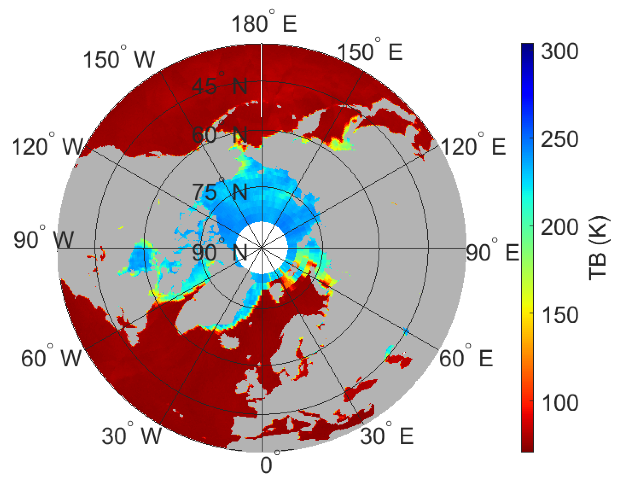
Figure 1. Example of daily averaged gridded brightness temperature (TB) over the Arctic on 1 January 2021.
Remotesensing 18 00265 g001
Figure 2. Flowchart of the synergistic optimization framework for L-band sea-ice concentration retrieval.
Remotesensing 18 00265 g002
Figure 3. (a) The daily TB scattered points in the seawater area (SIC = 0%), with 1 July 2020, as the start date. The color bar indicates the number of dispersion points. The darker the color, the denser the dots. (b) Probability density distribution of daily mean TB for regions with SIC = 0%. The red curve represents the fitted normal distribution with mean and standard deviation (SD (σ)) shown in the inset. The blue dot indicates the mode (most frequent value), while the red dot marks the mean of the normal distribution.
Remotesensing 18 00265 g003
Figure 4. (a) Bias of SIC retrieval under different SST thresholds compared with SSM/I. (b) RMSE of SIC retrieval under different SST thresholds compared with SSM/I. (c) Correlation coefficient (R) of SIC retrieval under different SST thresholds compared with SSM/I. Red and blue circles denote the SST values corresponding to the minimum and maximum of each metric, respectively.
Remotesensing 18 00265 g004
Figure 5. (a) The daily TB scattered points in fully ice-covered regions (SIC = 100%), with 1 July 2020, as the start date. The color bar indicates the number of dispersion points. The darker the color, the denser the dots. (b) Probability density distribution of daily mean TB for regions with SIC = 100%. The red curve represents the fitted normal distribution with mean and standard deviation (SD (σ)) shown in the inset. The blue dot indicates the mode (most frequent value), while the red dot marks the mean of the normal distribution.
Remotesensing 18 00265 g005
Figure 6. (a) Bias of SIC retrieval under different IST thresholds compared with SSM/I. (b) RMSE of SIC retrieval under different IST thresholds compared with SSM/I. (c) Correlation coefficient (R) of SIC retrieval under different IST thresholds compared with SSM/I. Red and blue circles denote the IST values corresponding to the minimum and maximum of each metric, respectively.
Remotesensing 18 00265 g006
Figure 7. Scatter plot of L-band SIC retrieved by Equation (7) versus SSM/I SIC, with scatter points color-coded by DAV. The black dashed line indicates the 1:1 line, and the solid black line represents the regression line.
Remotesensing 18 00265 g007
Figure 8. (a) Bias of SIC retrieval under different DAV thresholds compared with SSM/I. (b) RMSE of SIC retrieval under different DAV thresholds compared with SSM/I. (c) Correlation coefficient (R) of SIC retrieval under different DAV thresholds compared with SSM/I. Red and blue circles denote the DAV values corresponding to the minimum and maximum of each metric, respectively.
Remotesensing 18 00265 g008
Figure 9. The daily TB scattered points in the seawater regions ((a) SIC = 0%) and fully ice-covered regions ((c) SIC = 100%) after optimization in Section 3.2, with July 1, 2020, as the start date. The color bar indicates the number of dispersion points. The darker the color, the denser the dots. The probability density distribution of the daily mean TB for (b) SIC = 0% and (d) SIC = 100% after optimization in Section 3.2. The red curve represents the fitted normal distribution with mean and standard deviation (SD (σ)) shown in the inset. The blue dot indicates the mode (most frequent value), while the red dot marks the mean of the normal distribution.
Remotesensing 18 00265 g009
Figure 10. Comparison of L-band SIC retrieved without uncertainty mitigation (Equation (7)) with SSM/I SIC. The color bar represents the number of points scattered across the graph. The dashed line represents the 1:1 reference line, and the solid red line shows the linear regression fit (R = correlation coefficient, RMSE = root mean square error, y means SMAP SIC, and x means SSM/I SIC).
Remotesensing 18 00265 g010
Figure 11. L-band SIC retrieval after removing only the uncertainties of TBwater, compared with SSM/I SIC. The color bar represents the number of points scattered across the graph. The dashed line represents the 1:1 reference line, and the solid red line shows the linear regression fit (R = correlation coefficient, RMSE = root mean square error, y means SMAP SIC, and x means SSM/I SIC).
Remotesensing 18 00265 g011
Figure 12. L-band SIC retrieval after removing only the uncertainties of TBice, compared with SSM/I SIC. The color bar represents the number of points scattered across the graph. The dashed line represents the 1:1 reference line, and the solid red line shows the linear regression fit (R = correlation coefficient, RMSE = root mean square error, y means SMAP SIC, and x means SSM/I SIC).
Remotesensing 18 00265 g012
Figure 13. L-band SIC retrieval after removing only the uncertainties of DAV signals caused by sea Ice freeze-thaw, compared with SSM/I SIC. The color bar represents the number of points scattered across the graph. The dashed line represents the 1:1 reference line, and the solid red line shows the linear regression fit (R = correlation coefficient, RMSE = root mean square error, y means SMAP SIC, and x means SSM/I SIC).
Remotesensing 18 00265 g013
Figure 14. L-band SIC retrieval after removing only the uncertainties of incomplete land masking, compared with SSM/I SIC. The color bar represents the number of points scattered across the graph. The dashed line represents the 1:1 reference line, and the solid red line shows the linear regression fit (R = correlation coefficient, RMSE = root mean square error, y means SMAP SIC, and x means SSM/I SIC).
Remotesensing 18 00265 g014
Figure 15. (a) Remove only the pixels that are physically unsuitable for SIC retrieval based on the standard SIC definition. (b) L-band SIC retrieval after removing four uncertainties of TBwater, TBice, DAV, and incomplete land masking, compared with SSM/I SIC. The color bar represents the number of points scattered across the graph. The dashed line represents the 1:1 reference line, and the solid red line shows the linear regression fit (R = correlation coefficient, RMSE = root mean square error, y means SMAP SIC, and x means SSM/I SIC).
Remotesensing 18 00265 g015
Figure 16. Comparison of algorithm results with SSM/I SIC data using a 1:1 scatter plot during stepwise optimization.
Remotesensing 18 00265 g016
Figure 17. (al) Illustrate the robustness analysis of the algorithm over 12 months, from July 2020 to June 2021. The horizontal axis represents each month’s SSM/I SIC. The vertical axis shows the retrieved SIC. The color bar represents the number of points scattered across the graph. The dashed line represents the 1:1 reference line, and the solid red line shows the linear regression fit (R = correlation coefficient, RMSE = root mean square error, y means SMAP SIC, and x means SSM/I SIC).
Remotesensing 18 00265 g017
Figure 18. (a) Interannual Variation of L-band retrieved SIC Algorithm (15% SIC contour lines); (b) Interannual Variation of SSM/I SIC (5% SIC contour lines); (c) Daily difference of minimum SIC extent (derived by L-band SIC): 11 September 2020; (d) Daily difference of maximum SIC (derived by L-band SIC): 7 March 2021.
Remotesensing 18 00265 g018
Figure 19. (a) Scatter plot comparing SIC retrieved by the new L-band algorithm versus ship-based observations (from 1 July 2020, to 30 June 2021). The black dashed line represents the 1:1 reference line, and the green solid line shows the linear regression fit (R = correlation coefficient, RMSE = root mean square error, MAE = mean absolute error); (b) Same as (a), but for SSM/I SIC versus ship-based observations. (c) Distribution of differences between the new L-band algorithm’s SIC and the ship-based SIC. (d) Distribution of differences between SSM/I SIC and ship-based SIC.
Remotesensing 18 00265 g019
Figure 20. (a) Scatter plot comparing SIC retrieved by the new L-band algorithm versus SAR-based observations (from 1 July 2020, to 30 June 2021). The black dashed line represents the 1:1 reference line, and the green solid line shows the linear regression fit (R = correlation coefficient, RMSE = root mean square error, MAE = mean absolute error); (b) Same as (a), but for SSM/I SIC versus SAR observations. (c) Distribution of differences between the new L-band algorithm’s SIC and SAR-based SIC. (d) Distribution of differences between SSM/I SIC and SAR SIC.
Remotesensing 18 00265 g020
Figure 21. A time series of the L-band (1.41 GHz) DAV signal at a representative location.
Remotesensing 18 00265 g021
Figure 22. Daily L-band SIC Results Derived from Ascending and Descending Passes Highlighting DAV Effects.
Remotesensing 18 00265 g022
Table 1. Summary of datasets used in this study.
DatasetProductSpatial ResolutionPrimary Role in This Study
Core input
L-band TB
(Twice a day for high-latitude areas)
SMAP SPL3FTP (Version 3)36 kmPrimary input for SIC retrieval and DAV calculation.
Constraint & Endmember definition
ERA5 SIC, SST, IST (Hourly)ERA5 (ECMWF)0.25°Define pure water (SIC = 0%) and pure ice (SIC = 100%) endmember regions; quantify impacts of warm water (SST) and extremely low temperature conditions of ice (0–7 cm layer ice temperature).
Reference for optimization and evaluation
SSM/I SIC (Daily)SSM/I-SSMIS (NASA Team, Version 2)25 kmPrimary reference for algorithm threshold determination, optimization, and performance evaluation.
Independent validation
Ship-based SIC(Hourly)ICEWatch/ASSIST ProgramPoint observationIn situ validation source.
SAR SIC (Daily)Arctic Ocean—High Resolution Sea Ice Information L41 kmHigh-resolution reference for validation.
Table 2. Evaluation of endmembers without considering uncertainties. The bolded column indicates the Group with the best performance for each criterion.
GroupΔμ (K)RSD (Seawater)RSD (Sea Ice)CNR
TBH155.9810.095.7610.00
PD24.133.5124.116.51
PR0.306.0633.3313.42
Table 3. Evaluation of endmembers considering uncertainties. The bolded column indicates the Group with the best performance for each criterion.
GroupΔμ (K)RSD (Seawater)RSD (Sea Ice)CNR
TBH1601.622.7823.94
PD24.771.8620.248.54
PR0.312.9433.3321.93
Disclaimer/Publisher’s Note: The statements, opinions and data contained in all publications are solely those of the individual author(s) and contributor(s) and not of MDPI and/or the editor(s). MDPI and/or the editor(s) disclaim responsibility for any injury to people or property resulting from any ideas, methods, instructions or products referred to in the content.