Three-Dimensional Radar Echo Extrapolation Using a Physics-Constrained Deep Learning Model

Highlights

What are the main findings?

• DIFF-3DRformer, a novel deep learning framework for 3D radar echo extrapolation, integrates a mesoscale evolution network with 3D advection equation neural operators and a 3D continuity equation-informed loss function, along with a convective-scale denoising generative network.
• When evaluated on severe convective storm events in Jiangsu, China, DIFF-3DRformer achieves a 44.8% improvement in overall performance score over NowcastNet for reflectivity thresholds ≥ 35 dBZ.

What are the implications of the main finding?

• The use of 19 vertical levels of radar data significantly enhances the prediction of convective echo morphology and intensity, outperforming methods using only composite reflectivity.
• The incorporation of physical constraints improves the spatial accuracy and structural consistency of forecasted radar echoes, offering a robust solution for 3D convective storm characterization.

Abstract

Accurate nowcasting of severe convective storms is crucial for disaster mitigation, yet storm complexity challenges conventional deep learning models. Existing methods often use single-level radar data and lack physical constraints, limiting skill in predicting small-scale convective systems. To address this, we propose DIFF-3DRformer, a novel deep learning framework for 3D radar echo extrapolation. This model unifies a mesoscale evolution network, embedded with 3D advection equation neural operators and a 3D continuity equation-informed loss function, and a convective-scale denoising generative network based on a diffusion model, within an end-to-end architecture optimized for prediction accuracy. Evaluated on severe storm events over Jiangsu, China, DIFF-3DRformer demonstrates robust predictive skill across various convective scales. It outperforms NowcastNet, improving the comprehensive score by 44.8% for reflectivity thresholds ≥35 dBZ. Utilizing 19 vertical levels of radar data as input significantly enhances the morphology and intensity prediction of convective echoes, boosting performance by 4.63% compared to using only composite reflectivity. Furthermore, the incorporation of physical constraints refines the forecasted echo structure and spatial placement, yielding additional improvements. DIFF-3DRformer provides accurate short-term evolution forecasts of convective systems, offering a promising solution for developing nowcasting methods that directly characterize the 3D structure of convective storms.

1. Introduction

Severe convective weather is a meteorological phenomenon generated by intense vertical upward motion of air. The hazardous weather events induced thereby, such as thunderstorm gales, short-duration heavy rainfall, and hail, pose a significant threat to human life and property, agricultural production, urban infrastructure, and the ecological environment. Consequently, accurate, timely, and high-resolution nowcasting is critical for early warning systems and risk mitigation of meteorological disasters.

Due to constraints in computational resources and uncertainties in initial and boundary conditions, numerical weather prediction (NWP) remains challenged in providing accurate short-term nowcasts for the 0–2 h range, particularly at the 1 km scale and with update frequencies within 10 min [1]. Furthermore, convective weather systems are characterized by rapid development and dissipation, as well as small spatial scales, making them difficult to capture using conventional observations and forecasting techniques with relatively coarse temporal and spatial resolution. Weather radar, by contrast, offers high spatiotemporal resolution observations of the atmosphere. Therefore, extrapolation-based nowcasting using radar echo sequences presents a viable approach for predicting convective initiation and evolution [2].

Current approaches for nowcasting severe convective storms primarily rely on radar observations at specific altitude levels or composite reflectivity sequences. Traditional nowcasting methods, such as cross correlation, optical flow and tracking method [3,4,5,6], have been widely used but often lack sufficient nonlinear mapping capability. This limitation hinders their ability to accurately capture the long-term evolutionary trends of intense convection [7]. In recent years, deep learning techniques have shown promising potential in nowcasting of convective storms [8,9,10,11,12]. Compared to traditional techniques, deep learning models have demonstrated a capacity for predicting the initiation, development, and dissipation of convective storms [13]. For instance, Shi et al. [14] proposed Convolutional Long Short-Term Memory (ConvLSTM), which integrates convolutional layers with Long Short-Term Memory networks, for precipitation nowcasting. To address issues of insufficient input information and suboptimal model structure, the Fusion and Reassignment Network (FURENet) was designed to extract information from dual-polarization radar variables and improve storm forecasting [15]. However, a common drawback among these deep learning models is the gradual blurring of forecast details at longer lead times. To mitigate the smoothing effect often seen in deep learning forecasts, the Deep Generative Model of Rainfall (DGMR) was developed, utilizing generative networks to produce realistic rainfall forecasts up to 90 min ahead [16]. More recently, the NowcastNet model, which combines physical evolution mechanisms with generative adversarial networks, was shown to enhance the forecasting capability for extreme precipitation events within 0–3 h [17]. Despite these advances, most existing studies are based on single-level radar reflectivity fields and lack a detailed characterization of the vertical structure of convective storms. The development of convective systems, however, exhibits distinct vertical structural characteristics. The persistence of intense radar echoes at upper levels often signals potential severe weather hazards. Furthermore, the spatial distribution of heavy precipitation and its peak intensity are closely related to the storm’s vertical architecture. Consequently, relying solely on two-dimensional radar reflectivity from a single altitude level fails to capture the interdependencies between different heights, thus providing an incomplete representation of the convective system’s structure [18,19]. Zhang et al. [20] applied multichannel 3D convolutional neural networks(3DCNNs) to 3D radar echo extrapolation but did not characterize the performance differences between using 3D versus 2D radar echo data as input. Subsequent approaches based on 3D convolutional recurrent neural networks [21,22] have been proposed for 3D radar echo extrapolation, however, these methods still tend to underestimate convective storm intensity.

To address these challenges, this study proposes a deep learning framework incorporating physical constraints for three-dimensional (3D) radar echo extrapolation. The framework designs a 3D radar echo feature encoder based on the Dual Attention Vision Transformer (DaViT) [23], which alternately applies spatial window attention and channel group attention to capture the motion characteristics and long short-term dependencies of 3D radar echoes. A reflectivity predictor and a 3D velocity field predictor are constructed based on 3D Convolutional Neural Networks (3D-CNNs) to simultaneously forecast the evolution of 3D reflectivity and the 3D velocity field. A custom advection neural operator is then employed, which utilizes the predicted 3D velocity field to advect and update the reflectivity prediction. Furthermore, the 3D continuity equation is integrated into the model by adding a divergence loss term to the standard Mean Squared Error (MSE) loss function, thereby constraining the predicted 3D velocity field to satisfy mass conservation. To further improve the forecasting skill for convective-scale echoes, a probabilistic diffusion model [24] is incorporated to simulate the relatively stochastic initiation and dissipation processes of convective-scale echoes.

The paper is structured as follows. Section 2 presents the dataset and experimental design. Section 3 presents experimental results, including results on three representative cases and quantitative performance evaluation. Section 4 discuss and analysis this study. Section 5 concludes the research and and explores potential directions for future research.

2. Materials and Methods

2.1. Data

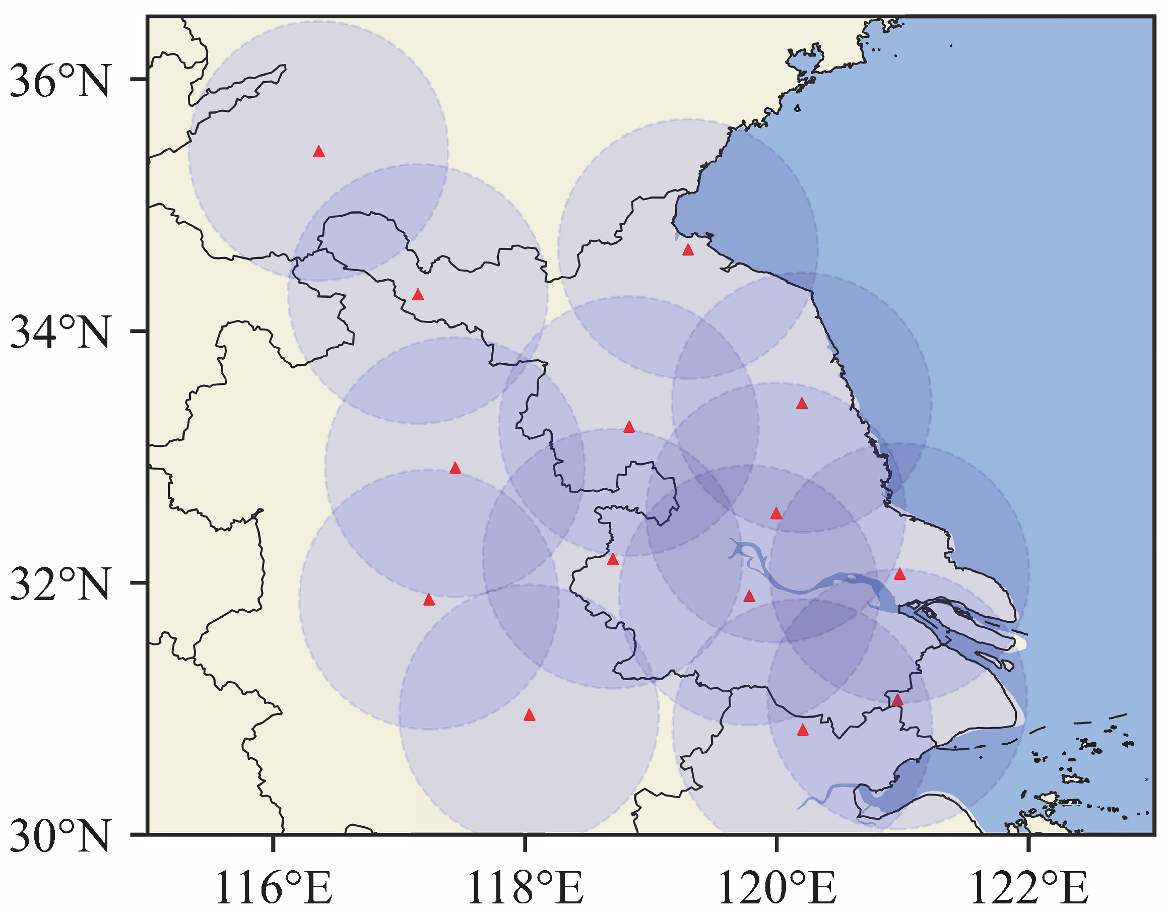
As shown in Figure 1, this study focuses on a target region that covers most of Jiangsu Province and its upstream areas in Anhui Province, China. A radar mosaic dataset was constructed using S-band dual-polarization weather radar data set from multiple radars in Jiangsu Province collected during the rainy seasons (April–September) from 2020 to 2025. The initial data underwent comprehensive quality control and mosaic processing. First, a fuzzy logic classifier [25] was employed to remove non-meteorological echoes from the multi-elevation base reflectivity observations of each radar. Low-level observations are indeed critical for representing convective initiation and evolution, therefore, we retain reflectivity from the near-surface layer up to 3 km in our preprocessing. In the Jiangsu region, where the terrain is predominantly plains, terrain shielding from the operational S-Band Dual-Polarization Radar is generally limited. Nevertheless, isolated low-elevation beam blockage can occur at a few local sites. To mitigate this, we employ a 13-radar mosaic network combined with data interpolation to reduce the impact of such gaps on both training and evaluation. Subsequently, the quality-controlled base reflectivity data were interpolated onto different constant-altitude planes (0–9 km, with a vertical resolution of 500 m) within a Cartesian coordinate system and then mosaicked. This process yielded a three-dimensional, multi-altitude gridded reflectivity mosaic product with a high spatial resolution of $0.{01}^{\circ }$ and a temporal resolution of 6 min. For the present analysis, we utilize the complete set of all 19 available constant-altitude planes from this mosaic product. We partitioned the data from April–September of each year during 2020–2024 into a training set and a validation set at an 8:2 ratio and used the April–September 2025 data as the test set.

2.2. Experimental Design

The radar reflectivity factor measured by the weather radar is directly related to the concentration and size of precipitation particles. Consequently, the current radar reflectivity map can effectively reveal the spatial distribution and intensity of precipitation within a specific area. A time series of consecutive radar reflectivity observations captures the evolution, including the initiation, development, and dissipation, of cloud systems over a region, making radar echo extrapolation a critical technique for short-term forecasting of severe convective weather. Radar echo extrapolation involves predicting future radar echo images based on a sequence of historical observations. Specifically, using a sequence of radar reflectivity data from the past J time steps to predict the subsequent K time steps can be formulated as a conditional probability problem, leading to the probability expression given in Equation (1):

$${\tilde{\chi }}_{t+1},\dots ,{\tilde{\chi }}_{t+K}=\underset{{\chi }_{t+1},\dots ,{\chi }_{t+K}}{argmax}p({\chi }_{t+1},\dots ,{\chi }_{t+K}|{\widehat{\chi }}_{t-J+1},{\widehat{\chi }}_{t-J+2},\dots ,{\widehat{\chi }}_t)$$

(1)

In this study, a spatiotemporal deep learning model is employed to address the aforementioned issue. By stacking the reflectivity data from different levels at the same time step to form a channel dimension, the three-dimensional radar echo nowcasting problem can be formally defined by the following Equation (2).

$$\begin{array}{cc}\hfill {\tilde{\chi }}_{t+1},\dots ,{\tilde{\chi }}_{t+K}& =\mathcal{M}\left({\widehat{\chi }}_{t-J+1},{\widehat{\chi }}_{t-J+2},\dots ,{\widehat{\chi }}_t\right),\hfill \\ \hfill \tilde{\chi },\widehat{\chi }& \in {\mathbb{R}}^{C\times H\times W}(C=19)\hfill \end{array}$$

(2)

where $\mathcal{M}$ is the nowcasting model, while J and K are the time steps of input and output. In this study, the model uses the past 30 min radar echo sequence to predict the subsequent 2 h sequence. Given that the radar observations are sampled at 6 min intervals, so J is set to 5 and K to 20. As such, a single sample contains radar data of 25 time steps in total.

As shown in

Table 1. The details of three sets of controlled experiments.

Controlled Experiment Scheme	Scheme Description	Function
Zh1_PredRNNV2	Use single-level radar echo data (take the maximum value of 19 height levels) and the PredRNNV2 model	Scheme 1: Evaluate the performance of the DIFF-3DRformer model against other nowcasting methods
Zh1_NowcastNet	Use single-level radar echo data (take the maximum value of 19 height levels) and the NowcastNet model
Zh1_DIFF-3DRformer	Use single-level radar echo data (take the maximum value of 19 height levels) and the DIFF-3DRformer model
Zh1_DIFF-3DRformer	Use single-level radar echo data (take the maximum value of 19 height levels)	Scheme 2: Examine the impact of adding more radar echo data levels on the model
Zh10_DIFF-3DRformer	Use 10-level radar echo data with 0–9 km (1 km interval)
Zh19_DIFF-3DRformer	Use 19-level radar echo data with 0–9 km (500 m interval)
Zh19_Transformer	Use 19-level radar echo data with 0–9 km (500 m interval) and the Spatio-Temporal Transformer model without physical constraints	Scheme 3: Verify the impact of adding physical-constraint neural operators and convective-scale diffusion models on model performance
Zh19_3DRformer	Use 19-level radar echo data with 0–9 km (500 m interval) and the 3DRformer
Zh19_DIFF-3DRformer	Use 19-level radar echo data with 0–9 km (500 m interval) and the DIFF-3DRformer

, We conducted three sets of controlled experiments. The first set of experiments established baseline performance using two models: Zh1_PredRNNV2 [8] and Zh1_NowcastNet [17]. To ensure a consistent comparison, as the original NowcastNet utilizes only single-level radar echo data, we compared these baselines against the Zh1_DIFF-3DRformer scheme, which is also trained on single-level composite reflectivity(CR) data. This comparison aims to evaluate the performance of DIFF-3DRformer against other benchmark models. The second set of experiments implemented three configurations of the DIFF-3DRformer architecture: Zh1_DIFF-3DRformer, Zh10_DIFF-3DRformer, and Zh19_DIFF-3DRformer. These were designed to investigate the impact of incorporating more vertical levels of reflectivity data. The Zh1_DIFF-3DRformer model uses only the maximum value in the vertical column from the 19 available altitude levels (i.e., a single level) as input. The Zh10_DIFF-3DRformer uses 10 specific levels (0, 1, 2, 3, 4, 5, 6, 7, 8, and 9 km), while the Zh19_DIFF-3DRformer employs all 19 levels. A third set of ablation experiments was conducted to isolate the contributions of key architectural components. This involved comparing three schemes: Zh19_Transformer, Zh19_3DRformer, and Zh19_DIFF-3DRformer. The Zh19_Transformer experiment used the same input variables as Zh19_DIFF-3DRformer but incorporated neither the physics-constrained neural operator nor the diffusion model. The Zh19_3DRformer experiment used the same inputs and the physics-constrained neural operator but did not include the diffusion model.

2.3. DIFF-3DRformer

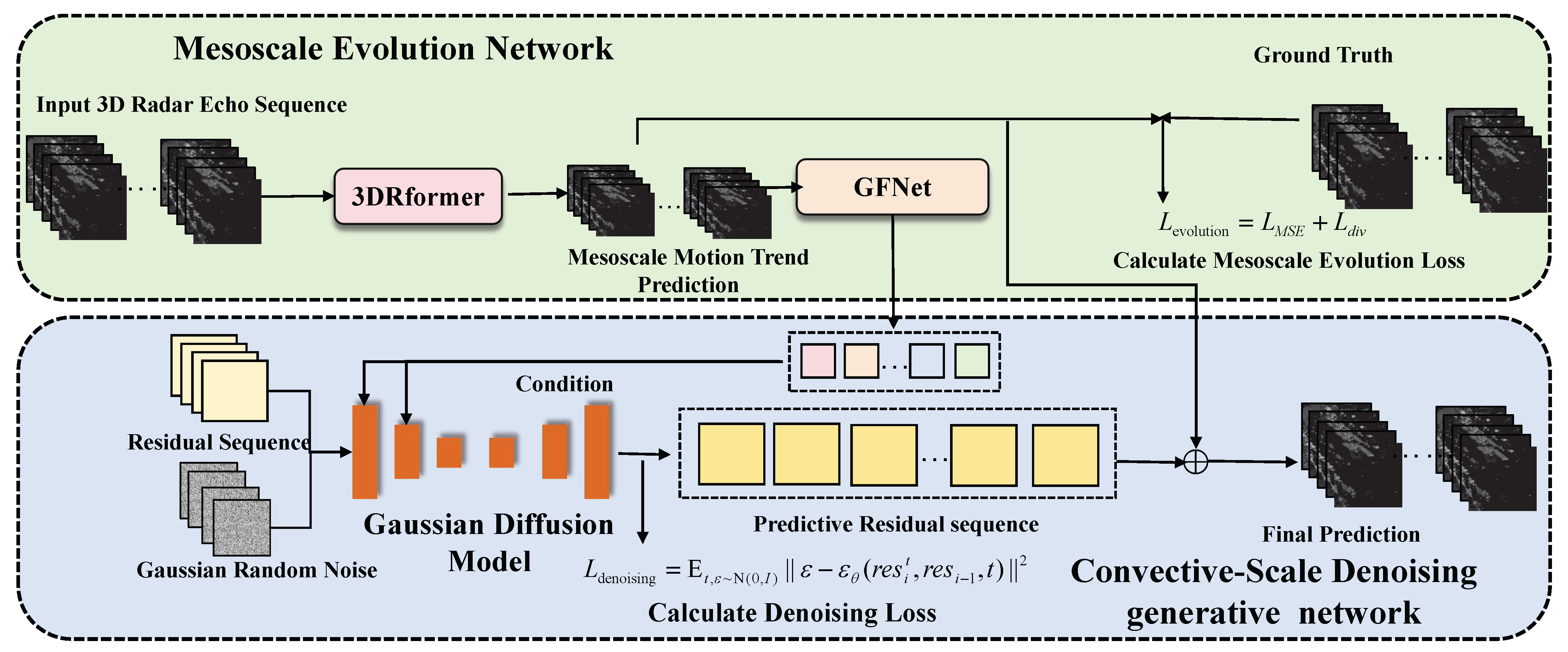
Based on our previous work [26], we have further improved the model for the three-dimensional (3D) radar echo extrapolation problem. As illustrated in Figure 2, the overall architecture comprises a mesoscale evolution network and a convective-scale denoising generative network, dedicated to modeling the mesoscale echo motion trends and the convective-scale initiation and dissipation processes, respectively. A key enhancement involves the mesoscale evolution network, for which we propose a 3D Radar Transformer (3DRformer), a neural operator based on the 3D advection equation, to model the spatiotemporal evolution of echo features. This component incorporates dedicated decoders for the motion velocity field and the reflectivity factor, predicting the velocity field and reflectivity factor separately. A custom 3D differentiable physical advection operator is introduced to explicitly embed principles of fluid dynamics. Furthermore, the divergence of the velocity field is incorporated as a regularization term in the loss function, constraining the velocity field to satisfy the 3D continuity equation. The architecture of the convective-scale denoising generative network remains identical to that in the original study.

2.4. 3DRformer

To better simulate the motion trends of radar echoes, inspired by the NowcastNet framework, we integrate physical evolution schemes with deep learning models within a unified neural network architecture. As shown in Figure 3, by extending the two-dimensional radar echo inputs into three-dimensional data, we design 3DRformer—a spatiotemporal echo evolution model based on a 3D advection-equation-informed neural operator.

The overall framework can be summarized as follows: a historical 3D radar echo sequence is input into a powerful spatio-temporal feature extractor (encoder) to learn its evolutionary patterns. The extracted features are then fed into two separate decoders: one predicts the 3D motion velocity field driving echo movement, and the other predicts a residual term representing changes in echo intensity. The predicted velocity field is subsequently used as a physical constraint to drive an explicit 3D physical advection operator. The final forecast is obtained by summing the advected result and the residual prediction.

The input consists of a sequence of three-dimensional radar reflectivity fields from consecutive time steps. The Spatio-Temporal Transformer encoder, which adopts a structure similar to DaViT. is tasked with constructing a latent feature representation that comprehensively captures the spatio-temporal dependencies within the echo sequence. The encoded latent features are directed into two distinct decoders—a velocity field decoder and a reflectivity factor decoder. Although these decoders share a similar 3D convolutional architecture, they serve different purposes. The velocity field decoder regresses the average motion field driving radar echo movement over the future time steps, while the reflectivity factor decoder predicts the residual term for the future reflectivity sequence, accounting for intensity changes. Specifically, we employ a motion decoder to directly predict the instantaneous velocity field $v\_t$ from a sequence of past radar echo observations and an intensity decoder to predict the intensity residual $s\_t$. A differentiable evolution operator then advances the state by first advecting with $v\_t$ and subsequently adding the residual $s\_t$, yielding a physically consistent evolution field. The entire framework is constrained by the continuity equation and optimized via an end-to-end loss, ensuring that predictions adhere to advective conservation while capturing nonlinear evolution. Then the predicted intensity field and motion field are then integrated through a 3D physical advection operator. This operator advects the last observed radar frame using the motion field and adds the residual intensity field to generate the final prediction. The 3D physical advection operator is a non-learnable, deterministic numerical process. It takes the previously predicted echo field as the advected field and the corresponding motion field predicted by the velocity decoder to solve the 3D advection equation:

$${\displaystyle \frac{\partial \varphi }{\partial t}}+\overrightarrow{V}·\nabla \varphi =0$$

(3)

where $\varphi (x,y,z,t)$ denotes the three-dimensional radar echo scalar field, ${\displaystyle \frac{\partial \varphi }{\partial t}}$ represents the local rate of change in $\varphi$, $\overrightarrow{V}·\nabla \varphi =u{\displaystyle \frac{\partial \varphi }{\partial x}}+v{\displaystyle \frac{\partial \varphi }{\partial y}}+w{\displaystyle \frac{\partial \varphi }{\partial z}}$ stands for the advection term, $(u,v,w)$ is the velocity vector, and ∇ refers to the gradient operator. By integrating the physical consistency of operators in predicting large-scale echo motions with the ability of neural networks to capture nonlinear local variations, this approach more faithfully captures the spatiotemporal evolution of echo characteristics. In the 3DRformer framework, the velocity field in the advection equation should correspond to the echo displacement field, whereas radial velocity measured by radar is the projection along the beam direction and is neither purely nor directly equivalent to the velocity required for advection, and this study focuses on simulating echo motion. Furthermore, 3DRformer implements the advection process as a differentiable neural evolution operator, enabling gradient backpropagation to directly minimize forecast errors. Therefore, radial velocity observations were not considered as additional input information.

2.5. Formulating the Loss Function Using the 3D Continuity Equation

In the 3DRformer architecture described in Section 3.2, the velocity decoder relies on deep learning components to directly regress the 3D motion field of radar echoes. A key limitation is that this process lacks explicit physical constraints, as true observations of wind or echo motion fields are unavailable, which may lead to physically unreliable velocity predictions. To address this, we introduce a regularization term based on the 3D continuity equation into the model. Specifically, by minimizing the divergence of the velocity field as an additional training objective, the network is forced to generate a velocity field that approximately satisfies the mass conservation law for a source-free flow. This enhancement significantly improves the physical plausibility of the predicted motion field. Consequently, when coupled with a physical advection operator, it leads to radar echo predictions that are not only statistically accurate but also more consistent with dynamical principles.

For many atmospheric motions, particularly at the spatiotemporal scales central to nowcasting, the effect of air density changes is relatively small. The continuity equation can thus be approximated by that for an incompressible fluid, which simplifies to a divergence-free condition on the velocity field [27]:

$$\nabla ·\overrightarrow{V}={\displaystyle \frac{\partial u}{\partial x}}+{\displaystyle \frac{\partial v}{\partial y}}+{\displaystyle \frac{\partial w}{\partial z}}=0$$

(4)

In numerical simulations, the central difference method is employed to approximate the velocity field at each grid point:

$${\left(\nabla ·\overrightarrow{V}\right)}_{i,j,k}\approx {\displaystyle \frac{u_{i+1,j,k}-u_{i-1,j,k}}{2\Delta x}}+{\displaystyle \frac{v_{i,j+1,k}-v_{i,j-1,k}}{2\Delta y}}+{\displaystyle \frac{w_{i,j,k+1}-w_{i,j,k-1}}{2\Delta z}}$$

(5)

In the Equation (5), $\Delta x$, $\Delta y$ and $\Delta z$ represent the grid spacing. Based on the given calculation formula, the divergence loss can be defined as the sum (or average) of the squared divergence across all grid points in the predicted velocity field. This formulation aims to minimize the deviation of the divergence from its physically ideal value of zero:

$$L_{\mathrm{div}}={\displaystyle \frac{1}{N}}\sum _{\mathsf{\Omega }}{|\nabla ·\overrightarrow{V}|}^2$$

(6)

where N represents the total number of grid points. The $L_{\mathrm{div}}$ acting as a physical regularization, is applied directly to the output of the velocity field decoder. This direct application constrains the parameter updates, steering the model toward generating a velocity field that is more consistent with physical laws. Furthermore, to minimize the discrepancy between the predicted and actual echo intensity fields, we adopt the root mean square error (MSE) as the loss function for the data fitting procedure:

$$L_{\mathrm{MSE}}={\displaystyle \frac{1}{N}}\sum _{i=1}^N{(y_i-{\widehat{y}}_i)}^2$$

(7)

where N represents the total number of grid points. $y_i$ denotes the observed radar reflectivity factor field, and ${\widehat{y}}_i$ represents the predicted field. By combining these two components, the total loss function of the mesoscale evolution network is formulated as follows:

$$L_{\mathrm{evolution}}=L_{\mathrm{MSE}}+\lambda L_{\mathrm{div}}$$

(8)

where $\lambda$ is a hyperparameter that balances the magnitude between the two loss functions.

2.6. Evaluation Metrics

We employ the novel comprehensive score (Score) proposed by ZENG et al. [28] to evaluate the model’s forecasting performance. This metric synthetically incorporates three aspects: forecast skill, forecast balance, and forecast authenticity. The calculation formula for the Score is as follows:

$$\mathrm{Score}=\mathrm{TS}·exp{[-|1-\mathrm{Bias}\left|\right]}^{0.2}·exp{\left(-{\displaystyle \frac{\mathrm{FID}}{100}}\right)}^{0.2}$$

(9)

This metric integrates the Threat Score (TS), Bias score, and Fréchet Inception Distance (FID) score. The TS, commonly used in operational forecasting as a measure of forecast skill, serves as the baseline score in the equation. The method for calculating TS is shown as follows:

$$\mathrm{TS}={\displaystyle \frac{\mathrm{TP}}{\mathrm{TP}+\mathrm{FN}+\mathrm{FP}}}$$

(10)

where TP (True Positives) are correctly predicted events, FN (False Negatives) are missed events, and FP (False Positives) are incorrectly predicted events.

The Bias score assesses the “balance” of the forecast results, with values closer to 1 indicating better performance. The Bias is computed as follows:

$$\mathrm{Bias}={\displaystyle \frac{\mathrm{TP}+\mathrm{FP}}{\mathrm{TP}+\mathrm{FN}}}$$

(11)

The FID measures the sharpness of the forecast, where a higher FID value corresponds to lower forecast precision. The FID is defined as:

$$\mathrm{FID}=\parallel {\mu }_r-{\mu }_g{\parallel }^2+\mathrm{Tr}\left({\mathsf{\Sigma }}_r+{\mathsf{\Sigma }}_g-2\sqrt{{\mathsf{\Sigma }}_r{\mathsf{\Sigma }}_g}\right)$$

(12)

here ${\mu }_r$ represents the mean vector of the multivariate Gaussian distribution that models the feature embeddings derived from the Inception-v3 network of the ground-truth. ${\mu }_g$ denotes the mean vector of the multivariate Gaussian distribution that models the generated data feature embeddings from the same Inception-v3 network. ${\mathsf{\Sigma }}_r$ and ${\mathsf{\Sigma }}_g$ denotes the covariance matrices of real and generated image distributions.

To quantitatively evaluate the reflectivity intensity error between the observed and predicted radar echo fields, the Root Mean Square Error (RMSE) is employed, which is defined as:

$$\mathrm{RMSE}=\sqrt{{\displaystyle \frac{1}{n}}\sum _{i=1}^n{(y_i-{\widehat{y}}_i)}^2}$$

(13)

where n is the total number of grid points, $y_i$ denotes the observation field and ${\widehat{y}}_i$ denotes the forecast field.

3. Results

3.1. Representative Cases

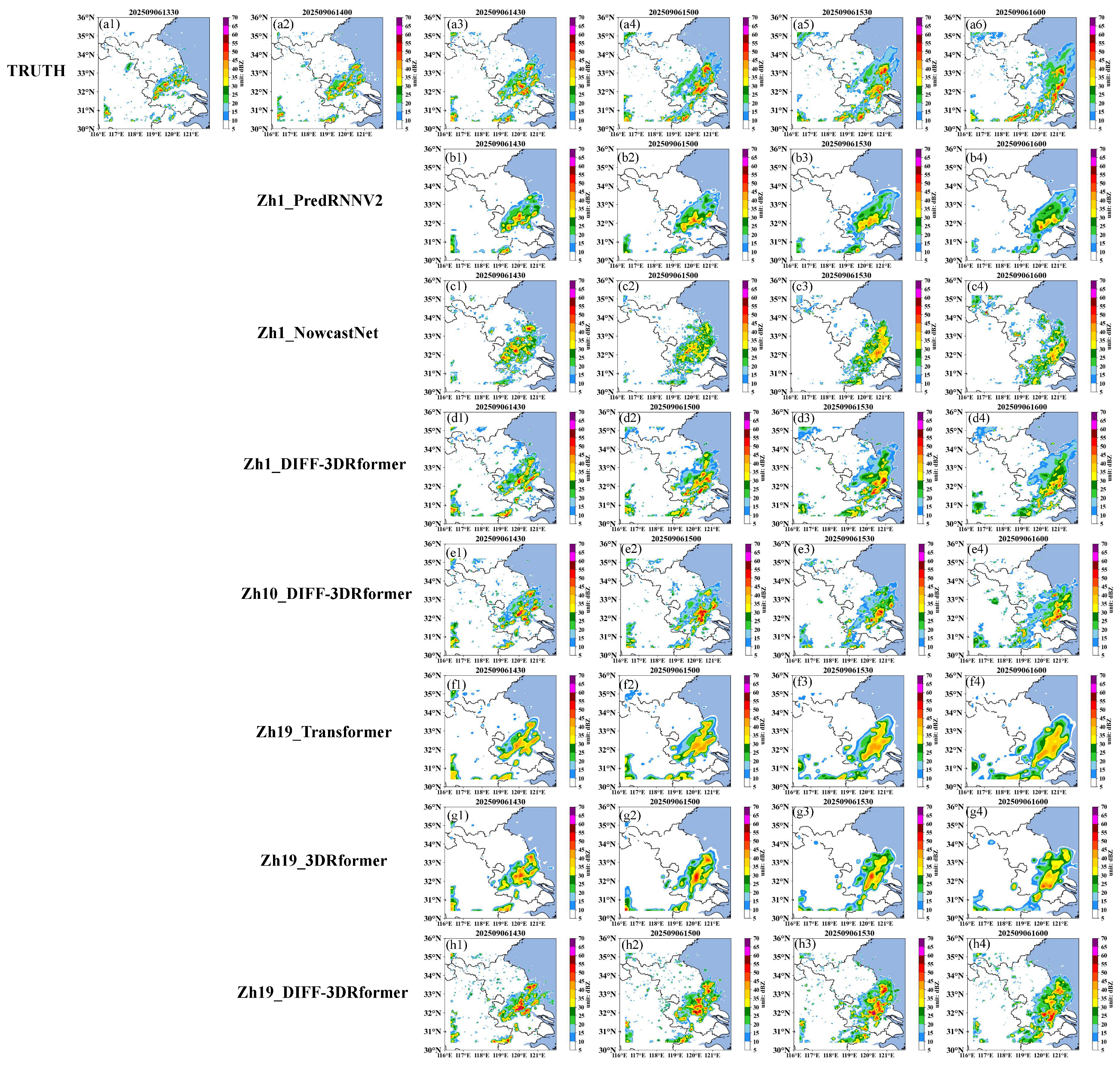
Figure 4 presents a convective organization case observed over Jiangsu Province from 14:06 to 16:00 Beijing Time on 6 September 2025. The figure compares real observations (a1–a6) with outputs from three sets of controlled experimental models. For models capable of predicting multi-layer radar echoes, the maximum vertical column reflectivity is displayed. Radar images are shown at 30 min intervals for clarity. Observations reveal that a new convective storm initiated south of Taizhou between 14:00 and 14:30, which subsequently merged with pre-existing storms to the west and organized into a linear convective system along the coastal area. For the first set of controlled experiments, The PredRNNV2 experiment failed to capture this convective initiation. NowcastNet only predicted the initiation around 15:30 (c3), which lagged considerably behind observations. In contrast, DIFF-3DRformer accurately and timely detected the convective initiation and reasonably predicted its organization into a linear system, although the predicted system intensity at 16:00 (d4) was weaker than observed. This case demonstrates that the proposed DIFF-3DRformer outperforms both PredRNNV2 and NowcastNet in forecasting convective initiation. For the second set of controlled experiments, Zh1_DIFF-3DRformer, Zh10_DIFF-3DRformer, and Zh19_DIFF-3DRformer successfully captured the development of this convective initiation. However, Zh1_DIFF-3DRformer underestimated the linear convective system over coastal southeastern China at 16:00 (d4), whereas Zh10_DIFF-3DRformer substantially mitigated this underestimation (e4). Zh19_DIFF-3DRformer yielded intensity and precipitation-region forecasts closest to the observations (h4). These results indicate that increasing the number of radar echo input levels can effectively alleviate the intensity bias in forecasts of strong convective systems. For the third set, the Zh19_Transformer scheme exhibited progressively degraded morphology and displacement of the strong convective system with lead time (f1–f4). Incorporating additional physics constraints in Zh19_3DRformer improved the representation of strong echo morphology and intensity in the first hour (g1–g2) but still underestimated peak reflectivity by the second hour (g3–g4). Further augmenting the model with a diffusion model in Zh19_DIFF-3DRformer maintained accurate intensity and structural depiction of the convective system at later lead times. Overall, physics-constrained training enhances early-period convective echo forecasts, but performance still degrades with lead time; the addition of a diffusion model effectively extends the useful forecast lead time for strong convection.

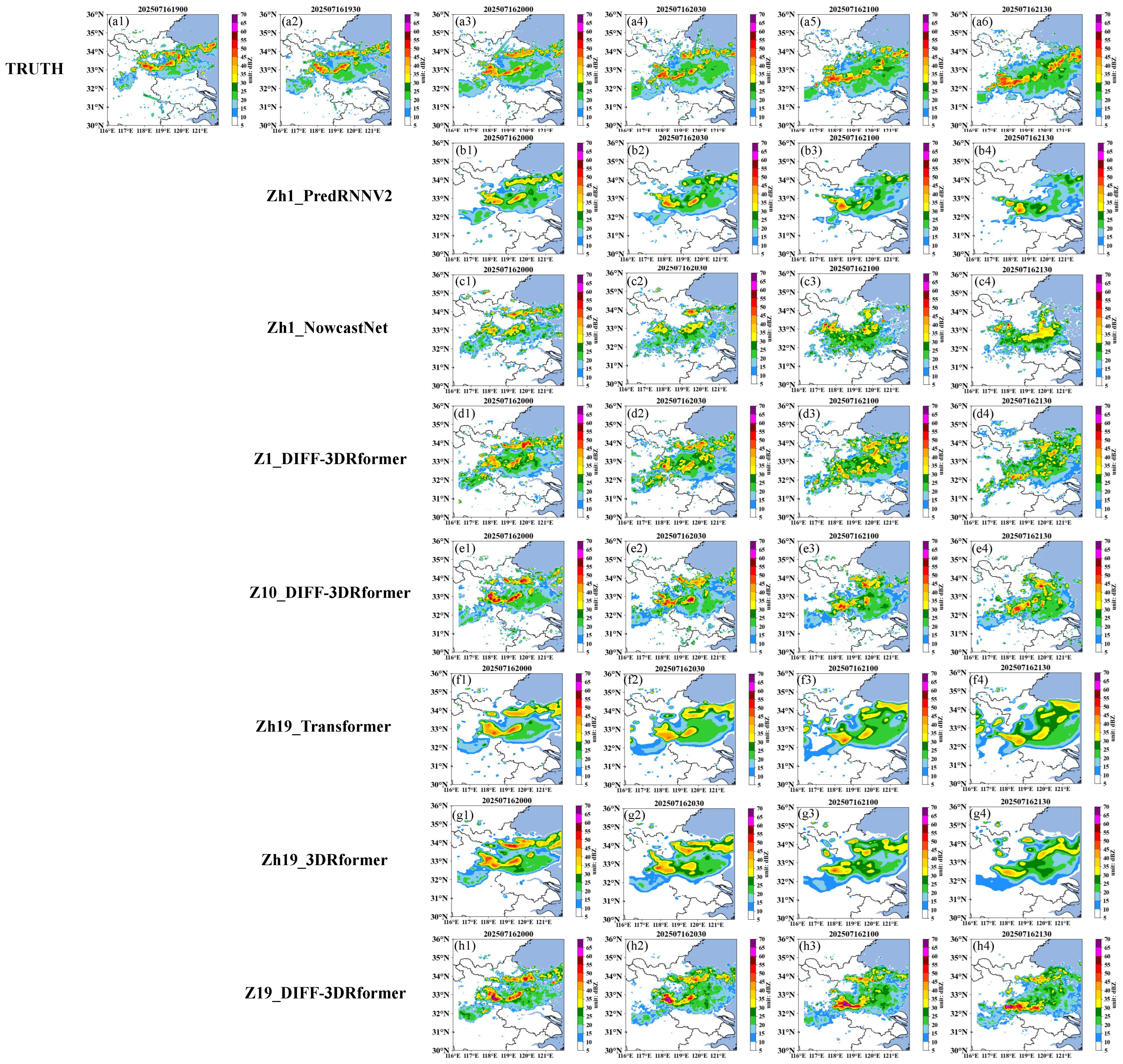
Figure 5 presents a case study of a large-scale squall line over Jiangsu, China, from 19:36 to 21:30 Beijing Time on 16 July 2025. The figure compares the ground-truth observations (a1–a6) with outputs from three sets of controlled experimental models. Observations reveal that the convective system propagated south-southeastward, progressively intensifying and becoming more organized, eventually affecting the Nanjing area. The Zh1_PredRNNV2 model exhibits limited skill in squall-line forecasting, with the system’s intensity consistently underestimated and the bias becoming more pronounced in the later forecast hours (b3–b4). Although Zh1_NowcastNet captures the squall line’s location and morphology at 21:30 (c4), its predicted intensity is markedly weaker than that of the observations. Z1_DIFF-3DRformer better predicts the squall line’s location in the later stages, yet the intensity remains underestimated. Overall, DIFF-3DRformer achieves the best performance among the three models for this case. The Zh1_DIFF-3DRformer experiment, which utilized only a single echo level failed to capture the intensity and spatial extent of the strong convection, producing a disorganized and significantly weakened squall line structure. In contrast, the Zh10_DIFF-3DRformer experiment, incorporating 10 echo levels, effectively captured the overall location and organization of the convective system, though it still underestimated the intensity and poorly delineated storm boundaries. The Zh19_DIFF-3DRformer experiment, using 19 input levels, successfully reproduced the linear convective organization process. By 21:30 (h4), it accurately predicted the intensity and position of the line-shaped convection north of Nanjing, demonstrating improved forecasting skill regarding the squall line’s propagation, areal expansion, and echo structure. These results underscore that increasing the number of radar echo layers as input markedly enhances the prediction of morphological and intensity characteristics of severe convective echoes. For Zh19_Transformer, the squall-line position is inaccurate at 21:30 (f4), while Zh19_3DRformer improves the positional forecast, however, intensity remains biased low (g4). The Z19_DIFF-3DRformer experimental configuration yields squall-line location and intensity closest to the observations. These results indicate that incorporating physical constraints enhances the prediction of squall-line location, and further augmenting the model with a diffusion component improves the representation of intensity.

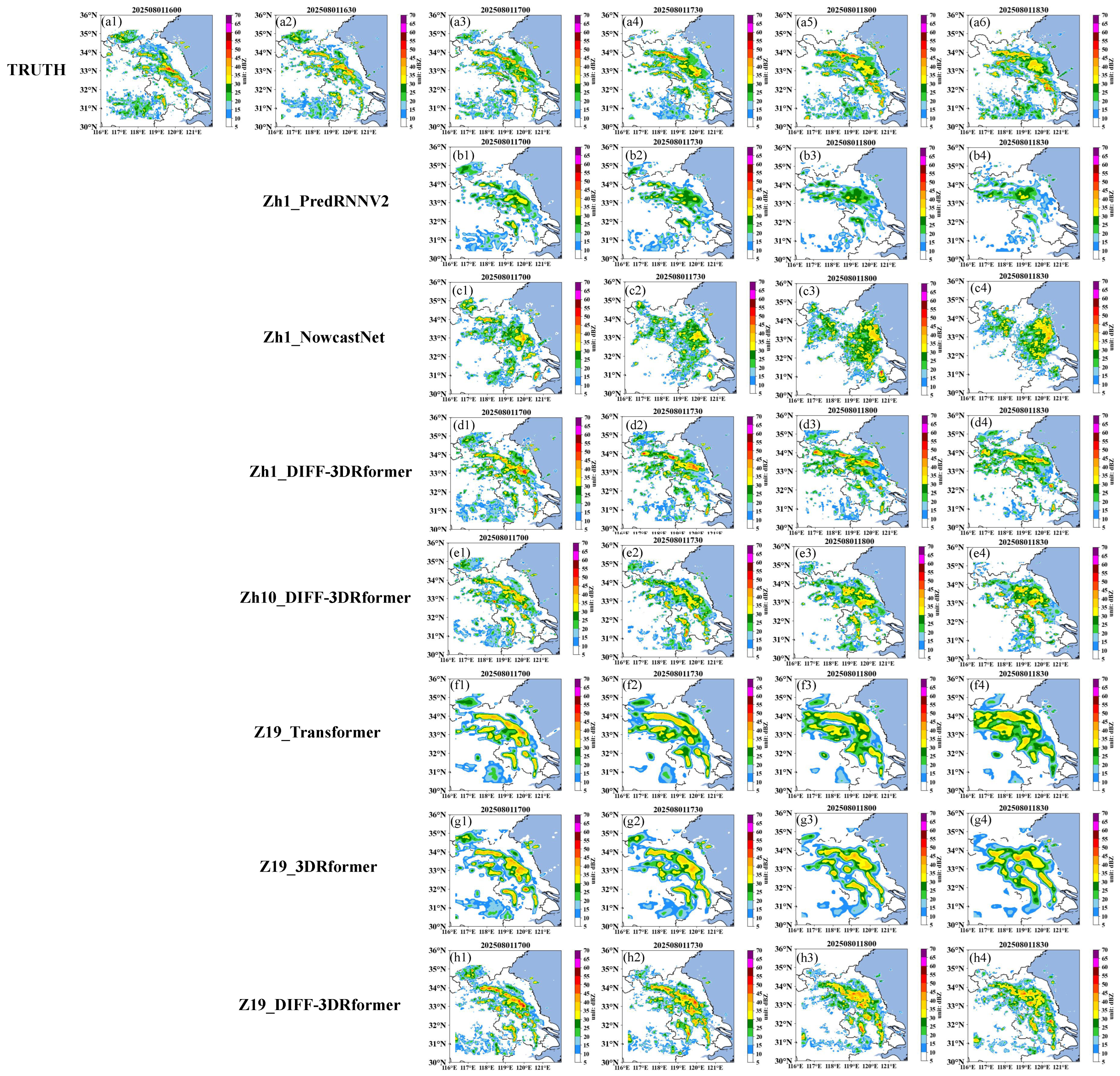
Figure 6 presents the observed (a1–a6) and prediction from three sets of controlled experimental models during a spiral rainband event associated with a typhoon over Jiangsu Province from 16:36 to 18:30 BT on 1 August 2025. Observations (a4–a6) reveal a localized enhancement of strong convection in the Suzhou area starting at 17:30 BT. Zh1_PredRNNV2 and Zh1_NowcastNet exhibit limited skill in predicting the morphology of typhoon spiral rainbands, while Zh1_DIFF-3DRformer better reproduces the spiral-band structure but shows notable discrepancies in the placement of intense radar reflectivity cores relative to observations. These results indicate that, among the three models, Zh1_DIFF-3DRformer more accurately captures the structural characteristics of typhoon spiral rainbands. Zh1_DIFF-3DRformer, Zh10_DIFF-3DRformer, and Zh19_DIFF-3DRformer all reproduce the morphological characteristics of spiral rainbands reasonably well. Among them, the positions of convective storms predicted by Zh19_DIFF-3DRformer are closest to the observed results, followed by Zh10_DIFF-3DRformer. These results indicate that increasing the number of radar echo input levels can improve the nowcasting accuracy of convective storm position, and the magnitude of performance improvement increases with the number of input levels. The Zh19_Transformer experiment captures the overall structure of the spiral rainband reasonably well at 17:00 (f1) and 17:30 (f2). However, as the forecast lead time increases, its ability to reproduce the rainband morphology deteriorates, and it fails to predict the short-term intense convection over Suzhou. In contrast, the Zh19_3DRformer, which incorporates physical constraints into the Zh19_transformer framework, shows a marked improvement in predicting the morphology of the spiral rainbands, although the convective intensity is notably underestimated compared to observations. This suggests that introducing physically constrained neural operators enhances the model’s capability in capturing the structure of strong convective echoes. Furthermore, the Zh19_DIFF-3DRformer, which integrates a diffusion model into the Zh19_3DRformer, not only successfully captures the localized strong convection over Suzhou but also substantially mitigates the underestimation of convective intensity seen in the physical-constraint-only experiment.

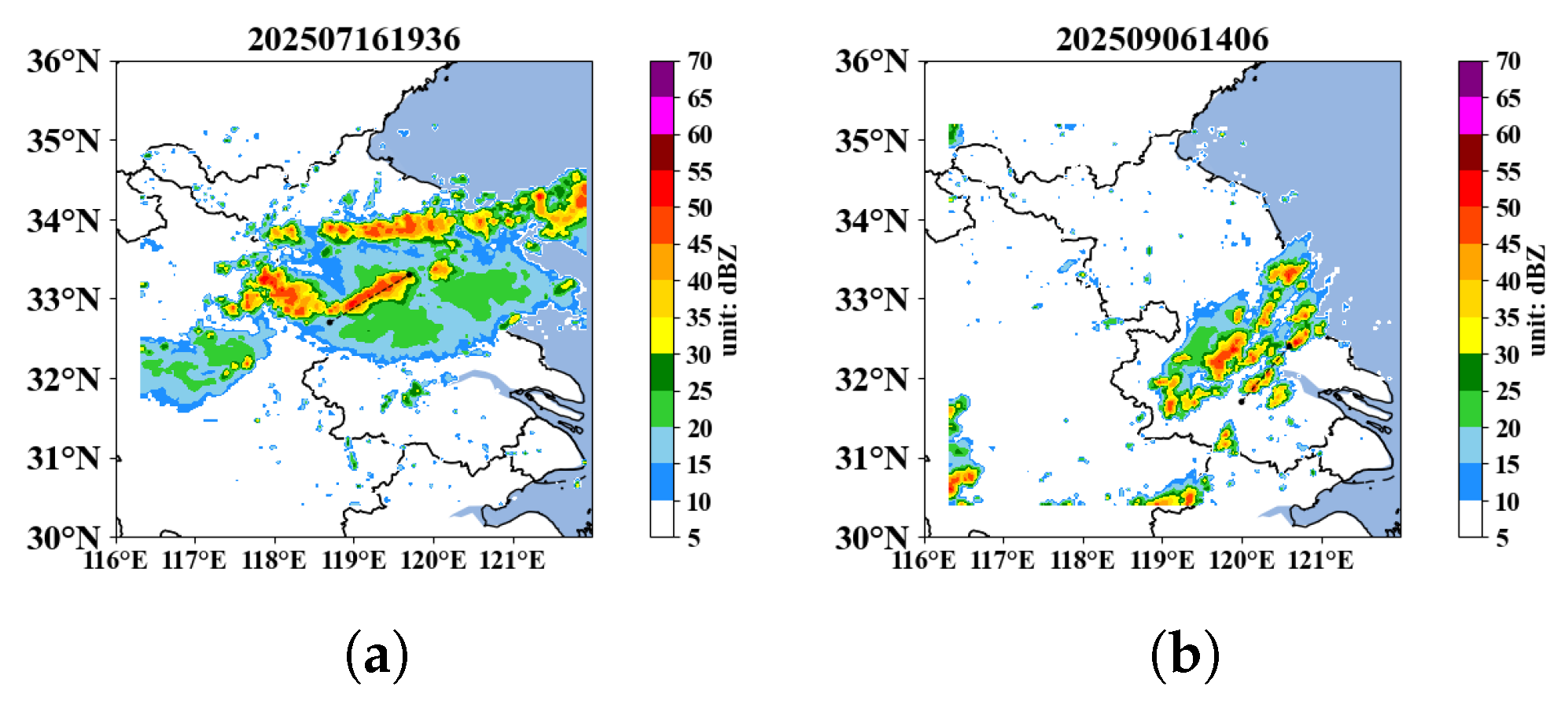
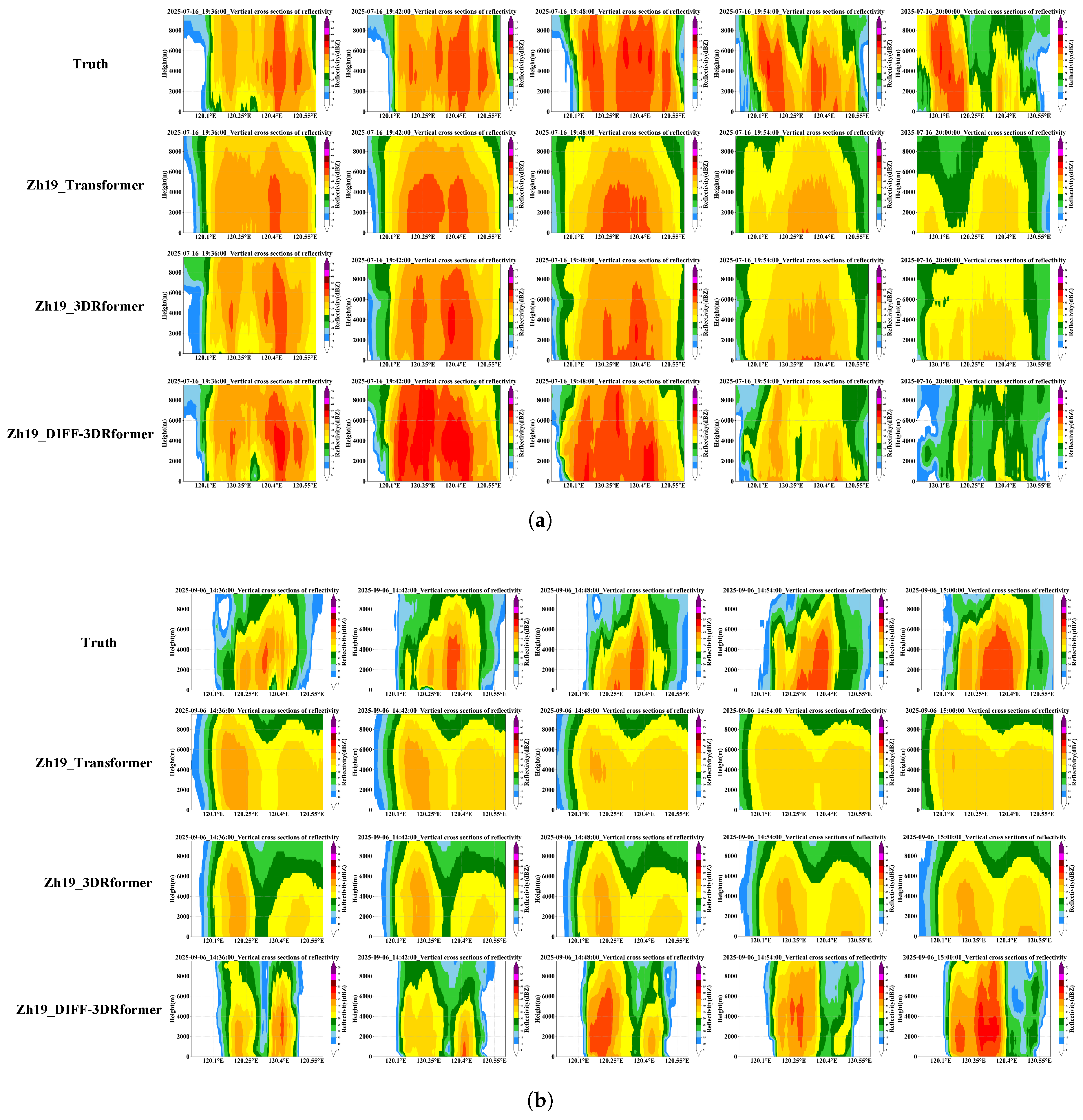
Furthermore, as some experimental designs in the first and second controlled experiment lacked forecast data for the 19 levels of reflectivity, the third control experiment was selected to demonstrate the model’s capability in capturing the three-dimensional evolution of storms. Vertical cross-sections of reflectivity factor forecasts are presented for the widespread squall line event on 16 July 2025 and the convective initiation case on 6 September 2025. To better visualize the three-dimensional storm development near the locations of convective initiation, vertical cross-sections along the transects defined by the two latitude–longitude points marked in Figure 7a and Figure 7b are shown for the 16 July and 6 September cases, respectively.

Figure 8 presents three-dimensional vertical cross-section forecasts from two representative cases. As shown in Figure 8a, from 19:36 to 19:48, all three models successfully capture the vertical structure of the convective storm. However, the Zh19_Transformer model forecasts the strong convective storm core with reflectivity above 50 dBZ only up to approximately 6000 m, whereas observations indicate that the storm core reaches beyond 9000 m. In contrast, the Zh19_3DRformer and Zh19_DIFF-3DRformer models produce storm core heights that align more closely with observations. Figure 8b illustrates a rapidly intensifying convective storm with an ascending core. Observations reveal that starting from 14:42, the storm begins to strengthen, and its core height gradually exceeds 6000 m. The Zh19_Transformer model fails to capture this intensification and ascent. The Zh19_3DRformer model reproduces the vertical structure of the storm but with underestimated intensity and some displacement in the core location. Notably, the Zh19_DIFF-3DRformer model accurately captures the ascending motion of the storm, despite a slight positional offset in the core region.

3.2. Quantitative Performance Evaluation

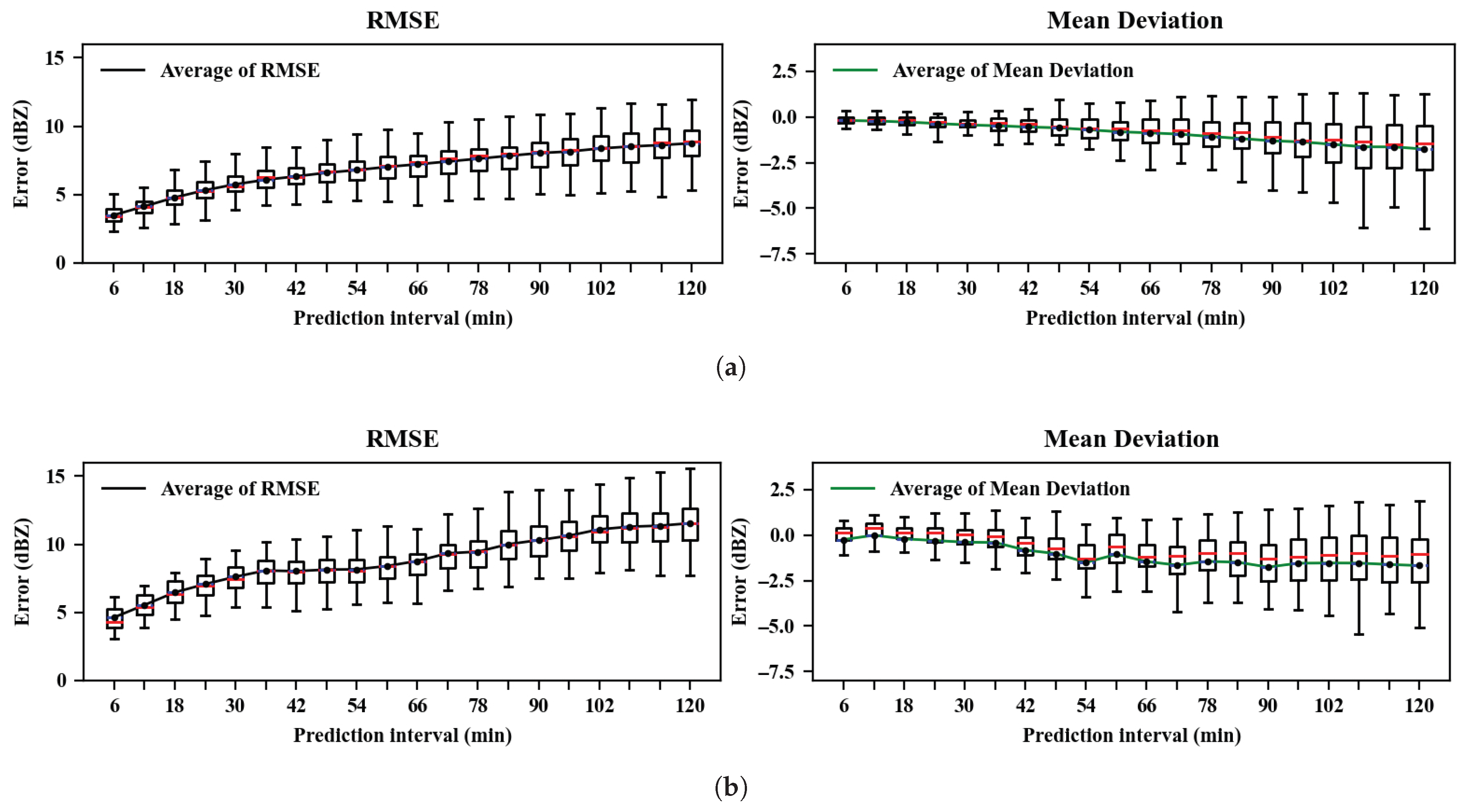
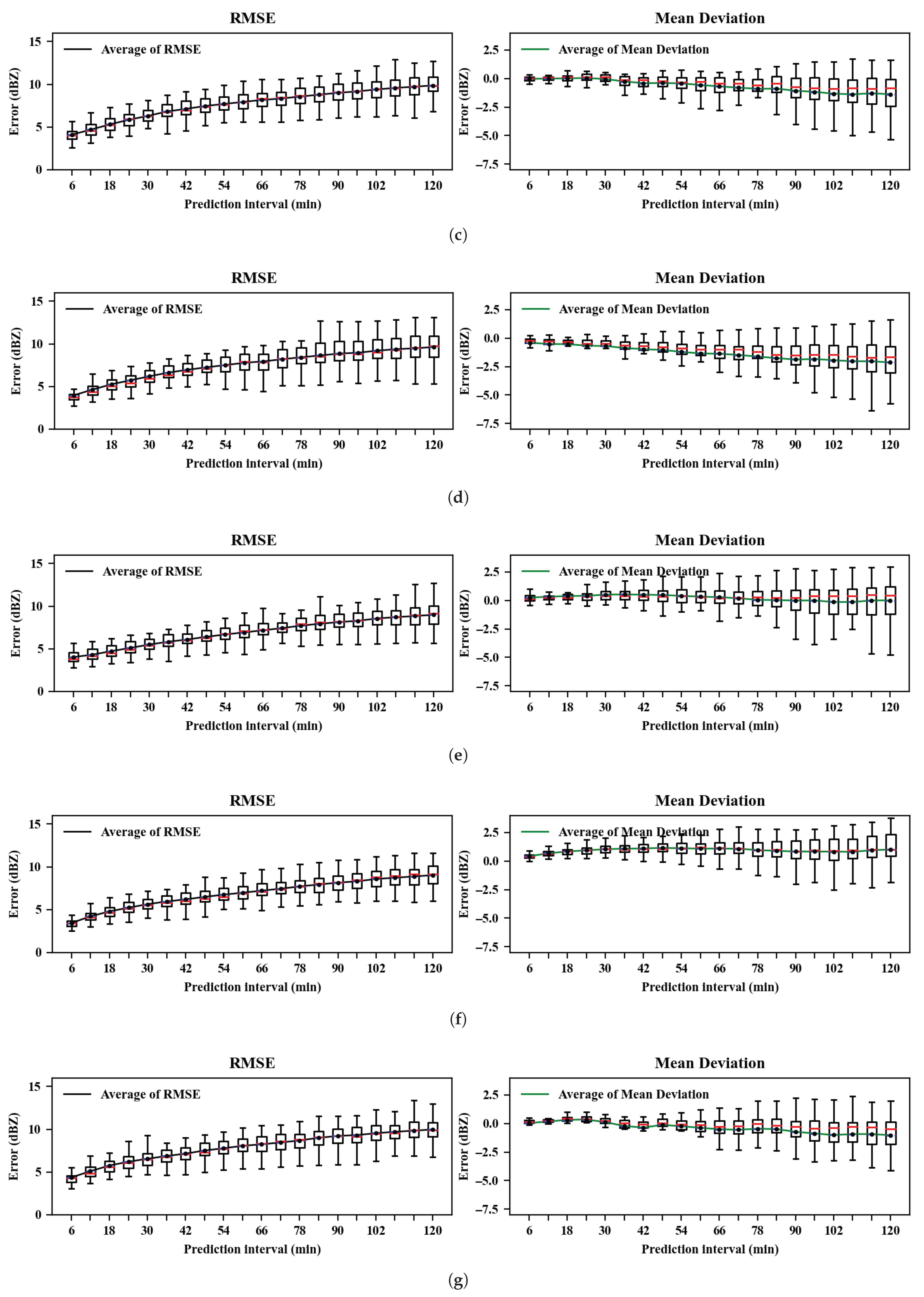
As illustrated in Figure 9, the root-mean-square error (RMSE) of the reflectivity factor for Zh1_NowcastNet(b) rises sharply starting from the 60th min, and after the 90th min, the overall RMSE exceeds 10 dBZ. In contrast, the RMSE values of Zh1_PredRNNV2(a) and Zh1_DIFF-3DRformer(c) increase gradually with time steps, and the errors at the 120th min remain below 10 dBZ. This phenomenon can be attributed to the fact that the PredRNNV2 model is inherently trained with the mean squared error (MSE) as the loss function, whereas NowcastNet adopts generative adversarial network (GAN) training, whose loss function incorporates multiple terms such as cumulative consistency loss, adversarial loss, and pooling loss. For the DIFF-3DRformer model, its loss function includes both MSE loss and denoising loss. Furthermore, the mean deviation (MD) of all three models are less than 0, indicating that they all underestimate the echo intensity. Notably, the overall mean bias of DIFF-3DRformer is lower, which demonstrates the superiority of the DIFF-3DRformer model over the other two counterparts. Zh1_DIFF-3DRformer, Zh10_DIFF-3DRformer, and Zh19_DIFF-3DRformer are similar, with all errors remaining below 10 dBZ at the 120th min. From the perspective of the mean deviation, the MD of Zh19_DIFF-3DRformer is close to 0 before the 60th min, and its error growth trend changes more slowly with time steps compared to Zh1_DIFF-3DRformer and Zh10_DIFF-3DRformer. This result confirms the effectiveness of increasing the input layers of radar echoes in reducing forecast errors. The mean bias of Zh19_Transformer becomes less than 0 after the 72nd min, while that of Zh19_3DRformer remains greater than 0 throughout the forecast period. Specifically, the mean bias of Zh19_3DRformer is close to 0 in the first 60 min but turns negative in the later stage. This observation can be explained by the introduction of physical constraints, which may lead to overestimation of forecast results in some weak echo areas. Additionally, the incorporation of the diffusion model results in a larger mean bias compared to the schemes trained without the diffusion model.

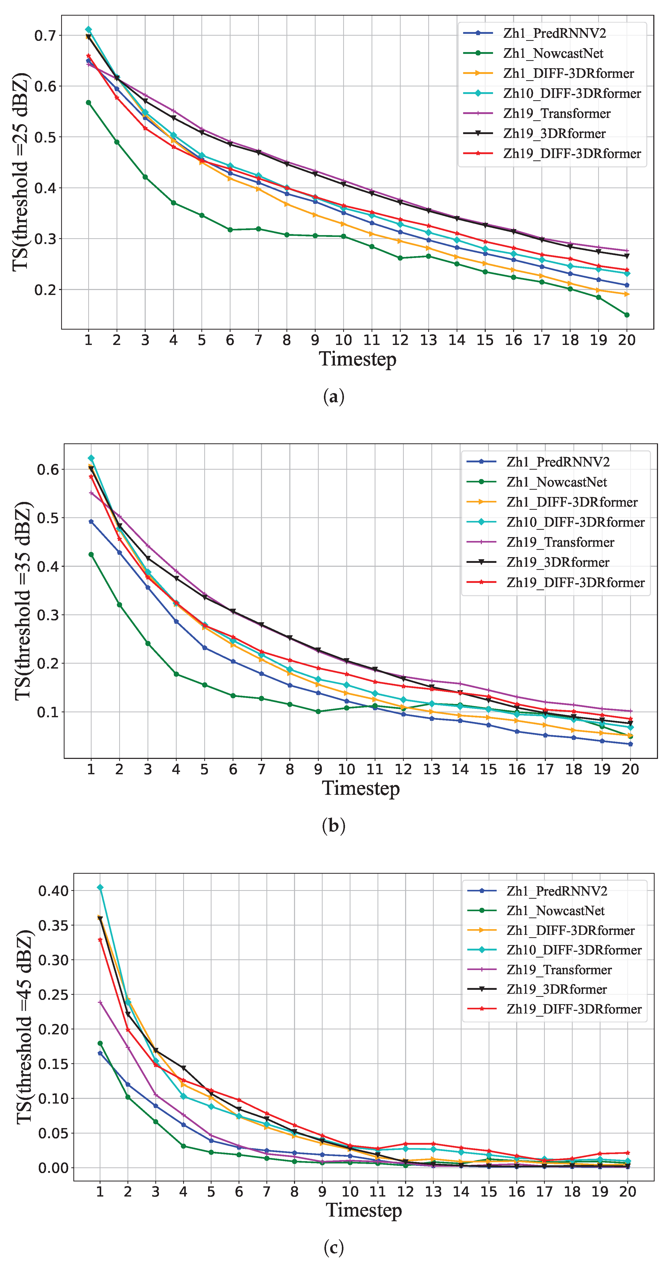
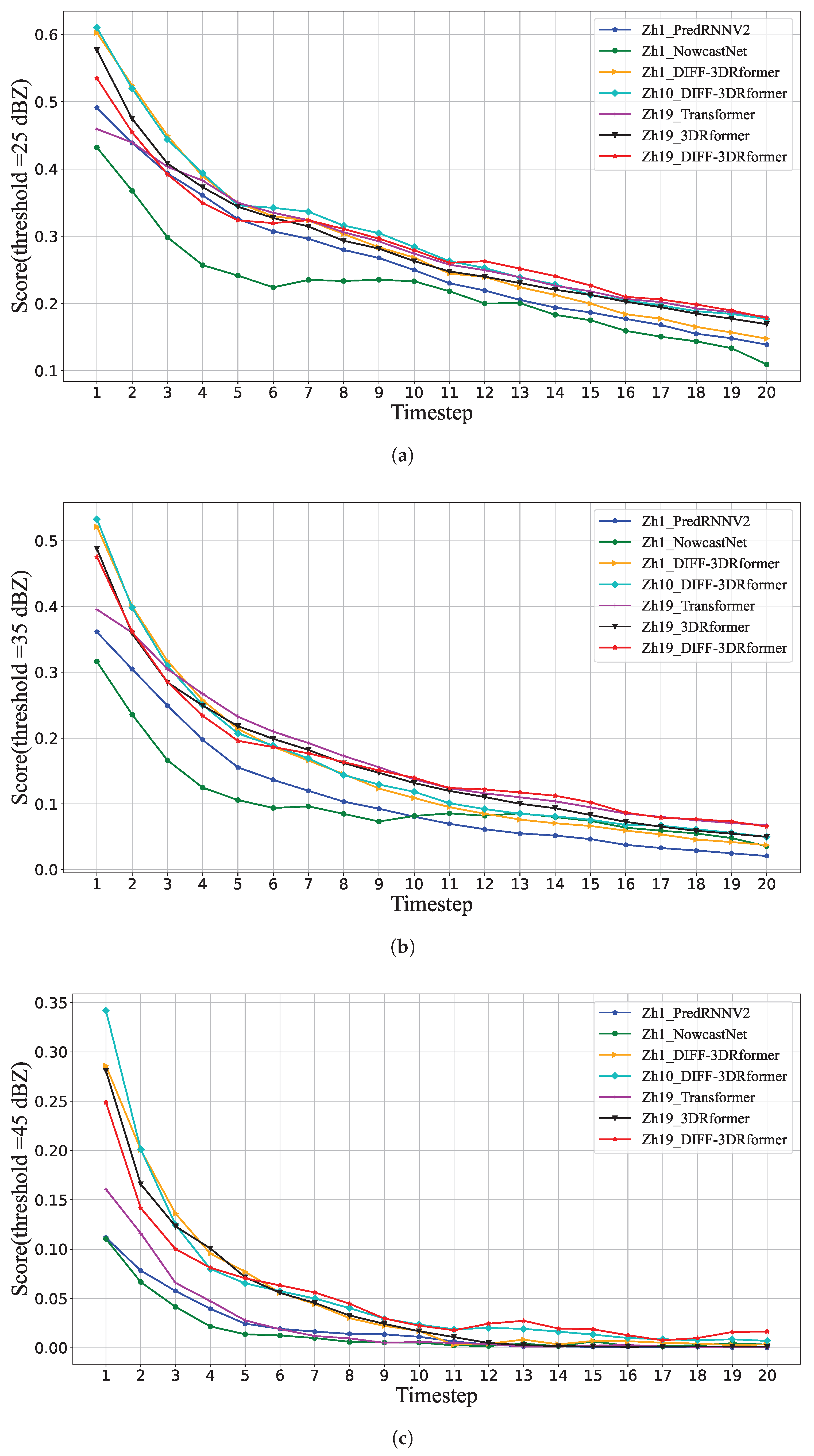
Figure 10 presents the variation in TS scores with forecast lead time during the test period (April–September 2025) for three sets of comparative experiments. As shown in Figure 10a, at the 25 dBZ threshold, Zh19_Transformer and Zh19_3DRformer achieve the best performance, with Zh19_3DRformer slightly outperforming Zh19_Transformer, followed by Zh19_DIFF-3DRformer. This is attributed to the fact that both Zh19_Transformer and Zh19_3DRformer adopt the mean squared error (MSE) as the loss function, which yields superior forecasting results for large-scale weak precipitation echoes. In addition, Zh1_DIFF-3DRformer, Zh10_DIFF-3DRformer, and Zh19_DIFF-3DRformer exhibit comparable forecasting performance within the first 36 min. However, after 36 min, the TS of Zh1_DIFF-3DRformer gradually becomes lower than that of Zh10_DIFF-3DRformer, while the TS of Zh10_DIFF-3DRformer also decreases progressively compared with Zh19_DIFF-3DRformer. The aforementioned results also indicate that increasing the input levels of radar echoes can extend the forecasting lead time of weak precipitation echoes. Across all time steps, the TS of Zh1_NowcastNet is consistently lower than those of Zh1_PredRNNV2 and Zh1_DIFF-3DRformer. Moreover, the TS of Zh1_PredRNNV2 becomes higher than that of Zh1_DIFF-3DRformer after 30 min. This is because the forecasting results of Zh1_PredRNNV2 gradually become blurred and averaged after 30 min, which enhances its performance in forecasting weak precipitation echoes. In contrast, Zh1_DIFF-3DRformer produces more refined forecasts, particularly demonstrating superior performance in predicting small-scale strong echoes.

As shown in Figure 10b, at the 35 dBZ threshold, starting from 18 min, the TS values of both Zh19_3DRformer and Zh19_DIFF-3DRformer are higher than those of other experimental schemes. This indicates that the introduction of physical constraints can improve the forecasting performance of convective storms. Furthermore, after 72 min, the TS of Zh19_DIFF-3DRformer gradually surpasses that of Zh19_3DRformer, which is due to the further integration of a diffusion model in Zh19_DIFF-3DRformer, effectively extending the forecasting lead time. Within the 0–72 min forecast range, the TS scores of Zh1_DIFF-3DRformer are significantly higher than those of the other two models. Beyond 72 min, however, Zh1_NowcastNet begins to outperform the others, which can be attributed to its use of generative ensemble forecasting. This approach enhances prediction stability and accuracy, allowing Zh1_NowcastNet to maintain reasonable skill in capturing the initiation and dissipation of storms beyond their typical lifecycle, thereby stabilizing TS scores.

Figure 10c displays TS scores for reflectivity ≥ 45 dBZ. At the 45 dBZ threshold, starting from 30 min, the TS of Zh19_DIFF-3DRformer is consistently superior to those of all other experimental schemes. Additionally, Zh19_DIFF-3DRformer and Zh19_3DRformer maintain higher TS values in the early forecasting stage. After 66 min, the TS values of Zh10_3DRformer and Zh19_DIFF-3DRformer are higher than those of other models. This indicates that in the late forecasting stage, the introduction of physical constraints alone is insufficient to improve the forecasting performance of severe convective storms, and the integration of a diffusion model is necessary to extend the forecasting lead time.

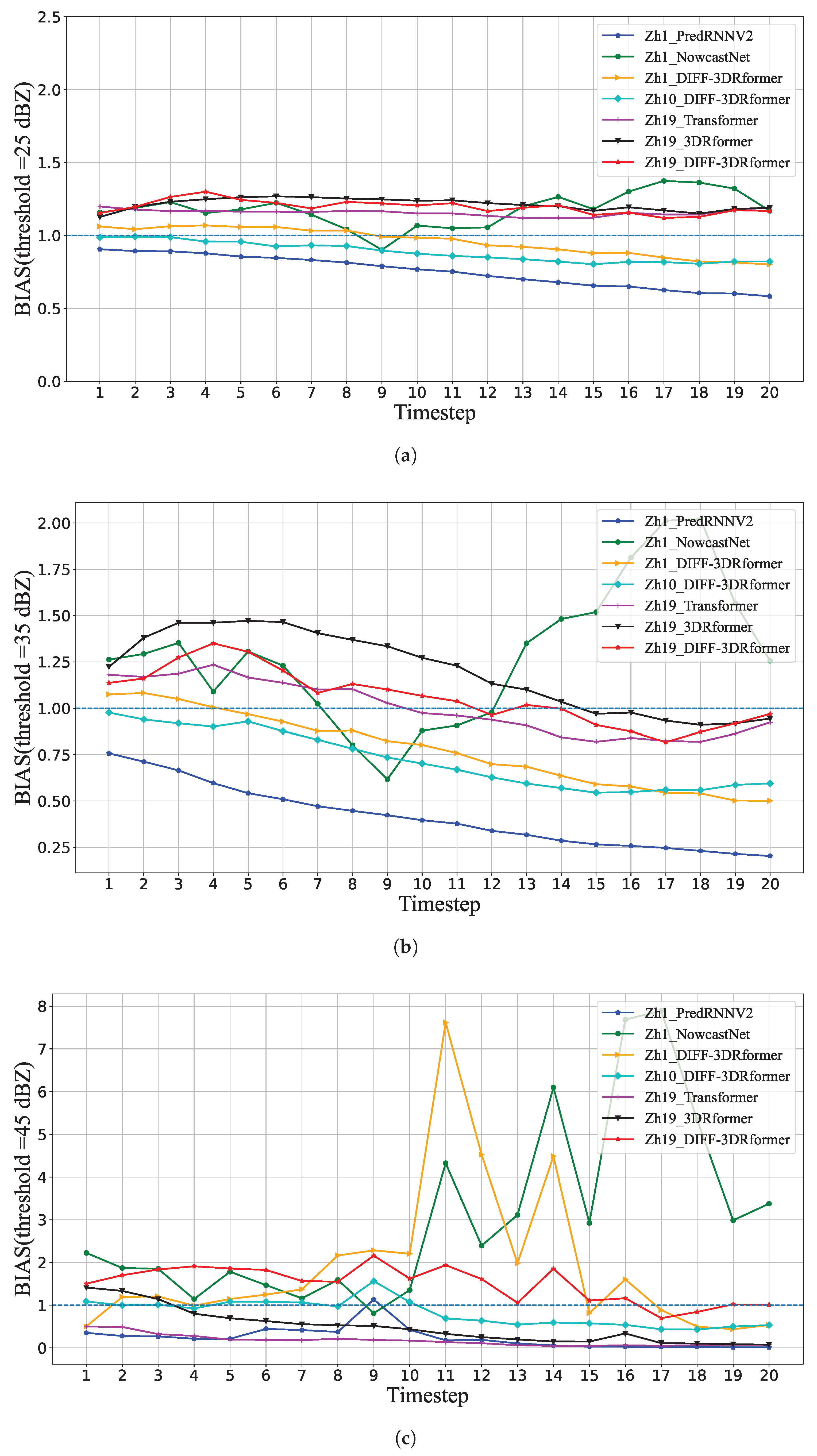
As illustrated in Figure 11, at the 25 dBZ threshold, Zh19_DIFF-3DRformer achieves the optimal performance within the first 66 min. In the later stage of the forecast, Zh1_PredRNNV2 exhibits the largest bias. At the 35 dBZ threshold, Zh19_Transformer, Zh19_3DRformer, and Zh19_DIFF-3DRformer demonstrate superior BIAS performance. This indicates that utilizing the maximum 19 levels of radar echo input can improve the BIAS score in the later forecast period. At the 45 dBZ threshold, after the 90th min, the BIAS score of Zh19_DIFF-3DRformer approaches 1, verifying its effectiveness in severe convective storm forecasting.

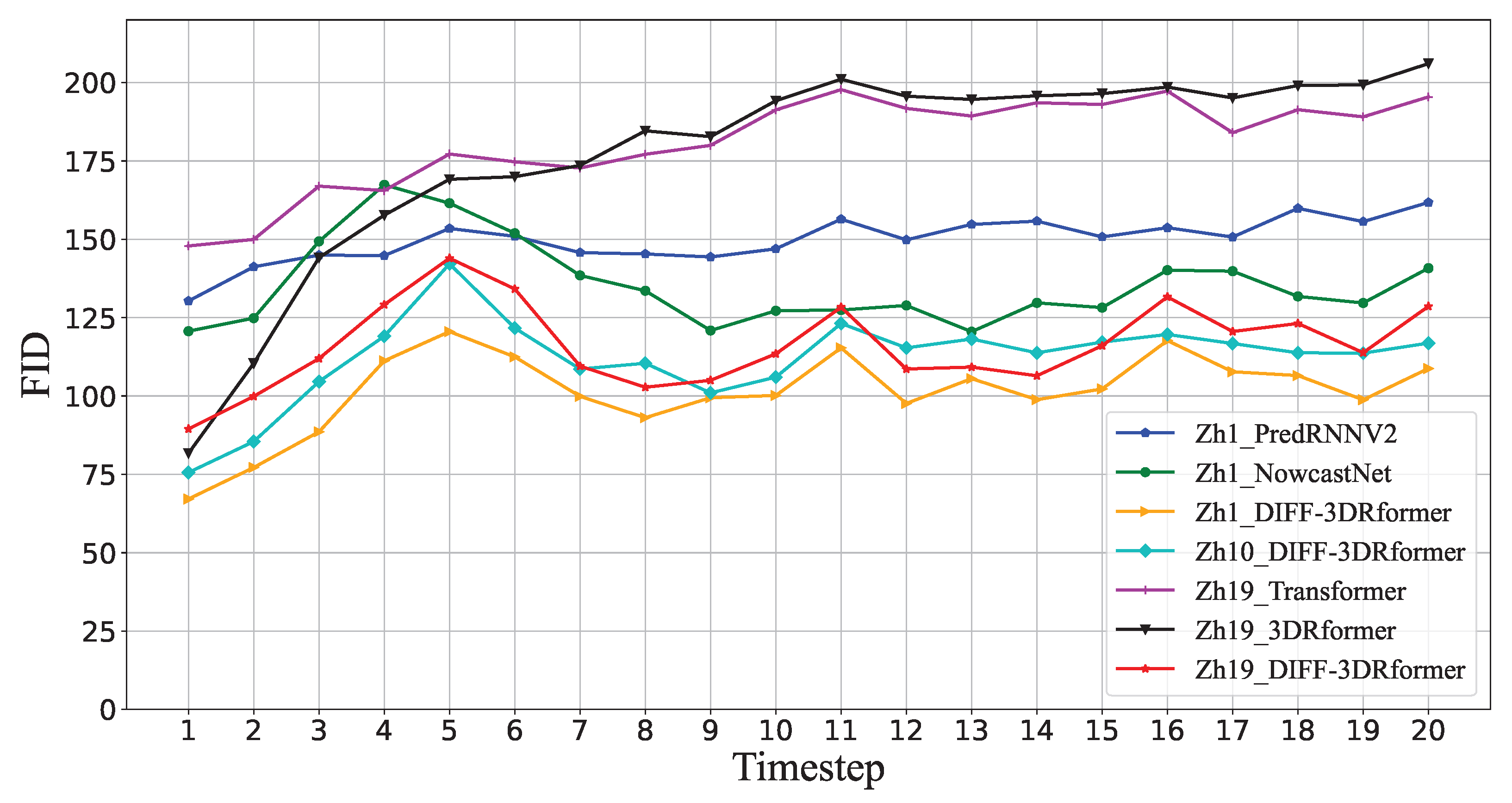
It is evident from Figure 12 that the three experimental schemes adopting the diffusion model, namely Zh1_DIFF-3DRformer, Zh10_DIFF-3DRformer and Zh19_DIFF-3DRformer, yield better performance. This confirms that the introduction of the diffusion model can enhance the clarity of forecast results.

Figure 13 presents the time-series variation curves of Score for various experimental schemes. At the 25 dBZ and 35 dBZ thresholds, Zh19_DIFF-3DRformer outperforms other schemes in terms of Score after the 72nd min. Additionally, at the 35 dBZ threshold, Zh19_Transformer, Zh19_3DRformer, and Zh19_DIFF-3DRformer achieve higher scores in the later forecast stage, suggesting that increasing the number of radar echo input levels can improve the late-stage forecast performance. At the 45 dBZ threshold, Zh19_3DRformer consistently outperforms Zh19_Transformer, while Zh1_PredRNNV2 and Zh1_NowcastNet exhibit the worst metrics. This not only validates the effectiveness of the introduced physical constraints but also demonstrates that the proposed DIFF-3DRformer model is superior to the mainstream extrapolation models PredRNNV2 and NowcastNet.

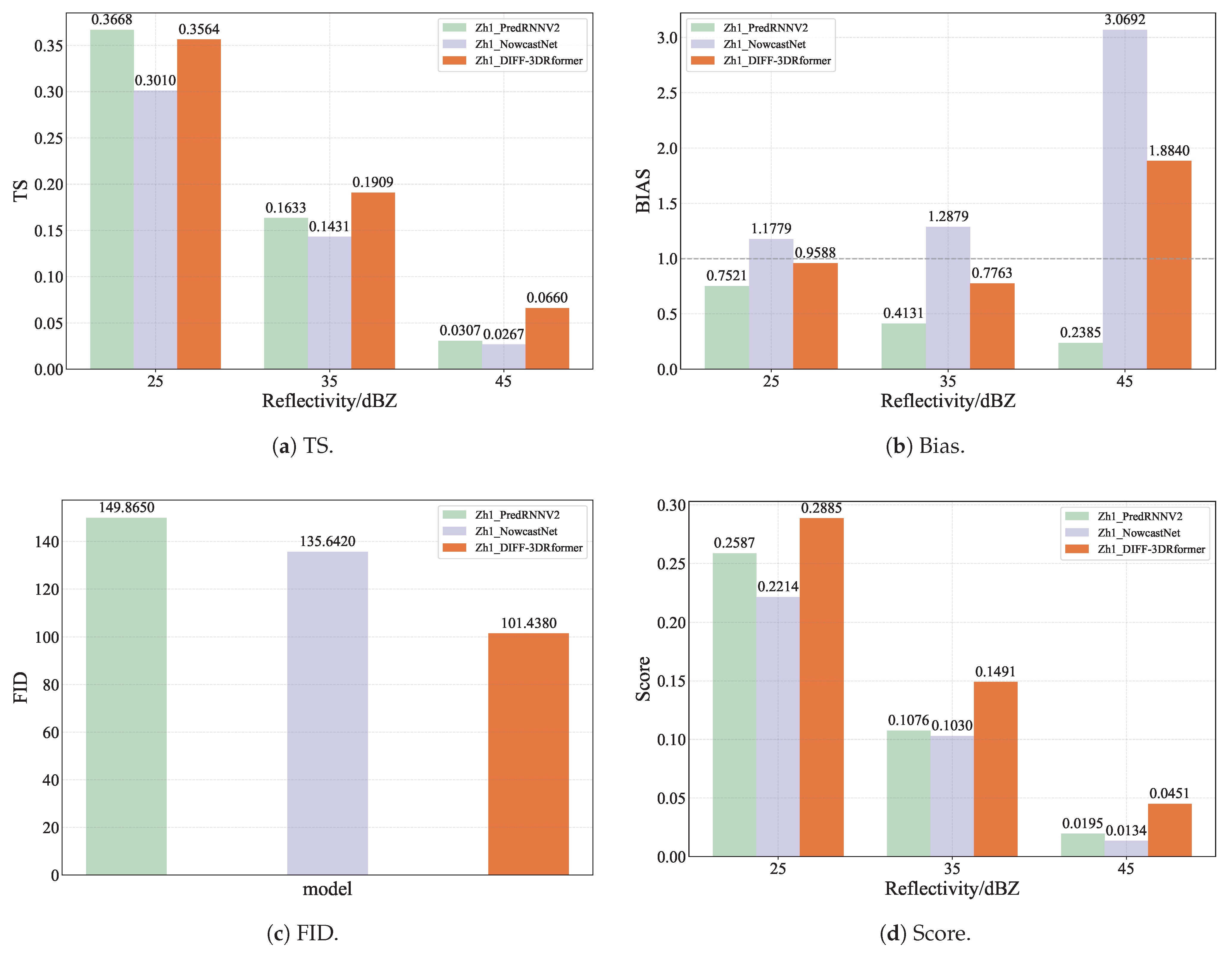
In addition, the 0–2 h TS, Bias, FID and Score of the three comparative experimental schemes were evaluated. As illustrated in Figure 14a, Zh1_DIFF-3DRformer exhibits higher TS values for convective echoes (≥35 dBZ) at 0–2 h lead times compared to the PredRNNV2 and NowcastNet models. Notably, for intense convective echoes (≥45 dBZ), the TS of Zh1_DIFF-3DRformer is 0.0353 higher than that of NowcastNet, indicating a more pronounced advantage in forecasting extreme convective weather. In terms of BIAS (Figure 14b), the BIAS of NowcastNet deviates substantially from 1 at the ≥45 dBZ threshold, while PredRNNV2 shows BIAS values between 0.2 and 0.8 across all thresholds, suggesting a systematic underestimation of echo area. In contrast, DIFF-3DRformer demonstrates superior BIAS performance. Regarding the FID metric (Figure 14c), both NowcastNet and DIFF-3DRformer, which employ generative artificial intelligence techniques, yield sharper forecasts than PredRNNV2, with DIFF-3DRformer achieving the optimal FID score. The composite Score results (Figure 14d), reveal that DIFF-3DRformer outperforms NowcastNet by 30.3%, 44.8%, and 236.6% at the ≥25 dBZ, ≥35 dBZ, and ≥45 dBZ thresholds, respectively. These results demonstrate that, using single-layer composite reflectivity data as input, DIFF-3DRformer achieves overall superior scores compared to both PredRNNV2 and NowcastNet.

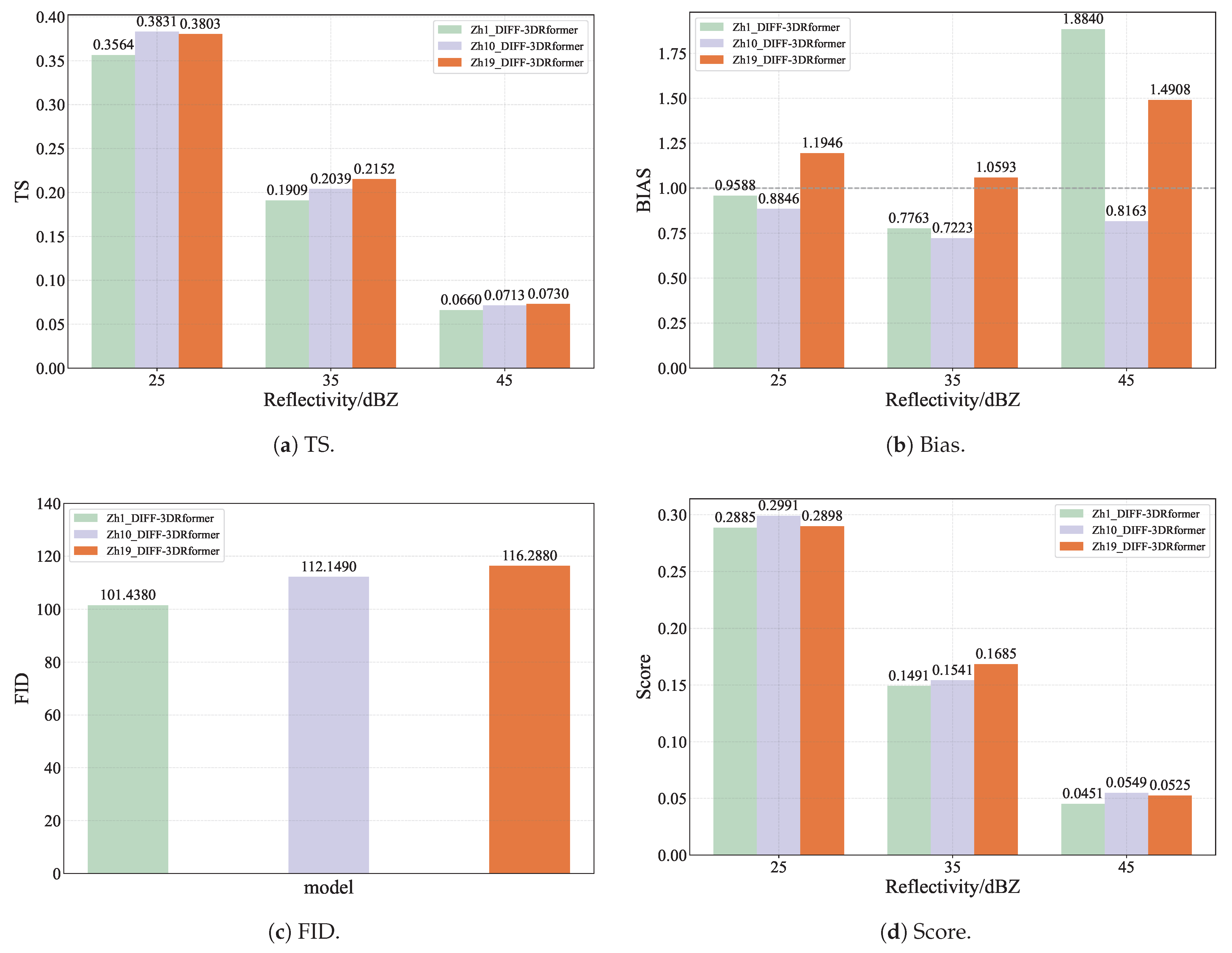
As illustrated in Figure 15a, the Zh19_DIFF-3DRformer model exhibits higher TS scores for thresholds ≥35 dBZ and ≥45 dBZ at 0–2 h lead times compared to the Zh10_DIFF-3DRformer, and also outperforms the Zh1_DIFF-3DRformer. In terms of Bias score (Figure 15b) Zh19_DIFF-3DRformer, which utilizes 19 levels of radar reflectivity as input, shows Bias scores close to 1 for thresholds ≥25 dBZ and ≥35 dBZ. Regarding the FID metric (Figure 15c), since the three experimental setups output extrapolation results at different levels, the scheme employing more input levels needs to predict more output levels. This makes the model learning process more complex compared to the single-level input and output approach. Consequently, using more input levels can lead to a degradation in FID score. Based on the comprehensive Score results (Figure 15d), using more radar echo layers as input improves the Score for thresholds ≥35 dBZ (convective echoes). This suggests that using additional vertical echo levels can improve the forecast skill for convective systems.

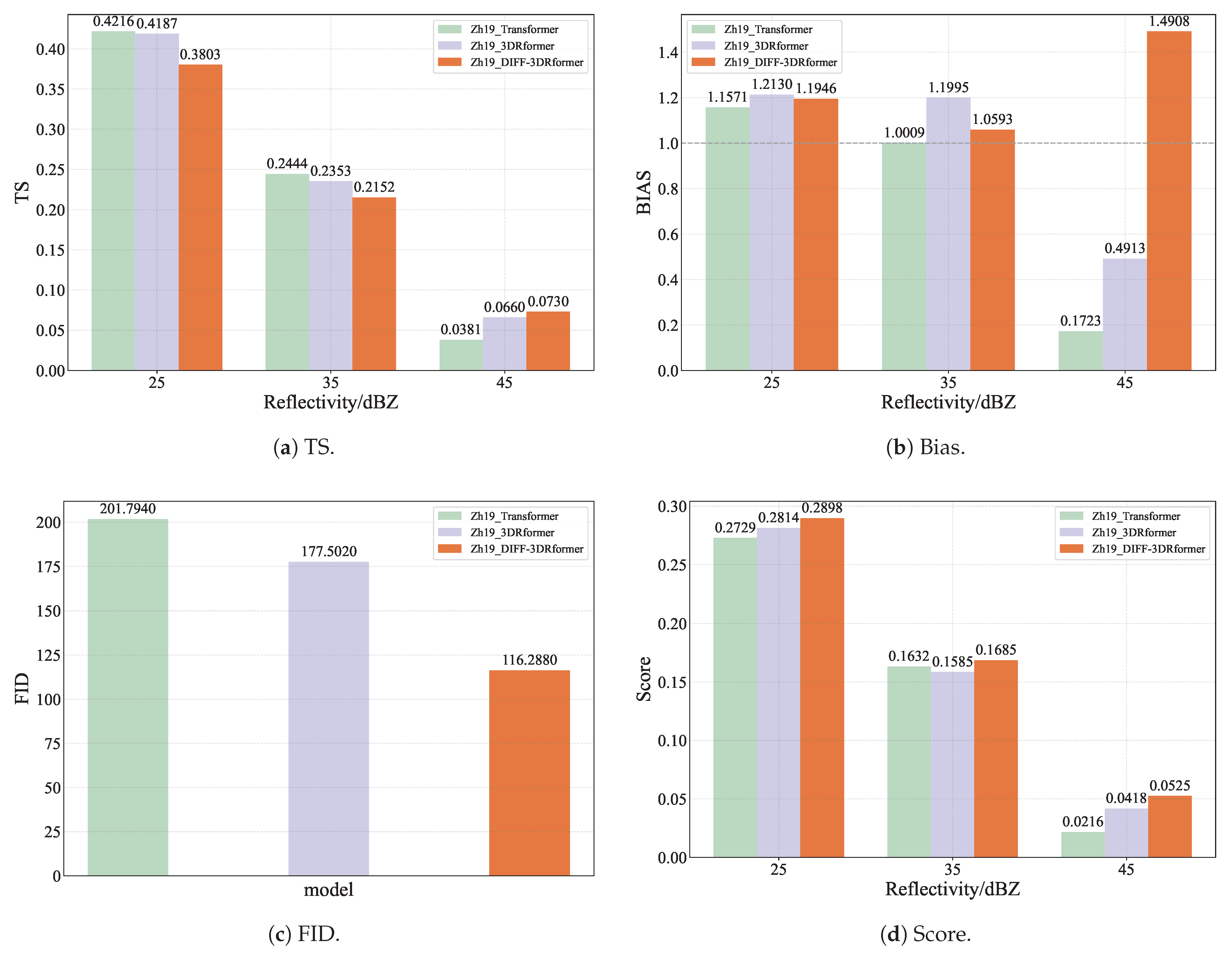
As illustrated in Figure 16, the Zh19_3DRformer scheme, which integrates physical constraint neural operators, achieves TS that are comparable to or slightly lower than those of the Zh19_Transformer baseline at the 25 dBZ and 35 dBZ thresholds across a 0–2 h forecast lead time. However, a marked improvement is observed at the more intense convective echo threshold (≥45 dBZ), where the Zh19_3DRformer yields a 73.2% increase in TS relative to the Zh19_Transformer. This enhancement can be attributed to the incorporated physical neural operators, which are primarily designed to represent updraft motions within strong convective systems. By jointly optimizing the root mean square error and divergence loss, the scheme prioritizes the accurate representation of intense convection, albeit with a minor trade-off in skill for weaker echoes compared to a loss function relying solely on mean squared error. Furthermore, the addition of a convective-scale denoising diffusion model provides a secondary, albeit smaller, boost to the TS at the ≥45 dBZ. In terms of Bias score (Figure 16b), the integration of physical constraints also leads to improved performance specifically for strong convective echoes. Regarding the FID (Figure 16c), both the Zh19_Transformer and Zh19_3DRformer yield similar results, as neither employs generative deep learning models to enhance extrapolation sharpness. Notably, augmenting the Zh19_3DRformer with the convective-scale diffusion model significantly reduces the FID score, indicating a substantial gain in the spatial clarity and realism of the forecast fields. The comprehensive scoring results (Figure 16d) confirm that at the ≥45 dBZ threshold, the Zh19_DIFF-3DRformer configuration outperforms the other experimental schemes. In summary, the inclusion of physics-constrained neural operators effectively improves the forecast skill for intense convective echoes, and this benefit is further augmented by the application of a diffusion model, which markedly enhances the structural sharpness of the extrapolation results.

4. Discussion

Weather radar provides high spatiotemporal resolution and is a key observational tool for monitoring severe convective weather. Radar echo extrapolation leverages historical echo sequences to predict the evolution of storm motion, development, and dissipation, thereby supporting timely warnings for short-duration heavy rainfall, thunderstorm gusts, hail, and other high-impact convective hazards. Conventional single-level echo extrapolation methods, however, struggle to represent the complex, nonlinear life cycles of convective storms in three-dimensional (3D) space; in contrast, 3D extrapolation better captures vertical structure and interlevel physical relationships. In addition, some deterministic deep learning extrapolation models that rely on average reconstruction losses, such as the mean squared error (MSE) or mean absolute error (MAE), tend to produce overly smoothed forecasts to minimize loss, which in turn leads to a systematic underestimation of intense convective echoes. Moreover, echo fields at different height levels are not independent, they are coupled by physical constraints.

To address these challenges, we propose a 3D echo extrapolation framework that integrates a spatiotemporal Transformer with an advection neural operator and a 3D continuity equation loss to explicitly enforce mass continuity. Building on this physically constrained formulation, we further incorporate a convection-scale denoising generative model to better resolve fine-scale convective structures. We compare our model against mainstream baselines, including PredRNNV2 and NowcastNet, and conduct experiments to assess the impact of varying the number of input radar echo levels. Ablation studies are designed to quantify the benefits of the physics-based continuity loss and the diffusion-based denoising generator. The proposed model adopts an end-to-end architecture; during diffusion training, we employ DDIMs (Deterministic Denoising Implicit Models) to accelerate sampling. As reported in

Table 2. The details of training and inference time and memory consumption.

Training Time/Epoch	Training Memory Consumption	Inference Time	Inference Memory Consumption
2.8 h	32,451 Mib	15.3 s	4751 Mib

, the model achieves a single-sequence inference time of only 15.3 s, satisfying the stringent latency requirements of severe convective nowcasting. Overall, the proposed approach improves the accuracy of short-term convective forecasts and demonstrates the substantial potential of intelligent meteorology.

5. Conclusions

This study introduces DIFF-3DRformer, a novel deep learning model based on three-dimensional radar reflectivity for the nowcasting of severe convective storms. The proposed model enhances the Forecastformer architecture—which consists of a mesoscale evolution network and a convective-scale denoising generation network—by incorporating a 3D advection neural operator and integrating a loss term constrained by the 3D continuity equation. These improvements optimize the mesoscale evolution network, leading to the developed 3DRformer that more effectively captures the three-dimensional structure of severe convective storms and simulates their initiation, development, and motion. Combined with a diffusion model-based convective-scale denoising generation network, the approach improves the prediction of reflectivity intensity at convective scales.

Quantitative evaluation and case study analyses lead to the following conclusions. Assessments based on representative severe convective events in 2025 indicate that DIFF-3DRformer exhibits certain capabilities in forecasting the evolution of convection across different convective scales. Using additional radar elevation levels as input significantly improves the morphology and intensity predictions of convective echoes, while the incorporation of physical constraints further refines echo structure and spatial placement. Quantitative tests on the April–September 2025 dataset show that DIFF-3DRformer overall outperforms the PredRNNV2 and NowcastNet models. Increasing the number of radar elevation levels improves the convective echo forecasting to some extent, and embedding the physics-constrained neural operator enhances the prediction of intense reflectivity cores (≥45 dBZ). Furthermore, the addition of the diffusion model substantially sharpens the forecast details.

This framework offers a viable solution for directly characterizing the 3D structure of convective storms. Moreover, the proposed model is not limited to 3D radar extrapolation, it can also be applied to other meteorological 3D fields, such as wind and temperature. While the current study focuses on nowcasting lead times of 0–2 h, extending the forecast horizon beyond 3 h will be necessary to meet evolving operational needs. High-resolution numerical weather prediction parameters are expected to provide more comprehensive structural information on environmental features. Integrating such additional variables into the model and developing multi-source data fusion methods will further enhance the accuracy and timeliness of severe convective storm nowcasting. These directions will be pursued in future work.

References

1. Shin, H.C.; Ha, J.H.; Ahn, K.D.; Lee, E.H.; Kim, C.H.; Lee, Y.H.; Clayton, A. An Overview of KMA’s Operational NWP Data Assimilation Systems. In Data Assimilation for Atmospheric, Oceanic and Hydrologic Applications (Vol. IV); Park, S.K., Xu, L., Eds.; Springer International Publishing: Cham, Switzerland, 2022; pp. 665–687. [Google Scholar] [CrossRef]
2. Park, J.; Lee, C. CPrecNet: Enhanced Nowcast of High-Resolution Short-Term Precipitation Using Deep Learning. Geophys. Res. Lett. 2025, 52, e2024GL113907. [Google Scholar] [CrossRef]
3. Rinehart, R.; Garvey, E. Three-dimensional storm motion detection by conventional weather radar. Nature 1978, 273, 287–289. [Google Scholar] [CrossRef]
4. Bowler, N.E.; Pierce, C.E.; Seed, A. Development of a precipitation nowcasting algorithm based upon optical flow techniques. J. Hydrol. 2004, 288, 74–91. [Google Scholar] [CrossRef]
5. Germann, U.; Zawadzki, I. Scale-Dependence of the Predictability of Precipitation from Continental Radar Images. Part I: Description of the Methodology. Mon. Weather. Rev. 2002, 130, 2859–2873. [Google Scholar] [CrossRef]
6. Chen, K.; Han, T.; Gong, J.; Bai, L.; Ling, F.; Luo, J.J.; Chen, X.; Ma, L.; Zhang, T.; Su, R.; et al. FengWu: Pushing the Skillful Global Medium-range Weather Forecast beyond 10 Days Lead. arXiv 2023, arXiv:2304.02948. [Google Scholar]
7. Espeholt, L.; Agrawal, S.; Sønderby, C.; Kumar, M.; Heek, J.; Bromberg, C.; Gazen, C.; Hickey, J.; Bell, A.; Kalchbrenner, N. Skillful Twelve Hour Precipitation Forecasts using Large Context Neural Networks. arXiv 2021, arXiv:2111.07470. [Google Scholar] [CrossRef]
8. Wang, Y.; Wu, H.; Zhang, J.; Gao, Z.; Wang, J.; Yu, P.S.; Long, M. PredRNN: A Recurrent Neural Network for Spatiotemporal Predictive Learning. IEEE Trans. Pattern Anal. Mach. Intell. 2023, 45, 2208–2225. [Google Scholar] [CrossRef] [PubMed]
9. Ayzel, G.; Scheffer, T.; Heistermann, M. RainNet v1.0: A convolutional neural network for radar-based precipitation nowcasting. Geosci. Model Dev. 2020, 13, 2631–2644. [Google Scholar] [CrossRef]
10. Zhou, K.; Zheng, Y.; Dong, W.; Wang, T. A Deep Learning Network for Cloud-to-Ground Lightning Nowcasting with Multisource Data. J. Atmos. Ocean. Technol. 2020, 37, 927–942. [Google Scholar] [CrossRef]
11. Franch, G.; Nerini, D.; Pendesini, M.; Coviello, L.; Jurman, G.; Furlanello, C. Precipitation Nowcasting with Orographic Enhanced Stacked Generalization: Improving Deep Learning Predictions on Extreme Events. Atmosphere 2020, 11, 267. [Google Scholar] [CrossRef]
12. Gao, Z.; Shi, X.; Wang, H.; Zhu, Y.; Wang, Y.B.; Li, M.; Yeung, D.Y. Earthformer: Exploring space-time transformers for earth system forecasting. Adv. Neural Inf. Process. Syst. 2022, 35, 25390–25403. [Google Scholar]
13. Zhuang, X.; Zheng, Y.; Wang, Y.; Kang, Z.; Min, J.; Zhang, W.; Li, Y. A deep learning-based fusion precipitation nowcast method and its application study in the eastern China. J. Meteorol. Res. 2023, 81, 286–303. [Google Scholar]
14. Shi, X.; Chen, Z.; Wang, H.; Yeung, D.Y.; Wong, W.K.; Woo, W.C. Convolutional lstm network: A machine learning approach for precipitation nowcasting. Adv. Neural Inf. Process. Syst. 2015, 28, 802–810. [Google Scholar]
15. Pan, X.; Lu, Y.; Zhao, K.; Huang, H.; Wang, M.; Chen, H. Improving Nowcasting of Convective Development by Incorporating Polarimetric Radar Variables Into a Deep-Learning Model. Geophys. Res. Lett. 2021, 48, e2021GL095302. [Google Scholar] [CrossRef]
16. Ravuri, S.; Lenc, K.; Willson, M.; Kangin, D.; Lam, R.; Mirowski, P.; Fitzsimons, M.; Athanassiadou, M.; Kashem, S.; Madge, S.; et al. Skilful precipitation nowcasting using deep generative models of radar. Nature 2021, 597, 672–677. [Google Scholar] [CrossRef]
17. Zhang, Y.; Long, M.; Chen, K.; Xing, L.; Jin, R.; Jordan, M.I.; Wang, J. Skilful nowcasting of extreme precipitation with NowcastNet. Nature 2023, 619, 526–532. [Google Scholar] [CrossRef] [PubMed]
18. Li, G.; Liu, L.; Lian, Z.; Zhou, M.; Li, Z. Statistical study of the identification of thunderstorm gale based on the radar 3D mosaic data. Acta Meteorol. Sin. 2014, 72, 1347–1355. [Google Scholar]
19. Wang, Z.; Qin, Y.; Zeng, L.; Zhang, R. High-Dynamic Radar Sequence Prediction for Weather Nowcasting Using Spatiotemporal Coherent Gaussian Representation. arXiv 2025, arXiv:2502.14895. [Google Scholar]
20. Zhang, W.; Han, L.; Sun, J.; Guo, H.; Dai, J. Application of Multi-channel 3D-cube Successive Convolution Network for Convective Storm Nowcasting. In Proceedings of the 2019 IEEE International Conference on Big Data (Big Data), Los Angeles, CA, USA, 9–12 December 2019; pp. 1705–1710. [Google Scholar] [CrossRef]
21. Tran, Q.K.; Song, S.k. Multi-Channel Weather Radar Echo Extrapolation with Convolutional Recurrent Neural Networks. Remote Sens. 2019, 11, 2303. [Google Scholar] [CrossRef]
22. Sun, N.; Zhou, Z.; Li, Q.; Jing, J. Three-Dimensional Gridded Radar Echo Extrapolation for Convective Storm Nowcasting Based on 3D-ConvLSTM Model. Remote Sens. 2022, 14, 4256. [Google Scholar] [CrossRef]
23. Ding, M.; Xiao, B.; Codella, N.; Luo, P.; Wang, J.; Yuan, L. Davit: Dual attention vision transformers. In Computer Vision—ECCV 2022; Springer: Cham, Switzerland, 2022; pp. 74–92. [Google Scholar]
24. Ho, J.; Jain, A.; Abbeel, P. Denoising diffusion probabilistic models. Adv. Neural Inf. Process. Syst. 2020, 33, 6840–6851. [Google Scholar]
25. Zhang, S.; Huang, X.; Min, J.; Chu, Z.; Zhuang, X.; Zhang, H. Improved fuzzy logic method to distinguish between meteorological and non-meteorological echoes using C-band polarimetric radar data. Atmos. Meas. Tech. 2020, 13, 537–551. [Google Scholar] [CrossRef]
26. Geng, L.; Min, J.; Geng, H.; Zhuang, X. Forecastformer: Spatiotemporal Decoupled Transformer and Diffusion Models for Severe Convective Storm Nowcasting. IEEE Trans. Geosci. Remote Sens. 2025, 63, 4108814. [Google Scholar] [CrossRef]
27. Liu, X.; Fu, X. On the derivation of continuity equation and several forms of transformation. Mech. Eng. 2023, 45, 469–474. [Google Scholar] [CrossRef]
28. Zeng, K.; Min, J.; Zhuang, X.; Kang, Z. Severe Convection Nowcasting Method Based on a Generative Adversarial Network and Its Application Evaluation in Eastern China. Chin. J. Atmos. Sci. 2024, 48, 2316–2328. [Google Scholar] [CrossRef]
Figure 1. Spatial Distribution of S-Band Dual-Polarization Radars in the Jiangsu Province, China. The red triangle denotes the center location of the radar station for the corresponding site.
Remotesensing 18 00206 g001
Figure 2. Schematic diagram of the DIFF-3DRformer model architecture, integrating mesoscale evolution and convective-scale denoising generation networks for three-dimensional radar echo extrapolation. The mesoscale evolution network learns the motion trends of mesoscale echoes, while the convective-scale denoising generative network simulates the relatively stochastic processes of convective-scale echo initiation and dissipation.
Remotesensing 18 00206 g002
Figure 3. 3DRformer architecture. The main pipeline and schematic depiction of 3DRformer encapsulate three essential components: a spatiotemporal encoder, dual decoders, and a 3D physical advection operator.
Remotesensing 18 00206 g003
Figure 4. A convective organization case from 14:06 to 16:00 Beijing Time on 6 September 2025. Reflectivity observations of input (a1,a2) and afterward ground truth (a3a6) and nowcasts from experiment Zh1_PredRNNV2 (b1b4), Zh1_NowcastNet (c1c4), Zh1_DIFF-3DRformer (d1d4), Zh10_DIFF-3DRformer (e1e4), Zh19_Transformer (f1f4), Zh19_3DRformer (g1g4) and Zh19_DIFF-3DRformer (h1h4). For models capable of predicting multi-layer radar echoes, the maximum vertical column reflectivity is displayed. Radar images are shown at 30 min intervals for clarity.
Remotesensing 18 00206 g004
Figure 5. A case study of a large-scale squall line (19:36 to 21:30 Beijing Time on 16 July 2025). Reflectivity observations of input (a1,a2) and afterward ground truth (a3a6) and nowcasts from experiment Zh1_PredRNNV2 (b1b4), Zh1_NowcastNet (c1c4), Zh1_DIFF-3DRformer (d1d4), Zh10_DIFF-3DRformer (e1e4), Zh19_Transformer (f1f4), Zh19_3DRformer (g1g4) and Zh19_DIFF-3DRformer (h1h4).
Remotesensing 18 00206 g005
Figure 6. A spiral rainband event case associated with a typhoon from 16:36 to 18:30 BT on 1 August 2025. Reflectivity observations of input (a1,a2) and afterward ground truth (a3a6) and nowcasts from experiment Zh1_PredRNNV2 (b1b4), Zh1_NowcastNet (c1c4), Zh1_DIFF-3DRformer (d1d4), Zh10_DIFF-3DRformer (e1e4), Zh19_Transformer (f1f4), Zh19_3DRformer (g1g4) and Zh19_DIFF-3DRformer (h1h4).
Remotesensing 18 00206 g006
Figure 7. The two-point line segment employed to construct the 3D vertical cross section. (a) The two-point line segment employed to construct the 3D vertical cross section for the 16 July widespread squall-line case. The endpoints are (32.7°N, 118.7°E) and (33.3°N, 119.7°E). (b) The two-point line segment employed to construct the 3D vertical cross section for the 6 September case. The endpoints are (31.7°N, 120.0°E) and (32.4°N, 120.6°E).
Remotesensing 18 00206 g007
Figure 8. The 3D vertical cross section of reflectivity. (a) Comparison of three-dimensional reflectivity vertical cross sections from multiple models with ground-based observations on 16 July 2025, 19:36–20:00. (b) Comparison of three-dimensional reflectivity vertical cross sections from multiple models with ground-based observations on 6 September 2025, 14:36–15:00.
Remotesensing 18 00206 g008
Figure 9. RMSE and mean deviation curves along differently lead times of the seven methods on the whole test set of Jiangsu. (a) RMSE and mean deviation versus forecast lead time for the Zh1_PredRNNV2 experimental scheme. (b) RMSE and mean deviation versus forecast lead time for the Zh1_NowcastNet experimental scheme. (c) RMSE and mean deviation versus forecast lead time for the Zh1_DIFF-3DRformer experimental scheme. (d) RMSE and mean deviation versus forecast lead time for the Zh10_DIFF-3DRformer experimental scheme. (e) RMSE and mean deviation versus forecast lead time for the Zh19_Transformer experimental scheme. (f) RMSE and mean deviation versus forecast lead time for the Zh19_3DRformer experimental scheme. (g) RMSE and mean deviation versus forecast lead time for the Zh19_DIFF-3DRformer experimental scheme.
Remotesensing 18 00206 g009aRemotesensing 18 00206 g009b
Figure 10. The variation in TS with forecast lead time for three sets of comparative experiments. (a) CSI changing curve for 25 dBZ threshold. (b) CSI changing curve for 35 dBZ threshold. (c) CSI changing curve for 45 dBZ threshold.
Remotesensing 18 00206 g010
Figure 11. The variation in BIAS with forecast lead time for three sets of comparative experiments. (a) BIAS changing curve for 25 dBZ threshold. (b) BIAS changing curve for 35 dBZ threshold. (c) BIAS changing curve for 45 dBZ threshold.
Remotesensing 18 00206 g011
Figure 12. The variation in FID with forecast lead time for three sets of comparative experiments.
Remotesensing 18 00206 g012
Figure 13. The variation in Score with forecast lead time for three sets of comparative experiments. (a) Score changing curve for 25 dBZ threshold. (b) Score changing curve for 35 dBZ threshold. (c) Score changing curve for 45 dBZ threshold.
Remotesensing 18 00206 g013
Figure 14. Skill score analysis of Zh1_PredRNNV2, Zh1_NowcastNet and Zh1_DIFF-3DRformer.
Remotesensing 18 00206 g014
Figure 15. Skill score analysis of Zh1_DIFF-3DRformer, Zh10_DIFF-3DRformer and Zh19_DIFF-3DRformer.
Remotesensing 18 00206 g015
Figure 16. Skill score analysis of Zh19_Transformer, Zh19_3DRformer and Zh19_DIFF-3DRformer.
Remotesensing 18 00206 g016