Soil Moisture Mapping of Golf Greens Using a Vehicle-Mounted L-Band Polarimeter

Highlights

What are the main findings?

• Over an eight-week trial on five greens, a greensmower-mounted L-band radiometer resolved the wet and dry zones within each green as dense spatial patterns that repeated from session to session.
• With the reference probe’s own error removed, the microwave random error is 6 to 8 percent volumetric water content, and polarimetric processing separates radio frequency interference from the soil’s thermal emission across the course.

What are the implications of the main findings?

• Mapping soil moisture during routine mowing gives turf managers within-green detail that point probes miss, and directs irrigation to the zones that need it rather than the whole green.
• Automated per-green calibration removes the need for extra field calibration, so the system runs continuously on a working golf course.

Abstract

Soil moisture on golf greens affects playing conditions, turf health, and irrigation scheduling, but visual inspection is subjective and point probes undersample how moisture varies within a single green. We describe a passive L-band (1.4 GHz) radiometer mounted on a greensmower that maps soil moisture during routine mowing, producing hundreds of measurements per green on each pass. The instrument is a digital polarimeter: it measures all four Stokes parameters, and the polarisation information can be used to separate radio frequency interference from the thermal emission of the soil. An automated per-green calibration maps the brightness temperature distribution accumulated over many mowing sessions onto the expected soil moisture range of each green, set by calibration anchors at the dry and wet ends. This converts brightness temperature to volumetric water content (VWC) without extra field calibration. We evaluated the retrieval on five putting greens at Waterford Valley Golf Club, Melbourne, Australia, against a handheld FieldScout TDR probe (mean R² = 0.42, mean bias +3.1% VWC). The within-green spatial patterns repeated across the eight-week observation period, resolving the wet and dry zones of each green. Once the reference probe’s own error was removed, the microwave random error was between 6 and 8% VWC, estimated from a single field day. We tested the polarimetric interference rejection across the whole course. The system’s strength is dense, repeatable mapping of relative soil moisture structure.

1. Introduction

Soil moisture in golf greens determines playing conditions, turf health, and irrigation scheduling. Managing it well improves surface quality, lowers disease risk, and saves water. Irrigation decisions on golf courses have traditionally relied on visual assessment or point-based sensors. Visual inspection detects water stress only once turf damage has appeared. Dielectric and capacitance probes give objective readings, but each samples a small soil volume, and single-point sampling rarely captures how moisture varies across a green [1]. Complete coverage from point sensors is costly and labour-intensive. Representing within-green variability on a single 500 m${⁠}^2$ putting green takes 20–30 probe insertions; on an 18-hole course this becomes hundreds of manual measurements per survey. Fixed sensor networks avoid the repeated walking but require permanent installations at every location, and their hardware, wiring, and maintenance costs grow with spatial density.

Satellite missions such as SMOS (Soil Moisture and Ocean Salinity) and SMAP (Soil Moisture Active Passive) supply soil moisture at regional scales, but their tens-of-kilometre footprints, about 40 km for the SMAP radiometer [2], cannot resolve variability within a single green. Higher-resolution L-band missions are planned, but even these will probably revisit a site only every few days, which may be too coarse to detect daily changes in moisture patterns.

Ground-based L-band radiometers resolve the scales that satellites cannot. Mounted on towers or trucks [3,4], they view a fixed plot at one or more incidence angles. They recover surface soil moisture from the measured emission once the soil and canopy emission are calibrated [5,6], typically against co-located reference probes at that single site. The scheme used here calibrates itself instead, as described in Section 6. Such instruments observe from a single position, though a steerable antenna widens the view. An ELBARA III fitted with an azimuth tracker maps L-band emission around its tower by rotating the horn in azimuth [7]. Coverage is still bounded by what the mast can see, so these instruments characterise the soil emission well but do not map moisture across a working landscape. Portable L-band radiometers have extended the technique to moving platforms. PoLRa is a compact dual-polarisation instrument designed for drone and vehicle use [8], and its vehicle-mounted turfRad variant has mapped fairway soil moisture from a mower [9]. Sapkota et al. [1] used a portable radiometer on golf course fairways. Fixed-wing UAVs have also carried single-polarisation L-band radiometers over agricultural fields [10], and drone-borne radiometers at higher frequencies have been applied to the same problem [11].

We present an L-band microwave radiometer mounted on a greensmower and describe its design, its calibration, and its performance against independent ground-truth measurements. Each mowing pass yields hundreds of georeferenced soil moisture measurements per green. The instrument rests on the same physical principle as the satellite missions but works at the scale of turf management. As a full-Stokes polarimeter, it measures all four Stokes parameters. Full-Stokes polarimetry lets it separate radio frequency interference from the soil emission, which to our knowledge no previous vehicle-mounted soil moisture radiometer has done.

This study asks whether a mower-mounted, self-calibrating L-band polarimeter can map within-green soil moisture variability with the spatial fidelity and probe-referenced accuracy that turf-management decisions require, and do so without point-by-point field calibration. This paper covers the design of the radiometer and the automated calibration method behind it, then shows soil moisture maps from five greens and evaluates the microwave-derived water content against FieldScout measurements. The relative spatial patterns are reliable across all five greens.

2. Background: L-Band Microwave Remote Sensing

The radiometer rests on a physical link between microwave emission and soil moisture. This section sets out that link, and the properties of golf-green turf that make it workable here. All matter at a temperature above absolute zero emits thermal radiation across the electromagnetic spectrum, including at microwave frequencies. At those frequencies, the Rayleigh–Jeans approximation of Planck’s law relates this emission to brightness temperature ($T_{\mathrm{B}}=\epsilon T_{\mathrm{phys}}$), where $\epsilon$ is the surface emissivity, determined by the dielectric properties of the medium. At L-band, liquid water has a dielectric permittivity roughly 20 times greater than that of dry sand, so the soil emissivity varies strongly with volumetric water content. This is what makes passive microwave radiometry a sensitive probe of soil moisture.

The link between soil brightness temperature and volumetric water content has been studied since the early 1970s [12,13,14]. At L-band, it is set mostly by the dielectric permittivity of the soil-water-air mixture in the upper few centimetres of soil [15,16]. Golf-green rootzones have a high sand content. On sandy soils the brightness-temperature response shows only slight curvature across the moisture range typical of managed greens [13,14]. Field measurements of volumetric water content (VWC) on such greens typically range from 10% under dry conditions to 35% shortly after irrigation, with normal values between 15% and 30%. Across this range the residual curvature of the $T_{\mathrm{B}}$–VWC relation is small, and the retrieval here treats it as linear. Below roughly 10% VWC the $T_{\mathrm{B}}$ response curves more sharply and the linearity assumption introduces an error of approximately 1–2 percentage points.

Two things favour an operating frequency of 1.4 GHz: low ambient radio interference and adequate soil penetration depth. A 27 MHz wide band (1400–1427 MHz) is designated for passive Earth remote sensing, and the satellite soil moisture missions SMOS and SMAP operate at 1413 MHz. At L-band, the soil depth to which a passive radiometer is sensitive is commonly quoted as approximately 5 cm.

However, this sensing depth is not fixed. Shen et al. [16] formalised the moisture retrieval depth as the thickness of an equivalent uniform soil layer whose mean volumetric water content, modelled through radiative transfer, reproduces the observed microwave emissivity. For L-band at 30° incidence, Shen et al. [16] found it to range from 0.6 to 8.4 cm depending on soil conditions, consistent with the nominal 5 cm. Escorihuela et al. [17] found the effective sampling depth substantially shallower under their field conditions, with best agreement in the 0–2 cm layer. A steep increase of moisture at shallow depth reduces the retrieval depth; a dry surface above a wet subsoil deepens it. The derived VWC value is therefore not a simple depth average. The VWC reported in this study refers to that emission-weighted retrieval depth, of order a few centimetres and nominally 5 cm, and shallower when the surface is wetter than the layer beneath. It is not an average over a fixed sampling depth.

Surface roughness raises microwave emissivity by reducing coherent reflectivity, and, if left uncorrected, it adds uncertainty to the retrieval [18]. A surface counts as electromagnetically smooth when its RMS height h satisfies the Rayleigh criterion $h<\lambda /(8cos\theta )$. Putting greens are mowed at heights of 3–4 mm, and their surface roughness is correspondingly low, on the order of millimetres. Mowing height sets this roughness scale. Soil texture and moisture state change the dielectric contrast the radiometer senses, not the physical relief of the surface. At L-band ($\lambda \approx 21$ cm) this gives $h/\lambda <0.02$, well below the smooth-surface threshold, so roughness corrections are negligible here. Turf is in this respect simpler to work with than agricultural or natural land surfaces. A vegetation canopy above the soil absorbs and re-emits microwave radiation; at L-band the attenuation scales with the canopy water content per unit ground area [19,20]. Putting greens are mown almost daily, and shoot growth on a creeping bentgrass green cut at 3.2 mm averages about 22 kg ha${⁠}^{-1}$ d${⁠}^{-1}$ under routine nitrogen fertilisation [21], a few grams of dry matter per square metre between mowings. Even allowing for the water in fresh tissue, the canopy holds well under 0.1 kg m${⁠}^{-2}$, one to two orders of magnitude below agricultural crops and natural grasslands. Canopy attenuation of the soil emission is therefore negligible.

A conventional radiometer measures one or two linear polarisation states independently, usually horizontal and vertical. A polarimeter is a radiometer that instead measures the full set of Stokes parameters, and so recovers the polarisation angle and degree of polarisation of the received emission. The four Stokes parameters (I, Q, U, V) describe the polarisation state completely: the total intensity, the horizontal–vertical polarisation difference, and the $\pm 45°$ linear and circular components [22]. The total intensity I carries the primary soil-moisture information. It is proportional to the mean brightness temperature, from which emissivity, and hence soil moisture, is retrieved. Over the smooth, near-nadir geometry used here, thermal soil emission is almost unpolarised, so Q, U, and V are small. Radio interference, by contrast, is usually polarised, so a large signal in Q, U, or V indicates interference. Polarimetric detection of L-band interference is established for satellite radiometers [23], and broader multi-dimensional detection methods have been developed [24]; the approach here applies full-Stokes detection on a moving ground platform. Interference sources near managed turf, including screens, computers, and other consumer electronics, vary from green to green, so the instrument removes interference itself rather than relying on any one site being clean.

3. Site Description and Turf System Characteristics

The study was carried out at Waterford Valley Golf Club in Melbourne, Victoria, Australia. Melbourne has a temperate climate. Mean annual rainfall is approximately 515 mm, spread fairly evenly through the year, and mean temperatures range from about 10 °C in winter to 20 °C in summer [25]. In summer the potential evapotranspiration exceeds rainfall, so the greens develop seasonal moisture deficits and require irrigation. Five of the course’s 18 greens (10, 11, 13, 16, and 17) were used in this study. They were chosen by practical access on the day scheduled for data collection: these greens were free of players and reachable by mower at the time. All five show significant topographic variation, and water drains and collects unevenly across this relief, so moisture varies strongly across each green.

The greens at Waterford Valley follow USGA (United States Golf Association)-specification sand-based construction [26], with a 30 cm sand rootzone over a coarse gravel drainage layer. All five greens studied here were built to this specification, so large differences in rootzone texture from green to green are unlikely. Residual differences in organic matter accumulation, thatch, and compaction were not characterised. Moisture drains quickly and the surface stays firm. Under Melbourne summer conditions, however, the upper rootzone can swing from near-saturation after irrigation to moisture-stressed within a day or two. Because the fine sand sits over coarse gravel, a perched water table forms at the base of the rootzone and keeps the lower rootzone moist after the rest has drained. The upper few centimetres sampled by the L-band radiometer behave as a well-drained coarse sand. The turf is Bent G2 creeping bentgrass (Agrostis stolonifera), with a typical root zone depth of 15–20 cm. A substantial fraction of the roots lie in the upper 6 cm [27], which is within the L-band sensing depth. The measurement volume therefore integrates the turf canopy, any surface thatch layer, and the upper rootzone.

Routine maintenance includes frequent mowing during the growing season, regular fertilisation, sand topdressing, and aeration to relieve compaction and thatch. Irrigation is automated. Each green forms a single sprinkler zone, topped up by hand on occasion, and the superintendent sets the nightly run time from weather data and visual inspection. Since a green is watered as one zone, the within-green moisture patterns mapped here are not an artifact of uneven application; they more likely follow topography, drainage, and soil variation. During Melbourne’s summer heat events, judging that run time is difficult, because soil moisture changes rapidly. Localised dry spots, on hydrophobic soil patches or elevated ground, often go undetected until the turf shows visible stress.

4. Instrumentation and Data Collection

4.1. Antenna and RF Front End

The L-band polarimeter (Skaha Labs, Naramata, BC, Canada) consists of a dual-polarised microstrip patch antenna, a pair of RF amplifier chains, one per polarisation, and a digital signal processor. The antenna is a 2 × 2 array of square patches, fabricated on two stacked FR4 printed circuit boards each 0.6 mm thick, separated by a spacer to give a total stack height of 1.2 cm. A microstrip feed network matched to 50 ohms drives the array. The antenna measures 36 × 36 cm. Its centre frequency is 1405 MHz with a useful bandwidth of 40 MHz, and the measured gain is 14 dBi, giving a half-power beamwidth of approximately 34° in both principal planes. Return loss and cross-talk were simulated and then measured with a vector network analyzer. The beam pattern was simulated and confirmed qualitatively with a transmitter placed approximately 20 m from the antenna, rotated from $-160°$ through boresight to $+160°$ in both antenna planes, confirming a first side-lobe level of about 15 dB below the main lobe at $\pm 90°$.

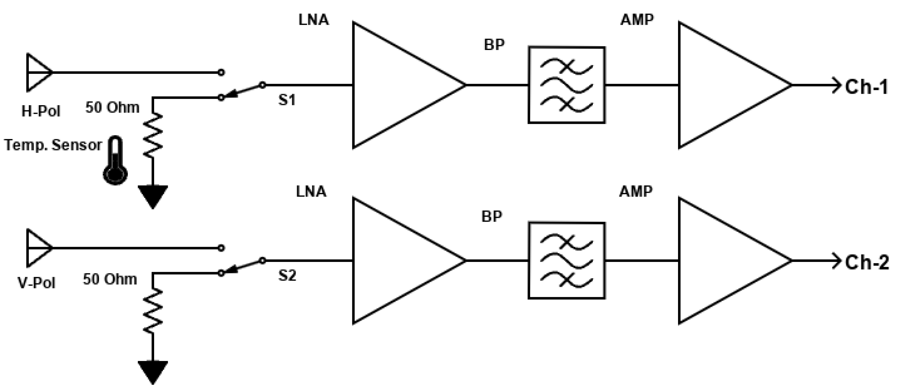
In signal order, the RF front end (Figure 1) carries a low-loss RF switch, a low-noise amplifier (LNA), a bandpass filter with a 1290–1515 MHz passband for coarse preselection, and a second-stage amplifier. The chain is replicated for each polarisation. The RF switch alternates between the antenna port and a 50-ohm reference termination every 350 ms to provide periodic calibration. This design resembles a classical Dicke receiver. However, a Dicke receiver switches fast enough to track short-term gain fluctuations; here the reference measurement instead corrects longer-term drift. The radiometer has no active temperature control, so the physical temperature of the reference load follows ambient conditions. A collocated temperature sensor records these variations every 10 s, which allows correction for the temperature-dependent noise contribution of the reference and for changes in the LNA noise figures. The LNA and second-stage amplifier together provide a small-signal power gain of 40 dB at 1405 MHz.

4.2. Digital Backend and Polarimetry

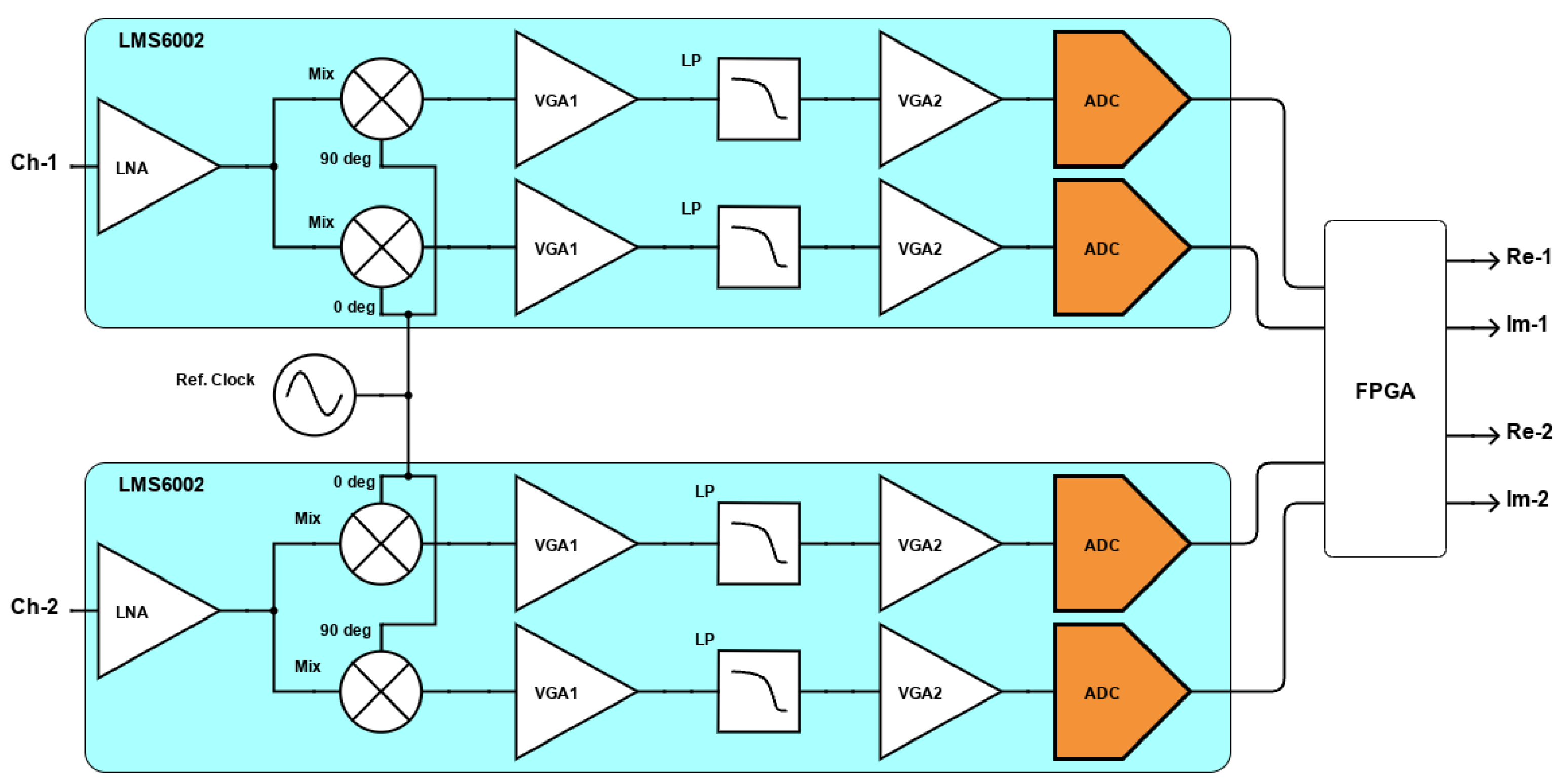
The digital backend (Figure 2) consists of a mixer for RF-to-IF downconversion, a pair of analog-to-digital converters, one per polarisation channel, and a field-programmable gate array (FPGA). The FPGA performs digital filtering, Blackman windowing, and a 256-point FFT. This channelises the band at approximately 47 kHz resolution across a 12 MHz digitised bandwidth, of which approximately 9 MHz are usable. Auto- and cross-correlation of the two polarisation channels, by complex multiplication and accumulation, yields all four Stokes parameters.

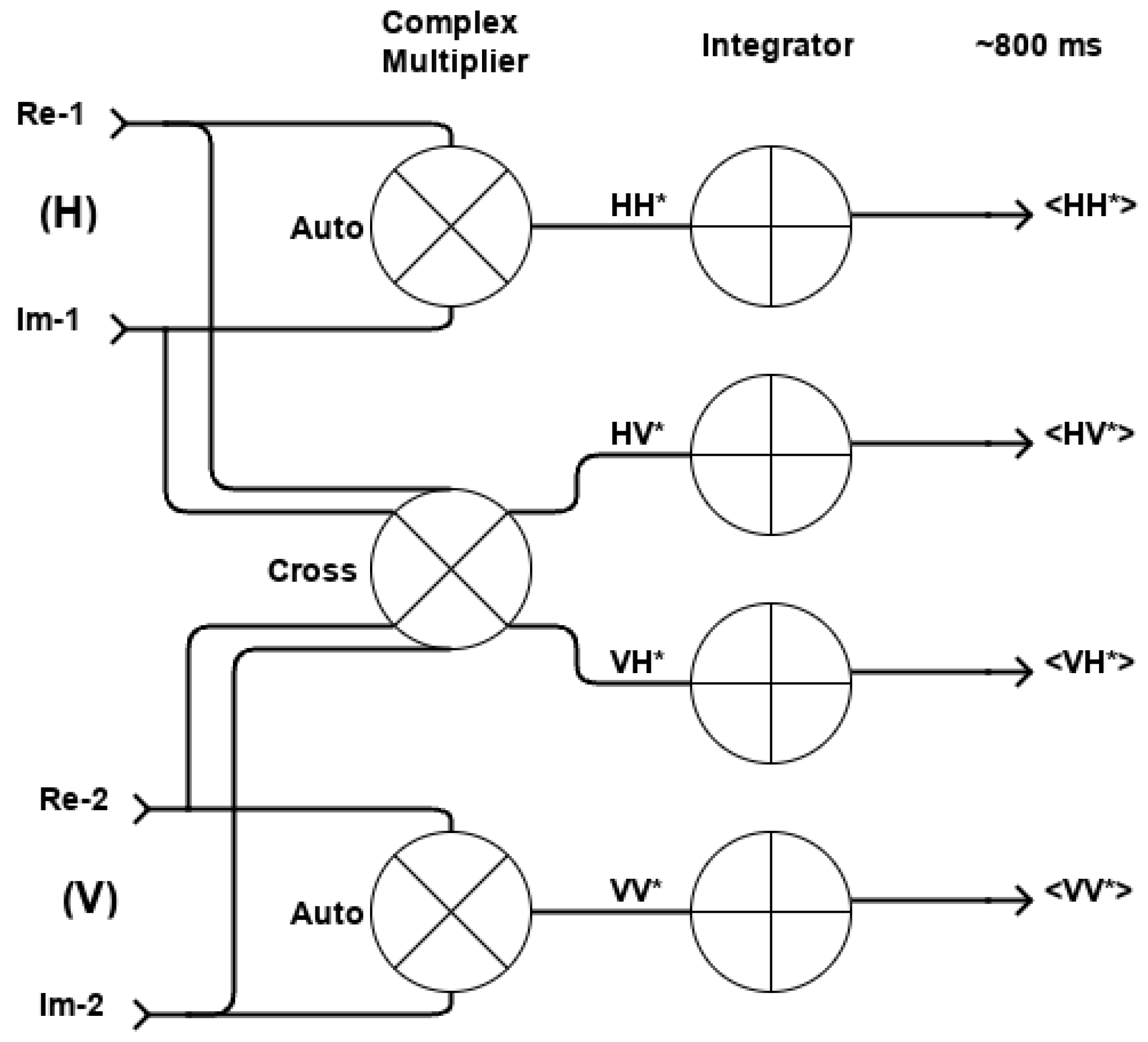
The FPGA (Figure 3) processes the digitised samples in five stages. Outlier rejection first discards frames whose sample voltages exceed dynamically adjusted thresholds based on running statistics. Each surviving 256-sample frame is then Blackman-windowed to reduce spectral leakage (equivalent noise bandwidth factor 1.73) and transformed to the frequency domain by a 256-point FFT. For every frequency bin the correlator forms the autocorrelations HH* and VV* and the complex cross-correlation HV*, resulting in the four real outputs HH*, VV*, Re(HV*), and Im(HV*). These are accumulated over 15,000 frames per cycle. The resulting integration time is approximately 700 ms per complete sample, covering both the calibration and soil measurements, and increases when frames are discarded because of RFI.

4.3. Radiometric Calibration and Sensitivity

Losses ahead of the first LNA dominate the system noise temperature. The contributing elements are antenna ohmic and mismatch losses, estimated at 0.7 dB; interconnect losses from cables and connectors, estimated at 0.3 dB; RF switch insertion loss of 0.3 dB per datasheet; and an LNA noise figure of 0.5 dB per datasheet. Each passive loss L at physical temperature $T_{\mathrm{phys}}$ contributes a noise temperature $T_{\mathrm{phys}}(L-1)$. The LNA contributes $T_{\mathrm{LNA}}=290\mathrm{K}\times ({10}^{NF/10}-1)=35\mathrm{K}$. Cascading these contributions gives a total (theoretical) system noise temperature of approximately 151 K when the RF components sit at a physical temperature of 10 °C. System noise temperature is a derived quantity, not the physical temperature of the hardware. Raising the components to a physical temperature of 50 °C raises it to 168 K: the warmer passive components contribute more noise and the LNA performance degrades. After 30 min of operation the receiver’s physical temperature typically sits near 40 °C.

We assessed the system noise temperature with a three-point calibration. For two of the points the antenna was replaced by a 75 cm-long cable, whose 0.6 dB measured loss approximates the antenna path loss, terminated in 50-ohm loads at controlled temperatures: a cold load at $-20 °$C (253 K) and a hot load at $+110 °$C (383 K). The third point used the complete system viewing the zenith sky. The L-band sky brightness temperature is approximately 5–8 K from the cosmic and galactic background, and sidelobe contributions raise the effective antenna temperature to approximately 10 K. The radiometer outputs were 262 K for the cold load, 355 K for the hot load, and 131 K for the cold sky. Linear regression gave an offset of 122 K and a gain correction factor of 1.69. The estimated system noise temperature is therefore 206 K, which is above the theoretical estimate derived in the previous paragraph. We attribute the difference to additional losses not captured in the component-level analysis and to uncertainties in the published component data sheets. An additional 0.5 to 1 dB of loss ahead of the LNA, within the tolerance of the datasheet figures, would raise the predicted system noise temperature by roughly 30 to 60 K and account for most of the gap.

The noise-equivalent delta temperature (NE$\Delta$T) characterises radiometric sensitivity, the minimum detectable change in brightness temperature over a single integration period. For a single polarisation channel,

$$\mathrm{NE}\Delta {\mathrm{T}}_{\mathrm{pol}}={\displaystyle \frac{T_{\mathrm{sys}}}{\sqrt{B_{\mathrm{eff}}\tau }}}$$

(1)

where $T_{\mathrm{sys}}$ is the system noise temperature, $B_{\mathrm{eff}}$ is the effective noise bandwidth, and $\tau$ is the integration time. The RF analog bandwidth is approximately 9 MHz. With the Blackman window equivalent noise bandwidth factor of 1.73, the effective bandwidth is $B_{\mathrm{eff}}\approx 5.2$ MHz. The system alternates between the antenna and the calibration load with 350 ms per state, so the effective integration time per antenna measurement is $\tau =0.35$ s.

We measured the single-polarisation sensitivity by observing the internal calibration load at physical temperature $T_{\mathrm{ref}}\approx 300$ K, over a 400 s period. Viewing a warm target, the effective system temperature is $T_{\mathrm{sys}}+T_{\mathrm{ref}}=506$ K, giving a theoretical sensitivity of 0.38 K.

After subtracting a fitted polynomial baseline to remove slow instrumental drifts, the measured standard deviation was 0.42 K, in good agreement with theory. The small difference falls within the combined uncertainties of the system noise temperature measurement, the reference load temperature, and the effective bandwidth estimate. A sensitivity of 0.42 K corresponds to a single-measurement VWC noise of approximately 0.4% VWC, given the $T_{\mathrm{B}}$-to-VWC calibration slope described in Section 6. This is well below the random error, so instrument noise is not the limiting factor. The dominant error contributions are calibration uncertainty and the mismatch between the sensor footprint and the point measurements used as reference.

4.4. Sensor Integration and Data Collection

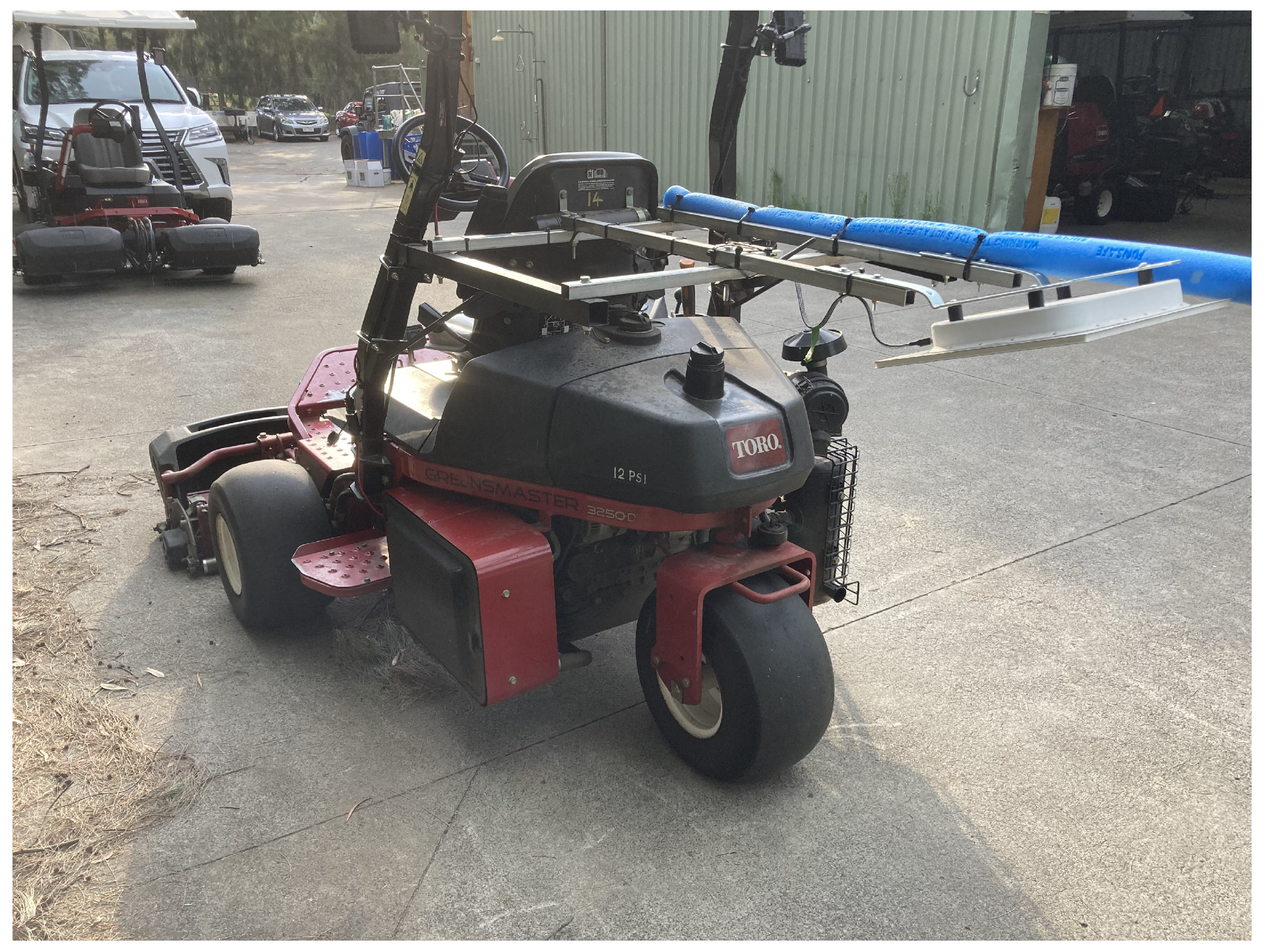
The sensor is mounted approximately 1.2 m above the ground (Figure 4). The mount results in an off-nadir viewing angle of approximately 15°, which shifts the footprint clear of the mower body. The small polarisation effect at this incidence angle is neglected, and we treat the measurement geometry as nadir. At this height the 34° half-power beamwidth produces a near-circular footprint approximately 75 cm in diameter.

Microwave data were collected during regular mowing sessions between 23 November 2025 and 15 January 2026, giving approximately 16 sessions per green across the five greens. Each green was mapped in a single mowing pass of several minutes, yielding approximately 350–460 measurements per green per session at a rate of about one measurement every 0.7 to 1 s. The sensor’s built-in GNSS module georeferences each measurement, with a typical horizontal accuracy of 2–3 m.

4.5. Ground-Truth Validation Measurements

At the time of this study no permanently installed soil moisture sensors were in place on the greens. Handheld dielectric probes were used for periodic spot checks, but no spatially continuous soil moisture data were available. About 20 ground-truth measurements were collected per green, taken alongside the microwave radiometer data on 13 January 2026 between approximately 08:30 and 09:45 local time. The validation maps (Section 7.2) are from the mowing pass made during this window: Green 10 at 08:34, Green 17 at 08:50, Green 16 at 09:18, Green 11 at 09:28, and Green 13 at 09:42 local. The probe readings were taken during the same pass, so the microwave and probe measurements for each green are simultaneous. At each location we recorded two independent handheld probes inserted between 0.2 and 0.5 m apart: a Pogo mobile soil moisture probe and a FieldScout TDR 350. At this spacing the metal rods of one probe do not interfere electromagnetically with the other probe’s reading, and the two probes still sample the same general soil condition. We chose the validation points deliberately rather than at random. The sampling targeted topographic extremes, such as elevated ridges and low-lying areas, together with locations typical of the wider green surface. Small-scale moisture anomalies were avoided in favour of the general moisture trends.

The Pogo TurfPro Plus mobile soil moisture probe (Stevens Water Monitoring Systems, Inc., Portland, OR, USA) uses a Stevens HydraProbe II sensor based on coaxial impedance dielectric reflectometry (referred to as HydraProbe hereafter). The sensor measures volumetric water content by a method validated by [28], who reported a mean error of 1.9% VWC for the general calibration. The probe’s 5.6 cm metal rods measure to a depth of approximately 6 cm. The FieldScout TDR 350 (Spectrum Technologies, Inc., Aurora, IL, USA) is a time-domain-reflectometry probe fitted here with 3.8 cm rods, applying a calibration distinct from the HydraProbe’s dielectric model and sensing a slightly shallower layer. The FieldScout TDR 350 serves as the primary reference for the validation statistics below; the HydraProbe is a second co-located probe, used to quantify the representativeness error referred to in Section 8.

5. Microwave Data Processing

Each microwave sensor integration yields six spectra of 256 channels. Two spectra measure power in the H and V channels of the calibration noise source (the cross-correlation products are not needed for internal calibration). The other four capture the soil signal, namely the two autocorrelations HH* and VV* and the real and imaginary parts of the complex cross-correlation HV*. The same processing chain runs on all data, regardless of field or sensor, and no step is performed by hand.

Raw data are first flagged for outliers, excessive radio interference, and occasional instrument glitches. Amplitude thresholds reject anomalous calibration signals and excise individual spectral channels. A reference bandpass response is then derived from the calibration noise source measurements, with RFI-contaminated channels excluded. Dividing every spectrum by this bandpass corrects for the frequency-dependent system response.

The antenna correlation products (ant), which contain the soil signal, are normalised against the corresponding calibration signal from the 50-Ohm termination (ref) and scaled by the physical temperature ($T_{\mathrm{phys}}$) of the calibration source:

$${\mathrm{HH}}^{\prime }\left(K\right)=T_{\mathrm{phys}}·{\displaystyle \frac{{\mathrm{HH}}_{\mathrm{ant}}^{\ast }}{{\mathrm{HH}}_{\mathrm{ref}}^{\ast }}}$$

(2)

with an analogous expression for VV. The 50-Ohm reference terminations emit uncorrelated noise on the H and V outputs, so ${\mathrm{HV}}_{\mathrm{ref}}^{\ast }\approx 0$ and cannot serve as a reference for the cross-correlation product. Because ${\mathrm{HV}}^{\ast }$ scales as $\sqrt{g_H{g}_V}$ rather than as either channel’s own gain, it is instead normalised against the geometric mean of the two reference auto-spectra:

$${\mathrm{HV}}^{\prime }\left(K\right)=T_{\mathrm{phys}}·{\displaystyle \frac{{\mathrm{HV}}_{\mathrm{ant}}^{\ast }}{\sqrt{{\mathrm{HH}}_{\mathrm{ref}}^{\ast }·{\mathrm{VV}}_{\mathrm{ref}}^{\ast }}}}.$$

(3)

This normalisation puts the products on a provisional temperature scale, but two corrections remain before they give a soil brightness temperature. Receiver noise varies with the physical temperature of the electronics, so we subtract an empirically fitted drift term:

$$\Delta T_{\mathrm{HH}}=T_{\mathrm{phys}}(°\mathrm{C})·\left(a_{\mathrm{HH}}·{\mathrm{HH}}^{\prime }+b_{\mathrm{HH}}\right),T_{\mathrm{corr},\mathrm{HH}}={\mathrm{HH}}^{\prime }-\Delta T_{\mathrm{HH}}.$$

(4)

The gain $g_{\mathrm{HH}}$ and offset $c_{\mathrm{HH}}$ from the three-point calibration (Section 4.3) then place this on the absolute Kelvin scale:

$$T_{\mathrm{soil},\mathrm{HH}}=g_{\mathrm{HH}}·T_{\mathrm{corr},\mathrm{HH}}+c_{\mathrm{HH}}.$$

(5)

The VV channel is processed identically with its own coefficients.

Using these calibrated brightness temperatures, the four Stokes parameters follow as

$$\begin{array}{cccc}\hfill I& =\frac{1}{2}(T_{\mathrm{HH}}+T_{\mathrm{VV}}),\hfill & \hfill Q& =\frac{1}{2}(T_{\mathrm{HH}}-T_{\mathrm{VV}}),\hfill \\ \hfill U& =\mathrm{Re}\left(T_{\mathrm{HV}}\right),\hfill & \hfill V& =\mathrm{Im}\left(T_{\mathrm{HV}}\right).\hfill \end{array}$$

(6)

These follow the standard radiometric Stokes formalism [22], so that I equals the single-channel brightness temperature an unpolarised target would produce. We assume the H and V receiver chains are phase-stable and apply no separate calibration for their relative phase. An uncalibrated phase offset between the two chains would rotate power between U and V, but leaves $\sqrt{U^2+V^2}$, and hence the polarised and interference estimates below, unchanged.

The polarised and unpolarised components of the brightness temperature are then

$$T_{\mathrm{pol}}=\sqrt{Q^2+U^2+V^2},T_{\mathrm{unpol}}=I-T_{\mathrm{pol}}.$$

(7)

Radio interference is predominantly polarised, whereas soil emission is nearly unpolarised at the incidence angles used here, so we subtract a weighted estimate of the interference from the total intensity:

$$T_{\mathrm{RFI}}=\sqrt{{\left(w_{U}U\right)}^2+{\left(w_{Q}Q\right)}^2+{\left(w_{V}V\right)}^2}$$

(8)

in which $w_U$, $w_Q$, and $w_V$ are empirical coefficients. Hence, $T_{\mathrm{RFI}}$ is an estimate of the interference contribution to the total intensity, not a polarised brightness temperature in the strict sense, and $T_{\mathrm{clean}}=I-T_{\mathrm{RFI}}$ is the corrected signal.

The weights are determined once per green on the accumulated maps and are chosen to minimise the brightness-temperature difference between maps from consecutive sessions. On greens without detectable interference the fit returns zero and nothing is subtracted. On the affected greens the fit returns non-zero weights; on the most strongly affected greens (1–4), $w_U$ and $w_V$ fall in the range 20–40 while $w_Q$ remains below 1. The technical or physical origin of the weights is unknown.

The spectrum for each integration is then collapsed to a single value by taking the median across all unflagged channels, yielding one brightness temperature ($T_{\mathrm{clean}}$) per measurement location.

A further safeguard catches instrument faults and transient interference. A session whose brightness-temperature statistics depart sharply from the recent history of a green is withheld, so a faulty or strongly interfered measurement set cannot corrupt the accumulated distribution.

On the survey day, 13 January 2026, this safeguard flagged an instrument offset of roughly 10–20 K on all five validation greens. It corrected the offset using each green’s existing baseline, so the flagged session neither altered that baseline nor affected the sessions around it.

6. Automated Per-Green Calibration

Absolute calibration (the conversion of $T_{\mathrm{B}}$ to absolute VWC) is automated by a deliberately simplistic scheme. We assume a linear relation between brightness temperature and volumetric water content, so the conversion needs only two fitted parameters, a slope and an offset, together with the assumed range between two calibration anchors at the dry and wet ends. The slope $a_{\mathrm{std}}=-1/{\sigma }_{T_{\mathrm{B}}}$ depends only on the width ${\sigma }_{T_{\mathrm{B}}}$ of the long-term $T_{\mathrm{B}}$ distribution and maps $T_{\mathrm{B}}$ onto a dimensionless score. It is negative because wetter soil emits at lower $T_{\mathrm{B}}$. Because it depends only on ${\sigma }_{T_{\mathrm{B}}}$, this slope is a sensor property, characterised once per sensor from data across all greens and then held fixed. ${\sigma }_{T_{\mathrm{B}}}$ itself is not measured on a single green or session. Any one session reflects that green’s own irrigation, soil, and canopy state at that moment, so the estimate is instead pooled across many greens and sessions, and locked once its variation falls below a fixed threshold. Green-to-green and session-to-session variability thus averages out rather than propagating into the slope. The offset $b_{\mathrm{std}}$, on the other hand, is specific to each green, because each green sits in a distinct local radio frequency interference (RFI) environment. The dimensionless score is converted to absolute VWC using the two calibration anchors ${\theta }_{\mathrm{dry}}$ and ${\theta }_{\mathrm{wet}}$, as described below.

The per-green $T_{\mathrm{B}}$-to-VWC mapping is built up by accumulating mowing passes over time (

Table 1. Calibration framework.

Measured Data
1. $T_{\mathrm{B}}$ (K) from mower-mounted radiometer
2. Multiple sessions per green over time
Required Inputs
1. Initial calibration anchors ${\theta }_{\mathrm{dry}}$ and ${\theta }_{\mathrm{wet}}$, ideally from soil tables, a dielectric probe, or gravimetric sampling. Informed estimates are also valid, provided they are close to correct on average across the whole course
2. Management: irrigation maintains moisture within the ${\theta }_{\mathrm{dry}}$–${\theta }_{\mathrm{wet}}$ range
Core Assumptions
1. Calibration slope $a_{\mathrm{std}}$ is stable after sufficient characterisation sessions.
2. The dry anchor ${\theta }_{\mathrm{dry}}$ changes negligibly over multi-year timescales; the high anchor ${\theta }_{\mathrm{wet}}$ varies slowly with thatch and rootzone condition
3. Ambient radio interference at each green is approximately stable over a rolling window timescale.
4. Greens irrigated to a consistent moisture range within the available water.
5. Target VWC distribution is approximately Gaussian over the operating range
6. $T_{\mathrm{B}}$–VWC relationship is linear with a negative slope (wet → low $T_{\mathrm{B}}$, dry → high $T_{\mathrm{B}}$)

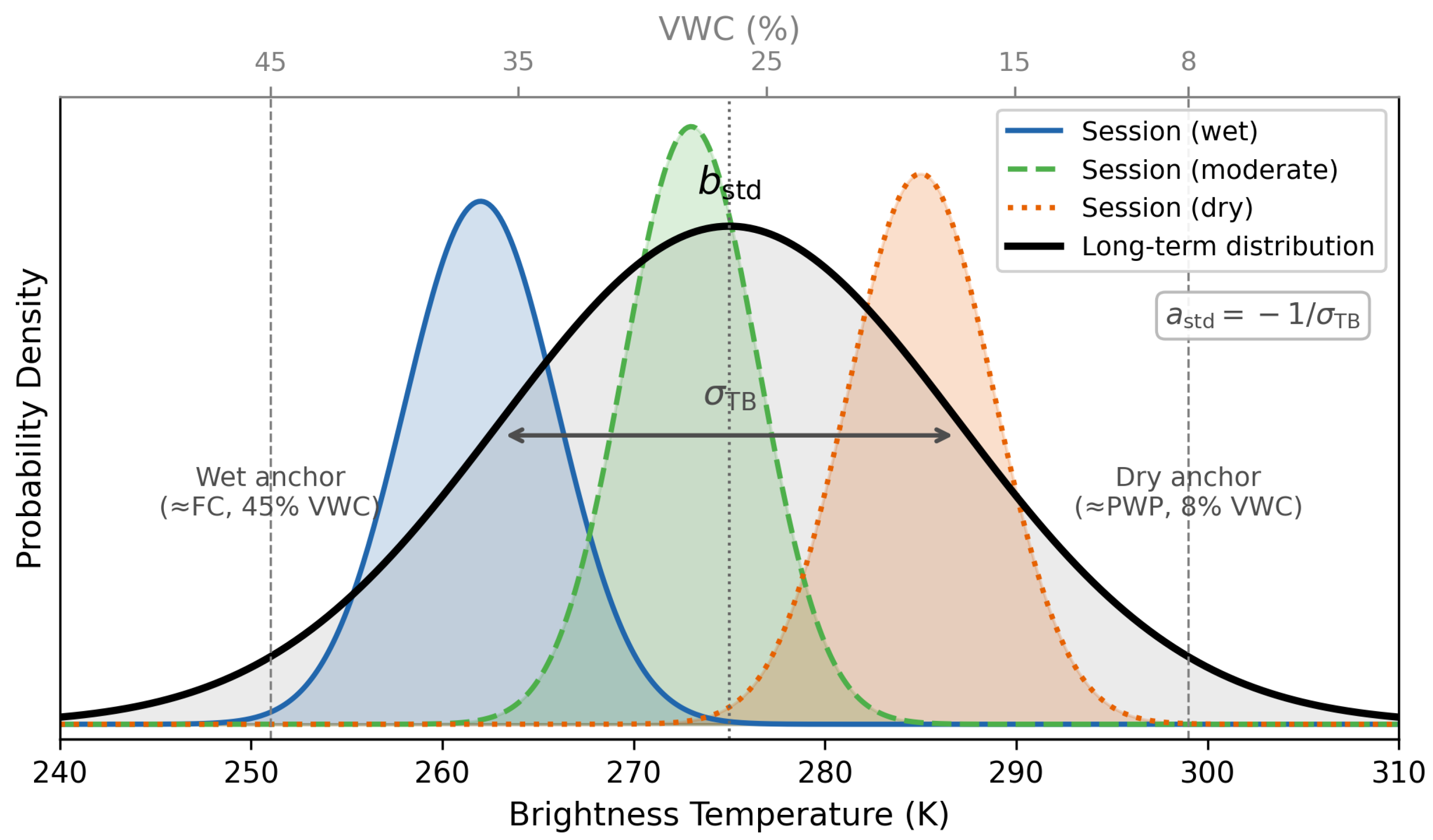
). Each pass across a green is one session and produces hundreds of $T_{\mathrm{B}}$ measurements, capturing the spatial moisture distribution at that moment. However, a single session samples only a narrow range of moisture values. For example, a session after a dry weekend produces a $T_{\mathrm{B}}$ distribution at the dry end. A session in the morning after rain produces one at the wet end. No single session spans the full range between permanent wilting point and field capacity.

Collected under varying conditions over many sessions, the narrow session distributions build up a wide long-term $T_{\mathrm{B}}$ distribution that spans the moisture range the green can hold (Figure 5). The ends of this distribution line up with the hydraulic limits because (a) management does not let the soil dry much past the wilting point, so the dry end of the distribution sits near that limit, and (b) water added beyond field capacity drains within hours, so the soil cannot stay wetter for long and the wet end sits near field capacity. We define calibration anchors ${\theta }_{\mathrm{dry}}$ and ${\theta }_{\mathrm{wet}}$ at these ends, which is an approximate correspondence since managers irrigate before true wilting and the soil briefly exceeds field capacity after watering.

The algorithm maps this long-term distribution onto the expected VWC distribution. Each new session extends the observed $T_{\mathrm{B}}$ range, so the slope settles as sessions accumulate. In operational deployment, $b_{\mathrm{std}}$ is the median over a rolling multi-season window; for the eight-week dataset reported here, it was computed from all available sessions.

With both parameters established, the algorithm converts $T_{\mathrm{B}}$ to VWC. The initial values ${\theta }_{\mathrm{dry}}=8\%$ and ${\theta }_{\mathrm{wet}}=45\%$ come from the superintendent’s experience managing these greens. They are informal estimates, not probe measurements and not the result of a soil survey. The 45% value sits well above the field capacity expected for USGA sand rootzones [26]. It reflects the thatch and organic matter in the upper few centimetres of these greens, which holds more water than the sand below; the probes and the radiometer both sense that layer preferentially. The anchors are calibration parameters, not independently measured hydraulic limits, and their relation to the rootzone’s true field capacity is left open here.

The equation that implements the mapping is

$$\mathrm{VWC}={\mathrm{VWC}}_{\mathrm{cen}}+{\sigma }_{\mathrm{VWC},\mathrm{target}}{a}_{\mathrm{std}}(T_{\mathrm{B}}-b_{\mathrm{std}}),$$

(9)

where $a_{\mathrm{std}}=-1/{\sigma }_{T_{\mathrm{B}}}$ and $b_{\mathrm{std}}$ are as defined above. The equation works in two steps. The term $a_{\mathrm{std}}(T_{\mathrm{B}}-b_{\mathrm{std}})$ centres and scales the $T_{\mathrm{B}}$ reading to a dimensionless score: how far the measurement sits from the long-term mean, normalised by the distribution width. Then ${\mathrm{VWC}}_{\mathrm{cen}}=({\theta }_{\mathrm{wet}}+{\theta }_{\mathrm{dry}})/2$ and ${\sigma }_{\mathrm{VWC},\mathrm{target}}=0.40({\theta }_{\mathrm{wet}}-{\theta }_{\mathrm{dry}})$ rescale that score to absolute VWC, placing ${\theta }_{\mathrm{dry}}$ and ${\theta }_{\mathrm{wet}}$ at $\pm 1.25{\sigma }_{\mathrm{VWC},\mathrm{target}}$. The first step is a sensor property, fixed once enough sessions have accumulated; the second is set by ${\theta }_{\mathrm{dry}}$ and ${\theta }_{\mathrm{wet}}$. When ${\theta }_{\mathrm{wet}}$ is updated through adaptive refinement, ${\mathrm{VWC}}_{\mathrm{cen}}$ and ${\sigma }_{\mathrm{VWC},\mathrm{target}}$ shift with it, but $a_{\mathrm{std}}$ does not.

The high anchor is refined over time. The wet-end percentile of the accumulated $T_{\mathrm{B}}$ distribution, near the 98th percentile of VWC, gives a running estimate of the wet end, and when it drifts from the current anchor the high anchor is nudged toward it. The low (dry) anchor is held fixed to prevent unbounded drift. This fine-tuning works because $a_{\mathrm{std}}$ is locked before any anchor adjustment, and the high anchor is tracked against the stable $T_{\mathrm{B}}$ percentiles rather than against the converted VWC, so the refinement cannot feed back into the slope. The high anchor is treated as slowly varying: as thatch and organic matter change the water held in the sensed surface layer, the wet end of the distribution shifts over multi-year timescales.

Self-calibrating L-band retrievals have precedent. Peng et al. [29] proposed a parameter self-calibrating framework for a multi-channel SMAP algorithm that solves for surface roughness and scattering albedo internally, without auxiliary vegetation or soil moisture data. Our scheme also calibrates from the data themselves, but in a different way. Rather than solving for physical parameters, it anchors the accumulated brightness-temperature distribution onto a fixed VWC range, requiring no field calibration of the absolute scale. This distribution anchoring also differs from quantile matching, which maps onto a reference distribution rather than fixed endpoints.

A physical Tau–Omega retrieval is the natural alternative. Houtz et al. used one for turf, with a single canopy parameter justified by the uniform fairway grass [9]. The close-mown canopy here contributes negligible attenuation, so such a retrieval would be nearly free of vegetation parameters. The real constraint lies elsewhere. Tau–Omega inverts the absolute brightness temperature and carries no term for radio interference; it therefore needs accurate absolute calibration and assumes interference is absent or removed beforehand. On a moving instrument that crosses greens, each in a different and uncharacterised local interference environment, meeting that requirement per green is impractical. The present scheme is probably better suited for such an environment. It tolerates a constant per-green interference offset and leaves the polarimetric subtraction to handle the time-varying part, at the cost of an absolute scale fixed by the anchors rather than by absolute calibration.

The system cannot recover absolute VWC values from a single session. It anchors the calibration to the initial estimates ${\theta }_{\mathrm{dry}}$ and ${\theta }_{\mathrm{wet}}$ and to the assumption that irrigation holds soil moisture within a consistent target range. If those estimates are wrong, or if irrigation is inconsistent, the whole VWC scale shifts with them. Refining the high anchor may pull it back over time, but we have not tested that, so we treat the absolute scale as provisional. The calibration further assumes that the RFI environment at each green is approximately stable over the rolling window; what happens when this assumption fails is discussed in Section 8.

Because $a_{\mathrm{std}}$ is a property of the sensor, the brightness-temperature-to-VWC slope is common to all greens:

$$\mathrm{VWC}[\%]=-1.04[\%{\mathrm{K}}^{-1}]\left(T_{\mathrm{B}}-T_{\mathrm{B}0}\right),$$

(10)

with $-1.04\%{\mathrm{K}}^{-1}={\sigma }_{\mathrm{VWC},\mathrm{target}}{a}_{\mathrm{std}}$ and $a_{\mathrm{std}}=-1/{\sigma }_{T_{\mathrm{B}}}=-0.070{\mathrm{K}}^{-1}$ (${\sigma }_{T_{\mathrm{B}}}=14.3$ K). Only the offset $T_{\mathrm{B}0}$ varies between greens (

Table 2. Per-green offset for the conversion of Equation (10). The sensor factor $-1.04\%{\mathrm{K}}^{-1}$ is common to all greens; only $T_{\mathrm{B}0}$, the brightness temperature at which the retrieval returns VWC $=0$, differs. $T_{\mathrm{B}0}$ contains contributions from the instrument noise, soil emission, and the local RFI environment.

Green	${\mathit{T}}_{\mathbf{B}0}$ (K)
10	280.6
11	280.9
13	281.7
16	282.5
17	283.2

).

7. Results

7.1. Spatial Moisture Patterns and Temporal Consistency

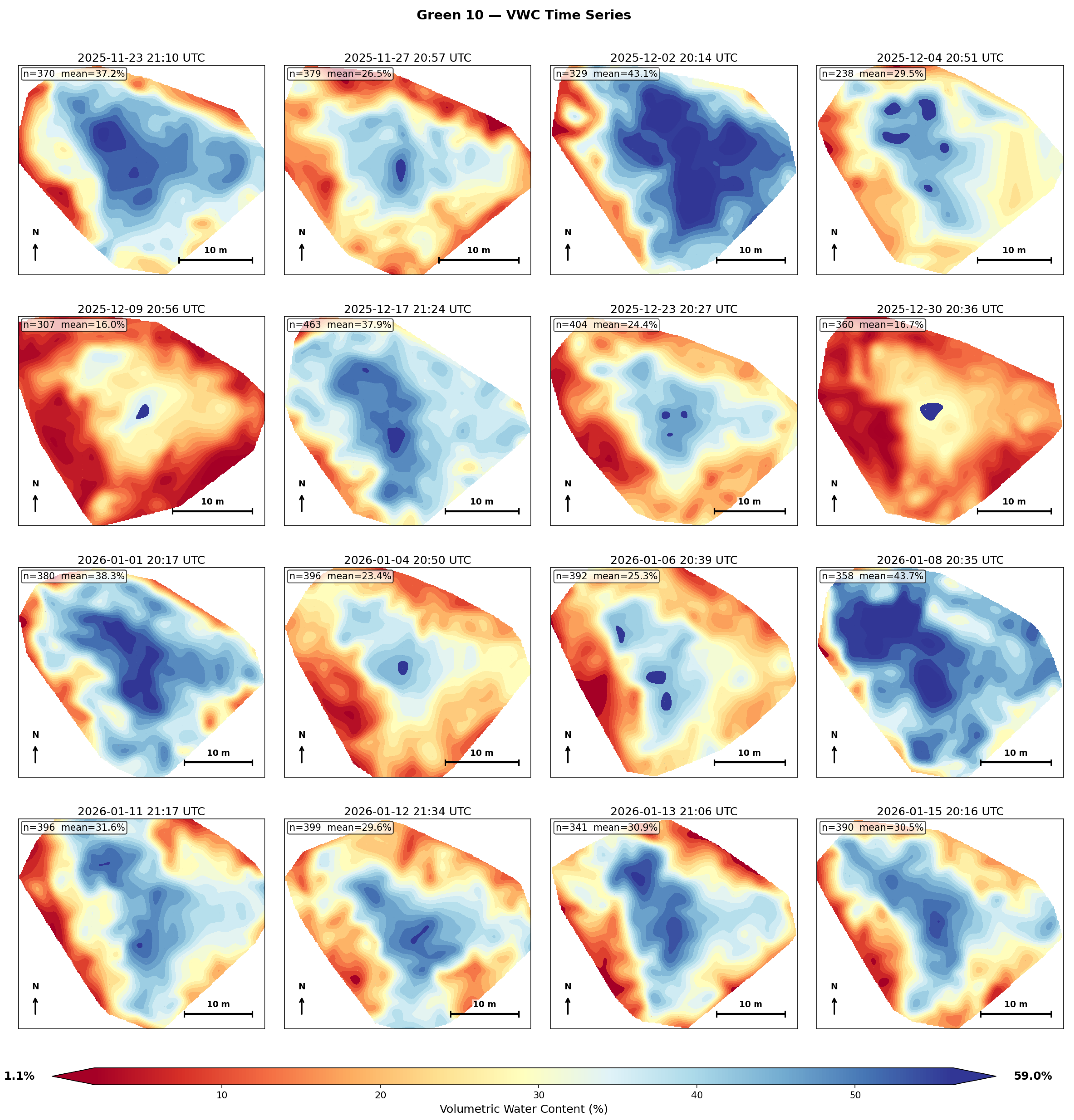
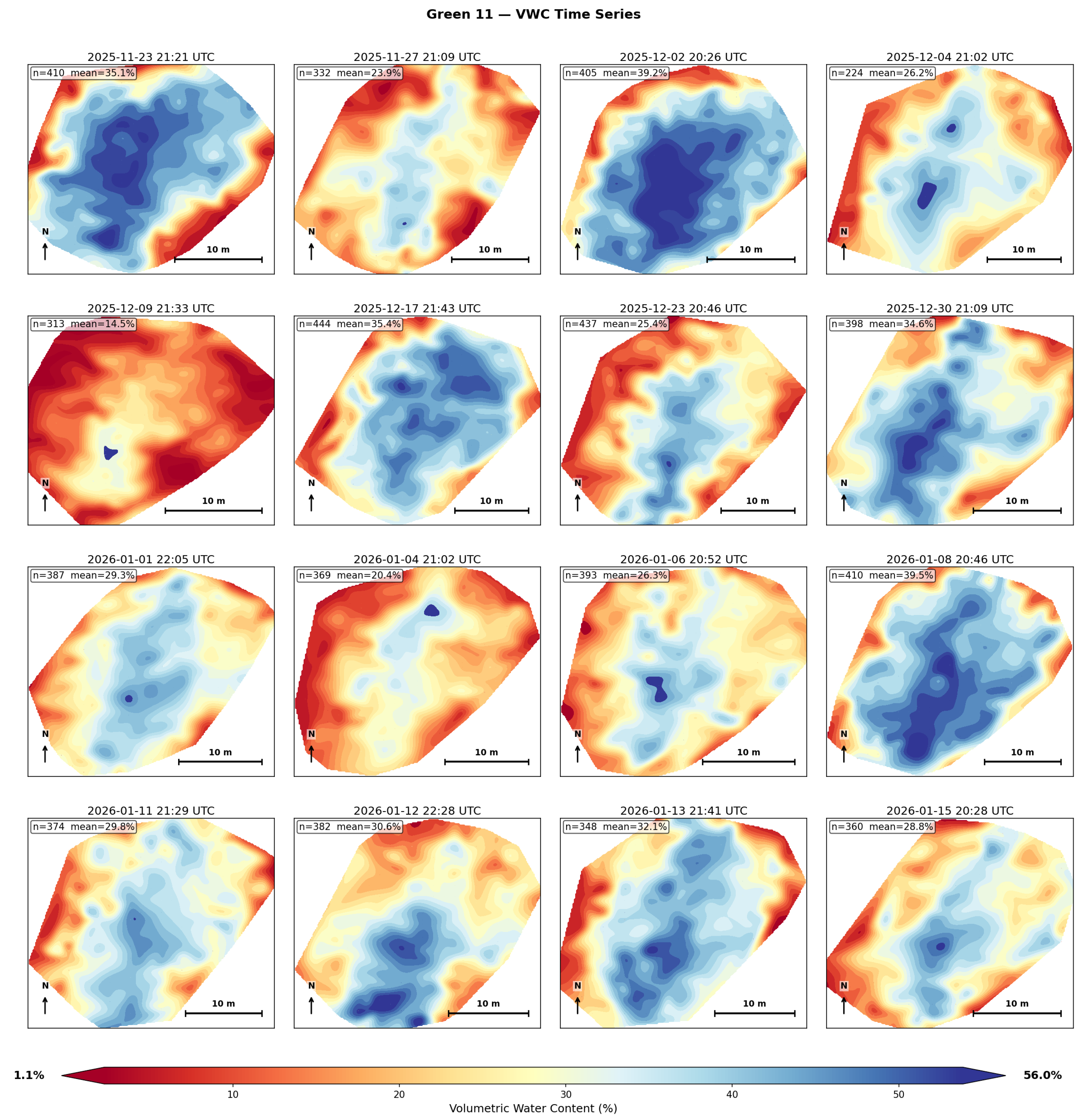
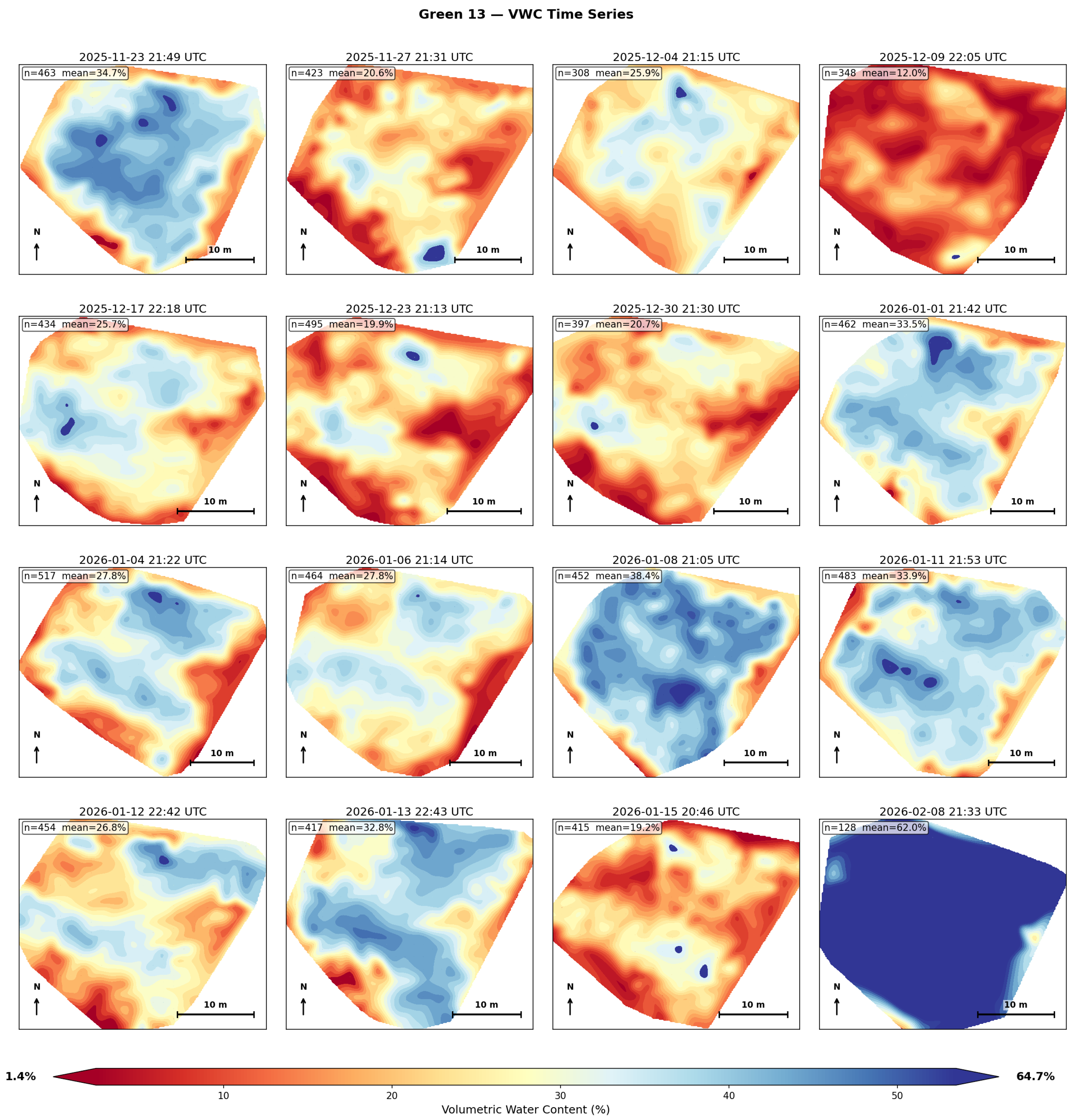
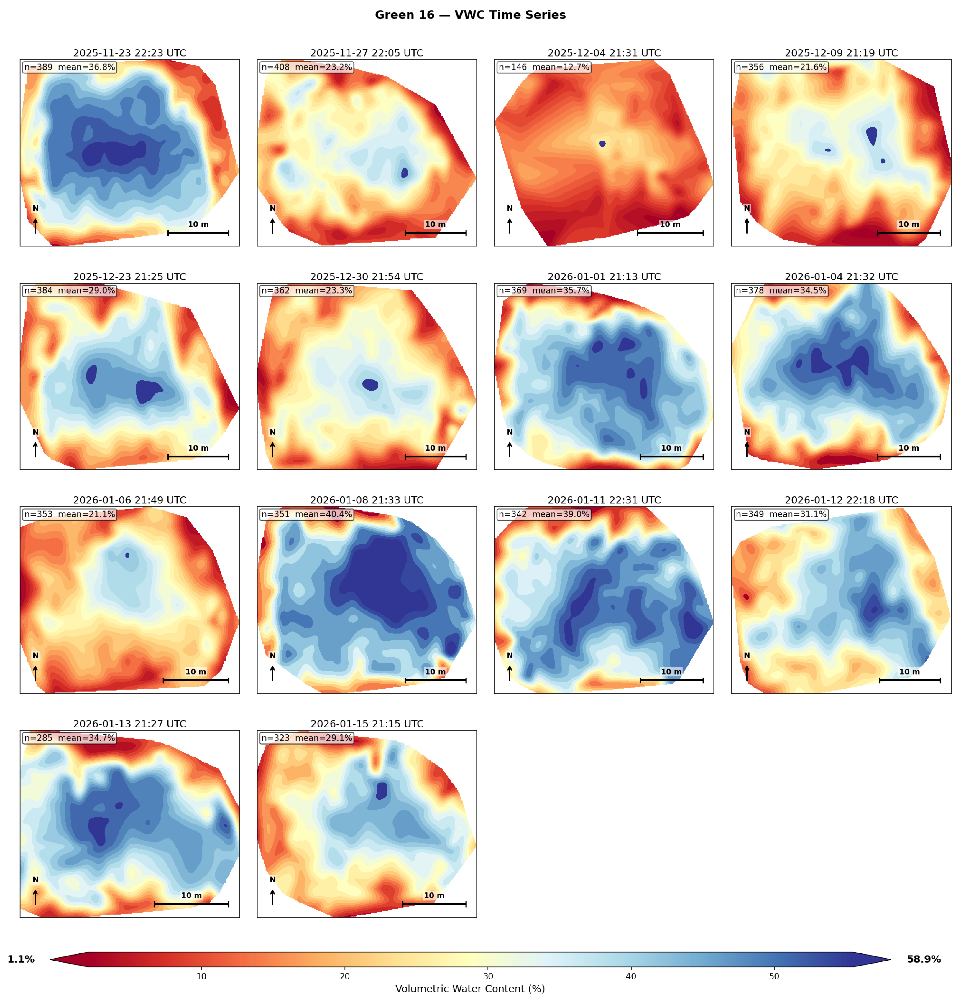
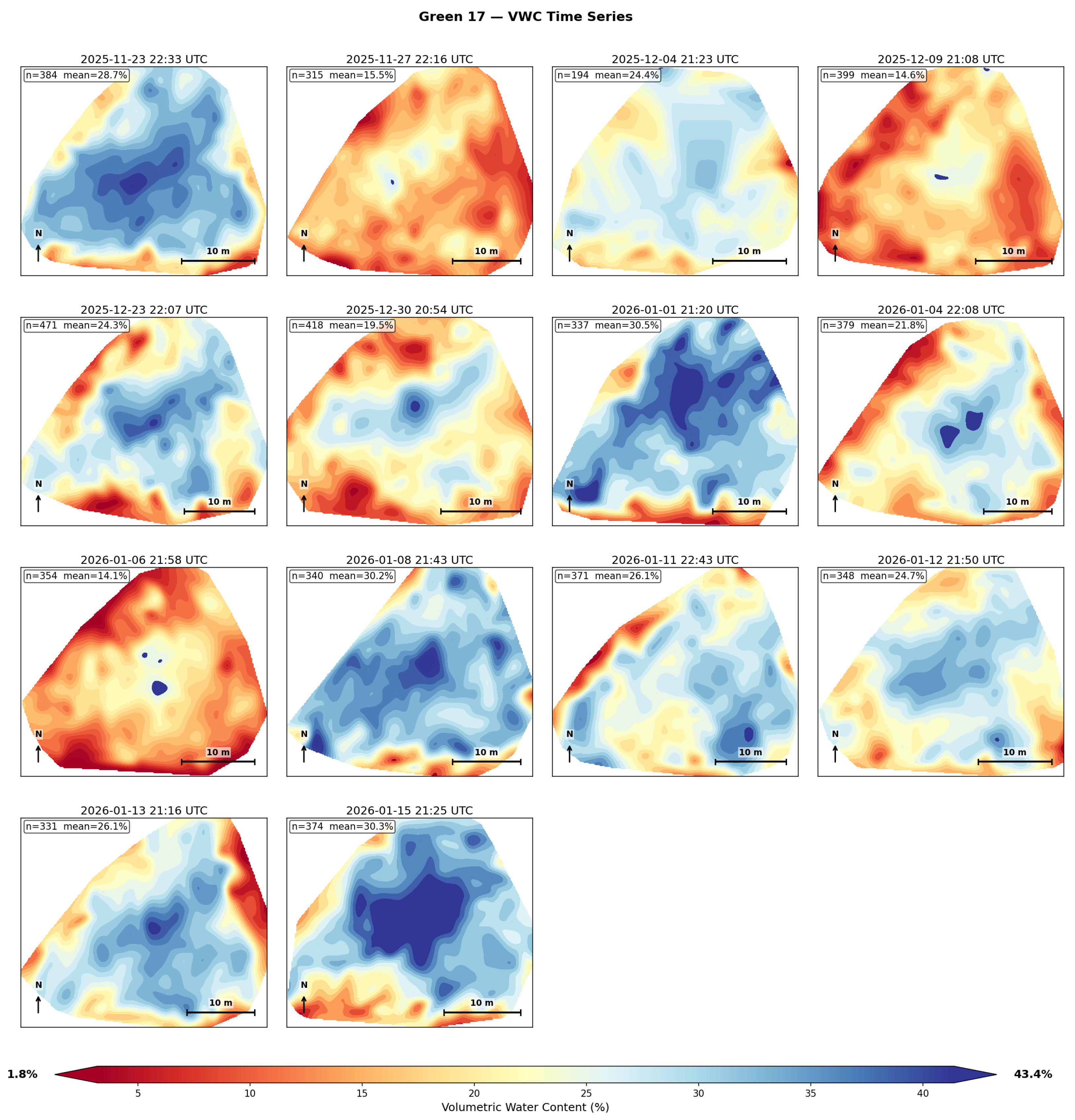
Figure 6, Figure 7, Figure 8, Figure 9 and Figure 10 show VWC maps for all mowing sessions on each green. Wet and dry zones persist at the same locations from session to session, across the full observation period. The instrument is therefore detecting real structure in the soil moisture distribution, not measurement noise.

The pattern are stable in their position while the overall moisture level of each green rises and falls with irrigation and weather, which points to fixed properties of the green as their cause. The structure within a green likely is due to the sensing depth: surface microrelief and the drainage it controls, localised water repellency, and the differences in thatch, organic matter, and compaction that were not characterised here. Elevation and rootzone properties were not surveyed, so the maps display this variability rather than explain its cause.

7.2. Validation

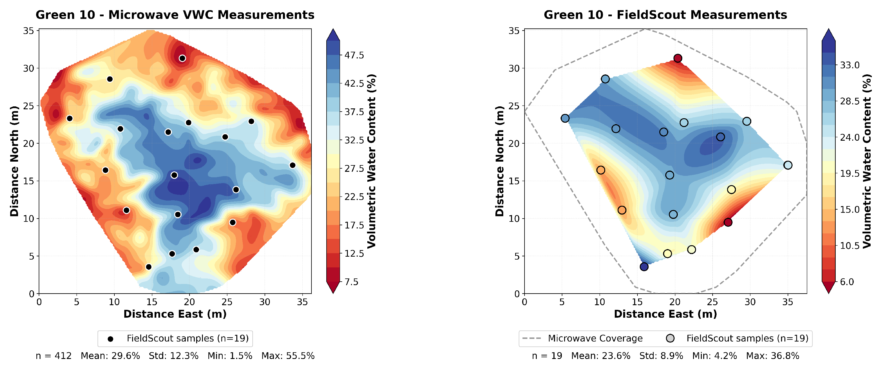
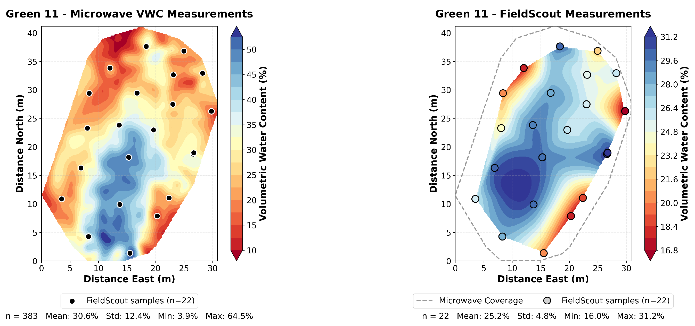
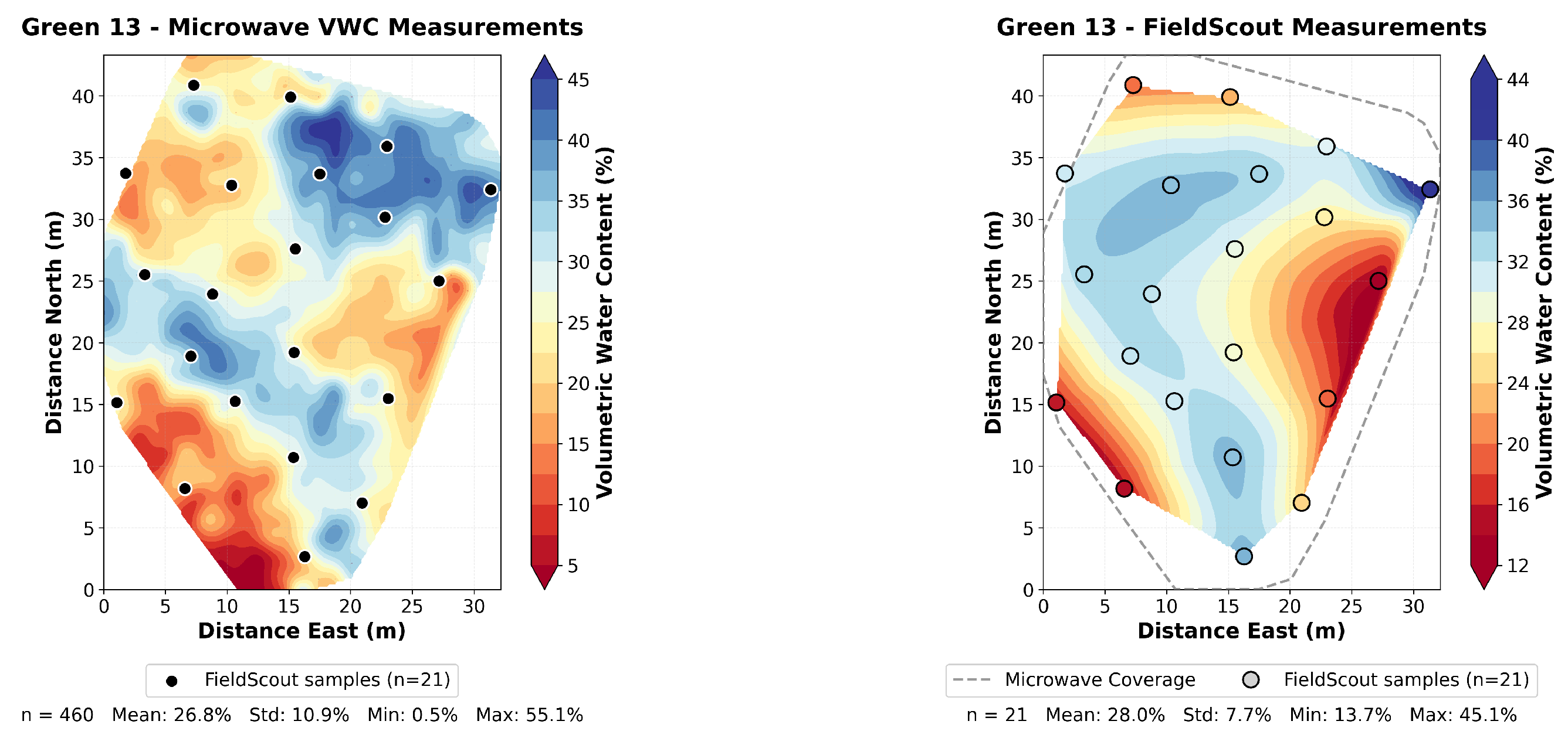
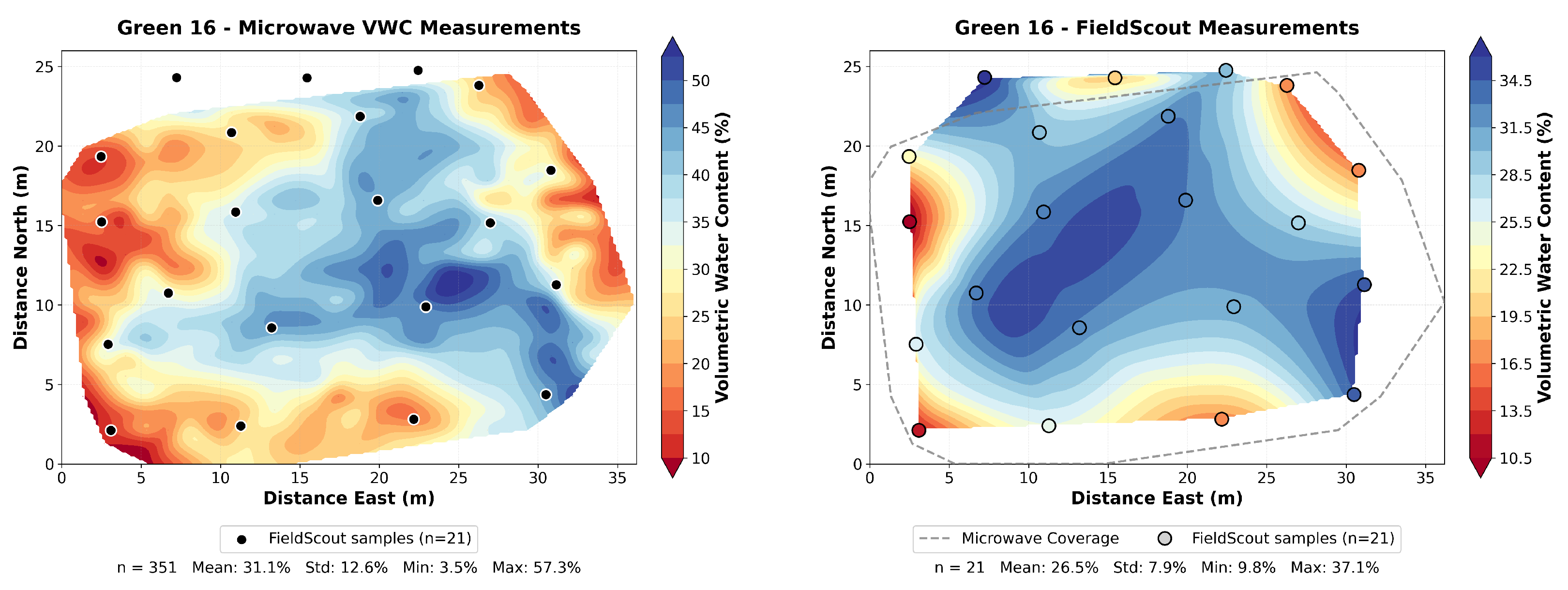
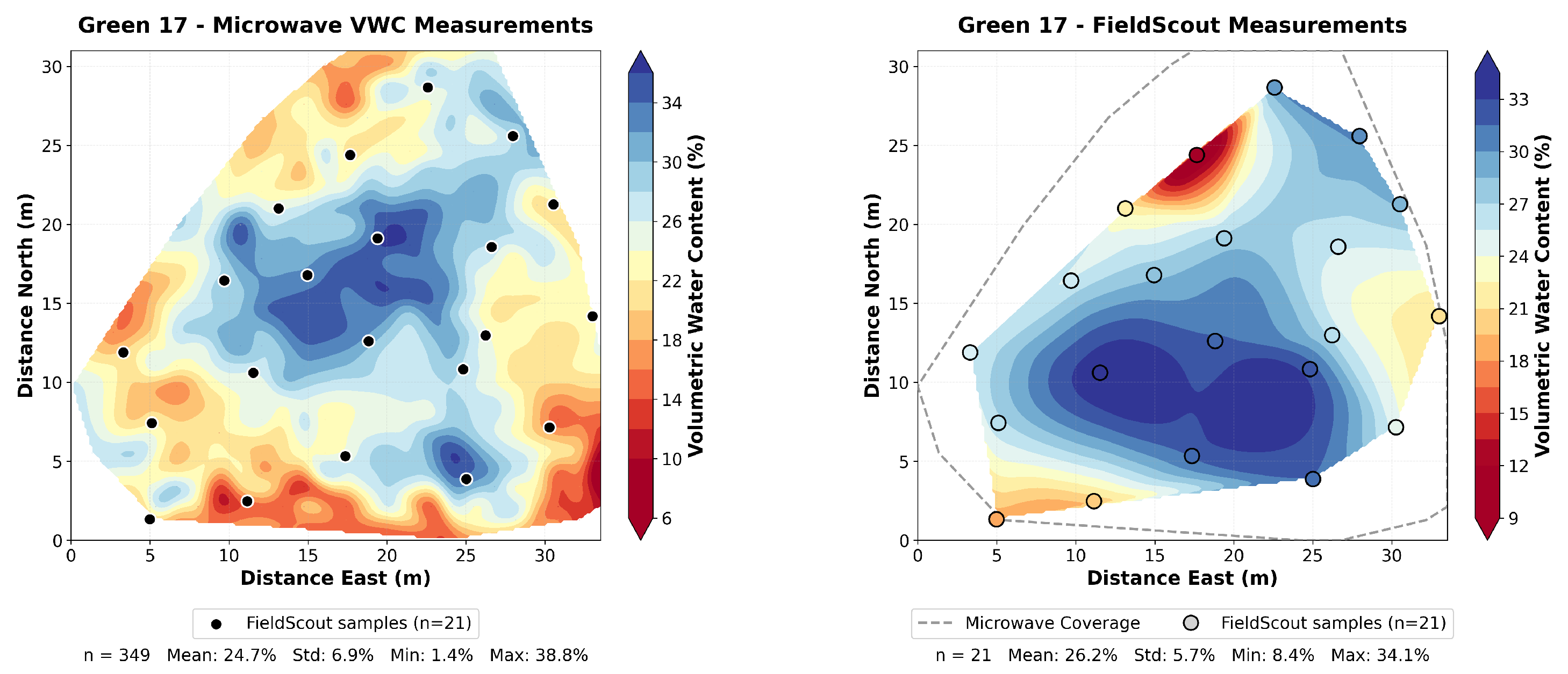
Figure 11, Figure 12, Figure 13, Figure 14 and Figure 15 show the spatial distribution of VWC from the microwave radiometer alongside the interpolated FieldScout measurements for each green on 13 January 2026. For display only, the FieldScout point measurements were interpolated onto a regular grid using cubic interpolation. Average VWC varies between greens, from 24.8% on Green 17 to 31.5% on Green 16, probably reflecting differences in irrigation history, drainage, and rootzone characteristics at the time of measurement. Within-green variability is pronounced on all greens, with standard deviations ranging from 6.8% (Green 17) to 13.6% (Green 10). The patterns differ green by green. Green 10 has a dry perimeter around a wetter centre. Greens 11 and 13 carry a northwest-to-southeast moisture gradient, drying toward their southeastern edges. On Green 16 a wet zone sits in the east-central area, ringed by drier margins, and Green 17 has a localised wet spot in the centre-north with drier conditions along the southern edge.

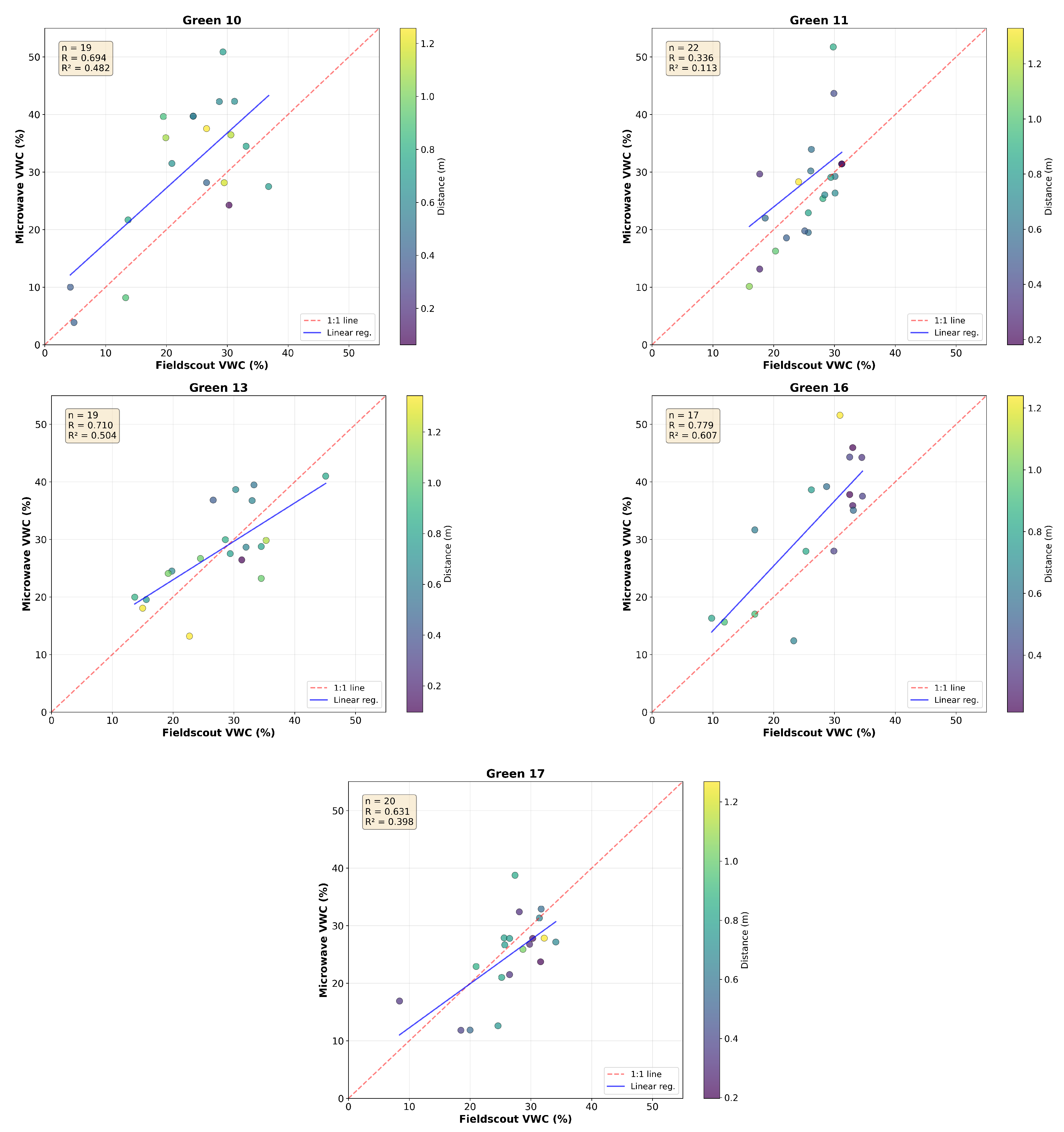
Figure 16 shows the FieldScout-microwave VWC correlation for all five greens. We matched each FieldScout sample location to the nearest microwave measurement within 1.5 m, retaining 97 of the 104 sampled points; the remaining seven had no microwave measurement within that radius. The matched probe points do not always sample the soil directly beneath the microwave sensor (Section 8).

Table 3. Microwave vs. FieldScout validation statistics per green. The per-green debiased RMSE is computed after removing the per-green mean bias, and measures the point-to-point random error, not the absolute-scale offset. Microwave values are the nearest measurement within 1.5 m of each probe point. All matched points are retained, including the two Green 11 outliers discussed in the text. Also, as mentioned in the text, validation points were chosen purposively, so the per-green R² is not directly comparable to studies using random or gridded sampling.

Green	R${⁠}^2$	Bias (%)	RMSE${⁠}_{\mathbf{debiased}}$ (%)
10	0.48	+7.1	8.8
11	0.11	+3.2	11.4
13	0.50	+0.5	6.0
16	0.61	+6.2	7.2
17	0.40	−1.6	5.6
Mean	0.42	+3.1	7.8

lists R², bias, and the per-green debiased RMSE. The debiased RMSE removes the mean bias for each green before the residuals are computed, so it measures the point-to-point random error and is not affected by the offset in the absolute scale. R² cannot reach one, because the reference probe carries its own measurement error. The maximum R² depends on how much real moisture variation a green presents: where the reference readings span a wide range the probe’s error is a small part of the total and R² can be high, while on a nearly uniform green that error is most of the variation present, so R² stays low however accurate the radiometer.

Green 11 has the lowest R${⁠}^2$ of the five (0.11), but the value reflects the validation conditions rather than a sensor fault. It was the most spatially uniform green on the survey day, with FieldScout readings varying little across it (standard deviation 4.9% VWC, against 5.9 to 9.1% on the other greens), so the reference’s own uncertainty is a large fraction of the limited spread and holds the maximum attainable R${⁠}^2$ down. Two microwave outliers compound this: one point reads 64% VWC where the FieldScout reads 20%, and a second reads 52% where the FieldScout reads 30%. Removing the single worst point raises R${⁠}^2$ from 0.11 to 0.43 and lowers the debiased RMSE from 11.4 to 7.2% VWC; removing both raises R${⁠}^2$ to 0.46 and lowers the debiased RMSE to 5.6% VWC, in line with the other greens. The microwave pattern on Green 11 is consistent from session to session (Figure 7), which argues against a systematic radiometer problem.

8. Discussion

The debiased RMSE in Table 3 carries contributions from both the microwave sensor and the FieldScout reference, hence it overstates the microwave error. We separate the two by subtracting the reference uncertainty in quadrature,

$${\sigma }_{\mathrm{mw}}=\sqrt{{\mathrm{RMSE}}_{\mathrm{debiased}}^2-{\sigma }_{\mathrm{ref}}^2},$$

(11)

and report the result for two values of ${\sigma }_{\mathrm{ref}}$ (

Table 4. Error decomposition per green. The microwave random error is estimated as ${\sigma }_{\mathrm{mw}}=\sqrt{{\mathrm{RMSE}}_{\mathrm{debiased}}^2-{\sigma }_{\mathrm{ref}}^2}$ from the debiased RMSE (Table 3), for two choices of reference uncertainty: ${\sigma }_{\mathrm{ref}}=3.0\%$ (FieldScout instrument accuracy only) and ${\sigma }_{\mathrm{ref}}=4.8\%$ (instrument accuracy combined with the 3.8% representativeness term).

		${\mathit{\sigma }}_{\mathbf{mw}}$ (%) for ${\mathit{\sigma }}_{\mathbf{ref}}=$
Green	n	3.0	4.8
10	19	8.3	7.4
11	22	11.0	10.3
13	19	5.2	3.5
16	17	6.6	5.3
17	20	4.8	2.9
Mean		7.1	5.9

). The FieldScout TDR 350 has a manufacturer accuracy of 3.0% VWC, and removing this instrument term alone gives a mean ${\sigma }_{\mathrm{mw}}$ of 7.1% VWC. A further representativeness term of 3.8% VWC, derived below from the two co-located probes, accounts for the fine-scale soil heterogeneity sampled differently by a point probe and an areal footprint. Combining both into ${\sigma }_{\mathrm{ref}}=\sqrt{{(3.0\%)}^2+{(3.8\%)}^2}=4.8\%$ VWC lowers the radiometer error to 5.9% VWC. Because the 3.8% term is an estimate, we treat 5.9% as a lower estimate and report the microwave random error as lying between roughly 6 and 8% VWC. The upper end of this range, near 8%, is the debiased RMSE itself, the value ${\sigma }_{\mathrm{mw}}$ would take if the FieldScout were error-free; because the reference always carries error, the microwave random error lies below it.

Per-green biases against the FieldScout are small, ranging from −1.6% to +7.1% VWC with a mean of +3.1% (Table 3), and three of the five greens fall within ±5%. The radiometer shows no consistent over- or under-reading against this reference. Against the HydraProbe the biases are much larger and negative, because the HydraProbe reads about 12 percentage points higher. That offset is most likely caused by the HydraProbe calibration, not the radiometer.

The two handheld probes, inserted 0.2 to 0.5 m apart at each point, give a measure of the reference uncertainty. Across all five greens (104 paired readings) the two probes are strongly correlated ($r=0.85$). Despite the constant offset, the two probes measure relative moisture changes equally well. After removing the offset, the residual RMS between the two probes is 5.4 percentage points. For two independent point samples this gives a per-point representativeness of $5.4/\sqrt{2}\approx 3.8\%$ VWC, the value used for ${\sigma }_{\mathrm{ref}}$ above.

The 3.8% term captures only the spread between two point probes. The radiometer averages over a 75 cm footprint, within which local variation in compaction, thatch thickness, and drainage produces moisture variability that shows up as disagreement between the two sensors even when both are working correctly. The depth mismatch compounds this. On irrigated greens the surface dries faster than the deeper layers, so the radiometer and the probe rods weigh the soil column differently. Such differences are inherent to any comparison between point and areal sensors and cannot be removed by better calibration. Together these mismatch effects inflate the observed debiased RMSE and depress R${⁠}^2$ relative to what either sensor would achieve against a truly co-located reference.

The most directly comparable validation is portable L-band radiometry on golf course fairways. Sapkota et al. [1] reported an off-the-shelf PoLRa accuracy of 9% VWC RMSE ($R^2=0.36$) against TDR, improving to 2% ($R^2=0.82$) after site-specific calibration, and concluded that site-specific calibration is needed for accurate absolute mapping. Under controlled co-location, Zhang et al. [30] found PoLRa unbiased RMSE mostly below 5% VWC against a capacitance probe. The mean debiased RMSE here, 7.8% VWC, is in line with the off-the-shelf figure but short of what site-specific calibration achieves. The mean R${⁠}^2$ of 0.42 is slightly higher than the 0.36 Sapkota et al. [1] obtained without that calibration. Two differences explain the gap. Sapkota et al. [1] georeferenced their sampling points with differential GNSS to better than 0.15 m and synchronised reference and radiometer by flagging, whereas the matching here tolerates up to 1.5 m. Their best results also came from per-survey site-specific calibration, which this system deliberately avoids.

The probe validation covers five greens, but the polarimetric measurements cover every green, so we can map the interference across the whole course. The worst-affected green sits beside the clubhouse and maintenance shed, where motors and consumer electronics make L-band interference likely. The polarimetric correction reduced day-to-day map variability by 4 to 15 percent on the four greens with measurable interference, on two others by 1 to 2 percent, and elsewhere the fit returned zero and left the maps unchanged. The validation greens are quiet, apart from a marginal effect on greens 10 and 11, so the correction barely alters these maps and the spatial patterns they show. Conversely, the strongly interfered greens (1–4), where the polarimetric correction does the most work, have no probe comparison, so its effect on absolute accuracy there is untested.

The validation rests on a single field day at one course, with points chosen purposively rather than at random or on a grid. One climate and one rootzone construction were sampled: Melbourne’s temperate climate and USGA sand-based greens. What the field day establishes is plausibility on one course under the conditions sampled. Accuracy across seasons, climates, and turf types remains untested.

The per-green baseline $b_{\mathrm{std}}$ absorbs the constant component of the local RFI environment, the part that is stable over time and simply raises the brightness temperature floor at that green. If that environment changes, say through the installation or removal of nearby electrical equipment, the baseline lags the true offset until enough new sessions accumulate. Interference raises brightness temperature, so a baseline fixed while interference was strong sits too high. If the interference later weakens, the brightness temperature drops, and the system mistakes that drop for wetter soil. The algorithm cannot detect or correct this bias.

The physical temperature of soil and canopy is a second uncorrected term in $T_{\mathrm{B}}=\epsilon T_{\mathrm{phys}}$. The receiver temperature correction described above deals with drift in the electronics. It does nothing about variation in soil and canopy temperature over the eight-week deployment. We looked for that signature by comparing the calibrated $T_{\mathrm{B}}$ of all five greens with hourly air temperature from ERA5-Land data at the site. No significant correlation was found.

The radiometer operates without active temperature control, relying instead on the logged-temperature drift correction described above, which assumes the radiometric response varies linearly with instrument temperature. A temperature-controlled enclosure holding the LNA at a constant physical temperature would remove this assumption, eliminating a source of uncertainty and possibly improving inter-day calibration consistency.

Taking this system beyond turf would mean revisiting two design choices. Turf canopies attenuate the soil emission negligibly, and their millimetre-scale relief is far below the smooth-surface threshold (Section 2), so the scheme carries neither a vegetation nor a roughness correction. Agricultural crops and natural grasslands carry canopy water contents one to two orders of magnitude higher, and tilled or unmanaged surfaces have RMS heights comparable to the Rayleigh limit at L-band. Both terms would have to be reintroduced, and that is not simply a matter of adding parameters: a single nadir look provides no polarisation or angular contrast from which to separate them, so auxiliary data would be needed. The self-calibration is not specific to turf, but it does assume repeated visits and a moisture range held between consistent limits by management. Where the surface dries well past wilting, or rarely reaches the wet end, the accumulated distribution no longer aligns with fixed anchors and the anchoring step would have to be reformulated.

Other established methods measure within-field soil moisture by different means, each with its own coverage and sensing depth. A cosmic-ray neutron probe averages over a footprint far larger than a green in this study, returning one field-averaged value rather than a map [31]. Electromagnetic induction correlates strongly with soil water content but is normally surveyed at sparse discrete stations [32]. Capacitance probes read a small volume around a fixed access tube, so mapping spatial pattern this way means installing several [33]. All three sense deeper into the rootzone than the radiometer’s top few centimetres.

On the greens in this study, the VWC scale set by the calibration anchors spans 34 to 44 percentage points across the greens. The practical irrigation decision band, the range within which a superintendent chooses to irrigate or wait, is narrower still, roughly 5–8 percentage points around the refill point. A random error of around 7% VWC therefore limits individual absolute readings for irrigation scheduling. The relative spatial patterns are detected reliably regardless of the absolute offset. Therefore, the mower-mounted system is useful for its spatial coverage, not for per-point absolute accuracy because that error is still small enough to separate wet zones from dry zones where the total VWC range spans 15–25 percentage points.

The persistent spatial patterns, and the slow changes in those patterns over time, are what support day-to-day decisions. A persistent dry zone may signal hydrophobic soil, compaction, or poor sprinkler coverage. On sand-based greens in warm climates hydrophobic soil is common and calls for wetting agents. Persistently wet zones on closely mown greens are disease-prone; locating them on daily maps allows targeted fungicide application and reduces chemical inputs.

Daily revisit makes trend monitoring possible in a way that periodic manual surveys cannot. A superintendent who applies a wetting agent or adjusts an irrigation zone reads off the following maps whether the pattern responded. On courses with variable-rate irrigation, the maps supply the spatial inputs needed to set sprinkler runtimes by zone. Without that hardware, they still direct hand-watering crews to the areas that need attention most. With suitable data infrastructure, the system produces moisture maps within minutes of mowing and can inform same-day irrigation decisions.

9. Conclusions

We have described an L-band digital polarimeter mounted on a golf course mower that produces dense spatial soil moisture maps during routine mowing. Previous studies have used dual-polarisation, vehicle-mounted L-band radiometers for turf with a Tau–Omega retrieval [9]. Here, full-Stokes polarimetry uses the unpolarised character of nadir soil emission for RFI mitigation, to our knowledge the first vehicle-mounted soil moisture radiometer to do so.

The spatial moisture patterns on all five greens are consistent from session to session, so the instrument resolves the real moisture structure of each green, and this repeatable mapping is its most useful output. The automated calibration converts brightness temperature to VWC by mapping each green’s accumulated $T_{\mathrm{B}}$ distribution onto calibration anchors at its dry and wet ends, without point-by-point field calibration. The absolute VWC scale depends on the assumed anchors. Per-green biases against the FieldScout reference are small, and once the reference probe’s own error is accounted for, the random error of the sensor is between roughly 6 and 8% VWC, estimated from a single field day. The relative pattern agrees between the radiometer and both handheld probes despite the absolute biases. The mean R${⁠}^2$ against the FieldScout is 0.42, enough to separate wet and dry zones for targeted management.

The main open question is whether the remaining biases shrink as sessions accumulate, or whether they reflect a systematic offset in the assumed anchors that the self-calibration cannot remove. The dry anchor is identical on every green and is never refined, so an error in it would bias every green in the same direction. The per-green bias instead runs in both directions, from −1.6% to +7.1% VWC. That argues against a shared systematic offset and points to green-specific effects. In Melbourne’s climate, thatch accumulation, topdressing programs, and seasonal root growth change the water held in the sensed surface layer through the year, so the wet end of the moisture distribution drifts and the high anchor is refined to follow it. Resolving the question, and testing how widely the method applies, calls for several follow-up studies. Multi-season monitoring would show how the absolute calibration behaves over longer time scales. Deployment on further sites and turf types would test its generality. A study relating the calibration anchors to independently measured field capacity and wilting point, including their sensitivity to initial values, would tie the scale to physical quantities. Centimetre-accurate co-location of reference probes with the sensor footprint would separate radiometer error from reference disagreement.