Ionospheric Response to Geomagnetic Storms of Different Intensity in the Eastern North Atlantic Mid-Latitudinal Zone (Iberian Peninsula, Azores and Madeira)—Part 1: Solar and Geomagnetic Drivers

Highlights

What are the main findings?

• The ionospheric response to geomagnetic storms was assessed using 80 events during the declining phase of the 24th solar cycle, focusing on the West-European middle latitudes.
• Statistical patterns were established relating the geomagnetic storm strength, solar wind source, and commencement type on the one hand, and the type, duration, and peak ionospheric response on the other hand.

What are the implications of the main findings?

• The identified patterns may be used to develop dedicated models of the ionospheric response to geomagnetic storms.

Abstract

The ionospheric response to a geomagnetic storm depends on several factors, including the strength of a storm, commencement type, solar origin of a geomagnetic storm (as, coronal mass ejections or high-speed solar wind streams), and observational site location. In this work, we present the results of a statistical analysis of 80 moderate to major geomagnetic storms that took place during the declining phase of the 24th solar cycle from 2015 to 2019. We performed an analysis of the ionospheric response to these storms using the total electron content (TEC) data obtained from three geodetic receivers located in Portugal: Lisbon (Continental Portugal), Furnas (Azores), and Funchal (Madeira). Statistical analysis of the observed TEC variations allowed detection of specific patterns in the ionospheric response to storms with different characteristics. We found that the type of geomagnetic storm commencement (gradual or sudden) is a statistically significant predictor of the ionospheric response amplitude and duration. Also, specific patterns in the ionospheric response to geomagnetic storms were found for the most southern location (Madeira), which are likely related to its proximity to the northern boundary of the equatorial ionization anomaly.

1. Introduction

Empirical models are one of the most actively developed types of ionospheric models. They are based on observational data and statistical analysis of such data, aiming to relate observed variations of parameters such as total electron content (TEC) to external forcings like solar flares, geomagnetic storms, and other space weather events [1,2]. These models are developed on different spatial scales, ranging from global to regional or even single-location models. Recent advances in neural network (NN) development have resulted in an explosive growth of new ionospheric models, which typically provide better forecasting quality than classical empirical models that rely on statistical, regression, or correlation analyses; see [1,2] and references therein.

The forecasting quality of empirical models is not uniform. They provide low-error forecasts for quiet periods—periods without solar flares or geomagnetic storms, but (geomagnetic) storm-time forecasting is still a significant challenge [1,2,3].

Geomagnetic storms (GM storms) are an important space weather phenomenon that, apart from affecting ground- and satellite-based technological and high-frequency communications systems, can severely affect the dynamics and structure of the Earth’s entire thermosphere and ionosphere. The ionospheric response to a geomagnetic storm is called an ionospheric storm or disturbance (here, we use the term “ionospheric disturbance” to distinguish it from a “geomagnetic storm”) and describes the variations in ionospheric conditions only due to geomagnetic events. Ionospheric variations can be determined from the TEC, the critical frequency of an ionospheric layer (e.g., f₀F2 for the F2 layer), or the peak electron density of an ionospheric layer (e.g., N_mF2 for the F2 layer). These parameters show specific variations, either an increase or decrease relative to their average quiet-time levels, which are defined as positive or negative ionospheric storms, respectively [4,5]. The type (positive or negative) of the ionospheric response to a GM storm depends on many conditions. These conditions include the strength of a geomagnetic storm, the local time of its commencement, the season, the solar activity level (which affects the dominant type of solar source triggering the GM storm), and the latitude and longitude of a location of interest.

Unfortunately, there has been little long-term research on ionospheric disturbances caused by GM storms. Most of the available studies concentrate on a limited set of notable geomagnetic events. Case studies help in understanding ionospheric behavior under certain conditions, but they tend to focus on strong storms or particular space weather events. As a result, they are not suitable for identifying statistical trends in the ionospheric response to GM storms, particularly for weak and moderate events.

Furthermore, as is shown by both long-term studies and individual case analyses, the ionospheric response to a storm is not spatially uniform and varies across latitudes and longitudes. Longitudinal dependency is not only due to different local times across zones but also due to regional peculiarities, such as the geomagnetic equator position or regional atmospheric features [6]. Among the long-term studies of ionospheric storm-time behavior, we would like to highlight specific studies [7,8,9,10]. The first two studies present analyses of events observed in the Euro-African longitudinal sector, while the last two focus on the American sector. In general, there is a strong similarity in the results obtained for middle and low latitudes (which are the focus area for our study) across different longitudinal sectors; however, some differences can be found even within the same longitudinal zone [9].

To summarize the results of [7,8,9,10], the ionospheric response to a GM storm at middle-to-low latitudes is most often positive, especially for GM storms that start during the daytime. For storms commencing at night, negative ionospheric disturbances or delayed positive disturbances occurring the next day are more frequent. Another important parameter affecting the response is the type of GM storm commencement (SC): gradual or sudden (GSC or SSC, respectively). GSC geomagnetic storms more frequently produce a delayed ionospheric response. In contrast, SSC storms, which trigger a negative disturbance, show higher peaks in ionospheric parameter variations than other events [7,8]. Also, refs. [7,8,10] show that more negative disturbances occur at lower latitudes than in mid-latitudinal regions. Some features of the storm-time response are the same across all longitudinal sectors, while others change significantly [10,11].

Thus, developing a good empirical regional ionospheric model requires a thorough preliminary study of the regional ionospheric response to different kinds of geomagnetic storms (onset time and type, season, solar origin, etc.). While NNs and other machine-learning techniques can identify specific patterns on their own, outperforming regression models [2,3], their forecasting quality during GM storm periods remains insufficient. Incorporating pre-identified relationships between certain GM storm characteristics and the ionospheric response at a given region or location seems like a logical step in developing the next generation of empirical models for ionospheric storm-time variations.

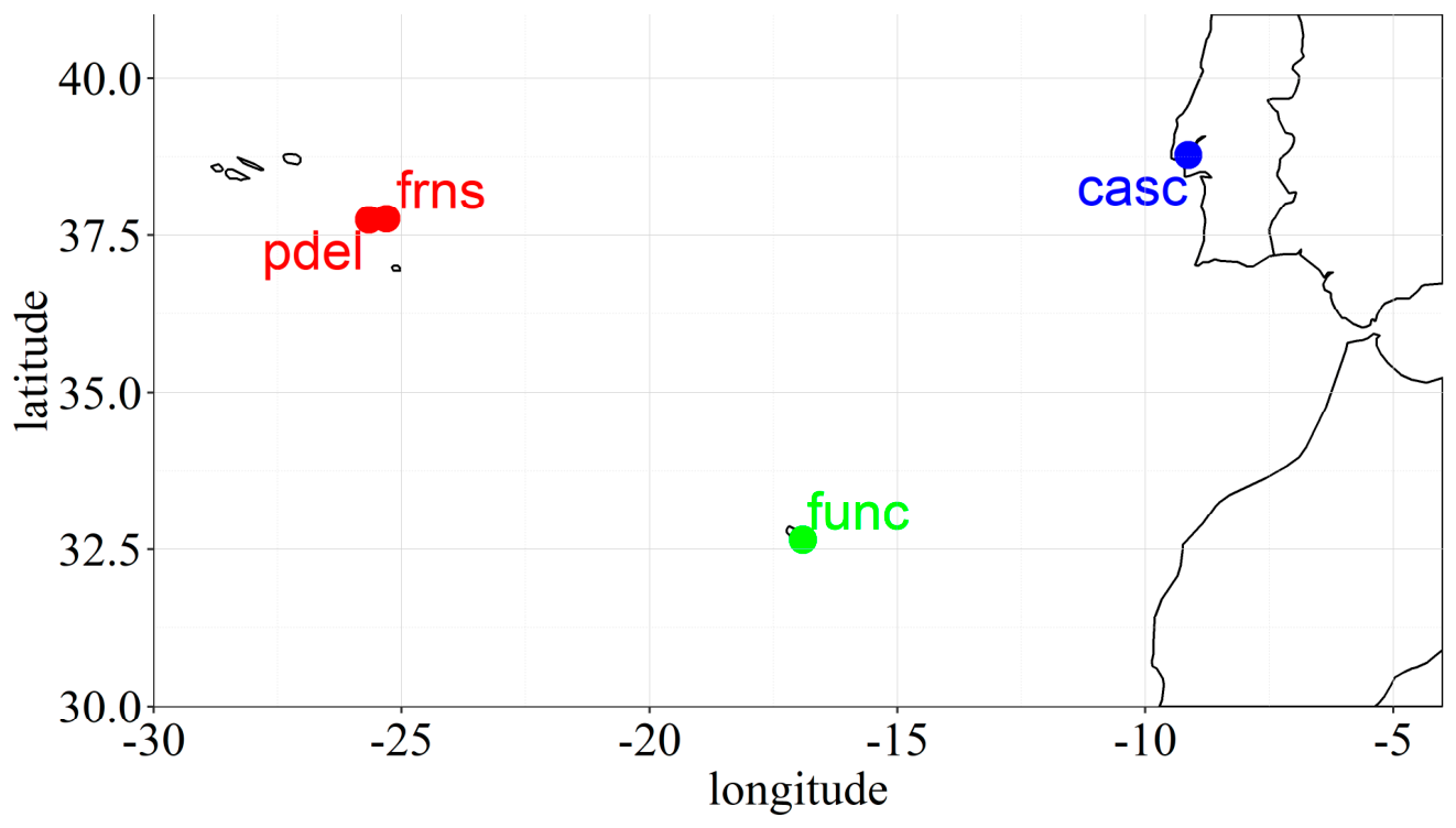
This study aims to identify these relationships and the most prominent patterns in the regional ionosphere’s response to GM storms. The study is focused on the statistical analysis of the storm-time ionospheric response in the middle-to-low latitudes (30°–40°N) of the eastern North Atlantic region (25°–0°E). A previous case study of ionospheric disturbances associated with several intense-to-major GM storms over the last decade showed notable differences in ionospheric responses between locations at 40°N and 30°N (Lisbon and the Azores islands, and Madeira, respectively) [12]. This difference was confirmed by modeling the ionosphere at those locations [2]: the models were trained on local ionospheric data (TEC) and a set of space weather parameters, including geomagnetic indices and solar wind parameters. The forecasting quality of the models developed for Madeira was slightly lower than for more northern locations (Lisbon and the Azores), suggesting other forcings not accounted for by the models (presumably, coupling with the low-latitudinal and equatorial ionosphere). To further examine similarities and differences in the ionosphere’s longitudinal and latitudinal response to GM storms, we performed a long-term statistical analysis of a wide range of GM storms observed during the last 5 years of the 24th solar cycle (2015–2019). In this paper, we present the results of the statistical analysis of such characteristics of ionospheric variations at Lisbon, the Azores, and Madeira, including their type, duration, and peak response in relation to solar conditions (solar activity level, solar sources of GM storms) and geomagnetic conditions (strength of GM storms, their commencement type).

2. Data

2.1. Total Electron Content Data

The ionospheric TEC data used in this work cover the time interval between January 2015 and December 2019, corresponding to the decreasing phase of the 24th solar cycle. The TEC data were collected at three Portuguese locations (see

Table 1. Coordinates of the GNSS receivers.

Code	Name	Latitude	Longitude
CASC	Lisbon/Cascais, Continent	38.7°N	9.14°W
FRNS 1	Furnas, Azores/S. Miguel	37.8°N	25.4°W
PDEL 2	Ponta Delgada, Azores/S. Miguel	37.8°N	25.8°W
FUNC	Funchal, Madeira	32.7°N	16.9°W

¹ Data are available for January–June 2015, 2017–2019. ² Data are available for July 2015–December 2016.

and Figure 1): Lisbon (Cascais) in Continental Portugal, either Furnas or Ponta Delgada on S. Miguel Island of the Azores archipelago (see Table 1 for details), and Funchal in Madeira.

The TEC data are derived from the GNSS (Global Navigation Satellite System) RINEX (Receiver Independent Exchange Format) files. Two data sources were used:

• The data from January to June 2015 and from January 2017 to December 2019 are from GNSS receivers of the national network of geodetic receivers RENEP (Rede Nacional de Estações Permanentes GNSS, https://renep.dgterritorio.gov.pt/ (accessed on 30 June 2026).
• The data gap (from July 2015 to December 2016) in the RENEP data was filled with the data available at the EUREF Permanent GNSS Network (EPN, https://www.epncb.oma.be/_networkdata/data_access/, accessed on 30 June 2026). The receivers of the RENEP and EUREF databases used in this study are the same receivers. The EUREF database was used because the data are not available at RENEP due to internal issues.

RENEP provides data in the RINEX 2.11 format. These files were processed and calibrated using the GNSS Lab (http://www.gnss-lab.org/ (accessed on 30 June 2026) and TEQC (25 February 2019 final release, https://www.unavco.org/software/data-processing/teqc/teqc.html (accessed on 30 June 2026; see the website for updated information about the manufacturer and currently available versions) software as described in [12]. EUREF provides data in the Compact RINEX format. These files were processed and calibrated using the GPS-TEC (v. 3.5) software by G. Seemala (https://seemala.blogspot.com/, accessed on 30 June 2026) [13]. Preliminary tests indicated that using different software to process RINEX files does not introduce any significant bias to the calculated TEC data.

The TEC data are in TEC units (1 TECu = 10¹⁶ electrons/m²). All the TEC series used in this work have 1 h time resolution.

2.2. Geomagnetic and Solar Data

The geomagnetic storms were identified and characterized using the Dst and Kp geomagnetic indices obtained from the Kyoto World Data Center (WDC) and from GFZ Helmholtz Center, Potsdam, Germany, respectively. Only moderate to major geomagnetic storms were studied. During the studied period, from January 2015 to December 2019, we identified 81 geomagnetic disturbances with Dst_min ≤ −50 nT. The storms were classified by the minimum Dst and maximum Kp values observed during the storm: moderate GM storms with −100 nT < Dst_min ≤ −50 nT (Kp_max not higher than 5), intense storms with −200 nT < Dst_min ≤ −100 nT (Kp_max between 6 and 7), and major storms with Dst_min ≤ −200 nT (Kp_max = 8).

The main sources of geomagnetic storms are coronal mass ejections (CMEs) and corotating interaction regions that produce corotating streams, or high-speed solar streams (HSS). CMEs are the primary cause of the largest and most severe space weather events, and their occurrence rate peaks during the maximum phase of the solar activity cycle. HSS are predominantly generated in coronal holes and interact with the slow solar wind, becoming more frequent during the declining phase of a solar cycle [14]. When a strong shock wave—typically driven ahead of a CME—rapidly compresses the magnetosphere, it produces a sudden storm commencement (SSC). Conversely, magnetic storms associated with HSS generally exhibit a gradual decrease in the geomagnetic field, referred to as storms with a gradual commencement (GSC).

All GM storms addressed in this study were categorized by their strength (using the Dst and Kp indices, see above), commencement type (SSC or GSC), solar activity level, and associated solar wind structures (“solar origin”). The solar origins were determined following the classification framework proposed by [15,16,17]: coronal mass ejections (CME), corotating streams or HSS, and slow solar wind (SW).

The solar wind parameters and the sunspot number data were obtained from the OMNI database.

2.3. Solar and Geomagnetic Activity During the Studied Period

The studied time interval (2015–2019) falls on the declining phase of the solar 24th cycle (see Figure 2 and the annual mean sunspot numbers in

Table 2. Annual means of the solar (sunspot numbers, SSN) and solar wind sources of GM storms.

Year	SSN	Number of Events at		Number of Storms Caused by
		Lisbon/Azores	Madeira	CME	HSS	SW
2015	70	31	30	12	10	9
2016	40	19	19	3	6	10
2017	22	17	17	5	8	4
2018	7	7	6	1	4	2
2019	4	7	7	1	4	2
Total number of events		81	79	22	32	27

). GM storms happening at different phases of solar activity are known [14] to have different dominant solar sources: CME-driven GM storms are observed more frequently near the solar maximum, while the peak of the HSS-driven GM storms takes place at the declining phase. As one can see from Table 2 and Figure 2, the number of all types of GM storms decreases from 2015 to 2019; the most drastic decreases is observed for the CME-caused storms (from 12 to 1 per year); the HSS-caused storms decrease from 10 to 4 per year; the number of GM storms associated with SWs decreases from 9 to 2 per year. An interesting feature of the declining phase of the 24th solar cycle is the sudden increase in solar activity, and consequently, in the number of GM storms, in 2017 compared to 2016 and 2018. Furthermore, as shown in Table 2, the number of GM storms caused by CME, HSS, and SW was roughly equal in 2015 (ranging from 9 to 12). In 2016, the majority of GM storms were driven by slow wind structures, whereas starting in 2017, HSS became the dominant source of GM storms.

Naturally, the number of ionospheric disturbances caused by GM storms decreases from 2015 to 2019 following the GM storms’ dynamics (Table 2).

3. Methods

3.1. TEC Variations

Variations of TEC (ΔTEC) during geomagnetic storms were studied as a difference between the observed TEC and the quiet TEC daily variation, TEC_QD (Equation (1)):

ΔTEC (h) = TEC (h) − TEC_QD (h)

(1)

To calculate TEC_QD, five geomagnetically quietest days of a month (days without geomagnetic disturbances) were selected. For each hour (h), from 0 to 23 h, the quiet TEC values (TEC_QD) are calculated as an average of TEC values for this hour for 5 quiet days of a month (Equation (2)). In case an analyzed event took place at the very end of a month, the TEC_QD values from the following month were used to account for the seasonal TEC variations.

$${\mathrm{TEC}}_{\mathrm{QD}}\left(\mathrm{h}\right)={\displaystyle \frac{1}{5}}\sum _{\mathrm{i}=1}^5{\mathrm{TEC}}_{\mathrm{i}}\left(\mathrm{h}\right)$$

(2)

Only ΔTEC values exceeding the limit of ±2σ were considered to be statistically significant, where σ is the standard deviation calculated using all available TEC data for a studied month without hourly binning (single value for each month and for each location). While in general the usage of a single σ value for all hours may result in a systematic omission of the night-time (between 22 h and 8 h) minor ionospheric disturbances, for the studied data set we observed only five such events, and only in two cases these disturbances were classified as non-statistically significant at one or two of the locations. Thus, the usage of a single σ threshold does not affect the results of our analysis.

When data were available, each storm event was analyzed over a six-day window, spanning from two days prior to storm commencement to three days after. The TEC data for the three locations (Continent, the Azores and Madeira) were studied separately to assess the similarity/differences in the locations separated in longitude (for example, Continent vs. the Azores) or latitude (for example, Continent vs. Madeira).

For each of the studied GM storms, the first ionospheric peak response (ΔTEC_p) and its absolute value (|ΔTEC_p|), the type of the response (positive for ΔTEC_p ≥ +2σ, negative for ΔTEC_p ≤ −2σ, or zero for |ΔTEC_p| < 2σ), and the duration of the statistically significant ionospheric response (in days) were calculated.

The ionospheric disturbances were classified by the type of ΔTEC variations during up to 3 days after the GM storm commencement. The 1st day of the ionospheric disturbance was defined as the 1st day after a storm commencement when the ionosphere can respond to a geomagnetic storm. Depending on the SC time, it is either the 1st day of a geomagnetic storm if a GM storm started before sunrise or the next day after SC if a storm began after sunset (see examples in Supplementary Material S1, Figures S2 and S4, respectively).

Depending on the values of ΔTEC, the ionospheric response was classified as positive (p), negative (n), or zero (0). The classification was applied up to the 3rd day of the ionospheric disturbance. Ionospheric variations observed after the 3rd day were not considered in this study because of the ambiguity of the interpretation of the sources of those disturbances. Thus, we defined the ionospheric response in three groups, 0.*, p.* and n.* types, with * showing possible sub-types: for example, the group p.* includes the 1-day-long p disturbance, the 2-day-long p.p and p.n disturbances, and the 3-day-long disturbances, such as p.p.p and so on. Examples of the different types of ionospheric disturbances are shown in Supplementary Material S1, Figures S1–S9. Please note that the 0-type ionospheric disturbance is equivalent to the 0-day-long disturbance: both classifications mean that there was no statistically significant ionospheric response to a GM storm. Our definition of the 0-type disturbance is not affected by the data gaps: in case the type or the peak response cannot be identified due to a data gap, this event was excluded from the respective set of analyzed events.

3.2. Statistical Analysis

In this study, we evaluated the mean percentages of ionospheric disturbances categorized by disturbance type and duration, alongside the relative proportions of specific ionospheric responses as a function of solar and geomagnetic parameters. To assess the statistical significance of the observed variations, we applied Fisher’s exact test to compute the probability (p-value) of the null hypothesis—stating that no true difference exists between compared subsets. Fisher’s exact test was selected because several subsets contained small sample sizes, rendering the standard χ² test inapplicable.

To compare the peak response (ΔTEC_p) values obtained for different subsets, we used the standard error (SE) thresholds.

4. Results

Our objective here is to identify patterns in the ionospheric response of geomagnetic storms using statistical analysis. As the parameters of the ionospheric response to each of the studied GM storms, we used ΔTEC_p and |ΔTEC_p| values, both in TECu and in the units of σ, the ionospheric disturbance classification (p for positive and n for negative, and so on as explained above), and the duration of the ionospheric disturbance (in days).

As was mentioned in Section 2.2, during the studied time interval there were 81 geomagnetic disturbances with Dst_min ≤ −50 nT. For the Continent (Lisbon) and the Azores locations, the data are available for all 81 GM storms, while for Madeira the data are available only for 78 events due to the data gaps (see Table 2). Furthermore, sometimes short data gaps appear during storm time. In some of those cases, we have not been able to identify both the type of ionospheric response and the ΔTEC_p value, while in other cases we have identified the type but not the peak response. This resulted in slightly different numbers of the analyzed events for the same location but between the studied ionospheric parameters. The total number of events used in each case is shown in the corresponding Tables.

All the results of the analysis are presented in

Table 3. Number of ionospheric disturbances of different types (see classification in Section 3). Numbers in parentheses show the percentage of a certain type of ionospheric disturbances out of all geomagnetic storms; bold marks data for general types and italic marks data for sub-types. See Section 3.1 for the description of the types.

Type of the Event	Lisbon	Azores	Madeira
0.*	13 (16.0%)	15 (18.5%)	12 (15.4%)
0	9 (11.1%)	12 (14.8%)	8 (10.3%)
0.p.*	4 (4.9%)	3 (3.7%)	4 (5.1%)
0.n	0 (0%)	0 (0%)	0 (0%)
p.*	62 (76.5%)	62 (76.5%)	57 (73.1%)
p	38 (47.0%)	42 (51.9%)	37 (47.4%)
p.p.*	10 (12.3%)	6 (7.4%)	10 (12.8%)
p.n.*	10 (12.3%)	12 (14.8%)	9 (11.5%)
n.*	6 (7.4%)	4 (4.9%)	10 (12.8%)
n	4 (4.9%)	2 (2.5%)	6 (7.7%)
n.p	1 (1.2%)	1 (1.2%)	3 (3.8%)
n.n	1 (1.2%)	1 (1.2%)	1 (1.3%)
All events	81 (100%)	81 (100%)	79 (100%)

,

Table 4. Number of ionospheric disturbances of different durations. Numbers in parentheses show the percentage of a certain type of ionospheric disturbance out of the observed ionospheric disturbances (0-type is excluded); numbers in bold show the most abundant groups.

Ionospheric Response Duration	Lisbon	Azores	Madeira
0 days	9 (11.1%)	12 (14.8%)	8 (10.3%)
1 day	42 (51.9%)	45 (55.6%)	43 (55.1%)
2 days	22 (27.2%)	17 (21)	21 (26.9%)
3 days	8 (9.9%)	7 (8.6%)	6 (7.7%)
All events	81 (100%)	81 (100%)	78 (100%)

and

Table 5. Mean and standard error (±SE) values of the first ionospheric peak response for all, all positive, and all negative ionospheric disturbances (0-type is excluded). See Section 3.1 for the description of the types.

Parameter	Lisbon	Azores	Madeira
All storms
ΔTECp, TECu	8.4 ± 0.9	8.9 ± 0.9	8.6 ± 1.1
ΔTECp, σ units	3.2 ± 0.3	3.5 ± 0.3	3.0 ± 0.4
All storms
|ΔTECp|, TECu	9.8 ± 0.7	10.2 ± 0.7	11.3 ± 0.8
|ΔTECp|, σ units	3.7 ± 0.2	3.9 ± 0.3	3.8 ± 0.3
p.* storms
ΔTECp, TECu	10.9 ± 0.8	11.6 ± 0.9	12.6 ± 1.0
ΔTECp, σ units	4.1 ± 0.3	4.5 ± 0.3	4.4 ± 0.3
n.* storms
ΔTECp, TECu	−8.6 ± 1.7	−9.5 ± 3.1	−10.7 ± 1.8
ΔTECp, σ units	−2.5 ± 0.2	−2.7 ± 0.2	−3.1 ± 0.2

, Figure 3, Figure 4, Figure 5 and Figure 6, and in the Supplementary Material S2 (Tables S1–S5), Supplementary Material S3 (Tables S6–S10) and Supplementary Material S4 (Tables S11–S15 and Figure S10).

4.1. General Statistics of the Studied Sample

The absolute majority (70–75%) of the studied GM storms resulted (at least during the 1st day) in a positive ionospheric disturbance. About 65% of such GM storms (or ab. 50% of all storms) produced a single-day positive ionospheric disturbance (p sub-type); see Table 3.

Depending on the studied location, 10–15% of GM storms produced no disturbances in the ionosphere that exceeded the ±2σ threshold (0 type or 0-day-long). Additionally, ab. 5% of all events resulted in a non-significant ionospheric response on the 1st day but a significant positive response on the 2nd day of the GM storm. These values are similar across all studied locations (Table 3). Negative ionospheric responses (at least during the 1st day) were observed at Lisbon/Continent and the Azores during ab. 5–7% of GM storms, whereas for Madeira, this proportion was larger (~13%). This likely reflects the more southern location of Madeira relative to the continental and Azorean stations, as well as the effects produced by the equatorial ionosphere. Previous studies have reported distinct features in Madeira’s ionospheric response based on data analysis [12] and modeling; the present analysis confirms these findings using a larger dataset.

The duration of the ionospheric response to GM storms (number of days for which statistically significant ionospheric disturbances were observed), on average, shows no spatial patterns (Table 4). For all three locations, the 1-day-long ionospheric disturbances were observed in ~60% of the studied cases, the 2-day-long ionospheric disturbances took place in 23–30% of GM storms, and ~10% of GM storms produced the 3-day-long ionospheric disturbances.

In case an ionospheric disturbance lasts for 2 days, the probability of it being a p-type disturbance (p.p or p.n) is ~82% for the northern locations (18 out of 22 and 14 out of 17 events at Lisbon and the Azores, respectively) and 71% for the southern location (15 out of 21 events at Madeira). Also, at the Continental and Azorean locations the p.n ionospheric disturbances were observed more frequently than p.p ones: ~46% vs. 36%, respectively, for the Continent, and 59% vs. 24%, respectively, for the Azores, while for Madeira the number of p.p and p.n storms was about the same (38% and 33%, respectively). The origin of the higher incidence of positive ionospheric disturbances observed at the Azores remains unresolved; specifically, whether this reflects a true physical mechanism or an artifact of the dataset employed in this study. Further investigation is required to elucidate this finding. Positive disturbances observed only on the second day (0.p type) were observed in 1–5% of the studied events. The type 0.n of ionospheric response was not observed at all.

The average peak response to GM storms for different locations and different types of ionospheric disturbances is shown in Table 5. As one can see, the mean ΔTEC_p and the mean |ΔTEC_p|, both in TEC and σ units, are about the same at all observed locations: ~8.5 TECu (3.3 σ) for ΔTEC_p and ~10.5 TECu (3.8 σ) The average peak responses of the positive and negative ionospheric disturbances (in absolute values) are about the same in TEC units (12 TECu and −11 TECu, on average, respectively) but in σ units the peak response of the positive ionospheric disturbances is slightly larger (in absolute values): ~4.3 σ vs. ~−2.8 σ, on average, respectively. It must be noted that the limited number of n.* type ionospheric storms precludes statistically significant conclusions, except for the Madeira location.

4.2. Ionospheric Response Type

The p.* type ionospheric disturbances prevail during all the analyzed years (60–100% of the observed events), and there is no trend in their occurrence related to the decline of the solar activity—see Supplementary Material S2 (Table S1). 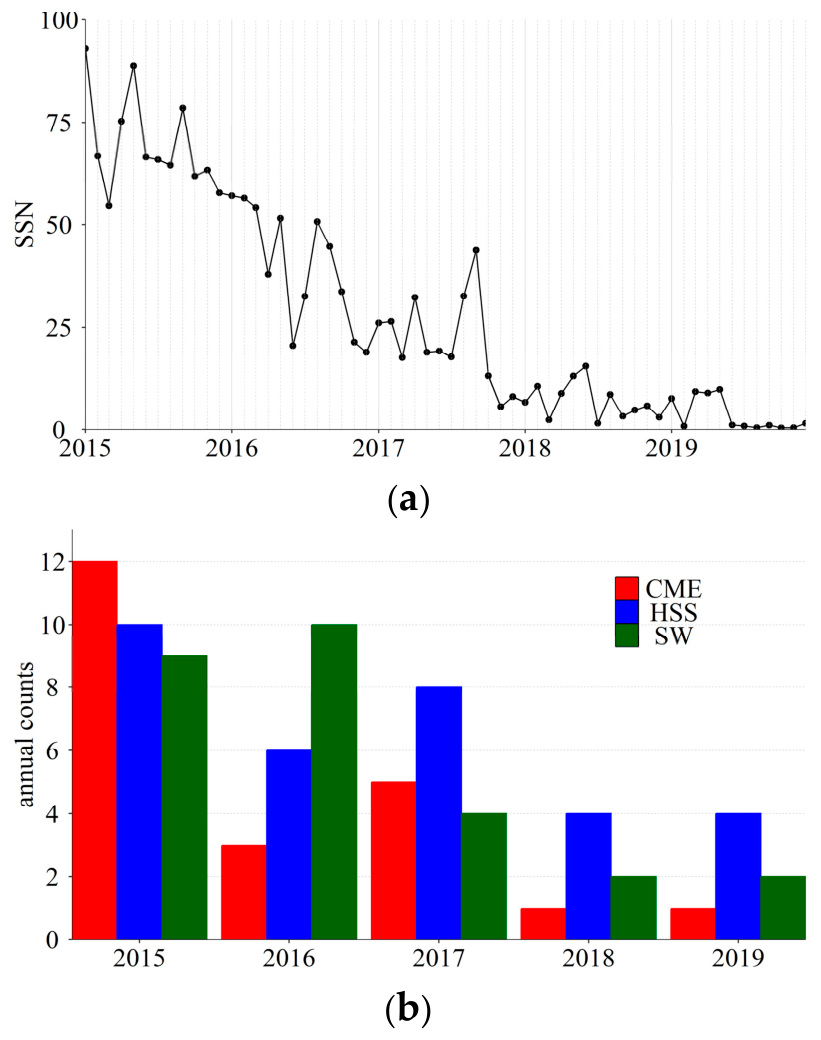The number of disturbances of the 0.* and n.* types is very small, from 0 to 7 events per year; thus, the conclusions on their time variations are not statistically significant (p-value = ~0.4); however, we must note that the negative ionospheric disturbances were observed only in 2015 and 2017 (plus one event in 2016, which was seen only at Madeira). This may be related to the solar activity behavior during those years: large numbers of CME- and HSS-driven GM storms in 2015 and 2017. The number of GM storms that resulted in no statistically significant ionospheric response (0-type) was 4 to 7 events per year in 2015–2016 and dropped to 0 events per year in 2018–2019. This trend may be related either to a simple decrease in GM storms following the decline of solar activity between 2015 and 2019, or to a change in the proportion of CME-, HSS-, and SW-driven storms. Unfortunately, because the number of storms for the 0-type and n-type is very small, conclusions regarding their temporal variations are not statistically robust.

To test the hypothesis on the relation between the ionospheric disturbance type and the solar source of GM storms, we studied the distribution of the 0.*, p.* and n.* types with the solar sources (CME/HSS/SW)—see also Supplementary Material S2 (Table S2). While the small number of the 0.* and n.* type ionospheric disturbances do not allow us to make statistically significant conclusions, it seems that the negative ionospheric disturbances are most often caused by the CME- and SW-driven geomagnetic storms. Also, for the locations at ~40°N, the 0.* type disturbances are more frequently associated with SW, while for Madeira there is no clear pattern. Thus, we assume that the relatively large numbers of the n.* type disturbances in 2015 and 2017 mentioned above can be associated with a larger number of the CME-driven GM storms. Concerning the positive ionospheric disturbances, 42–45% of the p.* type disturbances (at all locations) were caused by HSS geomagnetic storms, 30–32% were caused by GM storms associated with SW structures, and the rest, 26–27%, were related to CME-driven GM events. Unfortunately, because the number of events is small, the found dependence of the ionospheric response type on the solar sources is not statistically robust: the highest p-value = 0.23 was obtained for the Azores data.

To assess the dependence of the types of ionospheric disturbance on the strength of geomagnetic storms, we used the Dst and Kp indices. For the moderate geomagnetic events, the distribution between the types of the ionospheric response is not different from the distribution for the whole studied sample (see Table 3 and Supplementary Material S2: Tables S3 and S4), while for the intense geomagnetic storms we see, compared to the whole sample, fewer number of the p.* types of the ionospheric responses (66.5% vs. ~75% on average) and more n.* types (~16.8% vs. ~8.7% on average). Since there was only 1 major storm, no statistically significant conclusions can be made about such events on the frequency of different types of ionospheric response. Unfortunately, the small number of studied events leads to a low statistical significance for these results, and more data are needed to confirm these findings.

The results of the analysis show that the type of geomagnetic storm commencement, GSC or SSC, is a statistically reliable factor predicting the ionospheric response (see Supplementary Material S2, Table S5). Geomagnetic storms with GSC more frequently cause the 0.* type ionospheric response (24% compared to 16% for the whole sample) and less frequently cause ionospheric disturbances of the p-type (64% compared to 76% for the whole sample); also, at Madeira they cause n.* type ionospheric disturbances more frequently than the average (20% vs. 13%). Geomagnetic storms with SSC are more likely to cause the p.* type ionospheric disturbances (~86% vs. ~76%) and less frequently cause the 0.* type disturbances (~8% vs. 16%). The differences found are statistically significant with p-value = 0.16 for Lisbon, p-value = 0.02 for the Azores, and p-value = 0.05 for Madeira.

4.3. Ionospheric Response Duration

The duration of the ionospheric disturbance was also addressed in terms of its dependence on solar activity and the solar drivers of GM storms (see Supplementary Material S3, Tables S6 and S7). The number of short (1-day-long) ionospheric disturbances follows the temporal variations of the CME and HSS rates (Table 2). Comparing the data in Table 2, Tables S6 and S7, it can be concluded that the anomalous numbers of the CME- and HSS-driven storms in 2016–2017 were caused not by an increase in the number of such events in 2017 but by a decrease in the event numbers in 2016. The number of the 2-day-long events also follows the decrease in solar activity, but no specific pattern can be deduced from the data. Three-day-long ionospheric disturbances are rare (0–4 events per year), and no definite conclusions can be drawn on the temporal evolution of their appearance.

The HSS and the SW structures appear to be the most frequent drivers of the 1-day-long ionospheric disturbances, but about half of the CME-driven GM storms also produce 1-day storms. Concerning the 2-day-long ionospheric disturbances, it seems that the most frequent driver of such events is CME-driven geomagnetic storms, but HSS and SW structures can also cause 2-day-long events. Unfortunately, the small number of events per subset results in a low statistical significance of these results, which must be confirmed on larger datasets.

The dependence of the duration of the ionospheric response on geomagnetic storm strength is more prominent when Kp_max is considered instead of Dst_min (see Supplementary Material S3, Tables S8 and S9). The distribution of the ionospheric response duration for storms of different strengths (to be compared to the distribution for the whole sample shown in Table 4) for storms classified by the Dst index shows no significant patterns except for Madeira, where such GM storms seem to produce fewer 2-day-long disturbances compared to the average over the whole set (p-value = 0.11). On the other hand, if the Kp index is used for classification, several patterns can be identified. First, the geomagnetic events with Kp_max = 4 and 6 more frequently result in 2-day-long ionospheric disturbances than the average at the Azores and Lisbon (50% vs. 23% and 32% vs. 22%, respectively, p-value = 0.28 for Lisbon and p-value = 0.16 for the Azores). For geomagnetic events with Kp_max = 5, the pattern is the opposite: there are fewer 2-days and more 1-day ionospheric disturbances at the Azores and Madeira (12% vs. 23% and 65% vs. 54%, respectively, p-value = 0.16 for the Azores and p-value = 0.14 for Madeira). For geomagnetic events with Kp_max above 6, the number of events per subset is too small to make any conclusions.

The type of GM storm commencement is found to be a statistically significant factor predicting the duration of the ionospheric disturbances at the Azores (p-value = < 0.01). At this location, for the GSC events, the absence of the ionospheric response (0-day-long disturbance) was observed there about twice as often as the average (25% vs. 12%), while the 2-day-long storms were observed much less frequently than the average (7.5% vs. 23%). For other locations, no statistically significant differences between the duration of the ionospheric response to the GM storms with GSC and SSC were found.

4.4. Ionospheric Peak Response

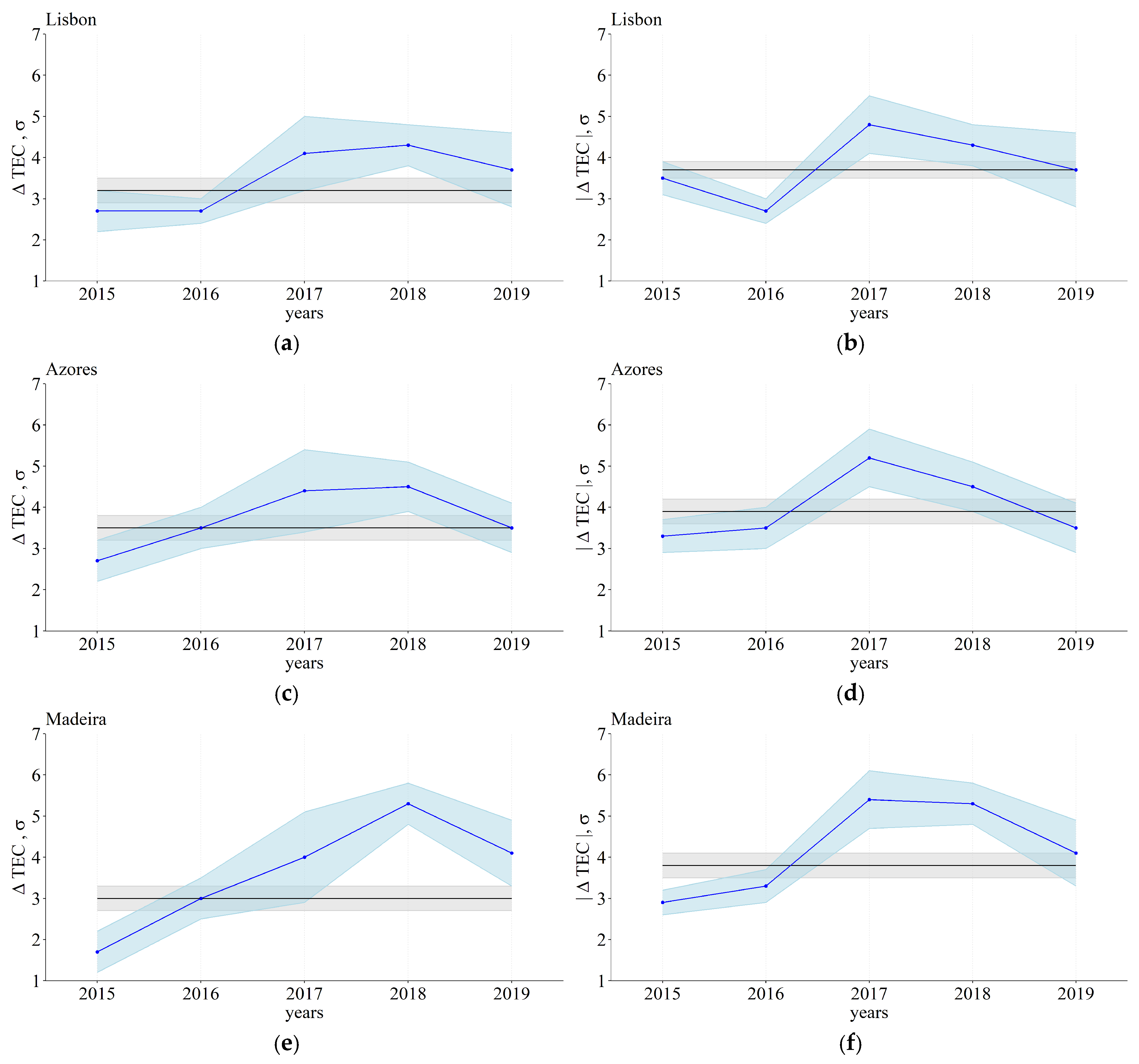
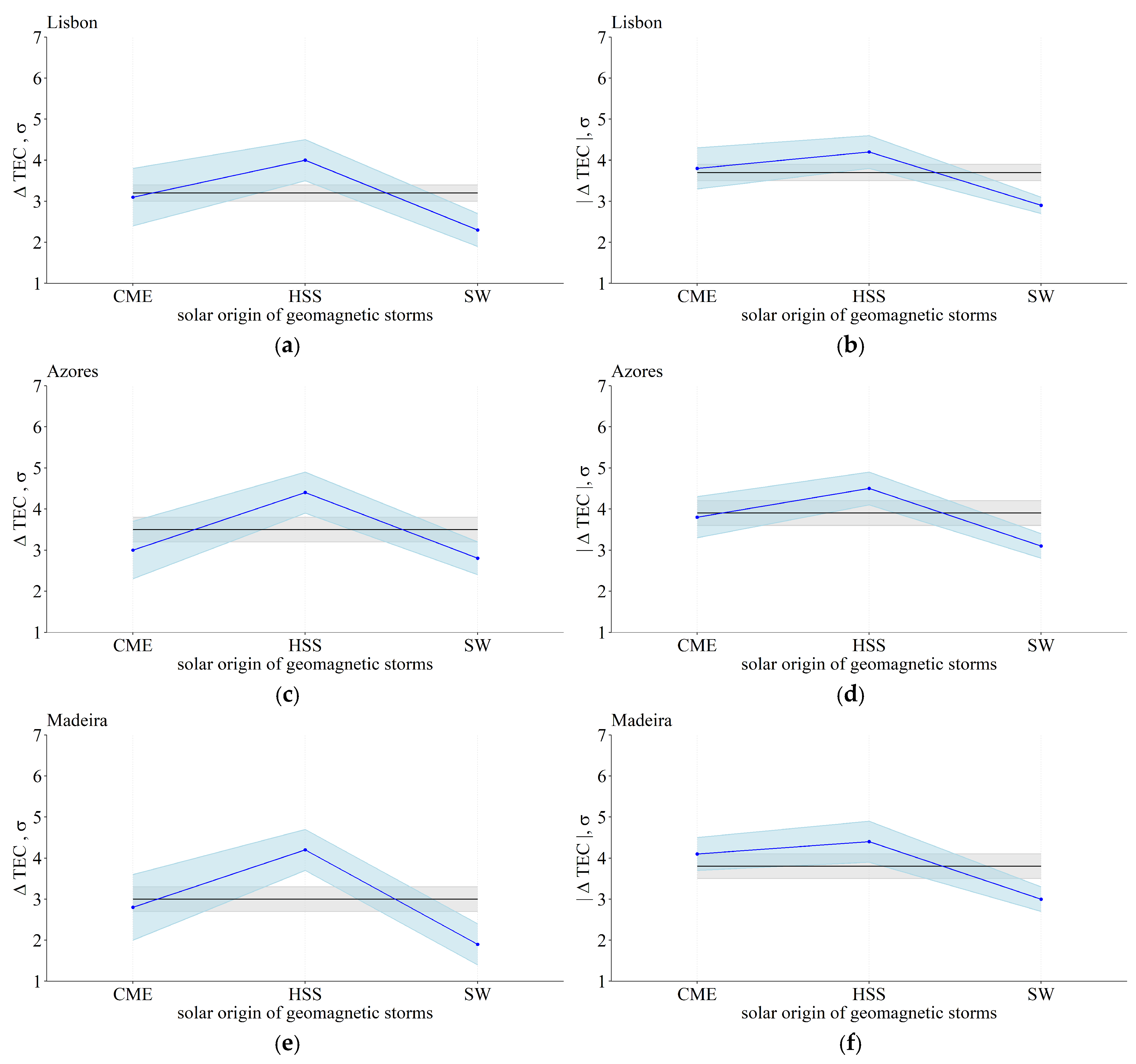
The variations in the amplitude of the first ionospheric response (peak response, ΔTEC_p and |ΔTEC_p|) to the GM storms of different years and associated with different solar sources were analyzed. The results are shown in Figure 3 and Figure 4 for ΔTEC_p and |ΔTEC_p| measured in σ units (for the results in TECu, please see Supplementary Material S4, Tables S11 and S12). The peak response measured in TECu decreases from 2015 to 2019 from 7–10 TECu to 5–6 TECu for ΔTEC_p and from 7–13 TECu to 5–6 TECu for |ΔTEC_p|. However, it seems that this decrease is related to the overall decrease of the TEC values between 2015 and 2019 caused by the decrease of the solar activity and the solar UV flux: the peak response measured in σ units (both ΔTEC_p and |ΔTEC_p|) remains more or less the same during this time interval (see Figure 3): 3–5 σ for ΔTEC_p and 3–7 σ for |ΔTEC_p|. Still, the ΔTEC_p values measured in σ units seem to be anomalously higher in 2018 at all stations (exceeding the 2 SE threshold), while for |ΔTEC_p| a statistically significant increase was observed in 2017. The difference between ΔTEC_p and |ΔTEC_p| is related to different rates of the p.* and n.* types of the ionospheric disturbances observed during these years (see Section 4.2 and Supplementary Material S2, Table S1).

In general, CME- and HSS-driven GM storms caused larger ΔTEC_p values compared to the SW-driven storms (Figure 4, also see Supplementary Material S4, Table S12): 9–13 TECu (3–5 σ) compared to 5–7 TECu (2–3 σ), respectively. The larger-than-average ΔTEC_p values for the HSS-driven GM storms (exceeding the 2 SE threshold) are related to a larger number of the p.* type ionospheric disturbances during such storms. The same is true for the |ΔTEC_p| values: CME- and HSS-driven GM storms are associated with a 10–14 TECu (4–5 σ) peak response, while SW-driven GM storms cause, on average, |ΔTEC_p| of 8–9 TECu (~3 σ)—this difference exceeds the 2 SE threshold.

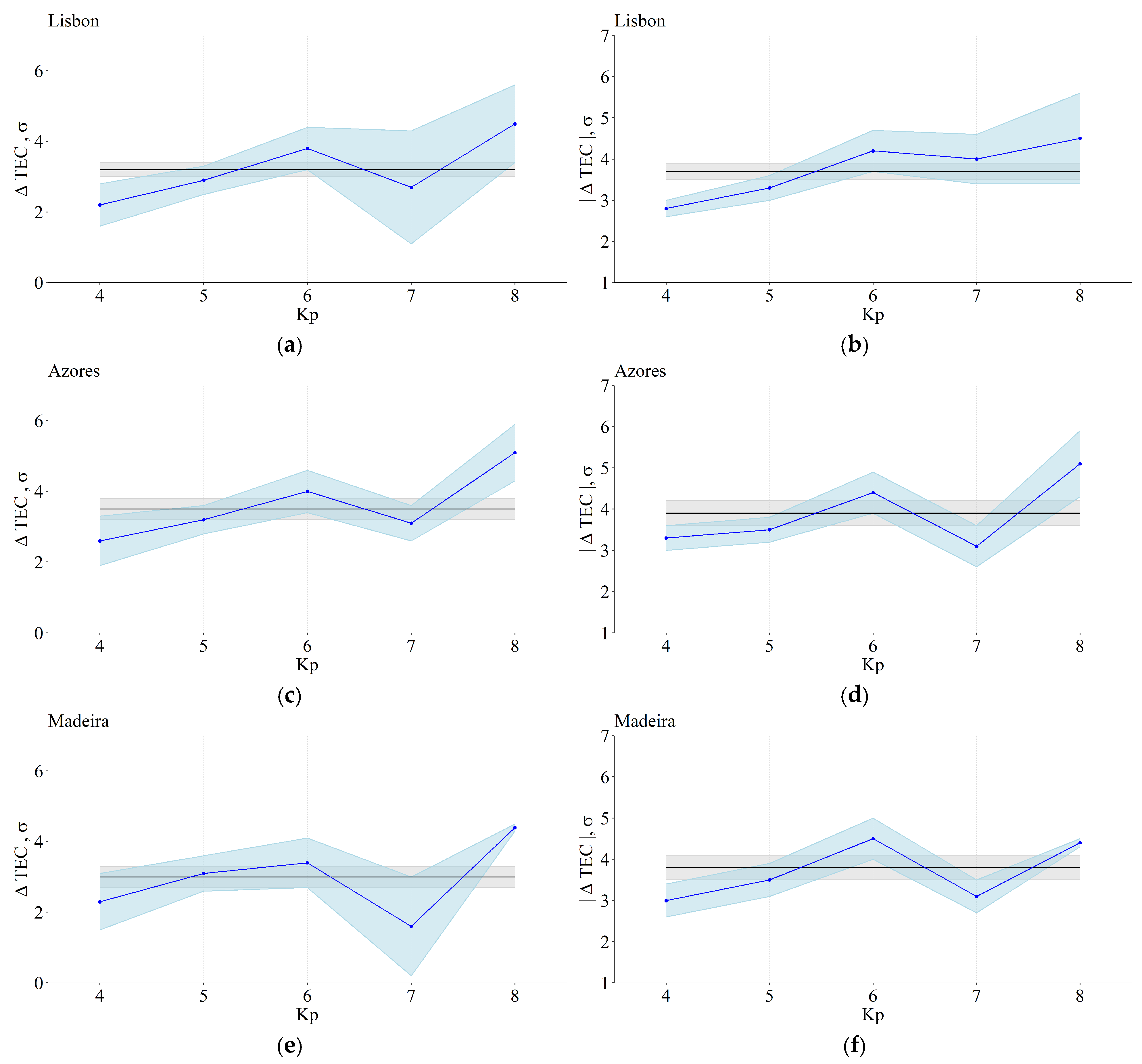
The changes in the peak response depending on the strength of the ionospheric storms are shown in Figure 5 and in Supplementary Material S4, Tables S13 and S14 and Figure S10. There is a general increase in the peak response following both the Dst_min and Kp_max values; however, statistically significant differences (at least at the 2 SE level) were found only for GM storms with Kp_max = 4 and Kp_max = 8.

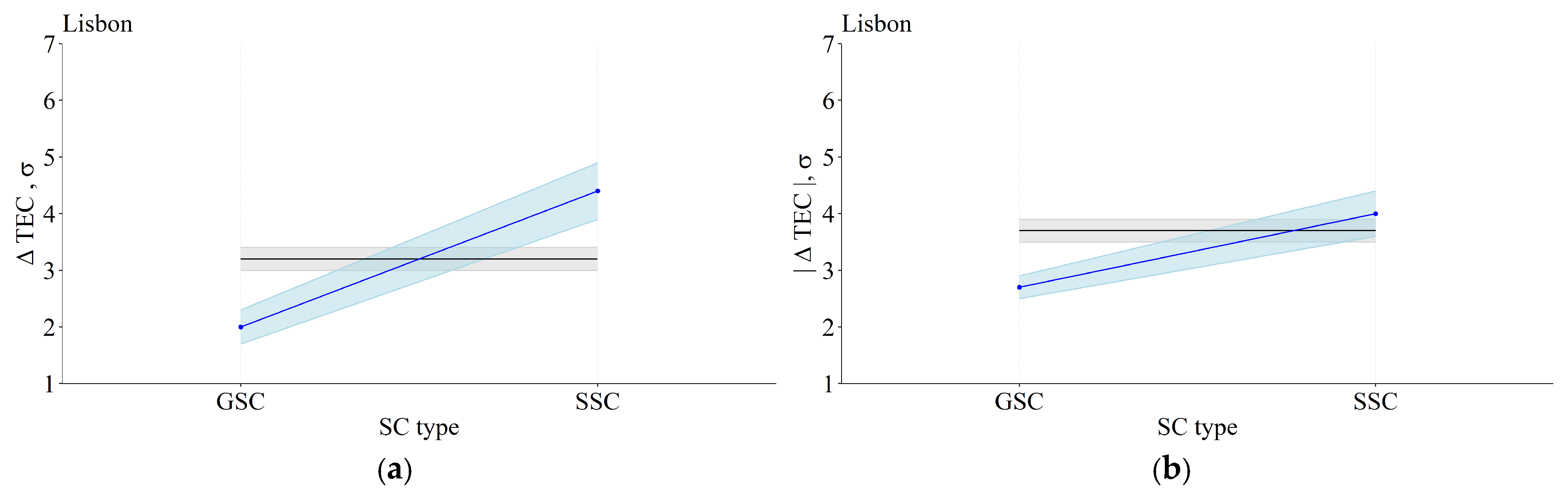
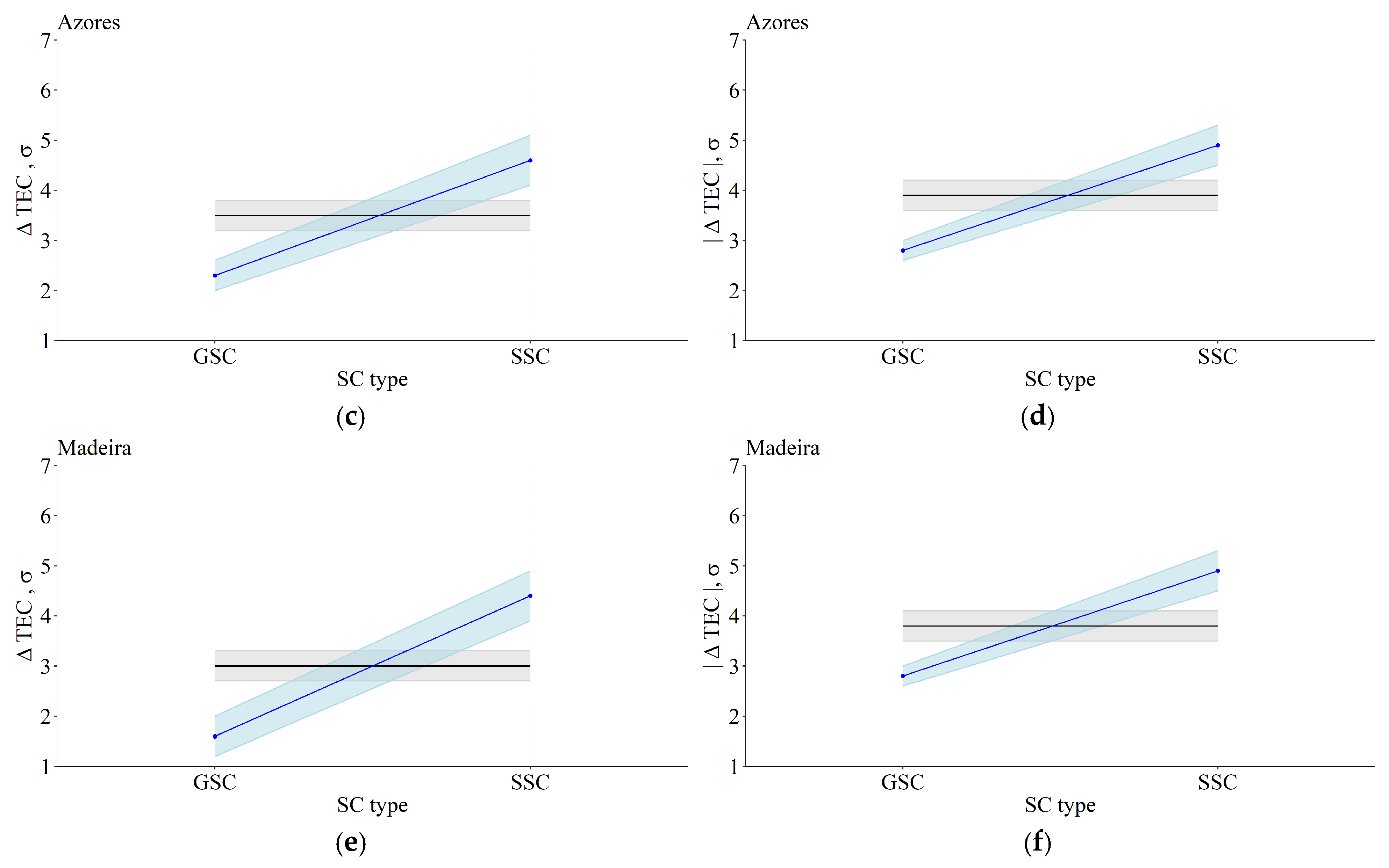
The type of GM storm commencement (GSC or SSC) is, similar to the ionospheric response type and length, a statistically reliable factor defining the amplitude of the ionospheric response. The values of ΔTEC_p and |ΔTEC_p| for GSC events are significantly (exceeding the threshold of ±2 SE) smaller than the average, especially if measured in σ units: ~2.3 σ vs. ~3.2 σ for ΔTEC_p and ~2.8 σ vs. ~3.9 σ for |ΔTEC_p|, while for the SSC events the peak response is 1.3–1.5 times larger than the average, both for ΔTEC_p and |ΔTEC_p|, both in TECu and in σ units—see Figure 6 and Supplementary Material S4, Table S15.

5. Discussion and Conclusions

Our results indicate that, in the studied locations, 85–90% of moderate to major GM storms result in ionospheric disturbances. The probability that such a disturbance is positive during the 1st day is 86–90% for the northern locations (~40°N) and 81% for the southern location (32°N). Most ionospheric disturbances caused by GM storms persist for only 1 day, while the majority of the 2-day-long ionospheric storms exhibit a positive-negative type. On average, the peak response of ionospheric disturbances caused by GM storms is ab. 10 TECu or 4 standard deviations (σ). The peak response of negative ionospheric storms is slightly smaller. However, confirmation of this result requires the analysis of larger datasets.

The decline in solar activity between 2015 and 2019 resulted in a corresponding decrease in the number of ionospheric disturbances observed in the studied region. Although the limited number of negative ionospheric disturbances during these intervals precludes statistically significant conclusions, there is a tendency for the CME- and SW-driven storms to cause negative ionospheric disturbances more frequently than the HSS-driven storms. In contrast, HSS-driven storms appear to be the main sources of positive ionospheric disturbances. Unfortunately, the short duration of the studied interval does not allow us to determine if these features are related to the declining phase of solar activity and the corresponding CME/HSS/SW distributions. We plan to expand this study to cover the whole 24th solar cycle to clarify this.

Statistical analysis of the duration of the ionospheric disturbances showed that the main sources of the 1-day-long disturbances are the HSS- and SW-driven GM storms, while the majority of the 2-day-long disturbances are associated with the CME-driven GM storms. Also, the 1-day-long ionospheric disturbances were observed more frequently in 2017 than in 2015–2016.

The peak response of ionospheric disturbances measured in TECu also follows the decrease of solar activity. However, this trend primarily results from the overall reduction in mean TEC values due to a decrease in the solar UV flux. In contrast, the peak response of ionospheric disturbances measured in σ shows no trend but displays annual fluctuations ranging from 3 σ to 7 σ. The CME- and HSS-driven GM storms, in general, result in a larger peak compared to the SW-driven GM storms (9–10 ± 2 TECu vs. ~6 ± 1 TECu or 3–4 ± 0.6 σ vs. ~2.5 ± 0.4 σ, respectively). When only the absolute values of ΔTEC_p are considered, the values are 10–12 ± 1.5 TECu vs. ~7.8 ± 0.7 TECu or ~4 ± 0.45 σ vs. ~3 ± 0.25 σ, respectively.

The strength of a geomagnetic storm can be considered to be a factor driving the ionospheric response duration and the peak response. In both cases, the geomagnetic Kp index seems to be a better indicator than the Dst index. During the studied time interval, geomagnetic storms with Kp_max = 6–7 more frequently result in negative (n.* type) ionospheric disturbances compared to the average rates for the sample, while storms with Kp_max = 4 and Kp_max = 6 more frequently produce 2-day-long ionospheric disturbances compared to the average over the sample, while the storms with Kp_max = 5 were found to produce more 1-day-long storms. These results still need to be confirmed on larger datasets. The peak response increases with the Kp_max value.

The type of geomagnetic storm commencement (GSC or SSC) is the main statistically significant driving factor for the ionospheric response to a geomagnetic storm found in this study: geomagnetic storms with an SSC more frequently result in ionospheric disturbances (fewer 0-day-long/0-type ionospheric disturbances were observed), such disturbances last longer (2 days), are most probably of the p.* type, and exhibit a much higher peak response than in the case of geomagnetic storms with a GSC. The latter most often result in no ionospheric disturbances (more 0-day-long/0-type ionospheric disturbances were observed), produce more n.* type disturbances, and the typical length of an ionospheric disturbance caused by a GSC storm is 1 day.

For the southernmost location, Madeira, we observed more negative ionospheric disturbances compared to the more northern locations. The number of negative ionospheric disturbances associated with GSC geomagnetic storms is also larger at Madeira. There is a latitudinal difference in the type of the 2-day-long ionospheric disturbances: for the location at ~40°N, the positive-negative ionospheric disturbances were observed more frequently than the positive-positive, while for Madeira these types were observed at about the same rate.

We suggest that the main reason for this latitudinal difference lies in the proximity of Madeira to the equatorial region of the ionosphere: while the geographic latitude of FUNC is ~33°N, its magnetic latitude (epoch 2015) is ~25°N mag., which is close to the northern boundary of the equatorial ionization anomaly (EIA) at ~20°N mag. Thus, under certain conditions, Madeira can be affected by events in the equatorial ionosphere (as was the case, for example, for the storm of June 22, 2015, with several spillover events of equatorial plasma bubbles shifting to higher latitudes, one of which occurred exactly in the studied area [6]). Several works have shown that for some geomagnetic storms, the EIA crest is shifted poleward due to the storm-induces prompt penetration electric fields (PPEF) [18], causing an uplift of the F layer. These conditions favor a positive ionospheric disturbance at middle latitudes and a negative one at lower latitudes during the first day of a GM storm. The character of such EIA dynamics seems to be quite localized, resulting in different ionospheric responses over distances of less than 20° in longitude [19] and changing from storm to storm [20]. These factors can explain, at least partially, why the ionospheric response observed at Madeira is not always different from the response at Lisbon and the Azores.

The longitudinal difference in the ionospheric response to a GM storm is not very pronounced, probably because the ionospheric conditions do not change significantly over such a relatively small distance between the locations—up to 16° in longitude (in [9] the difference in the ionospheric response was observed at regions divided by ~50° in longitude). Still, we observe significant differences between the Azores and Lisbon/Madeira in the duration of the response to GM storms with a GSC: an absence of an ionospheric response to such events was observed at the Azores more frequently than for the eastern locations (25% vs. 12–15%), while 2-day-long ionospheric disturbances were observed less frequently (7.5% vs. 21%).

In a subsequent paper, we will extend this research by providing a detailed analysis of the ionospheric response to the temporal features of geomagnetic storms. This will include an examination of seasonal effects, a dependence of the ionospheric response on the geomagnetic storm commencement time, and an analysis of the time delay between storm commencement and the ionospheric response.