A Kernel-Based Hyperspectral Index for Mapping Plastics in Urban Areas

Highlights

What are the main findings?

• A novel kernel-based hyperspectral index was proposed, integrating two SWIR absorption features with an RBF kernel for nonlinear mapping, which effectively amplifies the spectral contrast between plastics and complex urban backgrounds.
• Evaluated on UAV and GF-5 data across three study areas, kPI achieved the highest F1-scores, demonstrating consistent accuracy gains over existing linear plastic indices and a one-class random forest classifier.

What are the implications of the main findings?

• Kernel-based nonlinear transformation overcomes the linearity constraints of traditional spectral indices for urban applications.
• kPI provides an effective and robust approach for large-scale plastic monitoring in urban environments.

Abstract

Accurate mapping of plastic distribution at large spatial scales is critical for mitigating pollution in urban built-up areas, but detection remains challenging due to the small size and sparse distribution of plastic objects. Spectral indices are commonly used for plastic mapping, but existing spectral indices rely on short-wave infrared (SWIR) absorption features with linear combinations, failing to account for plastic spectral variability and the nonlinear relationships between spectral bands. To overcome these limitations, this study proposes a novel kernel-based hyperspectral plastic index, termed the kernel plastic index (kPI), which jointly quantifies two stable SWIR absorption features (1600–1800 nm and 2000–2400 nm) and employs a Gaussian Radial Basis Function (RBF) kernel for nonlinear mapping to capture higher-order spectral interactions. The kPI was evaluated in three study areas in China using UAV and GF-5 hyperspectral images and compared with three existing plastic indices, a newly proposed combined Plastic Index (cPI), and a one-class classification method. The results demonstrated that kPI achieves the highest spectral separability between plastics and other land cover types. In plastic mapping, kPI consistently achieved the highest accuracies in all study areas, with F1-scores of 89.6%, 85.1%, and 92.4%, consistently improving upon comparative linear indices. The index exhibits enhanced separability for plastics and noticeable suppression of other land cover types with high computational efficiency. Thus, kPI provides an effective and robust approach for large-scale plastic pollution monitoring in urban environments.

1. Introduction

Plastics are synthetic polymers that are widely used in diverse applications, owing to their low cost, high malleability, and chemical stability [1,2,3,4]. However, the increasing use of plastics has led to a persistent accumulation of plastic waste in the environment, raising global concerns about ecological degradation, environmental pollution, and climate change [5,6,7].

Built-up areas are important places to control pollution sources because they are the main places where plastic is produced, consumed and disposed [8,9,10,11]. Consequently, accurate mapping of plastics within these areas is of crucial importance for effective management of plastic waste.

Remote sensing has emerged as a powerful tool for large-scale plastic monitoring. Existing plastic mapping methods can be broadly divided into classification-based methods, spectral analysis methods, and spectral index-based methods. These methods differ mainly in how spectral information is transformed into a decision rule.

Classification-based methods [12,13,14] encompass traditional machine learning and deep learning techniques. Traditional machine learning classifiers implement plastic mapping by selecting class-specific training samples and analyzing their hand-crafted features, whereas deep learning methods automatically extract and learn hierarchical representations from large-scale datasets through deep neural networks to produce pixel-level classification or segmentation maps. However, both approaches exhibit high dependence on labeled training samples, which hinders their operational deployment for large-scale plastic mapping, because plastic is sparsely and unevenly distributed on the land surface and thus difficult to label comprehensively.

Spectral analysis methods [15,16,17] encompass spectral matching, spectral angle mapping, target detection, matched filtering, and spectral unmixing techniques. By exploiting continuous spectral absorption profiles and spectral mixture models, these methods enable pixel-level or sub-pixel target detection and quantitative abundance estimation. Nevertheless, they typically rely heavily on high-quality prior endmember or target spectral libraries, suffer from high sensitivity to spectral confusion in complex land-cover backgrounds, and incur substantial computational overhead.

Spectral index-based methods, on the other hand, use predefined analytical combinations of spectral bands, and are generally physically interpretable and computationally efficient, making them a widely used approach for plastic mapping [18,19]. Moreover, they can serve as a prescreening or complementary tool for classification-based and spectral analysis methods.

Spectral indices for plastics are categorized into multispectral and hyperspectral types. A representative multispectral index is the Normalized Difference Plastic Index (NDPI) for urban plastics [20]. However, multispectral imagery has limited spectral resolution in the short-wave infrared (SWIR) range, making it ineffective for spectrally diverse plastics and complex urban backgrounds.

In contrast, hyperspectral data allow for a more accurate characterization of the spectral absorption features of plastics [21]. Existing hyperspectral plastic indices are predominantly constructed based on absorption features of plastics in the SWIR region. Representative examples include the hydrocarbon index (HI), based on absorption at 1730 nm [22]; the normalized hydrocarbon index (nHI) [23]; and indices optimized for specific plastic types, such as HI1675 and ND1715 [18].

However, most of these indices rely solely on the single absorption feature at 1730 nm, overlooking other diagnostic absorption features of plastics in the SWIR range. More critically, different plastic types exhibit considerable variations in chemical structures, leading to substantial differences in both absorption position and magnitude within the 1600–1800 nm range [24,25]. For example, aromatic plastics, owing to the conjugation effect of benzene rings, exhibit a prominent shift in their first overtone absorption peaks toward shorter wavelengths. However, existing hyperspectral plastic indices do not account for these spectral variations.

Beyond the limitation of single-feature reliance, a more fundamental deficiency persists: all existing spectral indices for plastics are built upon linear combinations of spectral bands. This linear formulation inherently assumes that plastic-background separability is linearly achievable in the original spectral space. This limits the capacity of linear indices to enhance spectral contrasts between plastics and complex background materials.

To overcome this limitation of linearity, kernel methods have been recently introduced in the development of spectral indices, taking advantage of their ability to model nonlinear relationships [26,27,28]. Early works have used the Gaussian radial basis function (RBF) kernels to build nonlinear kernel indices, such as kNDVI [26] and kNDWI [28] building upon traditional linear indices. These kernel-based indices map the original spectral features into the high-dimensional Reproducing Kernel Hilbert Space (RKHS) [29] in which complex spectral relationships are linearized in a high-dimensional space to capture higher-order differences, and thus can improve monitoring accuracy and robustness in capturing subtle spectral contrasts [30]. Nevertheless, the potential of kernel methods has yet to be exploited for hyperspectral plastic index development.

In summary, current research on hyperspectral index-based monitoring of plastics in urban built-up areas faces two main challenges. First, existing hyperspectral plastic indices rely predominantly on a single absorption feature, failing to exploit additional diagnostic bands and disregarding spectral variability among different plastic types. Second, these plastic indices are constrained by linear band combinations that fail to capture nonlinear spectral separability between plastics and background covers in complex urban environments.

To overcome these limitations, this study proposes a kernel-based hyperspectral plastic index for improved mapping of plastics in urban built-up areas.

2. Methodology

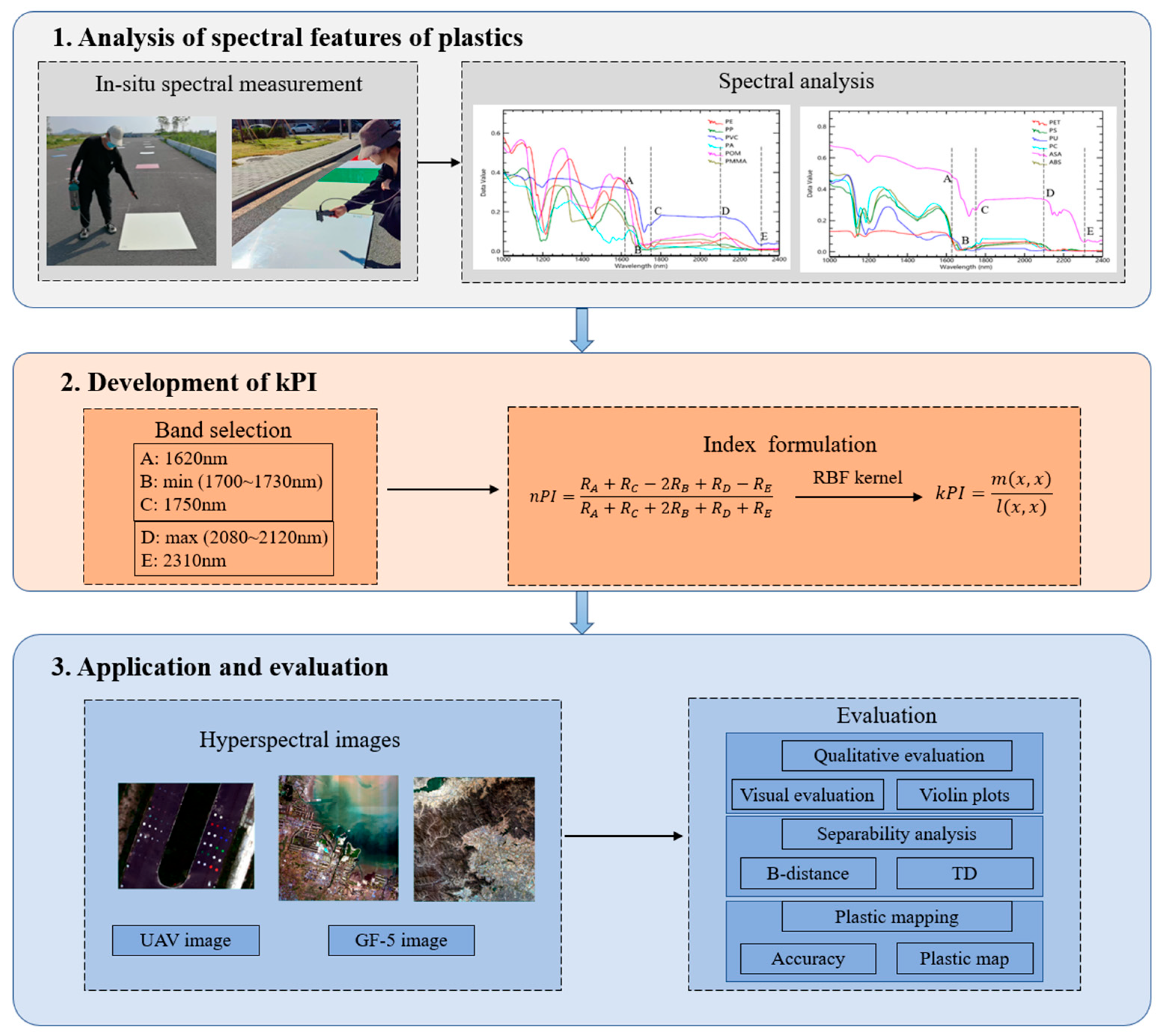
This study proposes a kernel-based plastic index specifically designed to enhance the mapping of plastics in urban built-up areas. The flowchart of the proposed index is shown in Figure 1.

First, in situ measured spectral data of 12 distinct plastic types with two chemical structures, aliphatic and aromatic plastics, were collected to characterize diagnostic absorption signatures. Next, for development of the kernel plastic index (kPI), the in situ measured spectral data were utilized to identify plastic-sensitive spectral bands. A linear normalized plastic index (nPI) was initially formulated based on absorption features, and the kernel method was then introduced to construct kPI from nPI. Finally, the proposed kPI was applied to both UAV and GF-5 hyperspectral datasets to evaluate its mapping performance.

2.1. Analysis of Spectral Features of Plastics

Since the plastics exhibit stable and diagnostic spectral characteristics in the SWIR range [31], SWIR spectral bands were selected for developing the plastic spectral index in this study. To analyze the absorption features of plastics in the SWIR range, this study first selected 12 plastic types for in situ spectral measurement. These plastics were categorized into two groups: aliphatic plastics without benzene rings and aromatic plastics containing benzene rings [24]. Specifically, six aliphatic plastics (polyethylene (PE), polypropylene (PP), polyvinylchloride (PVC), polymethyl methacrylate (PMMA), polyoxymethylene (POM), and polyamide (PA)) and six aromatic plastics (polyurethane (PU), polyethylene terephthalate (PET), acrylonitrile butadiene styrene (ABS), polystyrene (PS), polycarbonate (PC) and acrylonitrile styrene acrylate (ASA)) were chosen for investigation.

For each plastic type, 10 spectral measurements were collected and averaged to generate the representative spectral profile for that plastic type. Although the plastic samples exhibited various colors (including white, blue, red), the analyzed spectra focused on the near-infrared (NIR) to short-wave infrared (SWIR) range.

In situ spectral measurements were carried out in the Guangzhou and Beijing urban areas using the ASD FieldSpec4 field spectrometer (Analytical Spectral Devices, Inc., Boulder, CO, USA), which covers a wavelength range of 350–2500 nm. These samples were placed on concrete surfaces. All spectral measurements were conducted under clear weather and natural lighting conditions from 10:00 a.m. to 2:00 p.m. Reflectance calibration was performed using a white reference plate for each measurement. To ensure data quality, spectral bands affected by atmospheric water vapor absorption and sensor switching were removed from the obtained spectral data.

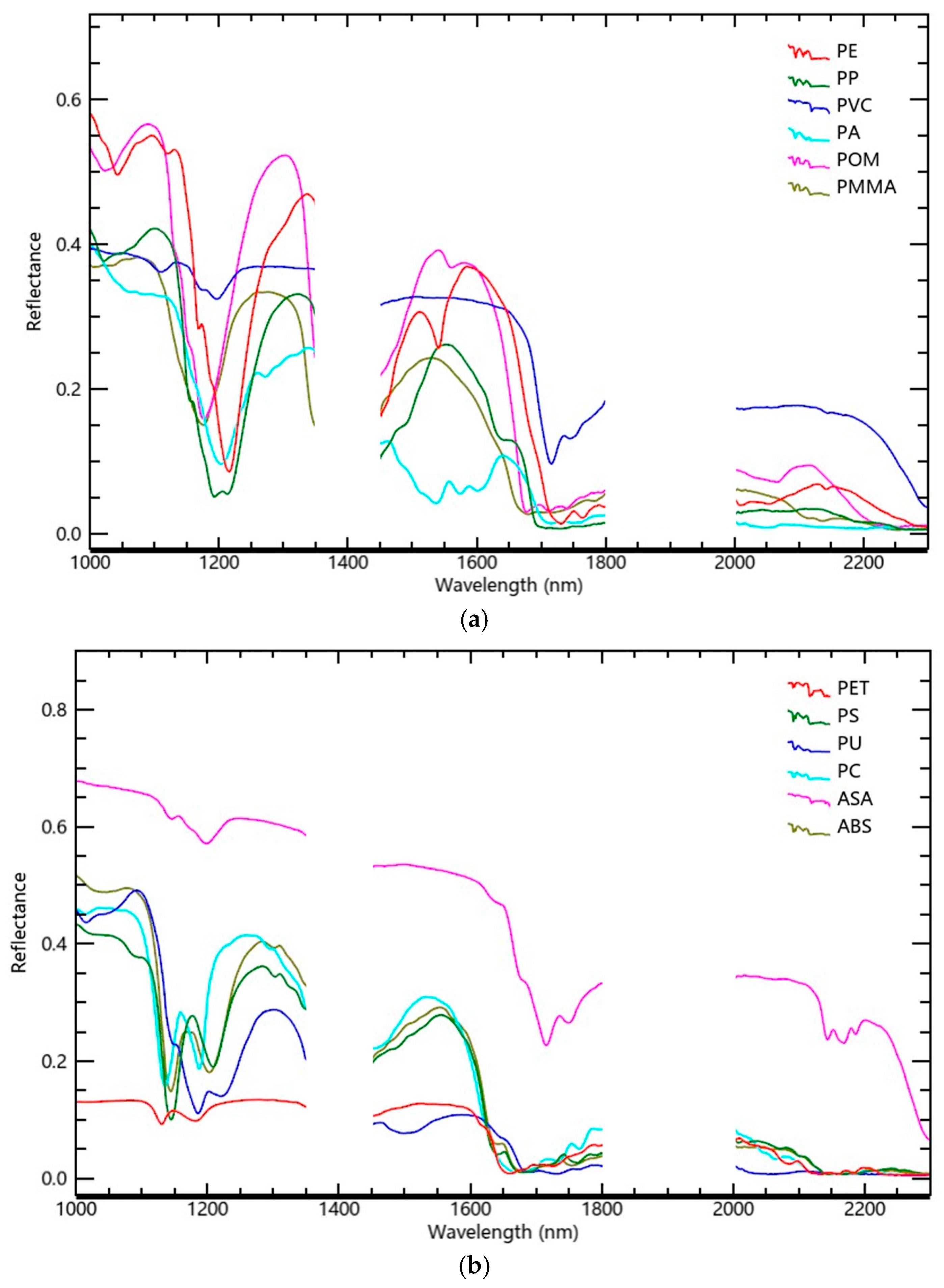
Figure 2 presents the measured spectral curves of aliphatic and aromatic plastics in the near-infrared to SWIR range (1000–2400 nm). As shown, the two categories exhibit markedly different absorption characteristics in the SWIR range.

For aliphatic plastics (Figure 2a), two major spectral features are observed in the SWIR region. In the 1600–1800 nm range, the reflectance begins to decline at 1620 nm, reaches a minimum between 1700 and 1730 nm, and then rises to a local peak at 1750 nm, forming a complete absorption trough. In the 2000–2400 nm range, reflectance decreases rapidly with increasing wavelength. A significant difference in reflectance is observed between the 2080–2120 nm range and 2310 nm; beyond 2310 nm, reflectance remains consistently low.

However, aromatic plastics (Figure 2b) exhibit slight differences from those of aliphatic plastics in the same wavelength range. In the 1600–1800 nm range, reflectance gradually decreases from 1620 nm, reaches a minimum in the 1680–1730 nm range, and then slowly rises to a local peak at 1750 nm. Notably, the absorption valley exhibits a slight shift toward shorter wavelengths relative to that of aliphatic plastics. In the 2000–2400 nm range, besides the differences in reflectance from the 2080–2120 nm range extending to 2310 nm, some aromatic plastics also exhibit an additional absorption feature near 2150 nm.

In summary, comparative spectral analysis of the two plastic types reveals two stable absorption features in the SWIR range. The first occurs in 1600–1800 nm, forming a full absorption trough flanked by a left shoulder at 1620 nm and a right shoulder at 1750 nm; the absorption trough falls at 1700 and 1730 nm, and the reflectance at the right shoulder is consistently lower than that at the left shoulder. The second feature occurs between 2000 and 2400 nm, where both plastic types exhibit a continuous decrease in reflectance with increasing wavelength. Specifically, reflectance steadily declines from the 2080–2120 nm range to 2310 nm, forming another stable and distinguishable spectral signature.

2.2. Development of the Kernel Plastic Index

Based on the spectral features outlined above, a normalized plastic index (nPI) is proposed by combining the absorption features at these two spectral regions. Specifically, the absorption depths at each location are calculated, and an initial plastic index is derived by combining the magnitudes of the absorption features in a normalized form. The depth of the first absorption feature (1600–1800 nm) is defined using the reflectance values at the left shoulder (A, 1620 nm), the trough core (B, minimum reflectance at 1700–1730 nm), and the right shoulder (C, 1750 nm) as follows: $\left({(R}_A+R_C)/2-R_B\right)$. The magnitude of the second absorption feature within the 2000–2400 nm range is defined as the reflectance difference between the reflectance peak (D, maximum reflectance at 2080–2120 nm) and the reflectance minimum (E, 2310 nm), expressed as ${(R}_D-R_E)$. In situ measured spectral features demonstrate that the first absorption feature (1600–1800 nm) represents the primary diagnostic signature for plastics, whereas the second absorption feature (2000–2400 nm) exhibits relatively weak absorption intensity for some plastic types. In addition, the first term contributes more substantially to distinguishing plastics from background land cover types. Therefore, assigning a higher relative weight to this more stable and discriminative feature is physically sound. To maintain consistency, this study applies a weighting factor of 2 to the first absorption feature, thereby balancing the reflectance difference between the shoulder and trough across the two absorption positions. The linearly normalized plastic index nPI is defined as

$$nPI={\displaystyle \frac{2\left(\frac{R_A+R_C}{2}-R_B\right)+(R_D-R_E)}{2\left(\frac{R_A+R_C}{2}+R_B\right)+\left(R_D+R_E\right)}},$$

(1)

By further simplifying Equation (1), we obtain the following expression:

$$nPI={\displaystyle \frac{R_A+R_C-2R_B+R_D-R_E}{R_A+R_C+2R_B+R_D+R_E}}.$$

(2)

However, as a linear band combination, the nPI cannot resolve complex nonlinear spectral relationships. Following the framework of kernel-based methods [32,33], a nonlinear mapping is applied to the nPI to enhance the spectral contrast between plastics and background land covers.

In this study, a Gaussian Radial Basis Function (RBF) kernel was selected to perform feature mapping, as it captures higher-order relationships between spectral bands and offers strong generalization [27]. The mapping function ϕ(x) and RBF kernel k (x, z) are defined as

$$\varphi \left(x\right)=\sqrt{{\displaystyle \frac{1}{m!{\sigma }^{2m}}}}{e}^{\left(-{\displaystyle \frac{x^2}{2{\sigma }^2}}\right)}{x}^m , m=0,1,2,3\dots \dots \infty$$

(3)

$$k\left(x,z\right)=\varphi {\left(x\right)}^T\varphi \left(z\right)=e^{\left(-{\displaystyle \frac{{\left|\left|x-z\right|\right|}^2}{2{\sigma }^2}}\right)},$$

(4)

where σ is the Gaussian RBF kernel width parameter, which directly determines the feature distribution of the high-dimensional mapping space and the model’s nonlinear fitting capability.

The construction of kPI is a methodological choice rather than a unique consequence of Equation (2). Following the formulation of kernelized normalized difference indices such as kNDVI and kNDMI [26,28], the numerator and denominator of nPI are mapped separately into an RKHS, and kPI is defined as the ratio of their squared norms. This design preserves the normalized-difference structure of nPI in the RKHS: the numerator norm $m\left(x,x\right)$ characterizes the nonlinear shoulder–trough absorption contrast, while the denominator norm $l\left(x,x\right)$ provides a reflectance energy-based normalization. The Gaussian RBF kernel implicitly maps reflectance into a high- or infinite-dimensional RKHS, allowing nonlinear spectral differences to be captured without specifying a polynomial order. This enhances the response to weak and asymmetric plastic absorption features. We note that this is not the unique possible kernelization. The present choice is motivated by its consistency with existing kernelized indices and its physical interpretability. To project both terms into the high-dimensional feature space, each individual band involved in the index calculation, such as $R_A\in R$, is projected into the Hilbert space $\mathcal{H}$ via the Gaussian RBF mapping to obtain its corresponding feature representation $\varphi \left(R_A\right)$. The inner product in this space defines the kernel function as $k\left(R_A,R_B\right)={<\varphi \left(R_A\right),\varphi \left(R_B\right)>}_{\mathcal{H}}$.

Subsequently, the numerator and denominator of the nPI formulation are projected into the Hilbert space $\mathcal{H}$, respectively. The feature mapping φ for the difference term in the numerator is as follows:

$$\begin{array}{l}\phi (x)=\phi \left(\left(R_A, R_B, R_C, R_D, R_E\right)\right)\\ =\varphi \left(R_A\right)+\varphi \left(R_C\right)-2\varphi \left(R_B\right)+\varphi \left(R_D\right)-\varphi \left(R_E\right)\in \mathcal{H}.\end{array}$$

(5)

The feature mapping $\psi$ for the summation term in the denominator is

$$\begin{array}{l}\psi (x)=\psi \left(\left(R_A, R_B, R_C, R_D, R_E\right)\right)\\ =\varphi \left(R_A\right)+\varphi \left(R_C\right)+2\varphi \left(R_B\right)+\varphi \left(R_D\right)+\varphi \left(R_E\right)\in \mathcal{H}.\end{array}$$

(6)

This study constructs the corresponding kernel function $m(·,·)$ based on the feature mapping $\phi$:

$$m(x_i,x_j)=<\phi (x_i),\phi (x_j){>}_{\mathcal{H}},$$

(7)

The squared norm of the multiband feature mapping $\phi$ in the high-dimensional space is calculated via the squared norm in the Hilbert space by $m\left(x,x\right)$:

$$\begin{array}{l}m(x,x)=m\left(\left(R_A, R_B, R_C, R_D, R_E\right),\left(R_A, R_B, R_C, R_D, R_E\right)\right)\\ =<\phi \left(\left(R_A, R_B, R_C, R_D, R_E\right)\right),\phi \left(\left(R_A, R_B, R_C, R_D, R_E\right)\right){>}_{\mathcal{H}}.\end{array}$$

(8)

The function $m\left(x,x\right)$ represents the magnitude of nonlinear differences in the absorption features of plastics in high-dimensional space.

Similarly, we construct a corresponding kernel function $l (·,·)$ based on the mapping $\psi$ to represent the sum terms in the denominator:

$$\begin{array}{l}l(x,x)=l\left(\left(R_A, R_B, R_C, R_D, R_E\right),\left(R_A, R_B, R_C, R_D, R_E\right)\right)\\ =<\psi \left(\left(R_A, R_B, R_C, R_D, R_E\right)\right),\psi \left(\left(R_A, R_B, R_C, R_D, R_E\right)\right){>}_{\mathcal{H}}.\end{array}$$

(9)

Therefore, through the kernel formulation, the nPI is defined in Hilbert space as the ratio of the numerator difference function m to the sum function l. The form of kPI is

$$kPI={\displaystyle \frac{m(x,x)}{l(x,x)}}={\displaystyle \frac{m\left(\left(R_A, R_B, R_C, R_D, R_E\right),\left(R_A, R_B, R_C, R_D, R_E\right)\right)}{l\left(\left(R_A, R_B, R_C, R_D, R_E\right),\left(R_A, R_B, R_C, R_D, R_E\right)\right)}}.$$

(10)

The validity of kPI requires m and l to be symmetric and positive semi-definite. Symmetry is inherently satisfied by Equations (8) and (9). The positive semi-definite condition requires that, for any positive integer N, any samples $x_1,x_2,\dots ,x_N\in X$, and any non-zero column vector $\mathsf{\alpha }=({\alpha }_1,{\alpha }_2,\dots ,{\alpha }_N)\in R^N$, the Gram matrix $G_{ij}=k(x_i,x_j)$ constructed from the kernel function must satisfy the non-negativity of the quadratic form:

$${\alpha }^{T}G\alpha \ge 0.$$

(11)

Based on the inner product definition of the kernel function m, its quadratic form can be explicitly expressed as the squared norm in the high-dimensional space, that is

$$\begin{array}{l}{\alpha }^T{G}_m\alpha ={\displaystyle \sum _{i=1}^N{\displaystyle \sum _{j=1}^N{\alpha }_i}}{\alpha }_j•m\left(x_i,x_j\right)\\ ={\displaystyle \sum _{i=1}^N{\displaystyle \sum _{j=1}^N{\alpha }_i}}{\alpha }_j{〈\phi \left(x_i\right),\phi \left(x_j\right)〉}_{\mathcal{H}}={\left|\left|{\displaystyle \sum _{i=1}^N{\alpha }_i}\phi \left(x_i\right)\right|\right|}_{\mathcal{H}}^2\\ =\left|\right|{\displaystyle \sum _{i=1}^N{\alpha }_i}\left(\varphi \left(R_{Ai}\right)+\varphi \left(R_{Ci}\right)-2\varphi \left(R_{Bi}\right)+\varphi \left(R_{Di}\right)-\varphi \left(R_{Ei}\right)\right)|{|}_{\mathcal{H}}^2\ge 0.\end{array}$$

(12)

The kernel functions m and l are both positive semi-definite and valid kernel functions. Meanwhile, because kPI is implemented as a scalar spectral index rather than as a kernel matrix within machine learning kernel algorithms, the ratio m/l is not required to satisfy Mercer’s kernel conditions. The primary purpose of establishing that m and l are valid positive semi-definite kernels is to guarantee the mathematical legitimacy of the mapping into RKHS, thereby confirming that the squared norms mapped by m and l in the high-dimensional space are well-defined and mathematically meaningful. Furthermore, in the Gaussian RBF kernel, where $k\left(R_i,R_i\right)=1$, the difference term function m is expressed as

$$\begin{array}{l}m\left(\left(R_A, R_B, R_C, R_D, R_E\right),\left(R_A, R_B, R_C, R_D, R_E\right)\right)\\ =k\left(R_A,R_A\right)+2k\left(R_A,R_C\right)-4k\left(R_A,R_B\right)+2k\left(R_A,R_D\right)\\ -2k\left(R_A,R_E\right)+k\left(R_C,R_C\right)-4k\left(R_B,R_C\right)+2k\left(R_C,R_D\right)\\ -2k\left(R_C,R_E\right)+4k\left(R_B,R_B\right)-4k\left(R_B,R_D\right)+4k\left(R_B,R_E\right)\\ +k\left(R_D,R_D\right)-2k\left(R_D,R_E\right)+k\left(R_E,R_E\right)\\ =2\left(\begin{array}{l}4+k\left(R_A,R_C\right)+k\left(R_A,R_D\right)+k\left(R_C,R_D\right)+2k\left(R_B,R_E\right)\\ -2k\left(R_A,R_B\right)-2k\left(R_B,R_C\right)-2k\left(R_B,R_D\right)\\ -k\left(R_A,R_E\right)-k\left(R_C,R_E\right)-k\left(R_D,R_E\right)\end{array}\right).\end{array}$$

(13)

The summation function l is expressed as

$$\begin{array}{l}l\left(\left(R_A, R_B, R_C, R_D, R_E\right),\left(R_A, R_B, R_C, R_D, R_E\right)\right)\\ =2\left(\begin{array}{l}4+k\left(R_A,R_C\right)+k\left(R_A,R_D\right)+k\left(R_C,R_D\right)+2k\left(R_B,R_E\right)\\ +2k\left(R_A,R_B\right)+2k\left(R_B,R_C\right)+2k\left(R_B,R_D\right)\\ +k\left(R_A,R_E\right)+k\left(R_C,R_E\right)+k(R_D,R_E)\end{array}\right).\end{array}$$

(14)

Therefore, the kernel plastic index (kPI) based on Gaussian RBF kernel is expressed as follows:

$$\begin{array}{l}kPI={\displaystyle \frac{m\left(\left(R_A, R_B, R_C, R_D, R_E\right),\left(R_A, R_B, R_C, R_D, R_E\right)\right)}{l\left(\left(R_A, R_B, R_C, R_D, R_E\right),\left(R_A, R_B, R_C, R_D, R_E\right)\right)}}\\ ={\displaystyle \frac{\left(\begin{array}{l}4+k\left(R_A,R_C\right)+k\left(R_A,R_D\right)+k\left(R_C,R_D\right)+2k\left(R_B,R_E\right)\\ -2k\left(R_A,R_B\right)-2k\left(R_B,R_C\right)-2k\left(R_B,R_D\right)\\ -k\left(R_A,R_E\right)-k\left(R_C,R_E\right)-k\left(R_D,R_E\right)\end{array}\right)}{\left(\begin{array}{l}4+k\left(R_A,R_C\right)+k\left(R_A,R_D\right)+k\left(R_C,R_D\right)+2k\left(R_B,R_E\right)\\ +2k\left(R_A,R_B\right)+2k\left(R_B,R_C\right)+2k\left(R_B,R_D\right)\\ +k\left(R_A,R_E\right)+k\left(R_C,R_E\right)+k\left(R_D,R_E\right)\end{array}\right)}}.\end{array}$$

(15)

where

$$k\left(R_i,R_j\right)=e^{(-{\displaystyle \frac{{‖R_i-R_j‖}^2}{2{\sigma }^2}})},$$

(16)

where σ is the Gaussian RBF kernel width parameter, which controls the scale of the nonlinear feature mapping.

The kernel width parameter σ can be determined via fixed parameter method, adaptive method, maximum method, and maximum difference method [28]. In this study, the maximum method was used for parameter selection, which involves combining the average reflectance of each pixel across all bands with a fixed parameter; for each pixel,

$$\sigma =\max \left({\displaystyle \frac{R_A+R_C+2R_B+R_D+R_E}{6}}, 0.1\right),$$

(17)

where A (1620 nm), C (1750 nm), and E (2310 nm) are fixed bands, while B (minimum reflectance at 1700–1730 nm) and D (maximum reflectance at 2080–2120 nm) are interval bands.

It should be clarified that there is a fundamental difference in the operational domain between the kernel operation of kPI and that of conventional kernel learning methods. In traditional machine learning, kernel functions (such as in Support Vector Machines) are employed to construct a global Gram matrix across spatial samples, where a sample-dependent kernel width would inevitably compromise the global symmetry and positive semi-definiteness of the matrix. In contrast, the kernel operation in kPI is strictly confined to the different spectral bands within an individual pixel, without constructing any global kernel matrix across spatial pixels. For any given pixel p, its adaptive bandwidth ${\sigma }_p$ is a deterministic positive scalar. Consequently, the local Gram matrix formed by the five spectral bands within that pixel strictly preserves real symmetry and positive semi-definiteness.

Following the maximum method, this study couples a pixel-wise adaptive mean reflectance with a fixed lower bound constant n: on the one hand, the mean band reflectance characterizes the radiant energy level of the local surface, allowing ${\sigma }_p$ to adjust dynamically from pixel to pixel and thereby achieve adaptive dynamic contrast stretching; on the other hand, the threshold n = 0.1 provides a truncation boundary, effectively preventing numerical instability over low-reflectance targets (such as water bodies and shadows) where σ approaching zero would otherwise cause severe anomalies.

2.3. Evaluation of the Proposed Index

To assess the performance of kPI, this study evaluates its effectiveness from three perspectives: qualitative analysis, separability evaluation, and plastic mapping. kPI is compared with three existing plastic spectral indices and a one-class classification method to validate its performance. Furthermore, a combined plastic index, which also utilizes two distinct absorption features of plastics, is developed for further validation.

2.3.1. Evaluation Methods

Qualitative Evaluation

Through visual evaluation, this study compares the performance of kPI with that of the comparative indices across different study areas. Additionally, violin plots are used to compare the statistical distributions in index values among different land cover types.

Separability Evaluation

This study uses two separability metrics to evaluate the separability between plastic and other land covers: Transformed Divergence (TD) [34,35] and Bhattacharyya distance (B-distance) [36].

Transformed Divergence (TD) measures class separability on a saturated scale from 0 to 2, where values above 1.9, between 1.7 and 1.9, and below 1.7 indicate high, moderate, and poor separability, respectively [34]. The B-distance measures the statistical distance between two Gaussian distributions, with larger B-distance values indicating better separability.

Plastic Mapping

This study employs a thresholding method to perform plastic mapping on plastic spectral index images. This study employs Monte Carlo cross-validation (MCCV) [37] to determine the optimal threshold. Specifically, 30% of the reference samples were allocated for threshold optimization, leaving 70% for independent accuracy assessment. Over 100 random trials on this optimization subset, samples were partitioned into training (75%) and validation (25%) data. Candidate thresholds were iteratively evaluated on the training sets, and the threshold yielding the highest average F1-score on validation data across the 100 iterations was selected as optimal.

After obtaining the plastic mapping results using the optimal threshold, visual evaluation and accuracy assessment are conducted. For accuracy evaluation, a confusion matrix is used to calculate overall accuracy (OA), producer’s accuracy (PA), user’s accuracy (UA), and the F1 score.

2.3.2. Comparative Methods

Development of a Combined Plastic Index (cPI) for Comparison

To validate the effectiveness of kPI, this study constructs a combined plastic index (cPI) that also integrates two absorption features, using the same five bands as those used for kPI.

First, the absorption depth at the first absorption feature (between 1600 and 1800 nm) is defined as ${PI}_1$:

$$P{I}_1=\left({\lambda }_B-{\lambda }_A\right){\displaystyle \frac{R_C-R_A}{{\lambda }_C-{\lambda }_A}}+R_A-R_B,$$

(18)

where the definitions of bands A–C are identical to those in Section 2.2, λ_A, λ_B, and λ_c are spectral wavelengths of bands A, B and C.

Next, the normalized reflectance difference between D and E quantifies the second feature in 2000–2400 nm as ${PI}_2$:

$$P{I}_2={\displaystyle \frac{R_D-R_E}{R_D+R_E}},$$

(19)

where the definitions of bands D and E are identical to those in Section 2.2.

To enhance the second absorption feature, this study adopts arctan (5PI₂) as an enhancement function to increase sensitivity to low values of ${PI}_2$. A constant of 1 is added after the enhancement function to ensure non-negativity, resulting in the term (1 + arctan (5PI₂)).

The two terms described above are then combined multiplicatively to yield the final cPI expression as follows:

$$cPI=P{I}_1\left(1+\arctan \left(5P{I}_2\right)\right),$$

(20)

Existing Plastic Spectral Indices

This study selected three existing plastic spectral indices for comparison, including the Hydrocarbon Index (HI) [22], the Normalized Hydrocarbon Index (nHI) [23], and the Normalized Difference Plastic Index (NDPI) [20].

Plastic Mapping Using the Improved One-Class Random Forest

To further validate kPI, this study selected a one-class classification method, the improved one-class random forest (iOCRF) [38], as a comparison method. Unlike traditional one-class random forests that rely on simulated pseudo-backgrounds [39], iOCRF directly samples non-target instances from unlabeled data, thereby capturing more accurate background distributions [38]. In this study, iOCRF performs classification using manually selected plastic targets and automatically extracted non-plastics background samples.

The classification method was based on all spectral bands within the 1600–1800 nm and 2000–2400 nm ranges, which are sensitive to the diagnostic absorption features of plastics and consistent with those used in the proposed kPI. The model parameters were set as follows: the number of trees to 200, the maximum tree depth to 10, and the number of split features to one plus the square root of the number of bands [38,39]. In each study area, approximately 20% of the plastic samples were randomly selected for model training to generate the final plastic mapping results.

3. Study Areas and Data

To validate the effectiveness of kPI in different scenarios, three study areas were selected in Guangzhou, Weifang, and Beijing, China.

3.1. Guangzhou Area and Data

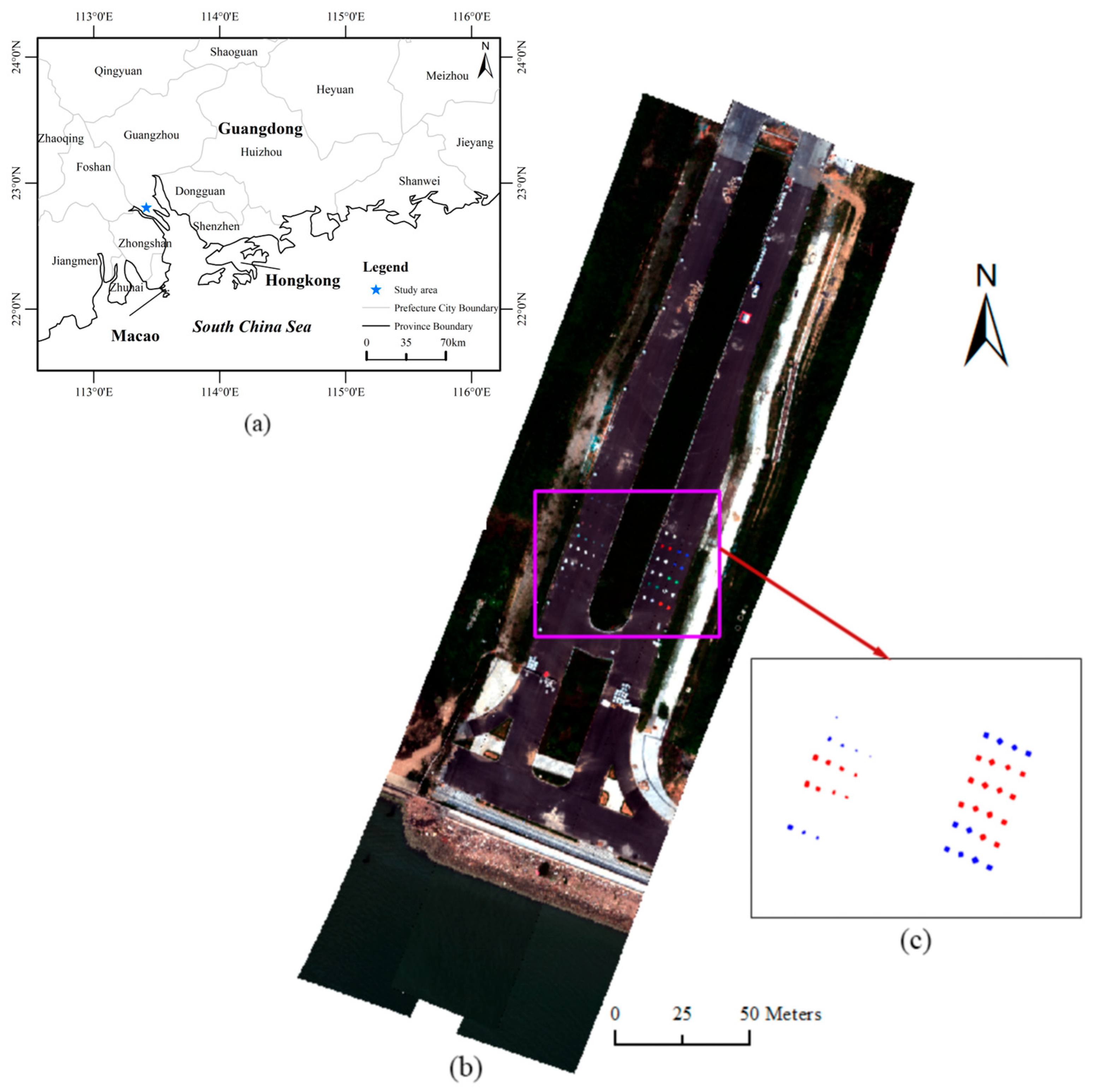
The Guangzhou study area is located in Caifen, Nansha District, Guangzhou City, Guangdong Province (Figure 3a). Land cover types in the area include natural features (bare soil, vegetation, and water) and artificial features (concrete road and brick road). Plastic materials present in the area include artificially placed plastic sheets and plastic bottles, covering the two major categories of aliphatic and aromatic plastics as previously illustrated [24].

Specifically, to investigate the spectral characteristics of typical plastic materials, samples of virgin (unused) plastics were laid out in the area (Figure 3b). These samples were arranged into two sections; in the right section, the area contained plastic plates: 24 plates representing 12 different plastic compositions (Figure 3b). Each plastic plate measured 1 m × 1 m × 5 mm and belonged to one of two chemical structures: aliphatic plastics or aromatic plastics. Within each type of plastic (aliphatic or aromatic), six specific plastic types were represented. The aliphatic plastics included PE, PP, PVC, PA, PMMA, and POM. The aromatic plastics included ABS, PS, PC, PU, ASA and PET. Two replicate sheets were used for each plastic composition.

In the left section, plastic bags and plastic bottles were arranged in clusters of different sizes (Figure 3b), resulting in pronounced intra-cluster spectral heterogeneity and weaker spatial autocorrelation. This contrast indicates that the degree of spatial autocorrelation is not uniform across the UAV dataset. Hyperspectral data used were acquired in September 2021 using a DJI M600 PRO UAV (SZ DJI Technology Co.,Ltd., Shenzhen, China), with a spectral resolution of 2.216 nm (VNIR, 400–1002 nm), and 5.974 nm (SWIR, 1002–2513 nm) and a spatial resolution of 0.07 m. Following preliminary screening, 456 bands were retained.

After preprocessing, high-quality reflectance data were obtained (Figure 3b). The UAV hyperspectral image has dimensions of 982 × 772 pixels, with the corresponding plastic distribution shown in Figure 3c, where the aliphatic and aromatic plastic samples comprise 4793 and 3138 pixels, respectively.

3.2. Weifang Area and Data

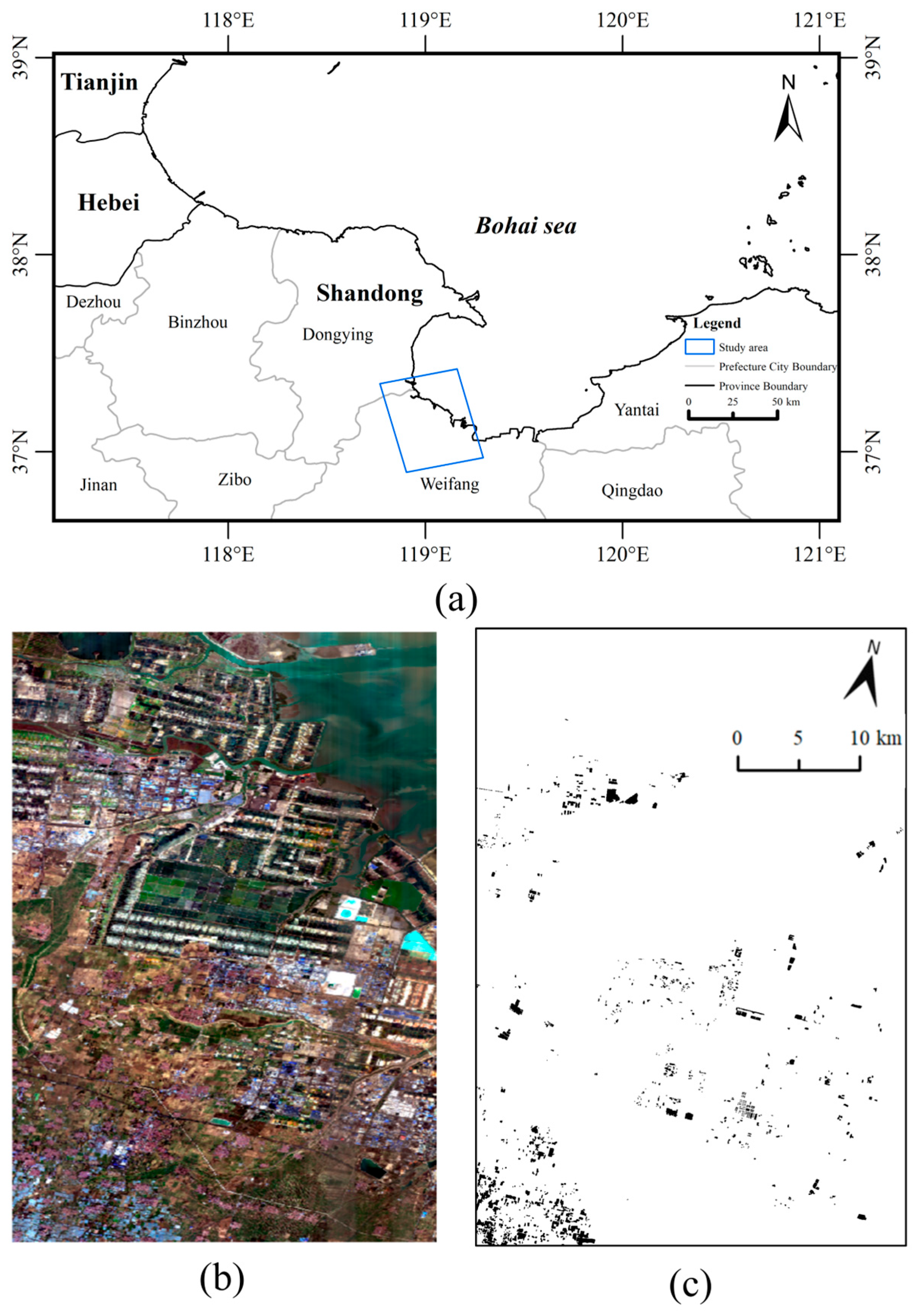
The Weifang study area spans northern Weifang City and southern Dongying, Shandong Province (Figure 4a). Major land cover types in the area include villages, towns, farmland, seawater, as well as inland aquaculture ponds and salt fields. Plastics include plastic greenhouses, photovoltaic panels containing plastic materials in industrial parks, and plastic roofing in villages and towns [40].

The hyperspectral data used in this study were obtained from the GF-5 on 14 November 2019, by the Advanced Hyperspectral Imager. The data include 330 spectral bands within the spectral range of 400–2500 nm, including 150 VNIR bands and 180 SWIR bands with a swath width of 60 km and a spatial resolution of 30 m.

The GF-5 hyperspectral data were preprocessed according to previous studies [41,42,43]. The resulting image, comprising 1202 × 1726 pixels was used for subsequent analysis (Figure 4b).

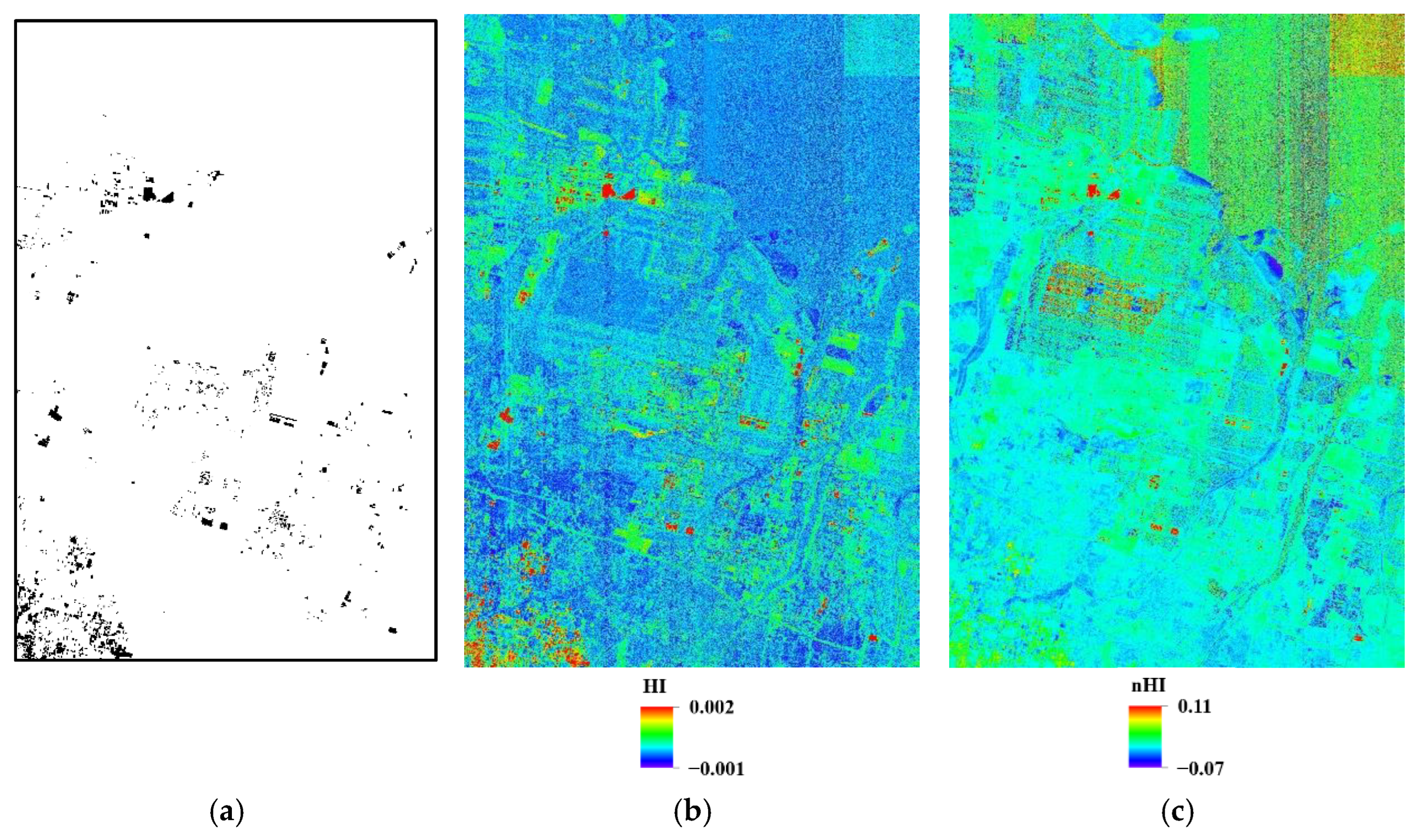
The study area was visually interpreted using high-resolution imagery, and plastic distribution was manually annotated. A total of 35,480 plastic pixels were selected, with their distribution shown in Figure 4c.

3.3. Beijing Area and Data

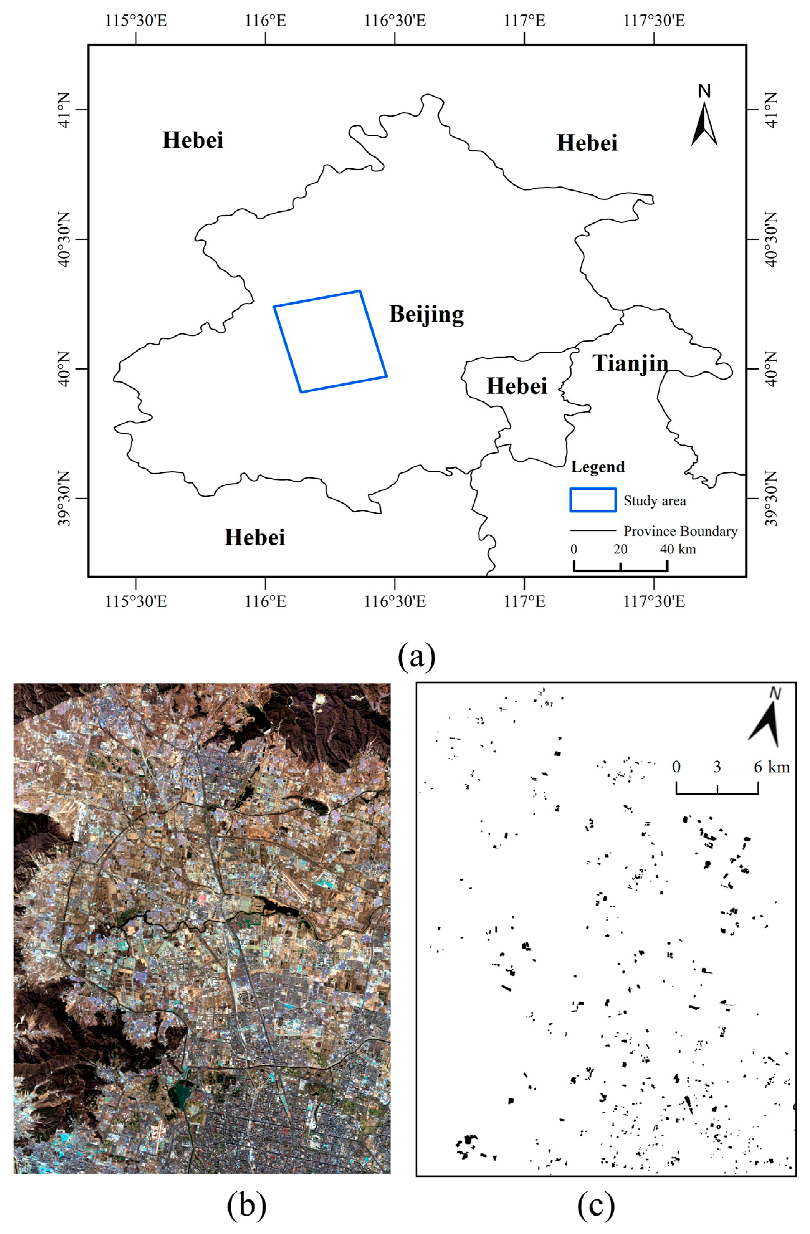
The study area in Beijing is located in the northern part of the city, mainly covering Haidian District and Changping District (Figure 5a). This area is a typical urban built-up area with various land cover types, such as vegetation, water bodies, bare soil, buildings, municipal road, and other artificial impervious surfaces. The main plastic targets include artificial turf on sports fields, plastic surfaces in parks and sports venues, building roofs made of polymer materials, and green plastic covers at construction sites.

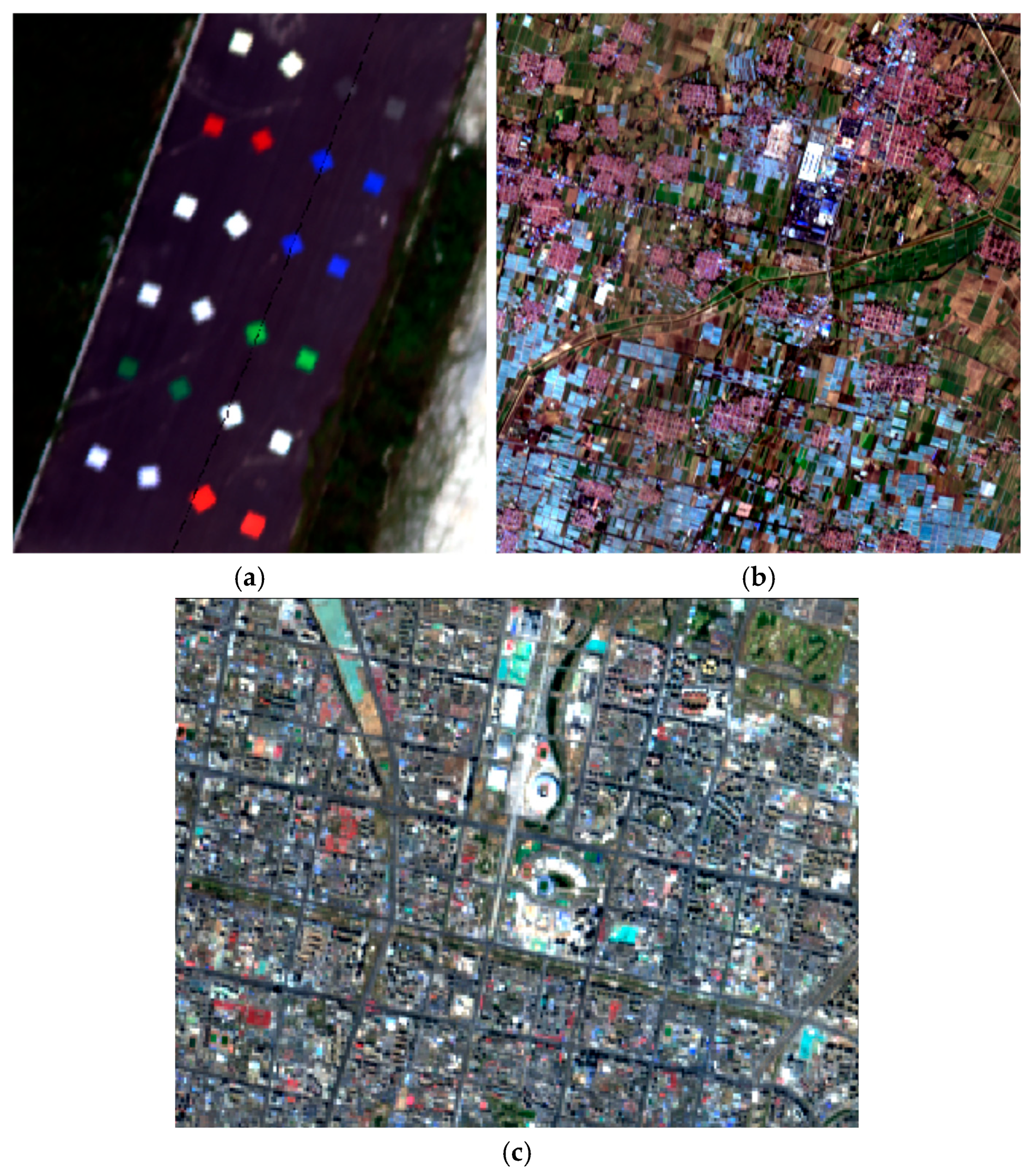
The Beijing area was covered by GF-5 hyperspectral data acquired on 25 March 2019, preprocessed identically to the Weifang dataset. The final image size for the area is 970 × 1300 pixels (Figure 5b).

Through visual interpretation, a total of 18,240 plastic sample pixels (Figure 5c) and 86,312 non-plastic sample pixels were selected from the study area.

4. Experimental Results

4.1. Experimental Results for the Guangzhou Area

4.1.1. Qualitative Evaluation

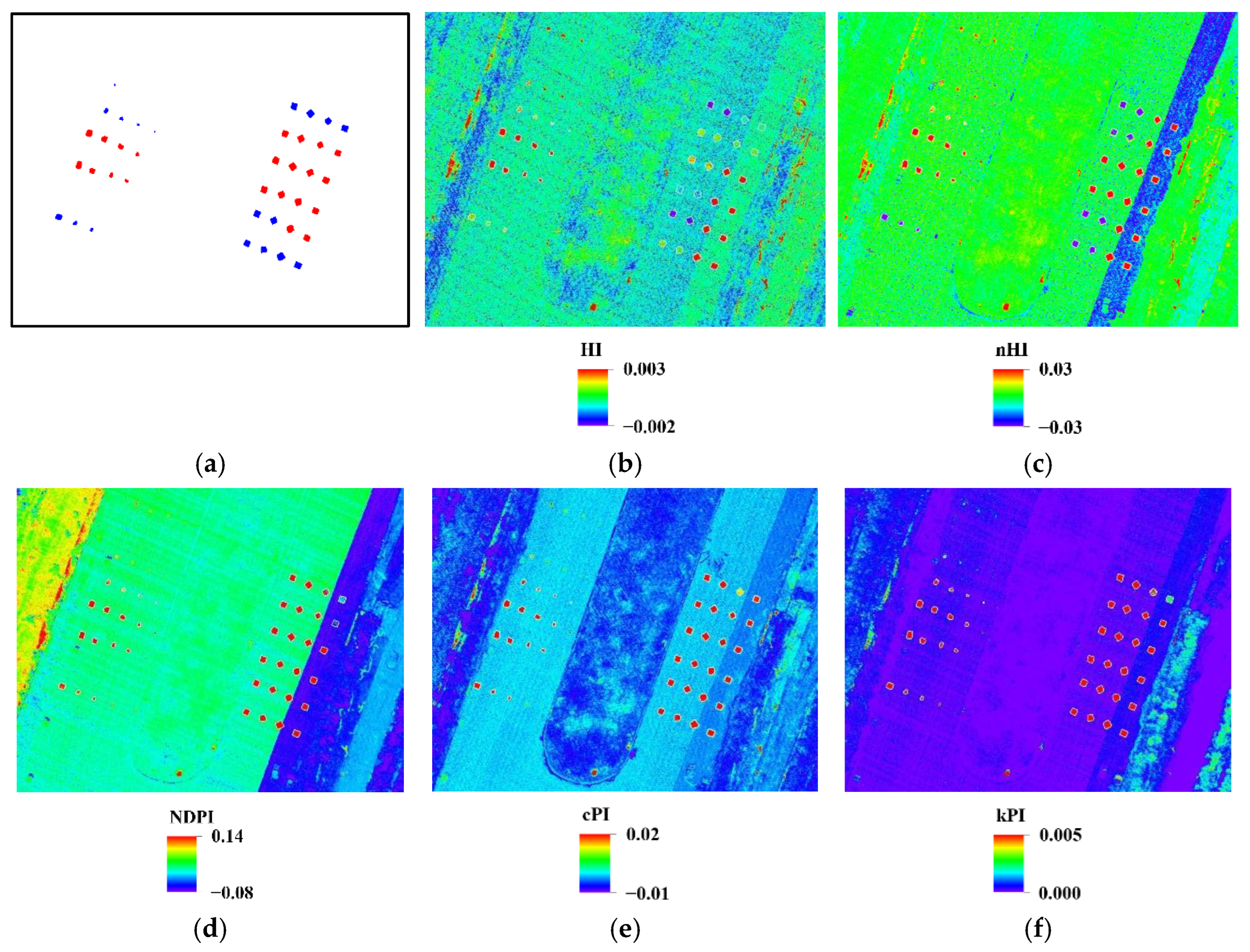
Figure 6 presents the spectral index images for the Guangzhou area, with Figure 6a showing the reference plastic distribution. In the HI (Figure 6b) and nHI (Figure 6c) images, only aliphatic plastics exhibited high index values (appeared red), whereas aromatic plastics showed lower indices, similar to the surrounding non-plastic materials. The NDPI image (Figure 6d) better highlighted plastic areas but also produced high index values (appearing red and yellow) in the soil regions on the left. The cPI image (Figure 6e) showed performance even higher, although a few soil areas still exhibited relatively high values. The kPI image (Figure 6f) performed best: all plastic regions exhibited high values and all non-plastic background areas were suppressed (appearing blue–purple).

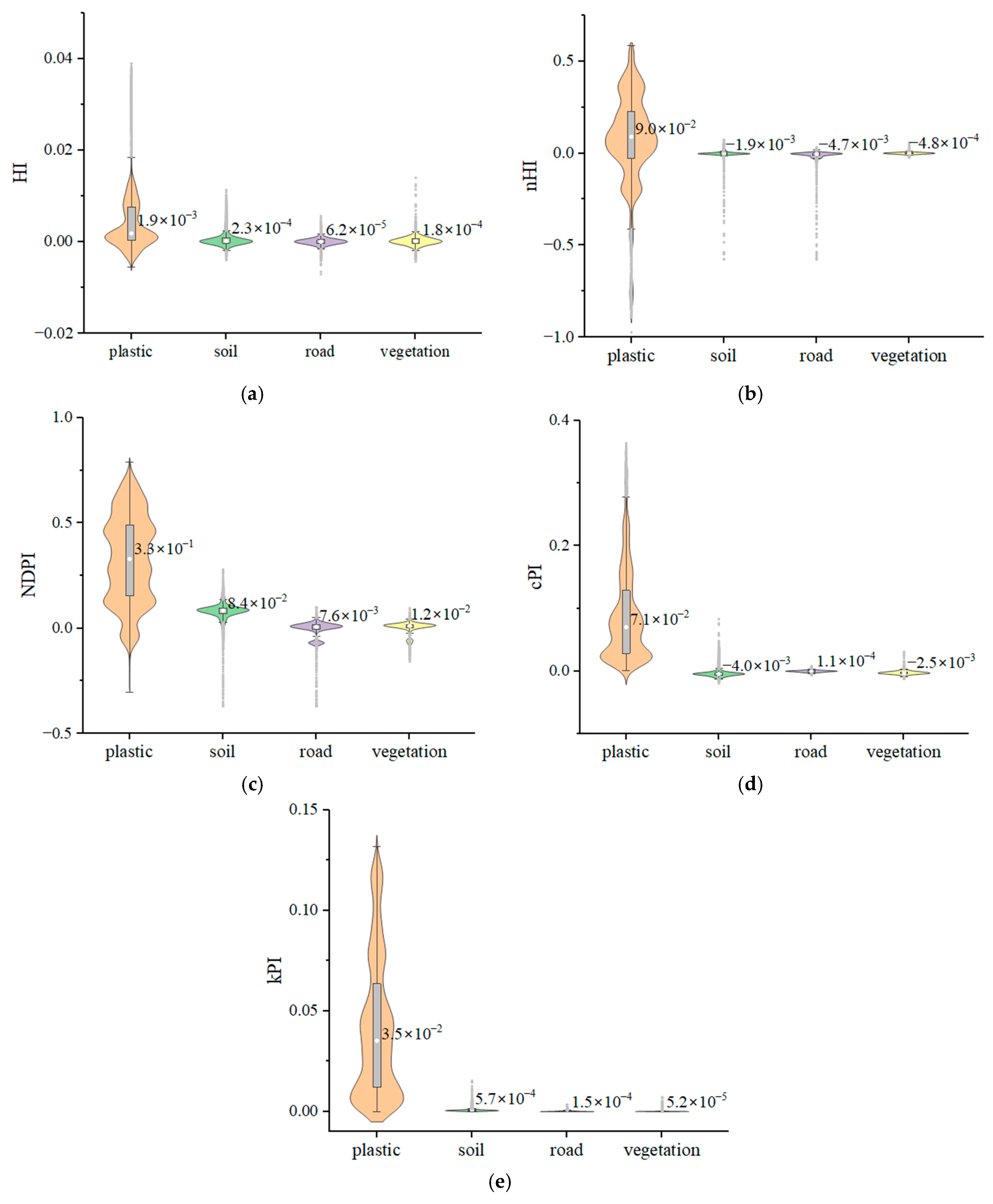
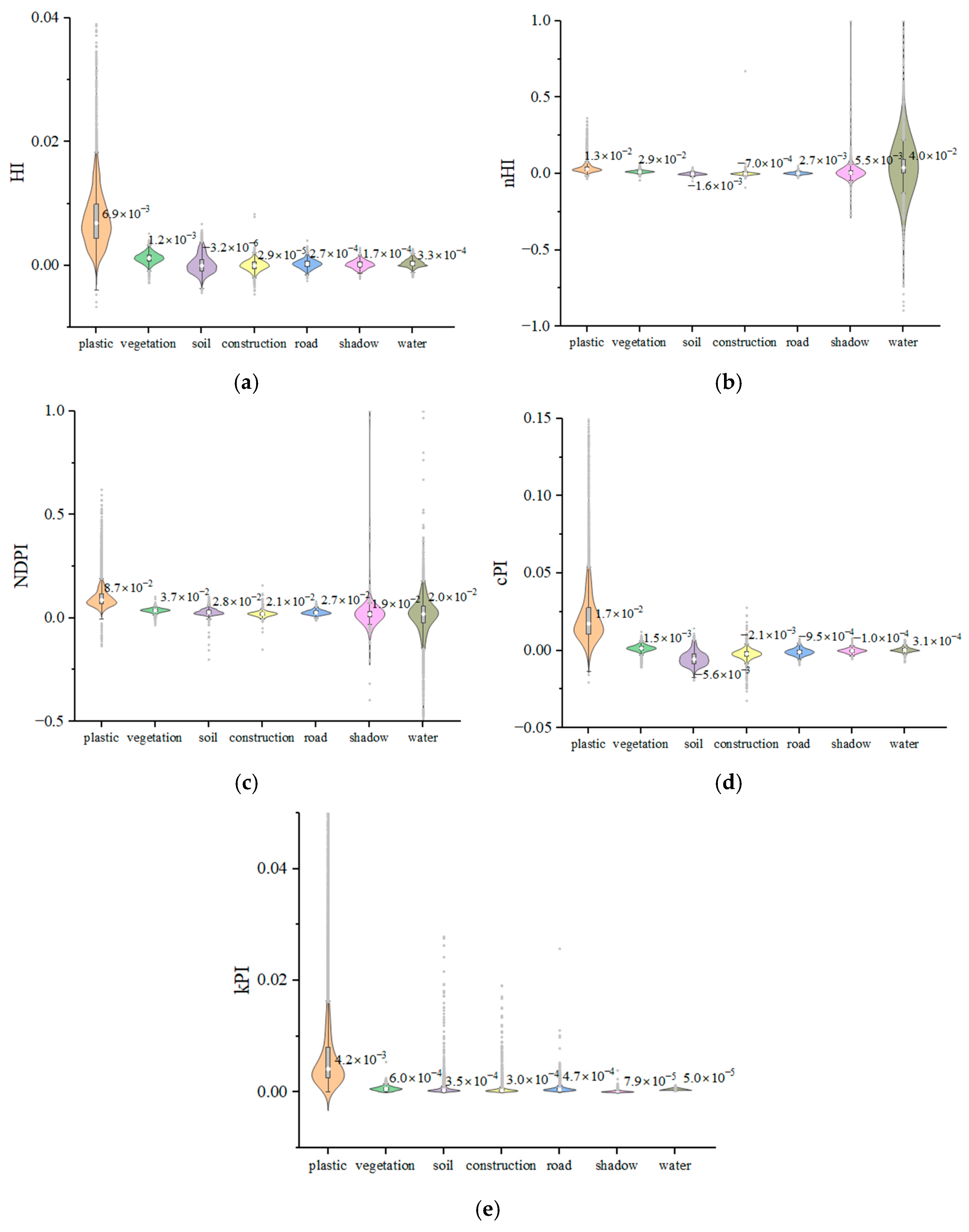
Figure 7 presents the violin plots of the spectral indices in the Guangzhou area. For the HI and nHI (Figure 7a,b), the value ranges for plastics and non-plastics showed significant overlap making the separation of the two difficult. The NDPI (Figure 7c) exhibited relatively high values for soil, which overlapped with the interquartile range for plastics and could easily lead to confusion. Plastic samples generally had high values for the cPI (Figure 7d), resulting in good separability from background land covers. For the kPI (Figure 7e), non-plastic values were highly concentrated and significantly lower than plastic values. kPI provided the most distinct separability.

4.1.2. Separability Analysis

Table 1. Separability metrics between plastics and background land covers in the Guangzhou area.

	Land Cover Type	HI	nHI	NDPI	cPI	kPI
TD	Soil	1.79	2	1.96	2	2
	Road	2	2	2	2	2
	Vegetation	2	2	2	2	2
B-distance	Soil	0.58	0.96	0.83	1.25	1.91
	Road	0.94	0.98	1.19	1.99	2.61
	Vegetation	0.83	1.66	1.26	1.75	2.12

presents the separability metrics in the Guangzhou area. For the TD metrics, only HI showed a value below 1.9 between plastic and soil, while other indices reached or approached 2.0. For the B-distance metrics, most values for HI, nHI, and NDPI were less than 1.5, whereas cPI yielded values between 1 and 2. kPI outperformed all other indices, with most B-distances exceeding 2.0, effectively improving plastics discrimination.

4.1.3. Plastic Mapping Results

Table 2. Accuracies for plastic mapping with different methods in the Guangzhou area.

Method	Threshold	F1 (%)	OA (%)	PA (%)	UA (%)
HI	0.0048	43.6	99.0	34.6	59.1
nHI	0.047	70.8	99.5	59.4	87.6
NDPI	0.17	81.4	99.6	72.6	92.6
iOCRF		52.7	99.0	53.9	51.5
cPI	0.019	85.8	99.7	87.9	83.7
kPI	0.0055	89.6	99.8	85.9	93.6

Note: OA: overall accuracy; PA: plastics producer’s accuracy; UA: plastics user’s accuracy.

presents the mapping accuracies in the Guangzhou area. HI, nHI, and iOCRF yielded low F1-scores below 80%, with HI recording the lowest at 43.6%. While nHI and NDPI achieved high UAs over 80%, their PAs remained limited to under 60% for nHI. In contrast, NDPI and cPI attained higher F1-scores of 81.4% and 85.8%, with cPI maintaining balanced UA and PA above 80%. kPI achieved the highest overall performance, attaining an F1-score of 89.6%, delivering balanced PA and UA over 85% but also achieved the highest UA at 93.6%, minimizing both omission and commission errors.

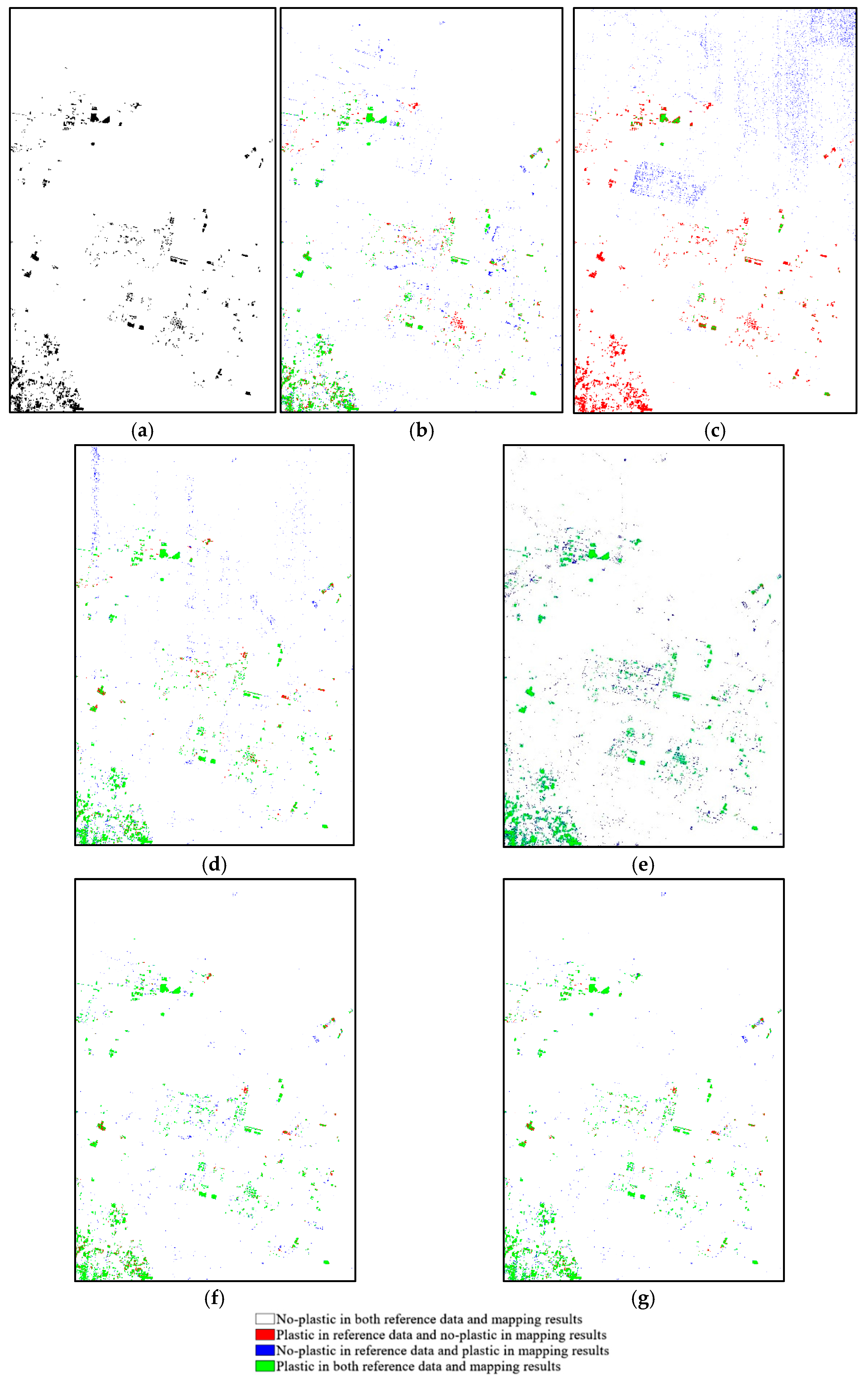
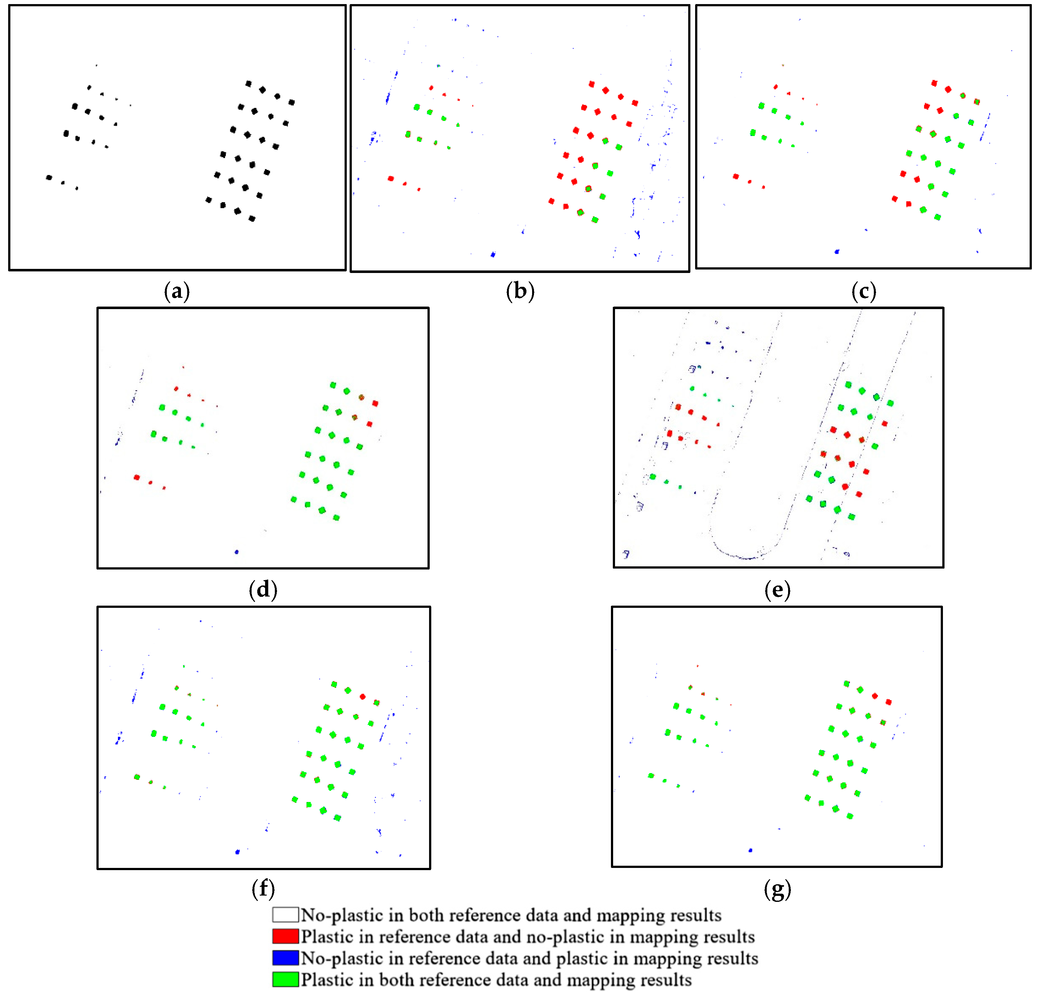
The plastic mapping results obtained using different methods are shown in Figure 8. The mapping results using HI, nHI, and iOCRF all exhibited significant omissions of plastics, with a large number of plastic pixels remaining unrecognized (Figure 8b,c,e). In the results using NDPI (Figure 8d), some plastics were still omitted, and certain soil areas on the left side were incorrectly classified as plastics. cPI (Figure 8f) showed that a large number of non-plastic pixels were misclassified as plastic. In contrast, kPI (Figure 8g) produced fewer misclassified and omitted pixels against the competing methods, which confirmed its best overall performance.

4.2. Weifang Area

4.2.1. Qualitative Evaluation

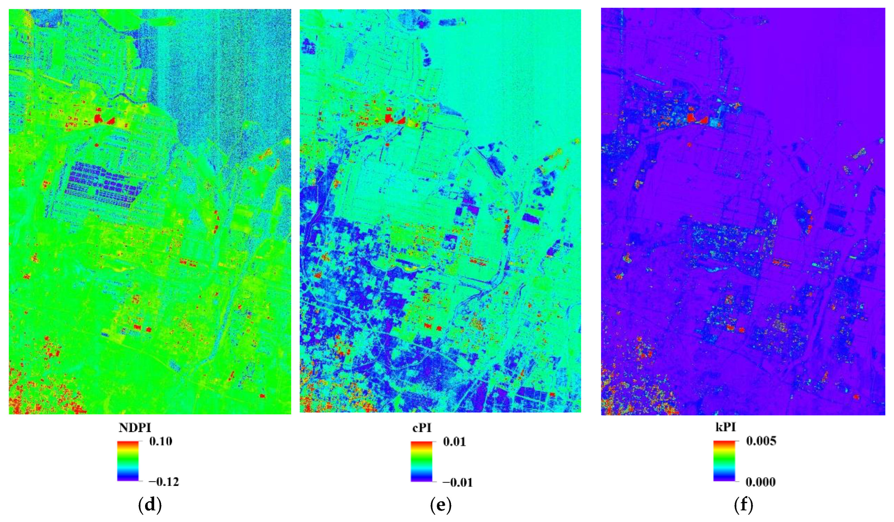
Figure 9 presents spectral index images for the Weifang area. In the HI image (Figure 9b), although the plastic-covered areas exhibited high values, numerous high-value pixels also appeared in non-plastic areas, introducing notable noise. In the nHI image (Figure 9c), plastic greenhouses in the lower-left corner showed low values (yellow–green), making them difficult to distinguish from the background. Both the NDPI (Figure 9d) and HI image showed prominent values over the water body in the upper-right corner, which could easily be confused with plastics. In contrast, the cPI and kPI images (Figure 9e,f) both displayed high index values over plastic areas. By suppressing non-plastic pixels, kPI provided the best separation between plastic and background land covers.

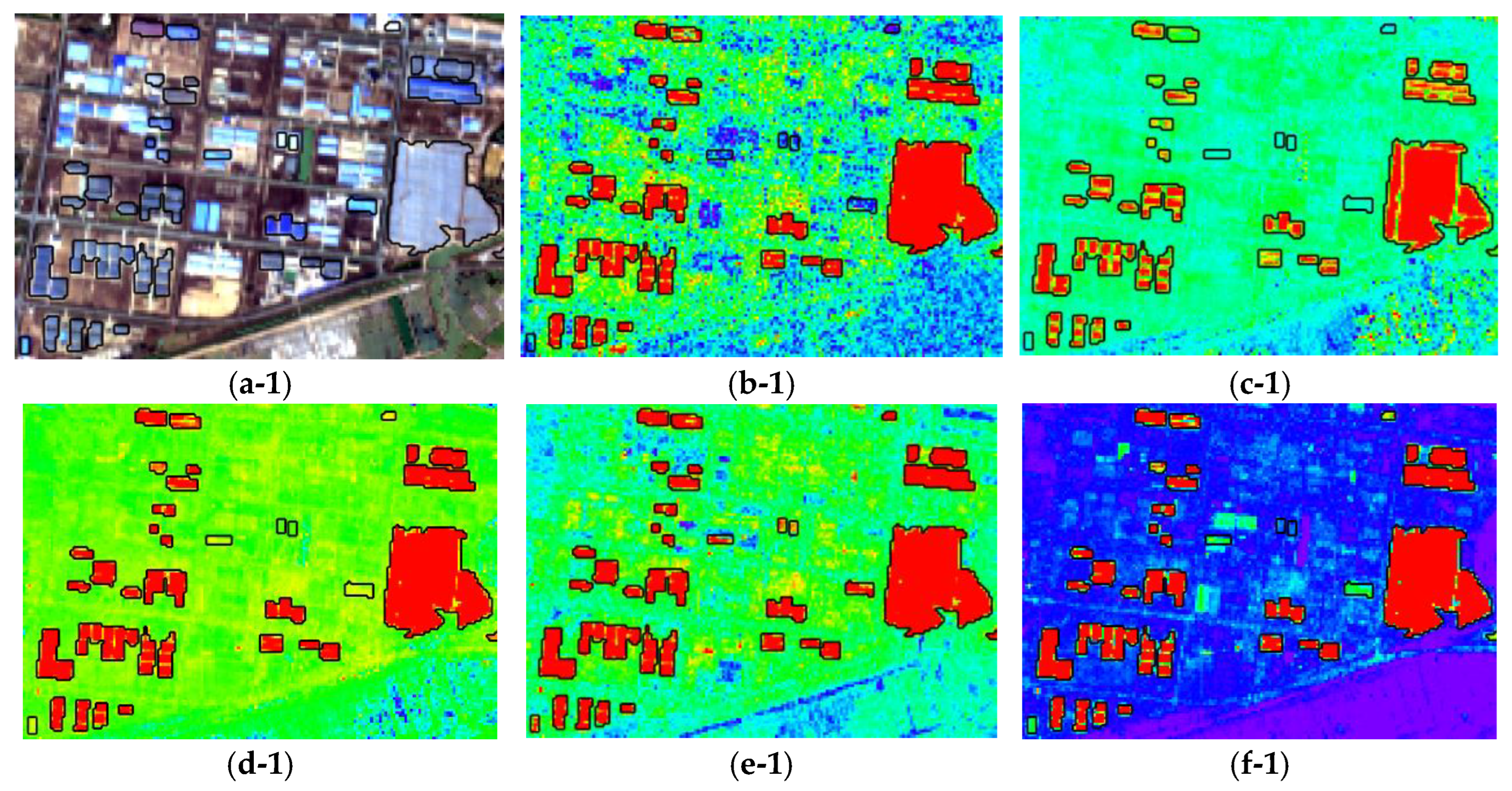
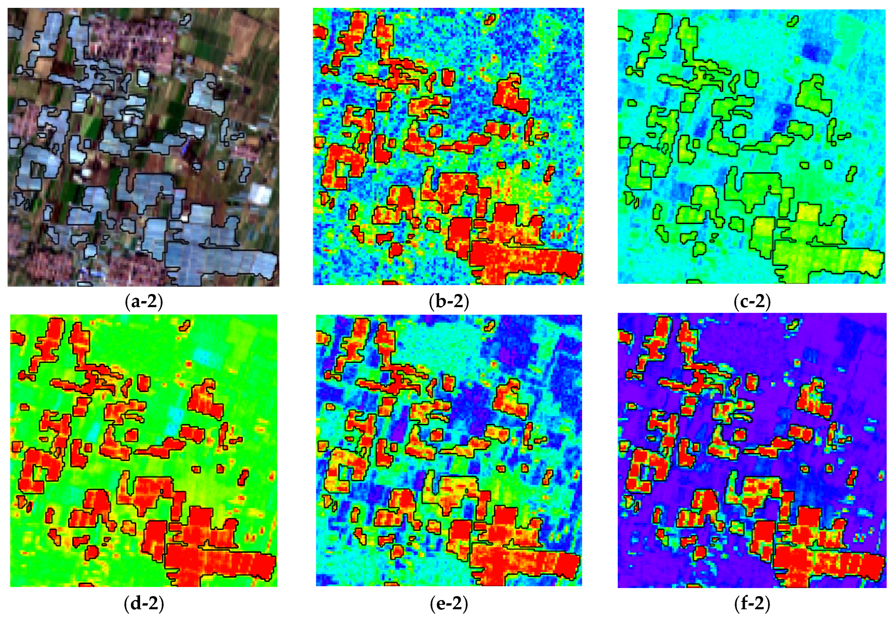
To further compare the performance of the different indices, two local image subsets were selected (Figure 10). In the industrial park (Figure 10(a-1)), nHI (Figure 10(c-1)) showed low values at plastic edges, while HI, NDPI, and cPI (Figure 10(b-1,d-1,e-1)) exhibited elevated non-plastic values (yellow-green), causing spectral confusion. In contrast, kPI (Figure 10(f-1)) consistently highlighted plastics (red) and suppressed non-plastics (blue–purple), achieving the sharpest contrast. In the village farmland (Figure 10(a-2)), nHI (Figure 10(c-2)) yielded low values for plastic mulch, hampering its discrimination from non-plastic areas. HI and cPI (Figure 10(b-1,e-1)) also showed relatively low values for some plastic areas. However, kPI (Figure 10(f-2)) consistently suppressed non-plastic areas, providing the clearest separation.

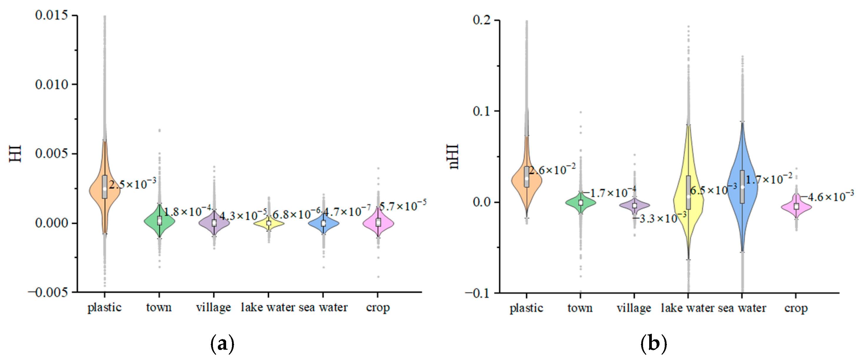
Figure 11 presents violin plots of the different indices in the Weifang area. For HI (Figure 11a) and NDPI (Figure 11c), non-plastic types exhibited numerous statistical outliers overlapping with plastic values. For nHI (Figure 11b), the value ranges for lake and sea water substantially overlapped with plastics, making differentiation difficult. For cPI (Figure 11d), the upper whiskers of urban class closely approached the interquartile range of plastics, causing spectral confusion. However, kPI (Figure 11e) revealed highly concentrated non-plastic values, well separated from plastics.

4.2.2. Separability Analysis

Table 3. Index of separability for plastics and background land covers in the Weifang area.

	Land Cover Type	HI	nHI	NDPI	cPI	kPI
TD	Town	1.78	1.88	1.97	1.92	2
	Village	1.96	1.99	2	2	2
	Lake water	2	0.35	0.93	2	2
	Sea water	1.99	0.07	1.72	2	2
	Crop	1.93	1.97	2	2	2
B-distance	Town	0.72	0.74	0.98	0.75	1.22
	Village	0.88	0.94	1.27	0.97	1.64
	Lake water	1.12	0.14	0.57	1.36	2.21
	Sea water	1	0.04	1.24	1.41	2.52
	Crop	0.83	0.88	1.33	1.06	1.89

presents the separability metrics in the Weifang area. For TD metrics, HI values fell below 1.9 in town areas, while nHI and NDPI were well below 1.7 over lake water. Both cPI and kPI showed good separability with TD values exceeding 1.9 across all background classes.

For B-distance metrics, HI, nHI, NDPI and cPI were below 1.5 and for lake water, nHI was below 0.2. kPI showed higher B-distances than other indices with a value above 1.5 for all categories except town areas for non-plastic categories, indicating better separability.

4.2.3. Plastic Mapping Results

Table 4. Accuracies for plastic mapping with different methods in the Weifang area.

Method	Threshold	F1 (%)	OA (%)	PA (%)	UA (%)
HI	0.0019	72.3	99.1	71.6	73.1
nHI	0.0732	14.2	97.7	11.0	20.0
NDPI	0.0753	78.8	99.3	81.5	76.2
iOCRF		72.4	98.7	96.2	58.0
cPI	0.0078	84.0	99.5	83.5	84.5
kPI	0.0024	85.1	99.5	84.9	85.4

Note: OA: overall accuracy; PA: plastics producer’s accuracy; UA: plastics user’s accuracy.

presents the optimal thresholds and mapping accuracies across methods in the Weifang area. While HI, NDPI, and iOCRF all had F1 scores below 80%, and nHI had an F1 score of only 14.2%, cPI achieved the highest F1-score at 84.0% with balanced UA and PA above 80%. In contrast, kPI outperformed all other methods, reaching a maximum F1-score of 85.1% and the highest UA, demonstrating the robust overall mapping performance.

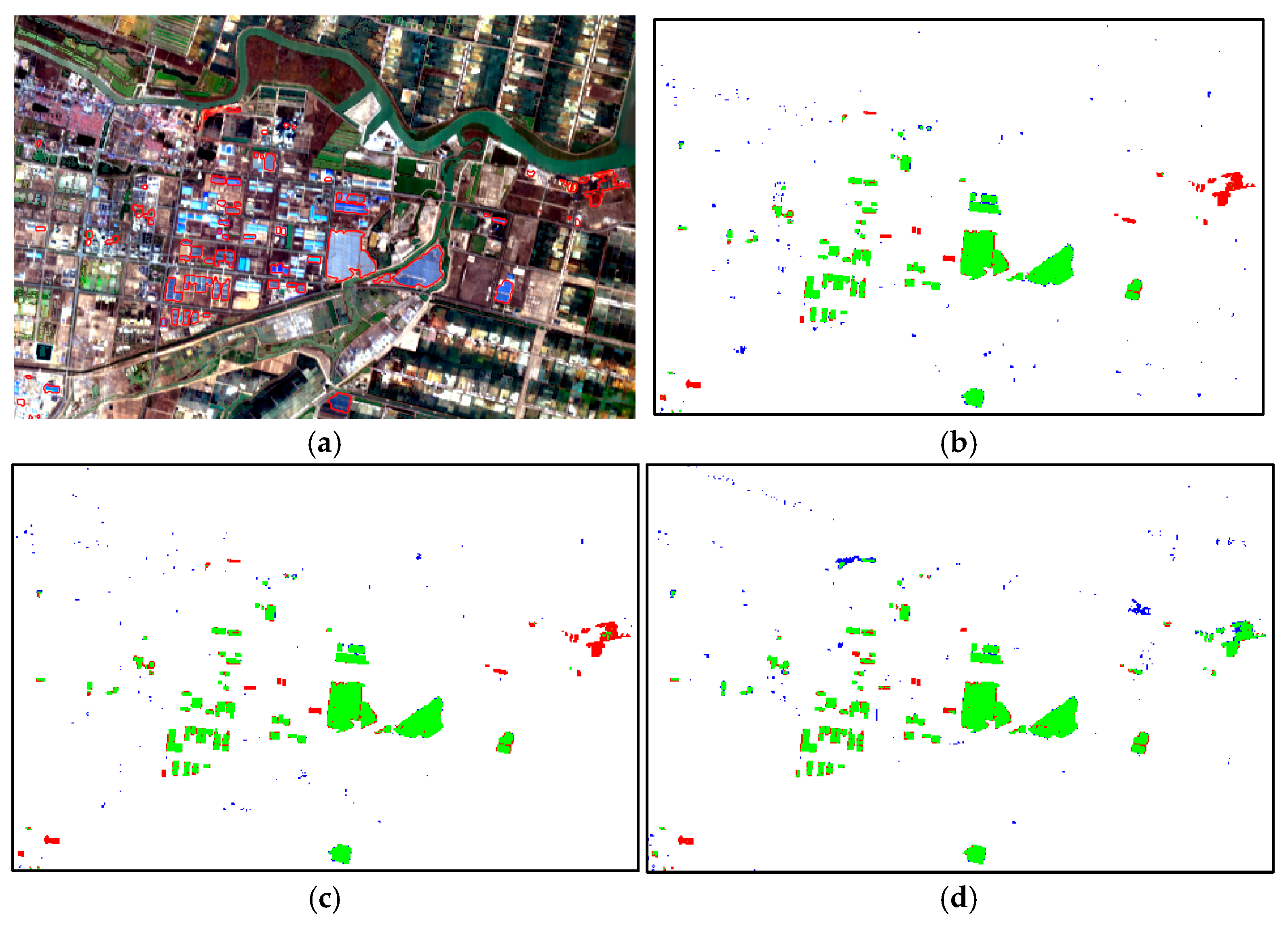
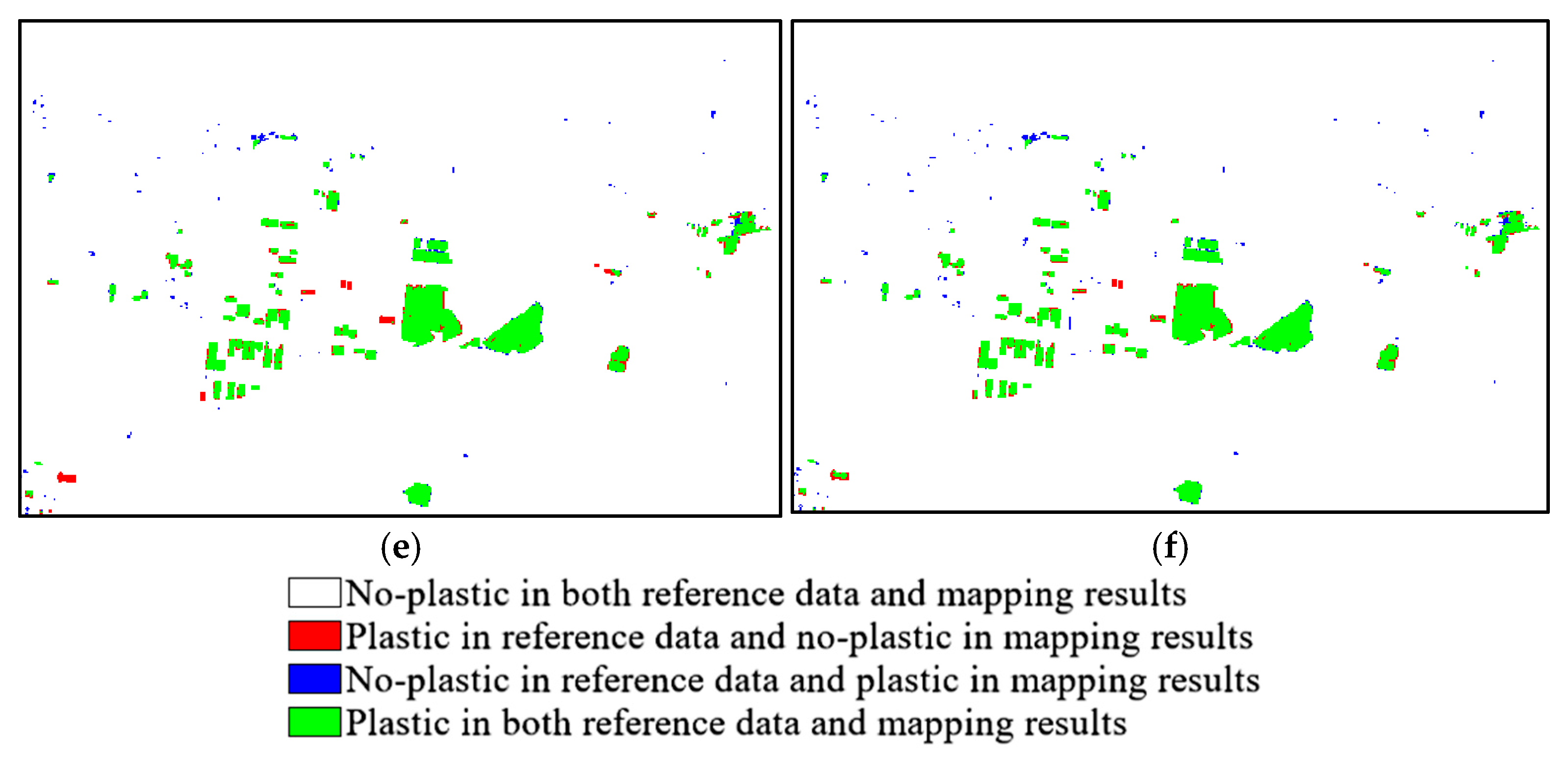
Figure 12 shows plastic mapping results in the Weifang area. As shown in Figure 12c, nHI failed to detect the plastic targets in lower-left region (marked in red) and misclassified water in the upper-right area as plastics (highlighted in blue). HI (Figure 12b) and NDPI (Figure 12d) exhibited certain underestimations (red) and also incorrectly classified certain non-plastic features as plastics (blue). Although iOCRF (Figure 12e) successfully classified most plastics, it produced extensive false positives in rural areas (shown in blue). In contrast, cPI and kPI (Figure 12f,g) showed better performance than competing methods, achieving fewer misclassified and omitted pixels.

4.3. Beijing Area

4.3.1. Qualitative Evaluation

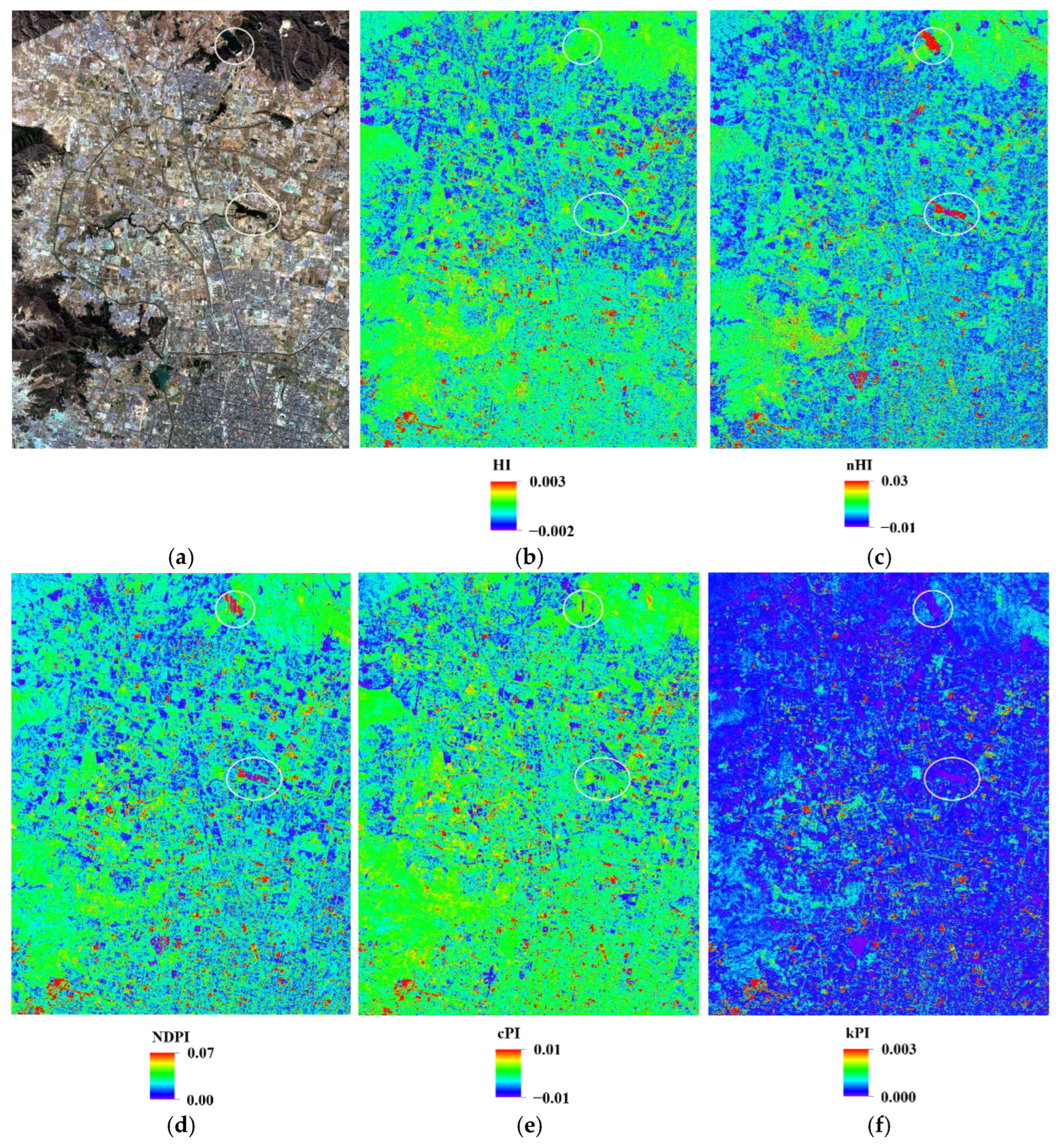
Figure 13 presents different index images for the Beijing area. In the nHI (Figure 13c) and NDPI (Figure 13d) images, the index values for the two water areas enclosed with white circles were markedly high (appeared red). In the HI (Figure 13b) and cPI (Figure 13e) images, the index values for non-plastic areas were relatively high (appeared yellow–green), which were comparable to those of plastic. In contrast, the kPI image (Figure 13f) consistently exhibited minimized index values over non-plastic areas (appeared blue–purple), and thus enabled the clearest distinction from plastic.

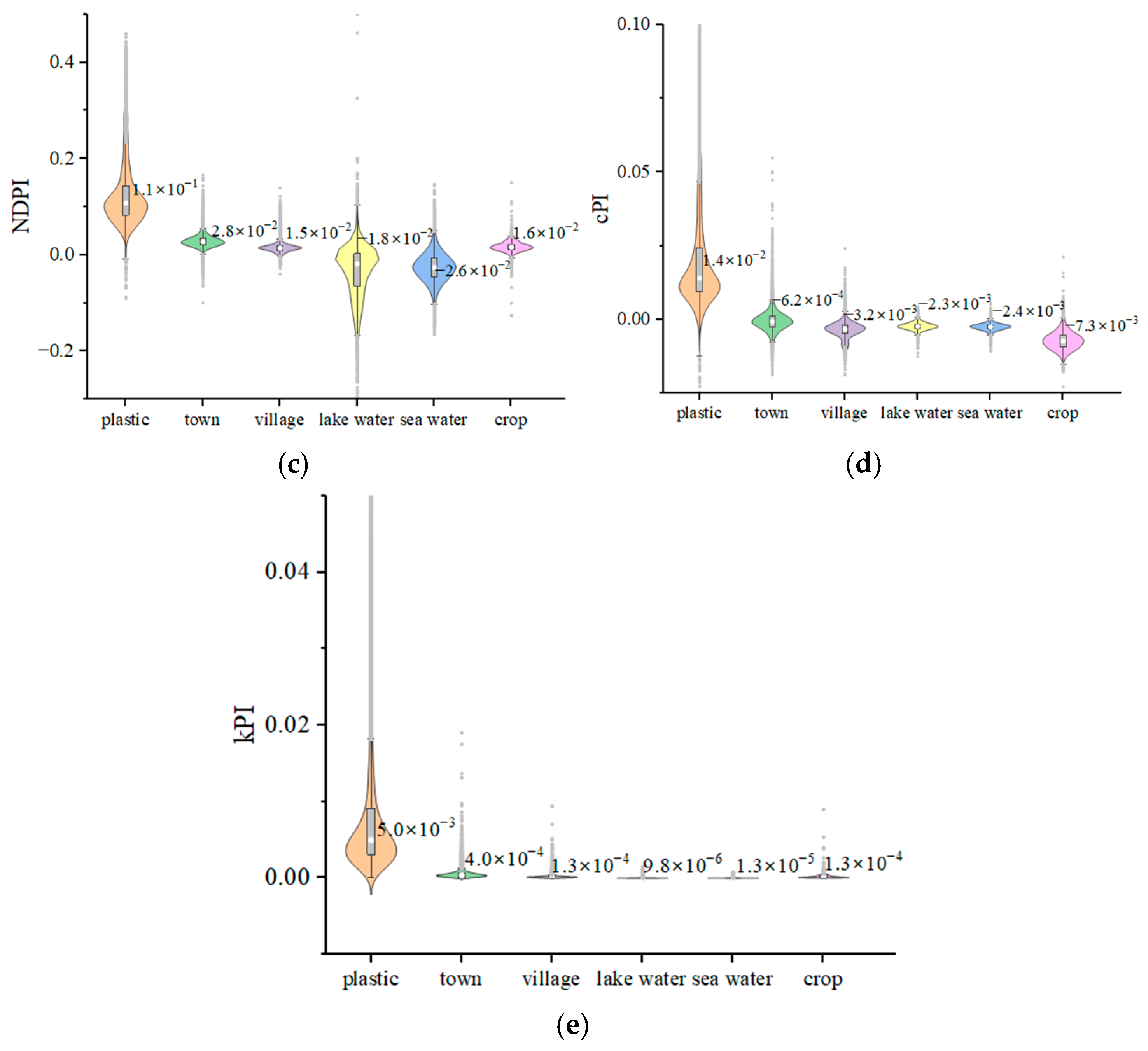
Figure 14 presents the violin plots of different spectral indices in the Beijing area. For HI (Figure 14a) and cPI (Figure 14d), non-plastic values substantially overlapped with plastic quartile ranges. For nHI (Figure 14b) and NDPI (Figure 14c), water and shadows overlapped considerably with plastic, and poor separability was observed. However, kPI (Figure 14e) values across all non-plastic classes were tightly clustered and showed minimal overlap with plastics interquartile ranges (IQRs); only certain soil and building samples exhibited marginally higher values, yielding the best overall separability.

4.3.2. Separability Analysis

Table 5. Separability metrics between plastics and background land covers in the Beijing area.

	Land Cover Type	HI	nHI	NDPI	cPI	kPI
TD	Vegetation	1.99	1.40	1.98	2	2
	Soil	1.77	1.84	1.60	1.93	2
	Buildings	1.99	1.26	1.34	1.99	2
	Road	1.99	1.74	1.97	2	2
	Shade	2	0.89	0.6	2	2
	Water	2	2	0.71	2	2
B-distance	Vegetation	0.99	0.47	0.86	1.06	1.42
	Soil	0.83	0.75	0.65	0.84	1.33
	Buildings	1.12	0.52	0.62	0.91	1.38
	Road	1.19	0.65	0.91	1.07	1.42
	Shadow	1.25	0.30	0.23	1.20	1.59
	Water	1.26	1.39	0.27	1.23	2.18

presents the separability metrics in the Beijing area. For TD metrics, most values for nHI were below 1.7. HI yielded a TD below 1.9 for soil. Both cPI and kPI achieved TD values greater than 1.9 for all backgrounds, with kPI consistently achieving 2.0, demonstrating excellent separability.

For B-distance metrics, most values for nHI and NDPI were below 1.0, while those for HI and cPI were between 0.8 and 1.3. kPI provided B-distances exceeding 1.3 for all non-plastic types and thus greater separability.

4.3.3. Plastic Mapping Results

Table 6. Accuracies for plastic mapping with different methods in the Beijing area.

Method	Threshold	F1 (%)	OA (%)	PA (%)	UA (%)
HI	0.002	82.1	94.4	74.1	91.9
nHI	0.019	65.0	86.4	72.4	59.0
NDPI	0.055	86.0	94.9	89.1	83.1
iOCRF		90.7	96.7	93.2	88.3
cPI	0.0067	91.3	97.0	88.9	93.8
kPI	0.0015	92.4	97.4	92.4	92.5

Note: OA, overall accuracy; PA, producer’s accuracy for plastics; UA, user’s accuracy for plastics.

presents plastic mapping performance of different methods in the Beijing area. Among the compared methods, nHI had the lowest F1-score at 65.0%, while HI and NDPI marginally exceeded 80%. Both cPI and iOCRF reached F1-scores over 90%. Meanwhile, kPI was better than all the other methods and reached the highest F1-score of 92.4%.

For the plastic class, PA values lower than 80% were obtained for HI, and nHI for both UA and PA. NDPI, cPI, and iOCRF obtained relatively balanced UA and PA values, all above 80%. In addition, kPI obtained UA and PA values above 90%, showing the most balanced performance and the best overall accuracy among all the methods.

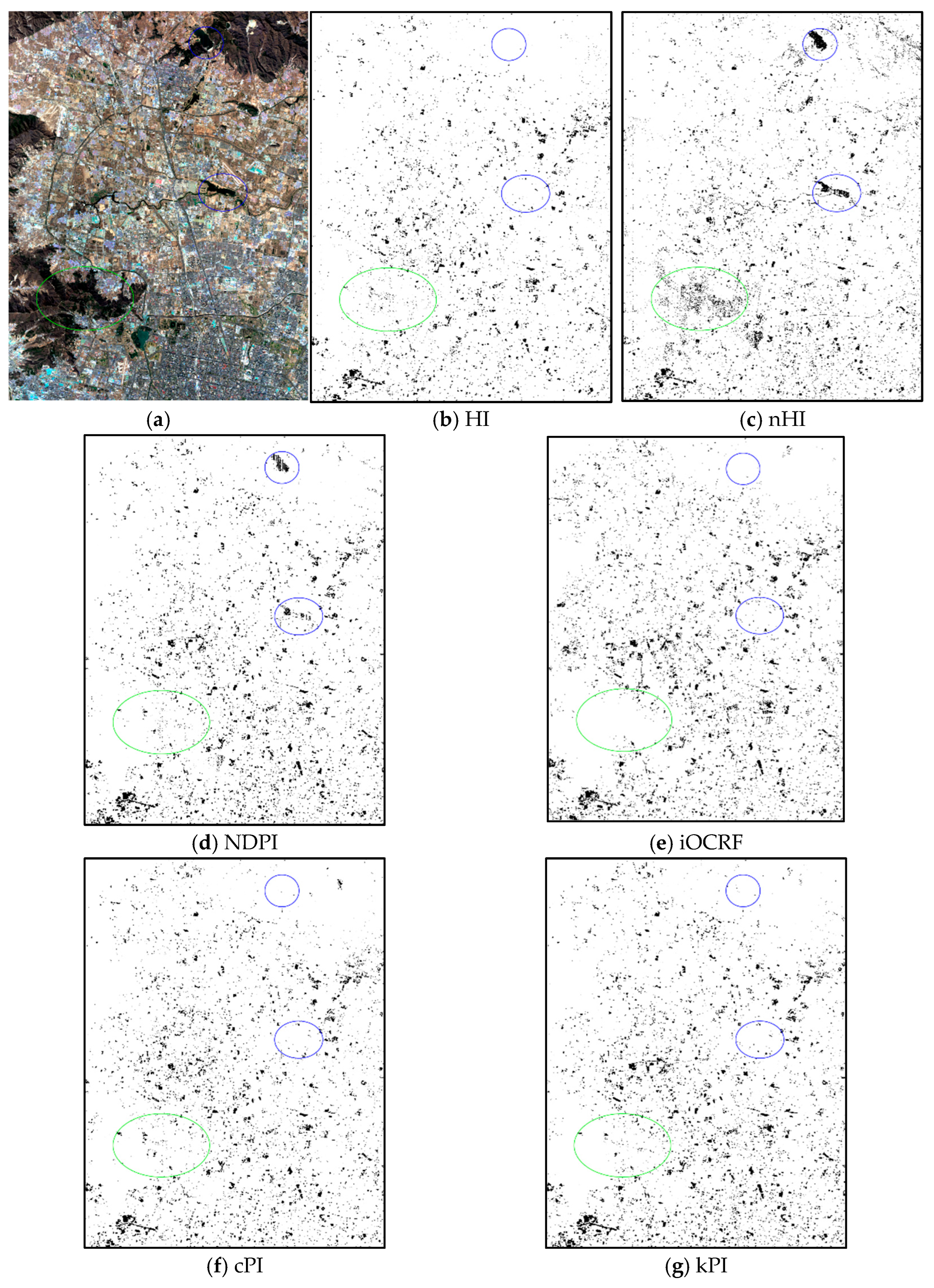
The plastic mapping results in the Beijing area are shown in Figure 15. nHI mistakenly classified vegetation (circled in green) as plastics (Figure 15c). In the water areas (circled in blue), both nHI and NDPI falsely classified water pixels as plastics (Figure 15c,d). HI, cPI, and kPI (Figure 15b,f,g) only misclassified a small amount of vegetation, whereas iOCRF (Figure 15e) demonstrated the lowest rate of misclassifying non-plastic features into plastics.

Comparative experiments have demonstrated that kPI outperforms existing spectral indices in terms of qualitative evaluation, separability analysis, and plastic mapping accuracy. Across different sensors and research scenarios, kPI effectively enhances plastic targets while suppressing background objects, achieving the highest F1-score.

5. Discussion

5.1. Sensitivity Analysis of the Weighting Factor in nPI

A sensitivity analysis was conducted on the weighting factor of the first absorption feature in nPI construction (Equation (1)) to verify the stability of this empirical parameter selection. A typical local area was selected from each of the three study areas (Figure 16), and the weighting factor of the first absorption feature in nPI (Equation (1)) was adjusted from 1 to 3 with a step of 0.5. Taking the nPI result with a weighting factor of 2 as the baseline, the Pearson correlation coefficient (Pearson r), root mean square error (RMSE) and bias were used to quantify the discrepancies in the index results under different weights.

The quantitative statistical results are presented in

Table 7. Statistical results of nPI discrepancies relative to the baseline with a weighting factor of 2.

	Weighting Factor	Pearson r	RMSE	Bias
Guangzhou	1	0.9835	0.0125	−0.0056
	1.5	0.9975	0.0049	−0.0022
	2.5	0.9988	0.0035	0.0015
	3	0.9963	0.0061	0.0027
Weifang	1	0.9976	0.0132	0.0118
	1.5	0.9996	0.0051	0.0046
	2.5	0.9997	0.0036	−0.0032
	3	0.9991	0.0062	−0.0055
Beijing	1	0.9934	0.0122	0.0112
	1.5	0.9988	0.0048	0.0044
	2.5	0.9993	0.0034	−0.0031
	3	0.9976	0.0059	−0.0054

. Compared with the baseline results obtained with a weighting factor of 2, the Pearson correlation coefficients under all comparative weighting values are higher than 0.98, the RMSE values are all less than 0.013, and the absolute values of bias are all less than 0.012, indicating that the discrepancies are very small in absolute terms.

It can also be observed that the discrepancies at weighting factors of 1.5 and 2.5 are slightly smaller than those at 1 and 3, which is consistent with the expectation that the index behaves most stably in the vicinity of the selected baseline value. Nevertheless, even at the extreme weights of 1 and 3, the Pearson r remains above 0.98 and the RMSE remains below 0.013. This indicates that, within a reasonable parameter range, the weight of the first absorption feature has only a limited influence on the nPI (Equation (1)), and the weighting factor selected in this study (2) is robust and physically justifiable.

5.2. Effect of the Kernel Width Parameter σ on Mapping Accuracy Using kPI

In kPI, the kernel width σ serves as a core parameter controlling the samples influence range in the feature space. An excessively small σ leads to local overfitting, whereas an overly large σ reduces class separability [27,28].

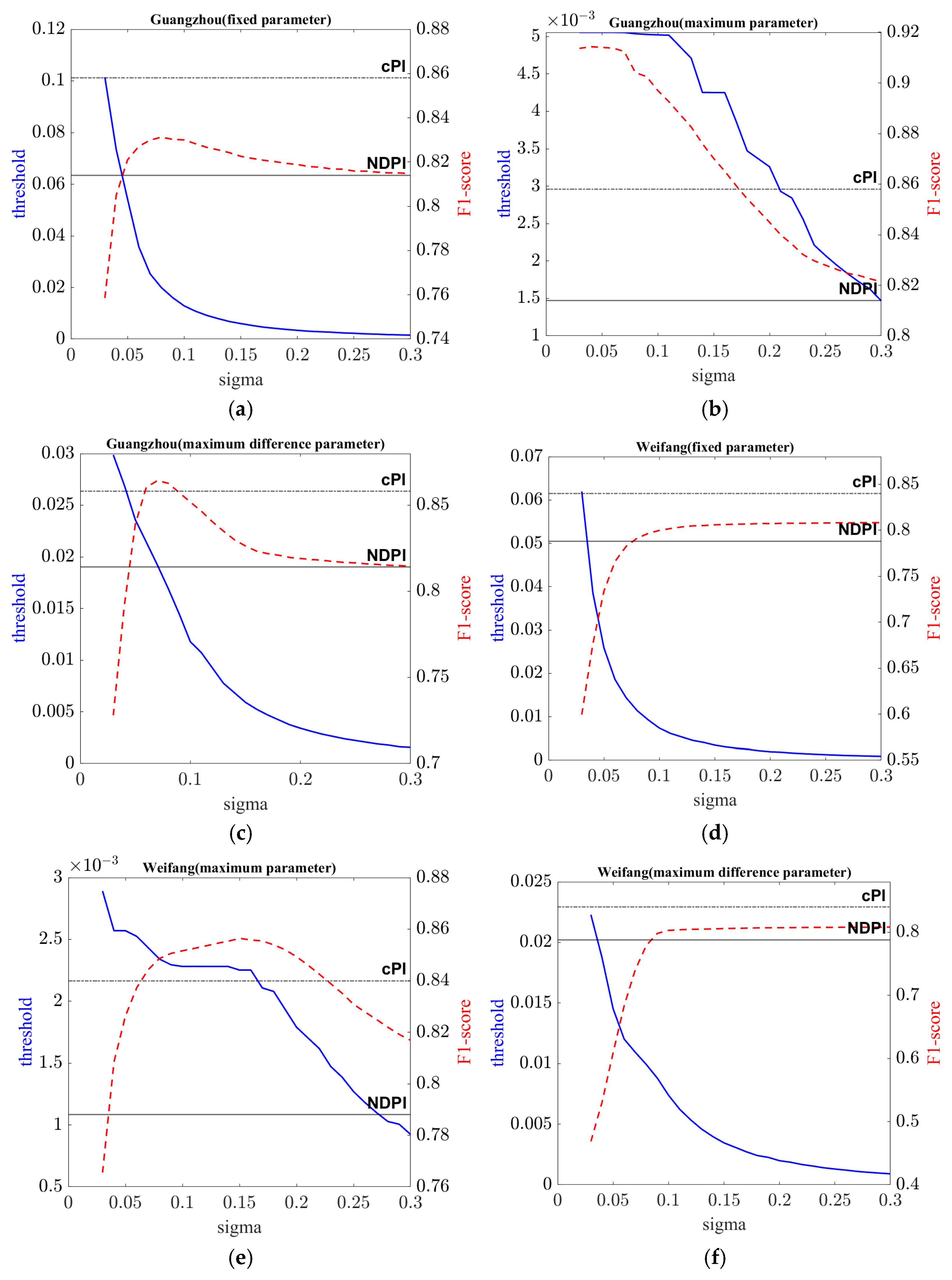
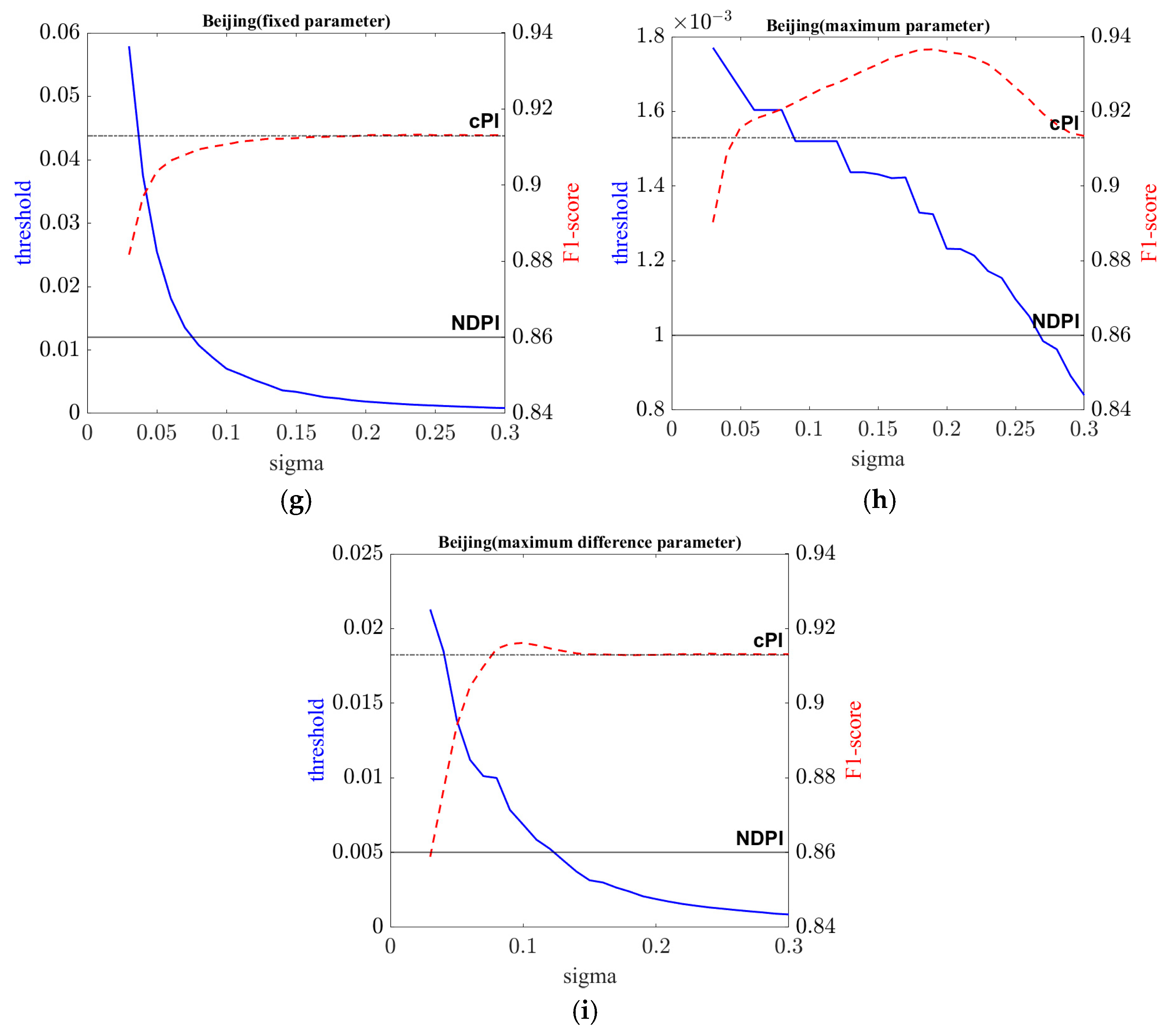
In this study, the σ parameter was determined using three different approaches: the fixed, the maximum, and the maximum difference parameter methods were evaluated across constant n values ranging from 0.03 to 0.3 (step = 0.01).

Figure 17 presents the optimal thresholds and corresponding mapping accuracies across the three study areas. As shown in Figure 17, the maximum method consistently achieved higher F1-scores than other methods and indices. In the Guangzhou area, the highest accuracy was achieved when n ≈ 0.07 (Figure 17b), while the optimal n values for the Beijing and Weifang areas were 0.18 and 0.15 (Figure 17e,h), respectively. In contrast, the fixed parameter and the maximum difference method were roughly comparable to cPI, with the optimal n values of approximately 0.07 in Guangzhou (Figure 17a,c) and 0.1 in Weifang and Beijing (Figure 17d,f,g,i).

The noticeable discrepancy in the optimal n value across study areas within the maximum method is closely related to background land covers (including low-reflectance targets), sensor type and spatial resolution.

On the one hand, background land covers are a major driver for optimal n selection. In the UAV hyperspectral scene in Guangzhou study area, the background is relatively simple, primarily composed of impervious surfaces (e.g., concrete and brick pavements), vegetation, and bare soil, with virtually no shadows or open water bodies. Because the mean reflectance of these background materials remains at a moderate-to-high level, a smaller n value (0.07) is sufficient to avoid numerical instability while providing stronger dynamic contrast stretching. In contrast, the GF-5 hyperspectral scenes in Weifang and Beijing encompass complex background land-cover categories, including low-reflectance targets (such as seawater, aquaculture ponds, lakes, and building shadows). If n is set too small, the σ values of such targets approach zero alongside their mean reflectance, inducing severe noise. Therefore, in these complex terrestrial scenes, a larger n value is indispensable to suppress background fluctuations, which aligns better with practical and complex remote sensing application demands.

On the other hand, the optimal n value is also closely related to the sensor type and spatial resolution. The Guangzhou dataset was acquired by a UAV-borne hyperspectral sensor with a very high spatial resolution, where individual pixels are relatively pure and mixed-pixel effects are weak. Consequently, the background reflectance statistics are more stable, and a smaller n value is sufficient. In contrast, the GF-5 scenes were acquired by a satellite hyperspectral sensor with a coarser spatial resolution, a single pixel often covers multiple land-cover types, resulting in more pronounced mixed-pixel effects and more heterogeneous background reflectance. Moreover, differences in spectral response functions, band configurations, signal-to-noise ratios, and radiometric calibration between the UAV and GF-5 sensors further alter the measured reflectance statistics and noise levels. These sensor- and resolution-related factors jointly cause the background reflectance within GF-5 pixels to fluctuate more markedly, thereby requiring a larger n value to suppress background noise and maintain stable enhancement performance.

The advantage of the maximum method stems from two factors. First, the pixel-wise adaptive parameter considers the spectral variation between different land cover types, alleviating the limited generalizability of a fixed parameter. Second, imposing n as a lower bound suppresses background noise over low-reflectance surfaces (e.g., shadows and water bodies), where adaptive values become unstable. Although this method yields relatively low optimal thresholds that narrow the effective value range and reduce visual contrast, constraining n within 0.1–0.15 consistently achieves high mapping accuracy across all study areas.

5.3. Effect of Different Band Combinations in kPI on Plastic Mapping

To further validate the effectiveness of kPI and investigate the impact of different band combinations on mapping performance, this study employed a controlled-variable approach to design four different band combinations, formulated as

$$nP{I}_1={\displaystyle \frac{R_A-R_B}{R_A+R_B}}$$

(21)

$$nP{I}_2={\displaystyle \frac{R_A+R_C-2R_B}{R_A+R_C+2R_B}}$$

(22)

$$nP{I}_3={\displaystyle \frac{R_D-R_E}{R_D+R_E}}$$

(23)

$$nP{I}_4={\displaystyle \frac{R_A-R_B+R_D-R_E}{R_A+R_B+R_D+R_E}}$$

(24)

where the definitions of bands A–E are identical to those in Section 2.2, ${nPI}_1$, ${nPI}_2$, and ${nPI}_3$ are based on single absorption features, ${nPI}_4$ and nHI are based on two absorption features.

According to the derivation method in this study, the four kernel-based counterparts corresponding to nPI₁–nPI₄ are as follows:

$$kP{I}_1={\displaystyle \frac{1-k(R_A,R_B)}{1+k(R_A,R_B)}}$$

(25)

$$kP{I}_2={\displaystyle \frac{3+k(R_A,R_C)-2k(R_A,R_B)-2k(R_B,R_C)}{3+k(R_A,R_C)+2k(R_A,R_B)+2k(R_B,R_C)}}$$

(26)

$$kP{I}_3={\displaystyle \frac{1-k(R_D,R_E)}{1+k(R_D,R_E)}}$$

(27)

$$kP{I}_4={\displaystyle \frac{\begin{array}{l}2+k(R_A,R_D)+k(R_B,R_E)-k(R_A,R_B)\\ -k(R_A,R_E)-k(R_B,R_D)-k(R_D,R_E)\end{array}}{\begin{array}{l}2+k(R_A,R_D)+k(R_B,R_E)+k(R_A,R_B)\\ +k(R_A,R_E)+k(R_B,R_D)+k(R_D,R_E)\end{array}}}$$

(28)

Table 8. Plastic mapping accuracy across different combinations in kPI index formats in each study area.

Index	Guangzhou		Weifang		Beijing
	Threshold	F1 (%)	Threshold	F1 (%)	Threshold	F1 (%)
${kPI}_1$	0.022	89.3	0.0015	78.2	0.0004	75.0
${kPI}_2$	0.0062	89.4	0.0006	68.6	0.0002	83.5
${kPI}_3$	0.030	43.1	0.017	81.8	0.012	89.2
${kPI}_4$	0.011	88.7	0.0057	84.4	0.0031	91.7
$kPI$	0.0055	89.6	0.0024	85.1	0.0015	92.4

shows mapping accuracies for different kPI variants. ${kPI}_1$, ${kPI}_2$, and ${kPI}_3$ exhibited considerable variation across the three study areas, strongly correlated with the absorption depth of the corresponding absorption feature. In contrast, ${kPI}_4$ and $kPI$ achieved F1 scores above 84% in all three areas, with kPI consistently highest. Compared to ${kPI}_4$, kPI incorporates the right shoulder C of the first absorption feature. However, the inclusion of the shoulder C led to an overall decrease in the optimal threshold, which consequently resulted in consistently lower index values and reduced visual interpretability of the resulting index maps.

Figure 18 presents the plastic mapping results for the kPI formulations across the Weifang area. The ${kPI}_1$ and ${kPI}_2$ were found to leave a considerable proportion of plastic targets undetected on the right side of the area (Figure 18b,c), whereas ${kPI}_3$ falsely classified extensive non-plastic features as plastics (Figure 18d). In contrast, both ${kPI}_4$ and kPI effectively eliminated both the omission of true plastics and the misclassification of background materials, yielding markedly cleaner mapping layouts (Figure 18e,f).

From the above observations, kPI based on two absorption features maintains consistently high accuracy across all study areas. Furthermore, by incorporating the complete three-band configuration of the first absorption feature, the mapping performance was further optimized.

5.4. Advantages of kPI

kPI offers three main advantages over existing methods.

First, kPI jointly uses two diagnostic absorption features of plastics (1600–1800 nm and 2000–2400 nm) to account for spectral variability among different plastic types. Existing HI and nHI rely only on the 1730 nm feature and fail to accommodate aromatic plastics, due to the shift in the absorption peak toward shorter wavelengths and reduced absorption magnitude. Although NDPI combines two absorption features, it is derived from WorldView-3 imagery, which cannot accurately match the actual absorption locations. By contrast, cPI and kPI use the two diagnostic absorption features defined by five SWIR bands, enhancing robustness for diverse plastic types.

Second, existing plastic spectral indices (including cPI) use linear band combinations (e.g., differences, ratios, and normalized combinations). However, these formulations often fail to effectively separate plastics from non-plastic materials, resulting in limited discriminability. In contrast, kPI employs a Gaussian RBF kernel to map the two absorption features into a higher-order nonlinear feature space. This nonlinear transformation enhances plastic signals while suppressing responses from other land cover types, effectively increasing spectral contrast between plastics and non-plastics. Consequently, kPI achieves higher spectral separability and mapping accuracy than the comparative methods.

Third, compared with the iOCRF classification method, kPI achieves higher and more stable accuracy across the three study areas. This advantage was consistent under the specific conditions of this study. It should be noted, however, that the two approaches have different objectives and operational requirements: kPI is a deterministic spectral transformation followed by thresholding, whereas iOCRF is a learned one-class classifier that does not require a predefined threshold. The higher accuracy of kPI may partly reflect the fact that iOCRF randomly extracts non-target (i.e., non-plastic) samples from the unlabeled background, which may not adequately represent the diverse spectral features of complex scenes, particularly when the number of labeled target samples is limited. In addition, the richer spatial details in UAV data may introduce greater within-class spectral variability, making the randomly extracted non-target samples more likely to be spectrally confounded with the target class and thus degrading iOCRF’s classification performance. These factors jointly result in relatively low accuracy of iOCRF across all study areas. Given these limitations, the performance of other classification methods for plastic mapping warrants further investigation in future work.

5.5. Limitations and Future Research

Although the proposed kPI demonstrates superior plastic mapping capabilities across both UAV and satellite scales, several limitations warrant in-depth discussion for practical remote sensing applications in complex terrestrial environments:

First, the impact of mixed pixels in complex urban environments presents a notable challenge. The GF-5 reference samples used for evaluation in this study were pure or nearly pure plastic pixels, selected from large, homogeneous plastic surfaces (e.g., plastic greenhouses and artificial turf), and were nearly entirely or predominantly covered by plastics, so the accuracy assessment is not affected by sub-pixel mixing. However, plastic targets in urban built-up areas (such as small shed roofs, scattered domestic waste, and temporary protective covers) are typically small and fragmented. When observed using hyperspectral imagery at 30 m spatial resolution, plastic targets rarely occupy an entire pixel and predominantly exist as mixed pixels. Under linear mixing, the spectral contributions of surrounding background materials (e.g., concrete pavements, asphalt, and bare soil) attenuate the diagnostic absorption features across the shortwave-infrared (SWIR) bands, and the kPI response decreases with decreasing plastic fractional cover. Below a certain fractional cover, the absorption feature becomes indistinguishable from noise, potentially elevating omission risks for low-abundance plastic targets.

Second, reference sample configurations and threshold calibration impose certain constraints in the Guangzhou area with the UAV hyperspectral data, where plastic targets were deployed as individual sheets. Although diverse polymer types were represented, the total number of plastic targets was relatively limited. Consequently, during random sample partitioning, the distinction between the threshold-optimization subset and the test subset within plastic targets remains small, with potential local spatial autocorrelation. In addition, the kPI relies on threshold-based decision rules, and the optimal threshold may vary with sensor configuration, atmospheric conditions, and surface background, which limits direct transferability across scenes.

Third, sensor configurations and atmospheric correction introduce certain uncertainties. Specifically, discrepancies among hyperspectral sensors in spectral resolution, band-center locations, and signal-to-noise ratios (SNR) lead to slight variations in the captured plastic absorption profiles. In addition, the quality of atmospheric correction also affects the stability of the proposed kPI.

Fourth, the impact of spatial autocorrelation on random sample partitioning differs between the two observation scales. For the GF-5 hyperspectral data (30 m spatial resolution), the plastic targets used as reference samples are predominantly small and isolated, or occur as mixed pixels; a single physical object therefore rarely covers multiple pure plastic pixels, and inter-pixel correlation is weak. In contrast, for the UAV hyperspectral data in the Guangzhou area, plastic targets were deployed in two sections: 24 uniform plastic plates in the right section and clusters of plastic bags and bottles of varying sizes in the left section. The two sections differ in spatial consistency: the plates are highly uniform, leading to relatively strong local spatial autocorrelation, whereas the bag/bottle clusters are more heterogeneous, leading to weaker autocorrelation. Because the total number of independent spatial clusters is limited, random sample partitioning cannot fully separate the threshold-optimization subset from the test subset within individual objects, and local spatial autocorrelation may remain. The reported accuracy for the UAV data should therefore be regarded as an upper-bound estimate. Future work should collect a larger number of independent plastic objects and adopt object-based validation, in which entire objects or spatial regions are withheld from threshold optimization and used exclusively for testing.

Fifth, spectral variability within the same polymer type and the effects of weathering and ageing remains to be addressed. Plastics of the same polymer type can exhibit different spectral signatures due to differences in additives, fillers, surface roughness, and manufacturing processes. Weathering and ageing further alter surface chemistry and can weaken the diagnostic absorption features, potentially reducing kPI performance for aged plastics in real environments. The plastics used in this study were virgin samples, so these effects warrant further investigation.

Future research should integrate spectral unmixing to further assess the capability of plastic identification under mixed pixel conditions, and explore adaptive unsupervised thresholding algorithms to improve cross-scene applicability. Colour and thickness can modulate reflectance magnitude and absorption depth, and their effects merit evaluation in future work. Beyond these technical factors, environmental and seasonal variations also deserve consideration. The current datasets were acquired during spring and autumn; hence, the performance of the proposed index under different seasons requires further investigation. Furthermore, complex urban environments may introduce additional spectral interference from artificial surfaces and shadowing, which could affect the robustness of kPI and thus merit dedicated assessment. Moreover, further investigations are necessary to evaluate the performance of the kPI on hyperspectral data such as PRISMA and EnMAP, as well as its potential for mapping plastics in other environments.

6. Conclusions

This study proposes a novel kernel-based hyperspectral index, kPI, for highlighting and mapping plastics in urban built-up areas. kPI utilizes two diagnostic SWIR absorption features with the Gaussian RBF kernel to enable nonlinear feature mapping. This nonlinear mapping is particularly critical for enhancing the spectral contrast between plastics and other land cover types while accommodating spectral variability among different plastic types. Experimental results demonstrate that kPI consistently exhibits better separability between plastics and other land cover types, and achieves higher mapping accuracy compared to comparative indices and the iOCRF classification method. The distinctive advantage of kPI lies in its strong sensitivity to plastics and robust suppression to other land cover types. kPI provides an effective and robust variable for operational plastic mapping in urban environments.

References

1. Geyer, R. Chapter 2—Production, use, and fate of synthetic polymers. In Plastic Waste and Recycling; Geyer, R., Ed.; Academic Press: London, UK, 2020; pp. 13–32. [Google Scholar]
2. Letcher, T.M. Chapter 1—Introduction to plastic waste and recycling. In Plastic Waste and Recycling; Letcher, T.M., Ed.; Academic Press: London, UK, 2020; pp. 3–12. [Google Scholar]
3. Paterson, H. Plastic habits—An overview for the collection ‘Plastics and Sustainable Earth’. Sustain. Earth 2019, 2, 10. [Google Scholar] [CrossRef] [Scilit]
4. Veettil, B.K.; Doan Van, D.; Quang, N.X.; Hoai, P.N. Remote sensing of plastic-covered greenhouses and plastic-mulched farmlands: Current trends and future perspectives. Land Degrad. Dev. 2022, 34, 591–609. [Google Scholar] [CrossRef] [Scilit]
5. Zhang, Y.; Wang, X.; Shan, J.; Zhao, J.; Zhang, W.; Liu, L.; Wu, F. Hyperspectral Imaging Based Method for Rapid Detection of Microplastics in the Intestinal Tracts of Fish. Environ. Sci. Technol. 2019, 53, 5151–5158. [Google Scholar] [CrossRef] [Scilit] [PubMed]
6. Zheng, J.; Suh, S. Strategies to reduce the global carbon footprint of plastics. Nat. Clim. Change 2019, 9, 374–378. [Google Scholar] [CrossRef] [Scilit]
7. Ford, H.V.; Jones, N.H.; Davies, A.J.; Godley, B.J.; Jambeck, J.R.; Napper, I.E.; Suckling, C.C.; Williams, G.J.; Woodall, L.C.; Koldewey, H.J. The fundamental links between climate change and marine plastic pollution. Sci. Total Environ. 2022, 806, 150392. [Google Scholar] [CrossRef] [Scilit] [PubMed]
8. Hurley, R.; Horton, A.; Lusher, A.; Nizzetto, L. Chapter 7—Plastic waste in the terrestrial environment. In Plastic Waste and Recycling; Hurley, R., Horton, A., Lusher, A., Nizzetto, L., Eds.; Academic Press: London, UK, 2020; pp. 163–193. [Google Scholar]
9. Horton, A.A.; Walton, A.; Spurgeon, D.J.; Lahive, E.; Svendsen, C. Microplastics in freshwater and terrestrial environments: Evaluating the current understanding to identify the knowledge gaps and future research priorities. Sci. Total Environ. 2017, 586, 127–141. [Google Scholar] [CrossRef] [Scilit] [PubMed]
10. Barnes, D.K.A.; Galgani, F.; Thompson, R.C.; Barlaz, M.A. Accumulation and fragmentation of plastic debris in global environments. Philos. Trans. R. Soc. B 2009, 364, 1985–1998. [Google Scholar] [CrossRef] [Scilit] [PubMed]
11. Brglez, K.; Čuček, L.; Krajnc, D.; Kovačič Lukman, R. Assessing the environmental impact of plastic flows in urban areas: A life cycle assessment and scenario analysis study. J. Clean. Prod. 2024, 449, 141761. [Google Scholar] [CrossRef] [Scilit]
12. Maharjan, N.; Miyazaki, H.; Pati, B.M.; Dailey, M.N.; Shrestha, S.; Nakamura, T. Detection of River Plastic Using UAV Sensor Data and Deep Learning. Remote Sens. 2022, 14, 3049. [Google Scholar] [CrossRef] [Scilit]
13. Liu, X.; Xiao, B.; Jiao, J.; Hong, R.; Li, Y.; Liu, P. Remote sensing detection and mapping of plastic greenhouses based on YOLOX+: A case study in Weifang, China. Comput. Electron. Agric. 2024, 218, 108702. [Google Scholar] [CrossRef] [Scilit]
14. Balsi, M.; Moroni, M.; Bouchelaghem, S. Plastic Litter Detection in the Environment Using Hyperspectral Aerial Remote Sensing and Machine Learning. Remote Sens. 2025, 17, 938. [Google Scholar] [CrossRef] [Scilit]
15. Kozloski, R.; Cowger, W.; Arienzo, M.M. Moving toward automated µFTIR spectra matching for microplastic identification: Addressing false identifications and improving accuracy. Microplast. Nanoplast. 2024, 4, 27. [Google Scholar] [CrossRef] [Scilit]
16. Siddiqui, A.; Chauhan, P.; Kumar, V.; Jain, G.; Deshmukh, A.; Kumar, P. Characterization of urban materials in AVIRIS-NG data using a mixture tuned matched filtering (MTMF) approach. Geocarto Int. 2022, 37, 332–347. [Google Scholar] [CrossRef] [Scilit]
17. Manohar Kumar, C.V.S.S.; Salini, M.S.; Nidamanuri, R.R. Abundance of Plastic-Litter in Hyperspectral Imagery Using Spectral Unmixing in Coastal Environment. In Proceedings of the IGARSS 2023—2023 IEEE International Geoscience and Remote Sensing Symposium; IEEE: New York, NY, USA, 2023; pp. 6029–6032. [Google Scholar]
18. Castagna, A.; Dierssen, H.M.; Devriese, L.I.; Everaert, G.; Knaeps, E.; Sterckx, S. Evaluation of historic and new detection algorithms for different types of plastics over land and water from hyperspectral data and imagery. Remote Sens. Environ. 2023, 298, 113834. [Google Scholar] [CrossRef] [Scilit]
19. Aguilar, M.A.; Jiménez-Lao, R.; Aguilar, F.J. Evaluation of Object-Based Greenhouse Mapping Using WorldView-3 VNIR and SWIR Data: A Case Study from Almería (Spain). Remote Sens. 2021, 13, 2133. [Google Scholar] [CrossRef] [Scilit]
20. Guo, X.; Li, P. Mapping plastic materials in an urban area: Development of the normalized difference plastic index using WorldView-3 superspectral data. ISPRS J. Photogramm. Remote Sens. 2020, 169, 214–226. [Google Scholar] [CrossRef] [Scilit]
21. Schmidt, T.; Kuester, T.; Smith, T.; Bochow, M. Potential of Optical Spaceborne Sensors for the Differentiation of Plastics in the Environment. Remote Sens. 2023, 15, 2020. [Google Scholar] [CrossRef] [Scilit]
22. Kühn, F.; Oppermann, K.; Hörig, B. Hydrocarbon Index—An algorithm for hyperspectral detection of hydrocarbons. Int. J. Remote Sens. 2004, 25, 2467–2473. [Google Scholar] [CrossRef] [Scilit]
23. Ji, C.; Bachmann, M.; Esch, T.; Feilhauer, H.; Heiden, U.; Heldens, W.; Hueni, A.; Lakes, T.; Metz-Marconcini, A.; Schroedter-Homscheidt, M. Solar photovoltaic module detection using laboratory and airborne imaging spectroscopy data. Remote Sens. Environ. 2021, 266, 112692. [Google Scholar] [CrossRef] [Scilit] [PubMed]
24. Zhou, S.; Kuester, T.; Bochow, M.; Bohn, N.; Brell, M.; Kaufmann, H. A knowledge-based, validated classifier for the identification of aliphatic and aromatic plastics by WorldView-3 satellite data. Remote Sens. Environ. 2021, 264, 112598. [Google Scholar] [CrossRef] [Scilit]
25. Ma, L.; Peng, Y.; Pei, Y.; Zeng, J.; Shen, H.; Cao, J.; Qiao, Y.; Wu, Z. Systematic discovery about NIR spectral assignment from chemical structural property to natural chemical compounds. Sci. Rep. 2019, 9, 9503. [Google Scholar] [CrossRef] [Scilit] [PubMed]
26. Camps-Valls, G.; Campos-Taberner, M.; Moreno-Martínez, Á.; Walther, S.; Duveiller, G.; Cescatti, A.; Mahecha, M.D.; Muñoz-Marí, J.; García-Haro, F.J.; Guanter, L.; et al. A unified vegetation index for quantifying the terrestrial biosphere. Sci. Adv. 2021, 7, eabc7447. [Google Scholar] [CrossRef] [Scilit] [PubMed]
27. Wang, Q.; Moreno-Martínez, Á.; Muñoz-Marí, J.; Campos-Taberner, M.; Camps-Valls, G. Estimation of vegetation traits with kernel NDVI. ISPRS J. Photogramm. Remote Sens. 2023, 195, 408–417. [Google Scholar] [CrossRef] [Scilit]
28. Xu, H.; Sun, H.; Xu, Z.; Wang, Y.; Zhang, T.; Wu, D.; Gao, J. kNDMI: A kernel normalized difference moisture index for remote sensing of soil and vegetation moisture. Remote Sens. Environ. 2025, 319, 114621. [Google Scholar] [CrossRef] [Scilit]
29. Camps-Valls, G.; Gomez-Chova, L.; Munoz-Mari, J.; Vila-Frances, J.; Calpe-Maravilla, J. Composite kernels for hyperspectral image classification. IEEE Geosci. Remote Sens. Lett. 2006, 3, 93–97. [Google Scholar] [CrossRef] [Scilit]
30. Hase, N.; Doktor, D.; Rebmann, C.; Dechant, B.; Mollenhauer, H.; Cuntz, M. Identifying the main drivers of the seasonal decline of near-infrared reflectance of a temperate deciduous forest. Agric. For. Meteorol. 2022, 313, 108746. [Google Scholar] [CrossRef] [Scilit]
31. Roy, R.B.; Kradjel, C. Application of NIRA techniques for the determination of polymer end and functional groups. J. Polym. Sci. Part A Polym. Chem. 2003, 26, 1733–1742. [Google Scholar] [CrossRef] [Scilit]
32. Camps-Valls, G.; Bruzzone, L. Kernel Methods for Remote Sensing Data Analysis; John Wiley & Sons: Singapore, 2009. [Google Scholar]
33. Müller, K.-R.; Mika, S.; Tsuda, K.; Schölkopf, K. An introduction to kernel-based learning algorithms. In Handbook of Neural Network Signal Processing; Müller, K.-R., Mika, S., Tsuda, K., Schölkopf, K., Eds.; CRC Press: Boca Raton, FL, USA, 2018; pp. 4-1–4-40. [Google Scholar]
34. Thomas, I.L.; Ching, N.P.; Benning, V.M.; D’Aguanno, J.A. Review Article A review of multi-channel indices of class separability. Int. J. Remote Sens. 1987, 8, 331–350. [Google Scholar] [CrossRef] [Scilit]
35. Huang, H.; Roy, D.P.; Boschetti, L.; Zhang, H.K.; Yan, L.; Kumar, S.S.; Gomez-Dans, J.; Li, J. Separability Analysis of Sentinel-2A Multi-Spectral Instrument (MSI) Data for Burned Area Discrimination. Remote Sens. 2016, 8, 873. [Google Scholar] [CrossRef] [Scilit]
36. Coleman, G.B.; Andrews, H.C. Image segmentation by clustering. Proc. IEEE 1979, 67, 773–785. [Google Scholar] [CrossRef] [Scilit]
37. Xu, Q.-S.; Liang, Y.-Z. Monte Carlo cross validation. Chemom. Intell. Lab. Syst. 2001, 56, 1–11. [Google Scholar] [CrossRef] [Scilit]
38. Shi, Z.; Li, P.; Luo, L.; Yang, K. A method for extraction of newly-built buildings in road region using morphological attribute profiles and one-class random forest. Acta Sci. Nat. Univ. Pekin. 2018, 54, 105–114. [Google Scholar]
39. Désir, C.; Bernard, S.; Petitjean, C.; Heutte, L. One class random forests. Pattern Recognit. 2013, 46, 3490–3506. [Google Scholar] [CrossRef] [Scilit]
40. Zhou, S.; Kaufmann, H.; Bohn, N.; Bochow, M.; Kuester, T.; Segl, K. Identifying distinct plastics in hyperspectral experimental lab-, aircraft-, and satellite data using machine/deep learning methods trained with synthetically mixed spectral data. Remote Sens. Environ. 2022, 281, 113263. [Google Scholar] [CrossRef] [Scilit]
41. Ye, B.; Tian, S.; Cheng, Q.; Ge, Y. Application of lithological mapping based on advanced hyperspectral imager (AHSI) imagery onboard Gaofen-5 (GF-5) satellite. Remote Sens. 2020, 12, 3990. [Google Scholar] [CrossRef] [Scilit]
42. Liu, Y.; Sun, D.; Cao, K.; Liu, S.; Chai, M.; Liang, J.; Yuan, J. Evaluation of GF-5 AHSI on-orbit instrument radiometric performance. Natl. Remote Sens. Bull. 2020, 24, 352–359. [Google Scholar] [CrossRef] [Scilit]
43. Cooley, T.; Anderson, G.P.; Felde, G.W.; Hoke, M.L.; Ratkowski, A.J.; Chetwynd, J.H.; Gardner, J.A.; Adler-Golden, S.M.; Matthew, M.W.; Berk, A. FLAASH, a MODTRAN4-based atmospheric correction algorithm, its application and validation. In Proceedings of the IEEE International Geoscience and Remote Sensing Symposium; IEEE: New York, NY, USA, 2002; pp. 1414–1418. [Google Scholar]
Figure 1. Flowchart of the proposed index.
Remotesensing 18 03320 g001
Figure 2. Measured spectral curves (near-infrared to SWIR range) of aliphatic plastics (a) and aromatic plastics (b). The bands between 1350–1450 nm and 1800–1999 nm are omitted due to water vapor absorption.
Remotesensing 18 03320 g002
Figure 3. Geographical location of the Guangzhou study area (a), UAV imagery (b), and plastic distribution in the area (c). In (c), red, blue, and white denote aliphatic plastics, aromatic plastics, and non-plastic materials, respectively.
Remotesensing 18 03320 g003
Figure 4. Geographical location of the Weifang study area (a), GF-5 true-color imagery (b), and plastic distribution within the area (c). In (c), black and white pixels represent plastic and non-plastic areas, respectively.
Remotesensing 18 03320 g004
Figure 5. Geographical location of the Beijing study area (a), GF-5 true-color imagery (b), and plastic distribution within the area (c). In (c), black indicates plastic samples.
Remotesensing 18 03320 g005
Figure 6. Reference map of plastic distribution in the Guangzhou area (a) and plastic spectral index images: (b) HI, (c) nHI, (d) NDPI, (e) cPI, and (f) kPI. In (a), red represents aliphatic plastics and blue represents aromatic plastics. All index images are displayed via linear contrast stretching.
Remotesensing 18 03320 g006
Figure 7. Violin plots of plastic and background land covers in the Guangzhou area for different indices. The rectangles in each plot represent the 25th to 75th percentile range, and the white dots indicate the median values.
Remotesensing 18 03320 g007
Figure 8. Plastic mapping results for the Guangzhou area using different methods. Reference image (a), HI (b), nHI (c), NDPI (d), iOCRF (e), cPI (f), and kPI (g). In (a), black represents plastic areas.
Remotesensing 18 03320 g008
Figure 9. Reference image (a) of the Weifang area, and different index images: HI (b), nHI (c), NDPI (d), cPI (e), and kPI (f). In (a), black represents plastic areas.
Remotesensing 18 03320 g009aRemotesensing 18 03320 g009b
Figure 10. GF-5 true-color image of two local areas in the Weifang area (a-1,a-2), and plastic index images: HI (b-1,b-2), nHI (c-1,c-2), NDPI (d-1,d-2), cPI (e-1,e-2), kPI (f-1,f-2). The black polygons represent boundaries of plastics. The color bar and stretch range of the indices are consistent with those in Figure 9.
Remotesensing 18 03320 g010aRemotesensing 18 03320 g010b
Figure 11. Violin plots of plastic and background land covers in the Weifang area for different indices. The rectangles in each plot represent the 25th to 75th percentile range, and the white dots indicate the median values.
Remotesensing 18 03320 g011aRemotesensing 18 03320 g011b
Figure 12. Plastic mapping results for different methods in the area of Weifang City. Reference image (a), HI (b), nHI (c), NDPI (d), iOCRF (e), cPI (f), and kPI (g).
Remotesensing 18 03320 g012
Figure 13. GF-5 image (a) of the Beijing area, and different index images: HI (b), nHI (c), NDPI (d), cPI (e), and kPI (f). The two white circles denote water bodies.
Remotesensing 18 03320 g013
Figure 14. Violin plots of plastic and background land covers in the Beijing area for different indices: HI (a), nHI (b), NDPI (c), cPI (d), and kPI (e). The rectangles in each plot represent the 25th to 75th percentile range, and the white dots indicate the median values.
Remotesensing 18 03320 g014
Figure 15. GF-5 image of the Beijing area (a), and plastic mapping results from different methods: HI (b), nHI (c), NDPI (d), iOCRF (e), cPI (f), and kPI (g). Black represents plastic; green circles represent vegetation; blue circles represent water.
Remotesensing 18 03320 g015
Figure 16. True-color images of the selected local areas for sensitivity analysis across the three study areas. (a) Guangzhou study area, 402 × 449 pixels; (b) Weifang study area, 346 × 357 pixels; (c) Beijing study area, 254 × 196 pixels.
Remotesensing 18 03320 g016
Figure 17. kPI mapping accuracy and corresponding thresholds for different σ parameter selection methods in three study areas. Guangzhou area: (a–c); Weifang area: (d–f); Beijing area: (g–i). Blue and red curves denote the threshold and mapping accuracy of kPI, respectively, while the black dashed and solid lines indicate the F1 scores of cPI and NDPI, respectively.
Remotesensing 18 03320 g017aRemotesensing 18 03320 g017b
Figure 18. Results of plastic mapping in different kPI variants in the Weifang area; the red polygon in (a) represents plastic; (b) kPI1; (c) kPI2; (d) kPI3; (e) kPI4; (f) kPI.
Remotesensing 18 03320 g018aRemotesensing 18 03320 g018b