3.1. Dataset, Screening, and Spatial Partition
Parsing the standardized tile file names across all 12,613 tiles indicates that the imagery was acquired over a three-year multi-date campaign: 2019 (4478 tiles, 35.5%), 2020 (994 tiles, 7.9%), and 2021 (7141 tiles, 56.6%). Per-flight sensor-calibration and atmospheric parameters were not provided in the source metadata schema.
The experiments used standard red, green, and blue (RGB) aerial imagery with a ground sampling distance of 25 cm and associated land-cover labels reported as supplied through the Korean AI Hub program [
34]. Input tiles were 512 × 512 pixels. The study class system contains ten foreground classes plus an unclassified/background class (
Table 2). The source specification distinguishes broadleaved and coniferous forests, whereas the study preprocessing combines them as forest; these are dataset-derived categories, not a universal land-cover standard.
Provider documentation describes TIFF label masks and polygon geometry in JSON annotations, including a non-target category (DN 100) [
34]. This establishes the availability of raster and vector representations, but not the exact polygon-to-raster conversion used for the study subset. The study records do not specify minimum polygon area, boundary generalization, overlap priority, or rasterization rules. We therefore evaluate agreement with the supplied reference masks, not conformance to a documented professional cartographic aggregation standard.
The dataset taxonomy separates fine urban and agricultural features while merging forest types in this study. It has broad conceptual affinities with artificial surfaces, agricultural areas, forest/seminatural areas, and water in CORINE Land Cover, but no one-to-one crosswalk is assumed. CORINE uses 44 classes, a 25 ha minimum mapping unit for areal features, and a 100 m minimum width for linear features [
35]. These spatial supports differ substantially from individual 25 cm pixels. Transfer to another taxonomy requires explicit class harmonization and renewed assessment of classwise accuracy, calibration, and error capture; it is not demonstrated by the present results.
Tiles were screened using the criteria recorded in the original workflow: image–label alignment, cloud or shadow obstruction, missing reference labels, near-duplicate neighboring scenes, black-border extent, and information density. Training-set class balancing increased the representation of scarce classes and reduced domination by common classes; this denotes statistical sample selection, not a change in raster resolution. Class balancing was applied only to the training partition before model fitting. Numerical screening thresholds, criterion-specific exclusion counts, the ordering of screening decisions, and class-balancing multipliers are not recorded in the available study description. Consequently, the selection procedure cannot be reproduced exactly from those criteria alone.
The retained tiles do not constitute complete operational map sheets. At the reported size and resolution, one tile has a nominal footprint of 128 × 128 m, or 0.016384 km2. Multiplication by the reported tile counts gives nominal footprint sums of 206.651392 km2 for training, 27.672576 km2 for testing, and 20.201472 km2 for validation (254.525440 km2 in total). These are arithmetic sums before accounting for overlaps, invalid margins, or repeated samples; they are not unique mapped areas or retained-area percentages. Exact retention requires the union of retained valid-pixel footprints and the corresponding original sheet-area denominator. Neither can be reconstructed from sheet counts alone.
Screening may preferentially retain easier, well-illuminated, or information-rich scenes. The results are therefore conditional on that selection and cannot quantify performance on rejected tiles or the unprocessed remainder of a sheet. No shadow-stratified evaluation of retained building or tree shadows was available, so removing strongly obstructed tiles does not establish that residual cast shadows had negligible effects.
The provider metadata schema includes acquisition time, coordinate reference system, image coordinates, and resolution [
34]. However, a study-level inventory linking these fields to all 359 sheet groups was not available for this evaluation. Collection date ranges for the complete dataset, camera uniformity, atmospheric conditions, and campaign-specific illumination are therefore not established. Equal nominal resolution should not be interpreted as equal acquisition conditions.
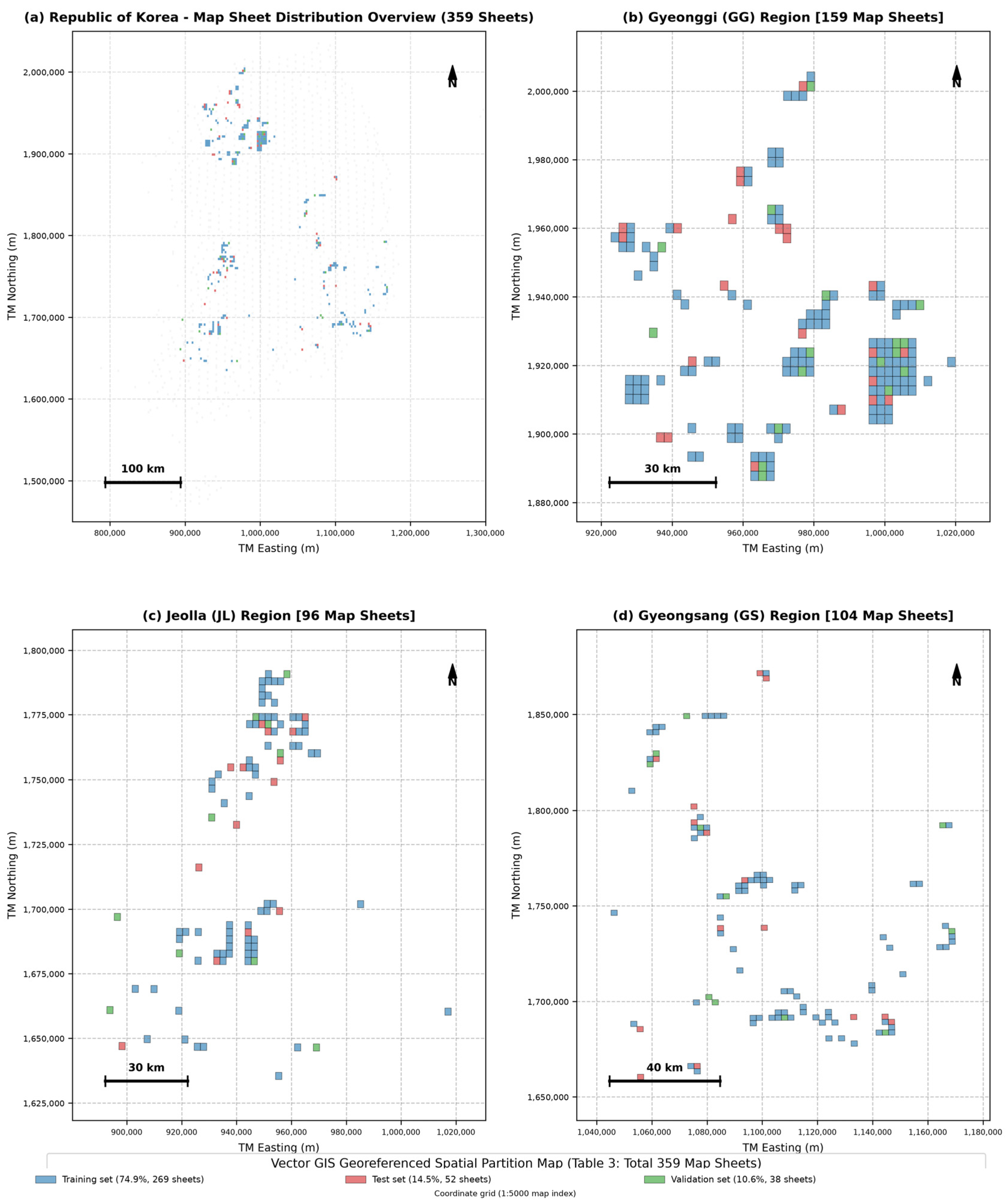
Spatial partitioning used the 1:5000 map sheet as the assignment unit. Every tile belonging to one sheet was assigned exclusively to training, testing, or validation. The 359 sheets comprised 159 in Gyeonggi, 104 in Gyeongsang, and 96 in Jeolla. Sheet counts were 269 training (74.9%), 52 testing (14.5%), and 38 validation (10.6%); the corresponding tile counts were 12,613 (81.2%), 1689 (10.9%), and 1233 (7.9%), respectively (
Table 3). Reporting both percentages avoids conflating the sheet-level allocation with the resulting tile-level distribution.
Figure 1 locates the represented regions and preserves the original partition symbols, with the numerical split counts stated explicitly. Symbol overlap in the embedded map cannot be used to estimate partition proportions. The split prevents the same map-sheet identifier from occurring in multiple partitions, but does not by itself eliminate neighboring-sheet dependence, selection bias, or other preprocessing dependencies.
3.2. Segmentation Models and Training
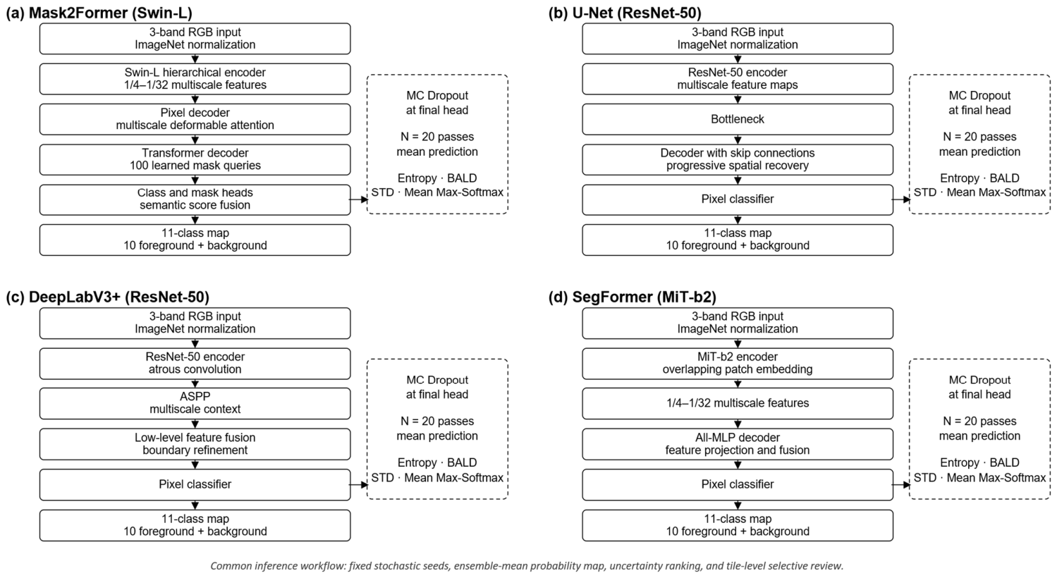
Four architectures were trained and evaluated using the same spatial partitions, loss framework, and augmentation policy (
Table 4). U-Net and DeepLabV3+ used ResNet-50 encoders pretrained on ImageNet-1K [
17,
18]. SegFormer used the ImageNet-1K-pretrained MiT-b2 encoder [
19]. Mask2Former used a Swin-L backbone initialized from ImageNet-22K and Cityscapes semantic-segmentation weights; its classification head was reinitialized for the 11 study classes [
20,
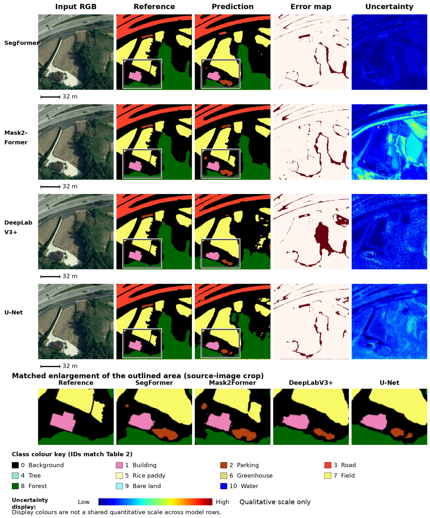
21]. The different parameter counts and pretraining sources were retained as conventional architecture configurations, so comparisons are descriptive benchmarks rather than capacity-matched ablations.
All models produced 11-class predictions, including the background class, which participated in the training objective. Following the original preprocessing workflow, one negative-log-frequency class-weight vector was calculated from the complete labeled-tile inventory and shared by all four architectures; each weight was clipped to the interval [0.1, 10.0]. The weight for class
was
where
is the number of labeled pixels used to calculate the shared weight for class
, and
. A weighted focal term was applied to the final semantic-probability map:
where
is the probability of class
at pixel
, and
is the corresponding one-hot target. The total objective combined the architecture-native loss and the auxiliary focal term:
For Mask2Former, comprised bipartite-matching classification, binary cross-entropy, and Dice components. For the three pixel-classification models, it was pixelwise cross-entropy. Focal loss was evaluated in an fp32 context under automatic mixed precision to maintain numerical stability.
Under the recorded complete-inventory weighting workflow, class-frequency information was not isolated to the training partition, even though model fitting used training tiles. This preprocessing dependency limits a strict leakage-free interpretation. A training-only recomputation of the weights and refitting would be required to establish its effect; that comparison is not part of the reported results.
The inference workflow contained an optional two-stage background rule. First, a raw class was obtained by maximization over all 11 classes:
The delivered class under the operational rule was then
Training used 512 × 512 inputs, AdamW optimization, a polynomial learning-rate schedule, automatic mixed precision, and gradient checkpointing. Augmentation reflected the orientation invariance of nadir imagery: horizontal and vertical flips were each applied with probability 0.5, rotation was randomly selected from 0°, 90°, 180°, and 270°, and brightness was multiplied by a factor sampled from 0.8–1.2. All architectures were trained for 100 epochs.
Figure 2 summarizes the architectures and the common stochastic-inference workflow.
3.4. Evaluation Protocol
3.4.1. Classification Metrics
Two mIoU quantities were retained because they were computed over different evaluation masks. Let
contain every valid pixel, and let
contain only pixels whose reference label is foreground. The primary metric was the 11-class mean over
; the complementary metric was computed after restricting the evaluation mask to
and averaging the ten foreground classes:
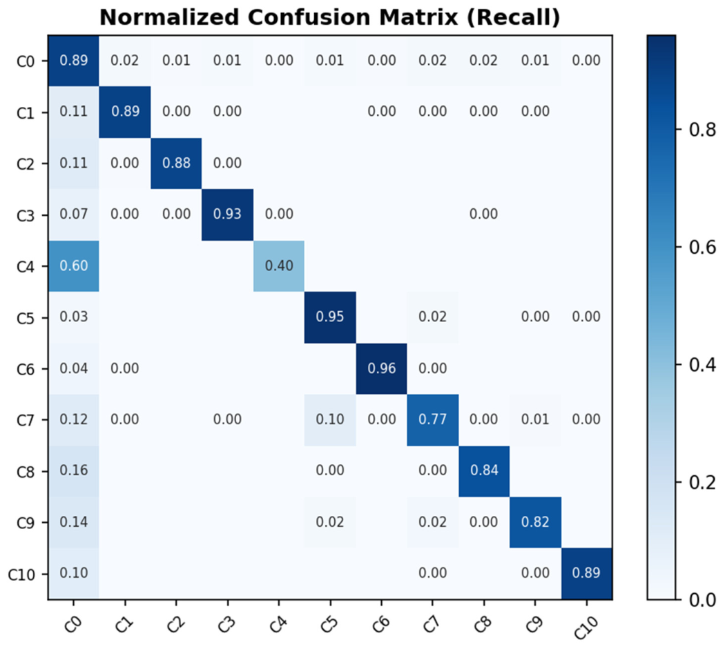
Because the second quantity excludes reference-background pixels before constructing its confusion statistics, it is not algebraically derivable from the first and is not labeled as a standard background-excluded mIoU. Overall accuracy, Cohen’s Kappa, macro-F1, and the primary mIoU were evaluated on .
In mapping terms, IoU measures the overlap between a predicted class and its reference extent, penalizing both missed and falsely assigned area. Restricting the mask to reference foreground removes opportunities to count false foreground assignments on reference background; the restricted score must therefore be interpreted alongside, not instead of, the all-valid-pixel score.
Per-class precision and recall were
The corresponding F1 score was
The relation between classwise IoU and F1 was
3.4.2. Error Detection, Sparsification, and Calibration
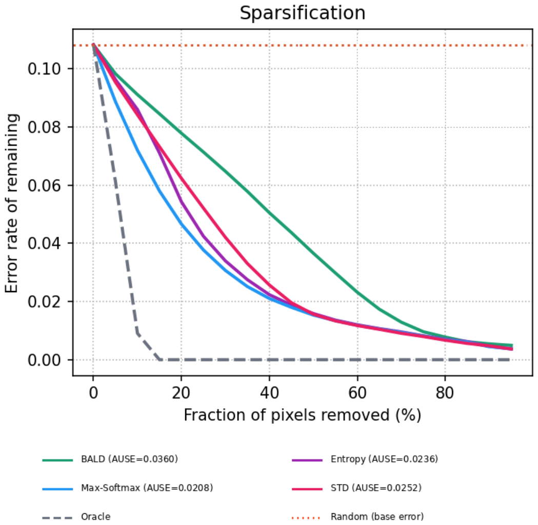
A pixel was an error when the unthresholded 11-class argmax prediction differed from the reference label. Uncertainty was used as the score for detecting this binary outcome. AUROC was reported together with AUPRC and the error base rate because errors were the minority class. Sparsification removed pixels in decreasing uncertainty order and compared the residual-error curve with an oracle ordering that removes actual errors first. The area between these curves is the area under the sparsification error (AUSE), for which smaller values are better.
For a map reviewer, AUROC describes how well a score places erroneous pixels ahead of correct pixels; 0.5 represents an uninformative ranking. It does not measure whether predicted probabilities are calibrated. AUPRC additionally reflects the prevalence of errors, so comparisons should retain the error base rate. Sparsification asks how much error remains after high-uncertainty pixels are set aside, and AUSE measures the gap from an ideal error-first ordering. These pixel-based diagnostics do not measure the time needed to inspect or edit a cartographic object.
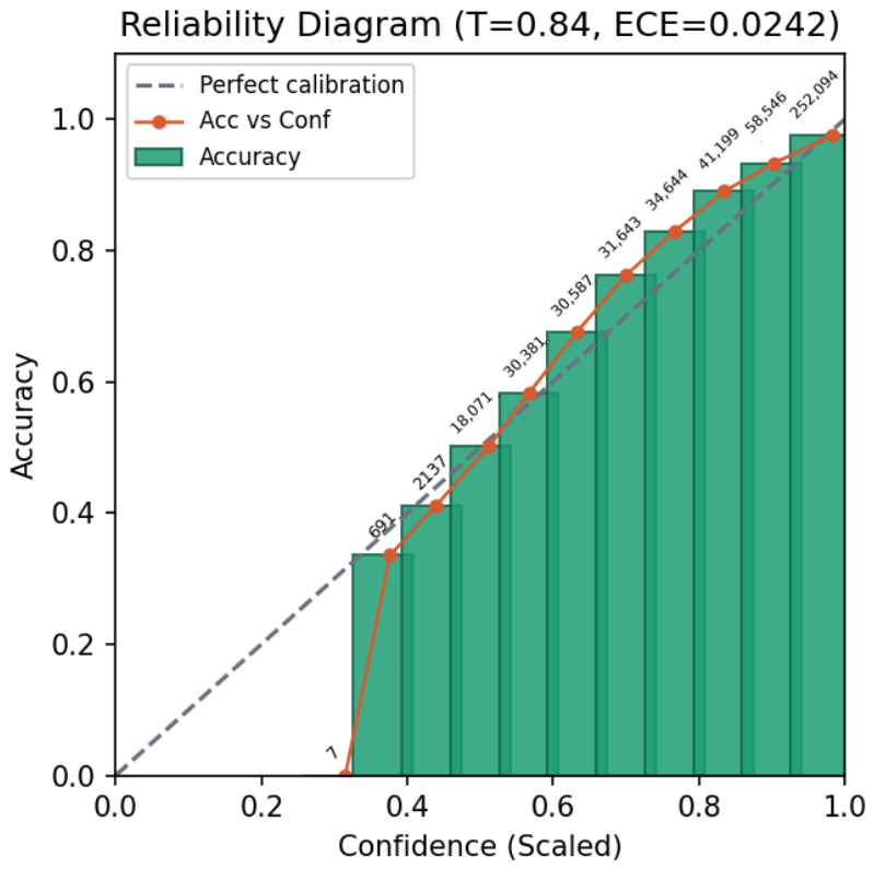
ECE used 15 equal-width confidence bins:
Temperature scaling fitted one scalar, to the validation-set NLL using bounded scalar optimization over [0.5, 5.0] with tolerance . The fitted temperature was then fixed for test-set evaluation. NLL and Brier score supplemented ECE.
ECE summarizes discrepancies between confidence and observed correctness within confidence bins. A low ECE alone does not imply high thematic accuracy or strong error ranking; NLL and Brier score provide complementary checks of probability quality.
3.4.3. Threshold-Decoupling Conditions
Three conditions were computed from the same probability tensors. Condition 1 used plain 11-class argmax without a confidence threshold. Condition 2 treated pixels below as an abstain state and evaluated accuracy only on accepted pixels. Condition 3 applied Equation (5) and reassigned below-threshold pixels to the background. Reporting these conditions separately tests whether the background rule mechanically creates the apparent relation between Max-Softmax uncertainty and error.
3.4.4. Reference-Conditioned and Prediction-Based Review Analyses
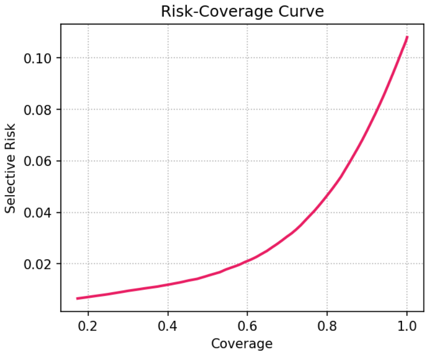
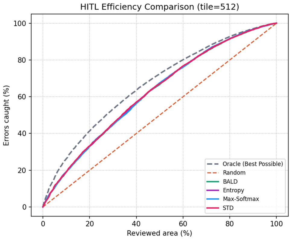
The recorded review simulation ranked 512 × 512 tiles by mean uncertainty over pixels labeled as foreground in the reference. The reviewed-area denominator was also the number of reference-foreground pixels, whereas recovered errors were counted over all valid pixels. Thus, reference labels influence both the inspection order and its cost normalization. The resulting 20% budget cannot be constructed by an operator who has no reference map. We retain these values only as retrospective, reference-conditioned diagnostics, not as operational savings or an estimate of how much of a complete map must be reviewed.
The recorded simulation compares the uncertainty curves with a nominal random diagonal and an oracle curve. With variable reference-foreground area per tile and an all-valid-pixel error numerator, a 20% area budget does not establish an empirical 20% random-order expectation. We therefore do not report lift over random as an operational effect size. Sensitivity analyses changed the review grid to 256 × 256 and replaced the tile mean with the median, 90th percentile, 95th percentile, or mean of the upper 10% of uncertainty values.
A separate prediction-based simulation formed the inspection queue from mean BALD over predicted-foreground pixels (pred ≠ 0), without reference labels. Reference labels were used only after the queue was frozen to score captured errors. Its reported 20% budget denotes the top 20% of the queue, rather than 20% of the reference-foreground area. Uniform random-order comparisons used 100 repetitions. The classwise counts are reported in the Discussion and interpreted in
Section 5.4. The two review analyses are interpreted separately because the equivalence of their evaluation inventories and error-counting domains is not established. Ranking only predicted foreground can miss foreground-to-background omissions, so a background audit or full-area coverage rule is also needed when adapting this protocol for deployment.
3.5. Reproducibility
The analysis used
MC samples, dropout probability 0.1, fixed stochastic seeds 1–20, focal-loss parameters
and
, class-weight clipping to [0.1, 10.0], background threshold 0.5, and 15 ECE bins. Model selection and temperature fitting used the validation partition, and the test partition was used for the reported final metrics and retrospective evaluation. The public QGIS-oriented implementation provides dataset loaders with separate train, validation, and test directories, training-only augmentation, model definitions, uncertainty analysis, and configuration support [
36].
Reproduction of the reported experiment additionally requires the exact retained-file and split manifests, screening log, class-weight vector, training configuration, model checkpoints, and prediction/uncertainty exports linked to a fixed code revision. A publicly accessible software repository is not, by itself, a versioned archive of these experimental artifacts. The reported intervals and comparisons remain conditional on the recorded trained models and evaluation outputs.