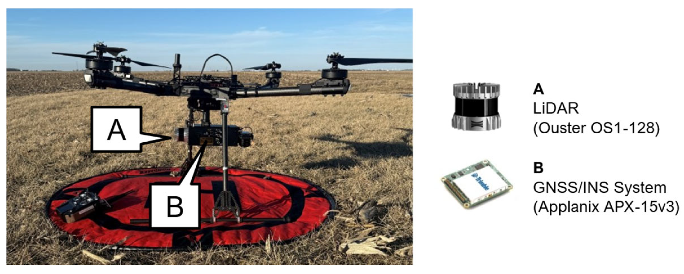
Figure 1.
UAV LiDAR system with its sensing and georeferencing components.
Figure 1.
UAV LiDAR system with its sensing and georeferencing components.
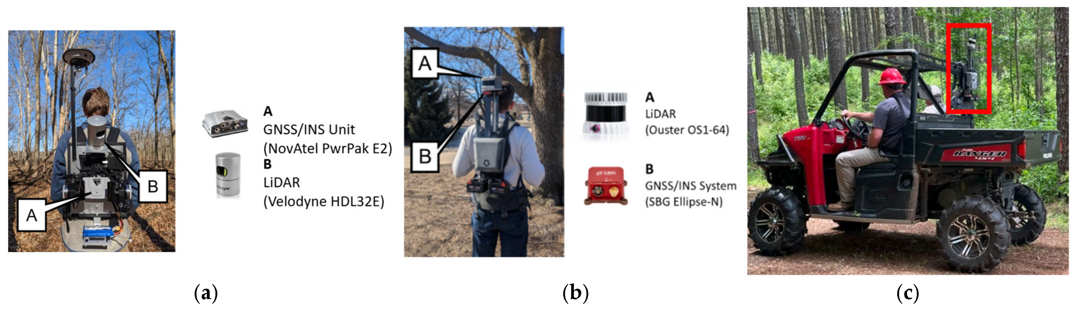
Figure 2.
Illustration of BackPack systems with their sensing and georeferencing components: (a) E2HDL32E, (b) Knap-XP1, and (c) ATV Knap-XP1 systems.
Figure 2.
Illustration of BackPack systems with their sensing and georeferencing components: (a) E2HDL32E, (b) Knap-XP1, and (c) ATV Knap-XP1 systems.
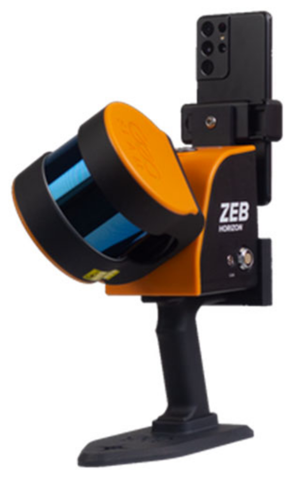
Figure 3.
Handheld (GeoSLAM Horizon RT) LiDAR system.
Figure 3.
Handheld (GeoSLAM Horizon RT) LiDAR system.
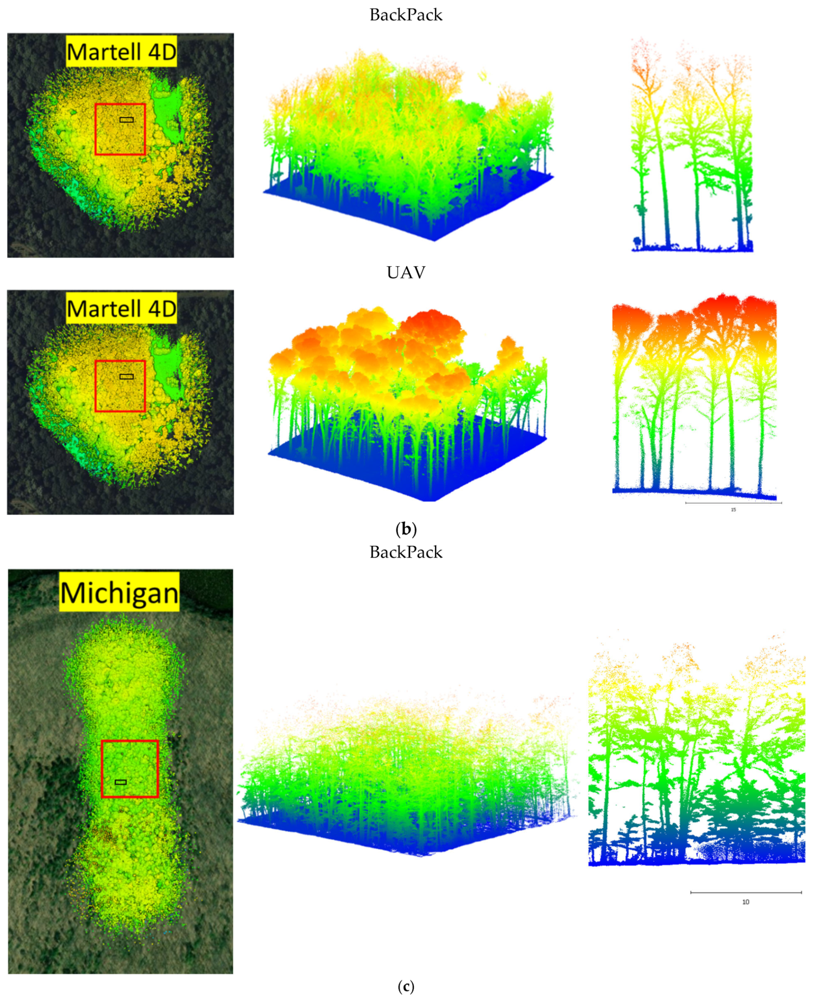
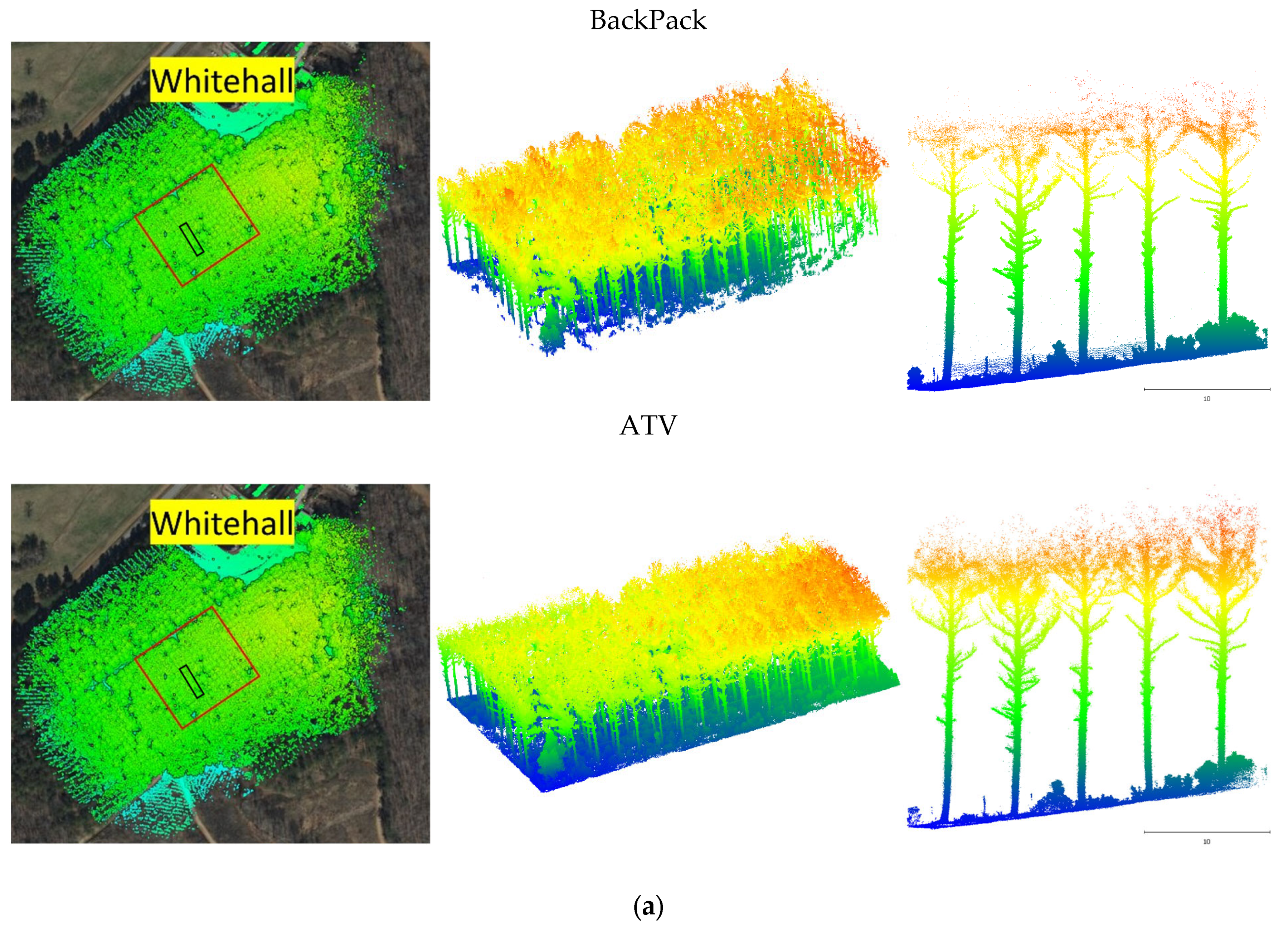
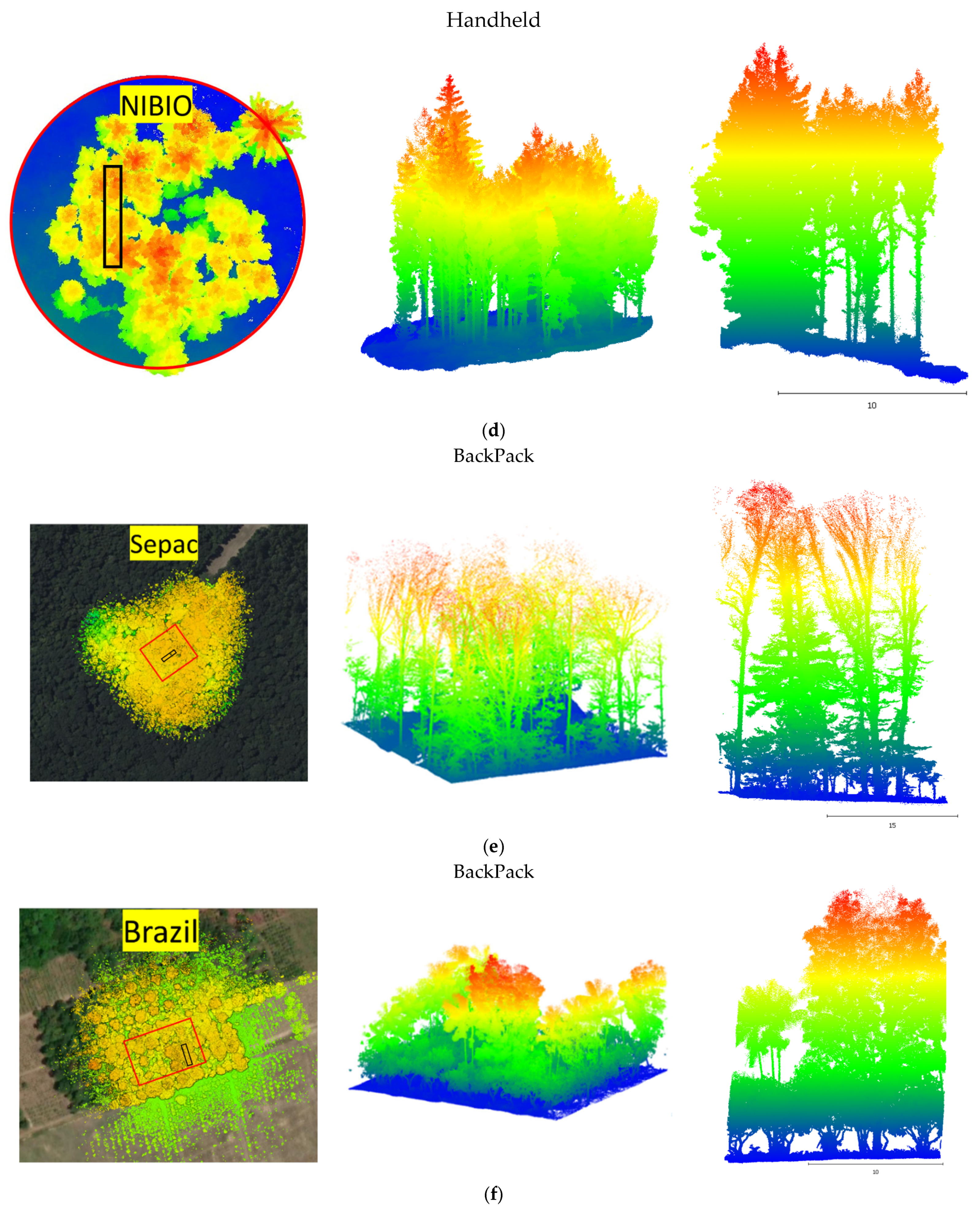
Figure 4.
Illustrations of the study sites and evaluation ROIs. For each site, (left) shows the point cloud colored by height with the ROI boundary in red and the location of the representative profile in black, (middle) the extracted ROI point cloud, (right) and the corresponding profile with a scale bar: (a) Whitehall, (b) Martell 4D, (c) Michigan, (d) NIBIO, (e) SEPAC, and (f) Brazil.
Figure 4.
Illustrations of the study sites and evaluation ROIs. For each site, (left) shows the point cloud colored by height with the ROI boundary in red and the location of the representative profile in black, (middle) the extracted ROI point cloud, (right) and the corresponding profile with a scale bar: (a) Whitehall, (b) Martell 4D, (c) Michigan, (d) NIBIO, (e) SEPAC, and (f) Brazil.
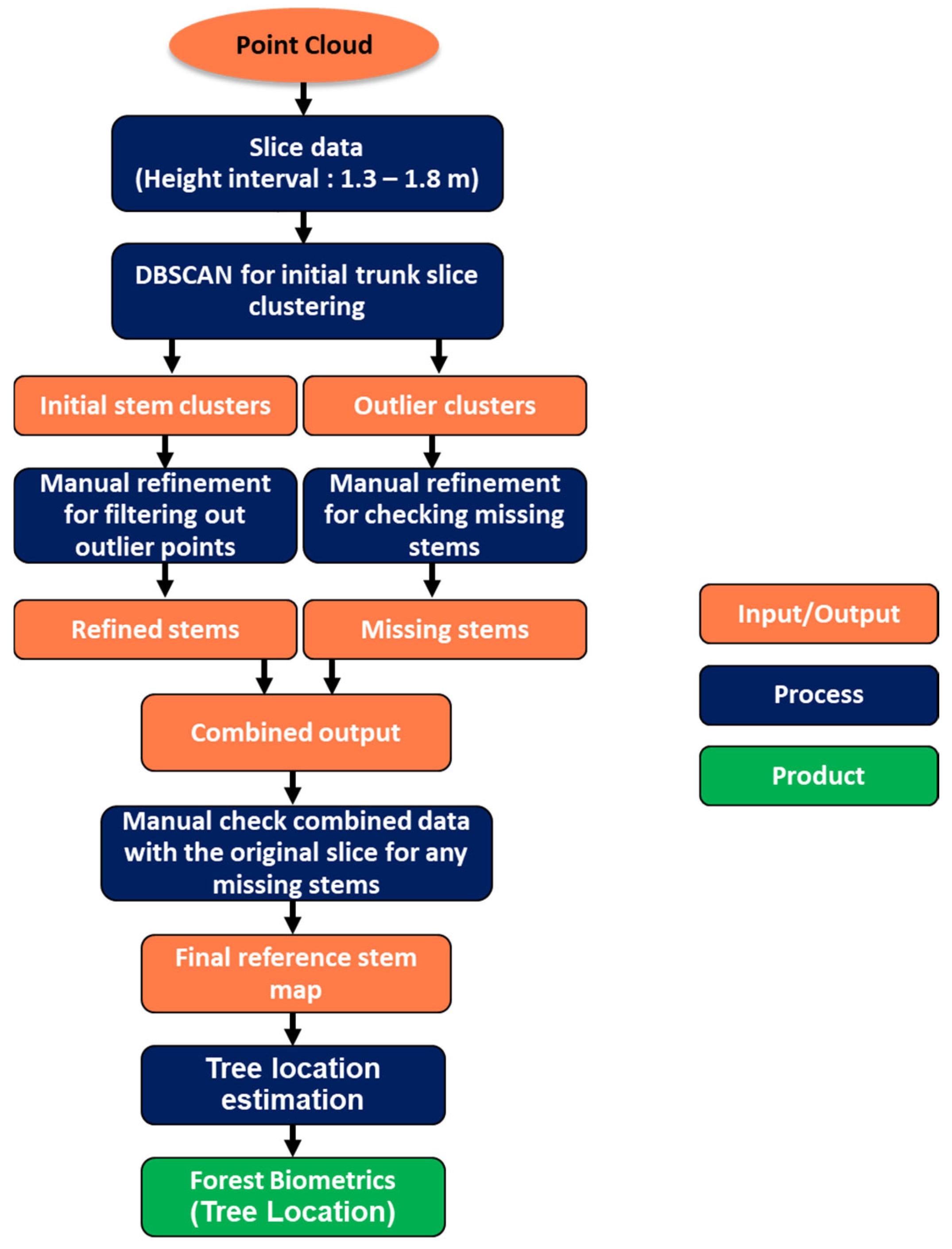
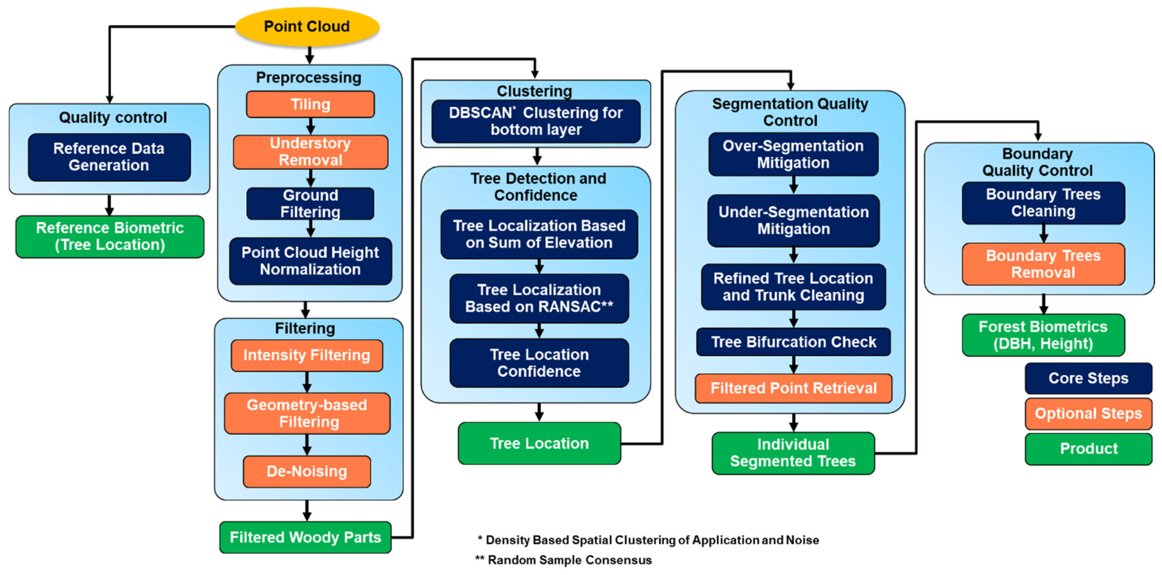
Figure 5.
Workflow for proposed forest biometrics derivation pipeline.
Figure 5.
Workflow for proposed forest biometrics derivation pipeline.
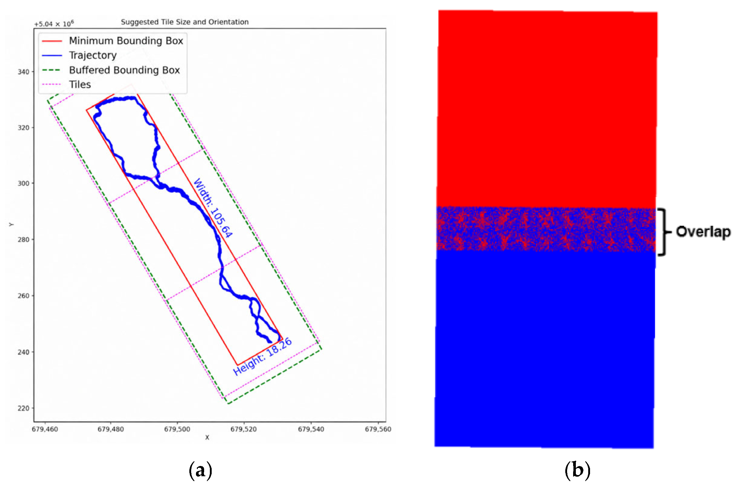
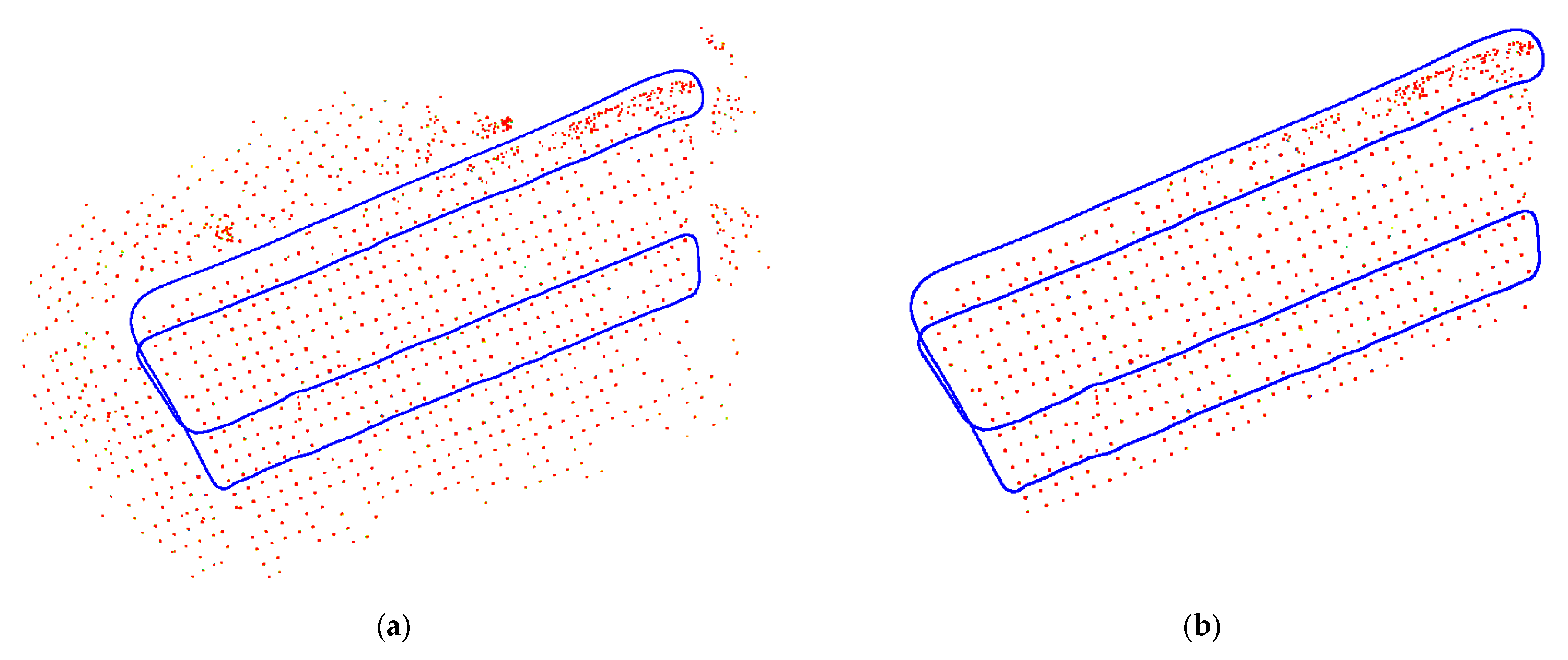
Figure 6.
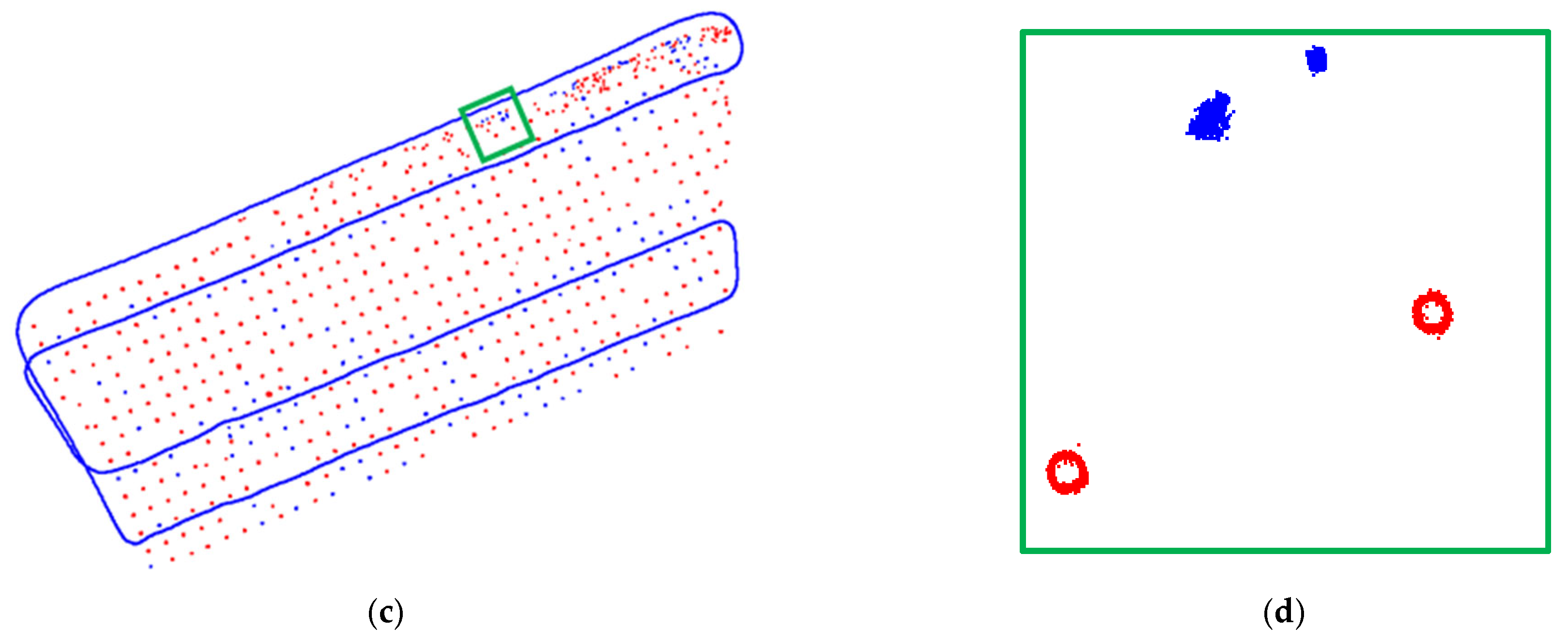
An illustration of the tiling process: (a) the trajectory with the defined minimum bounding box and tile orientation, and (b) two adjacent tiles with their overlapping region highlighted.
Figure 6.
An illustration of the tiling process: (a) the trajectory with the defined minimum bounding box and tile orientation, and (b) two adjacent tiles with their overlapping region highlighted.
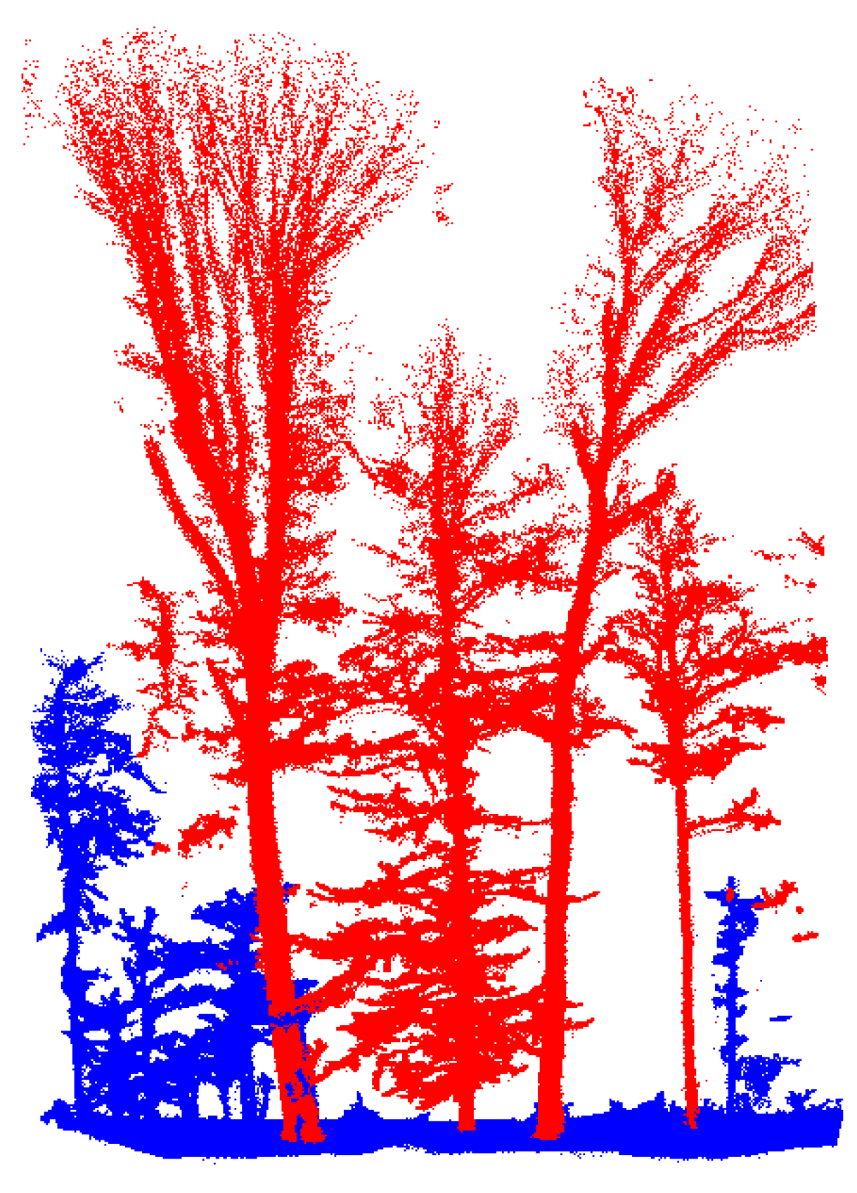
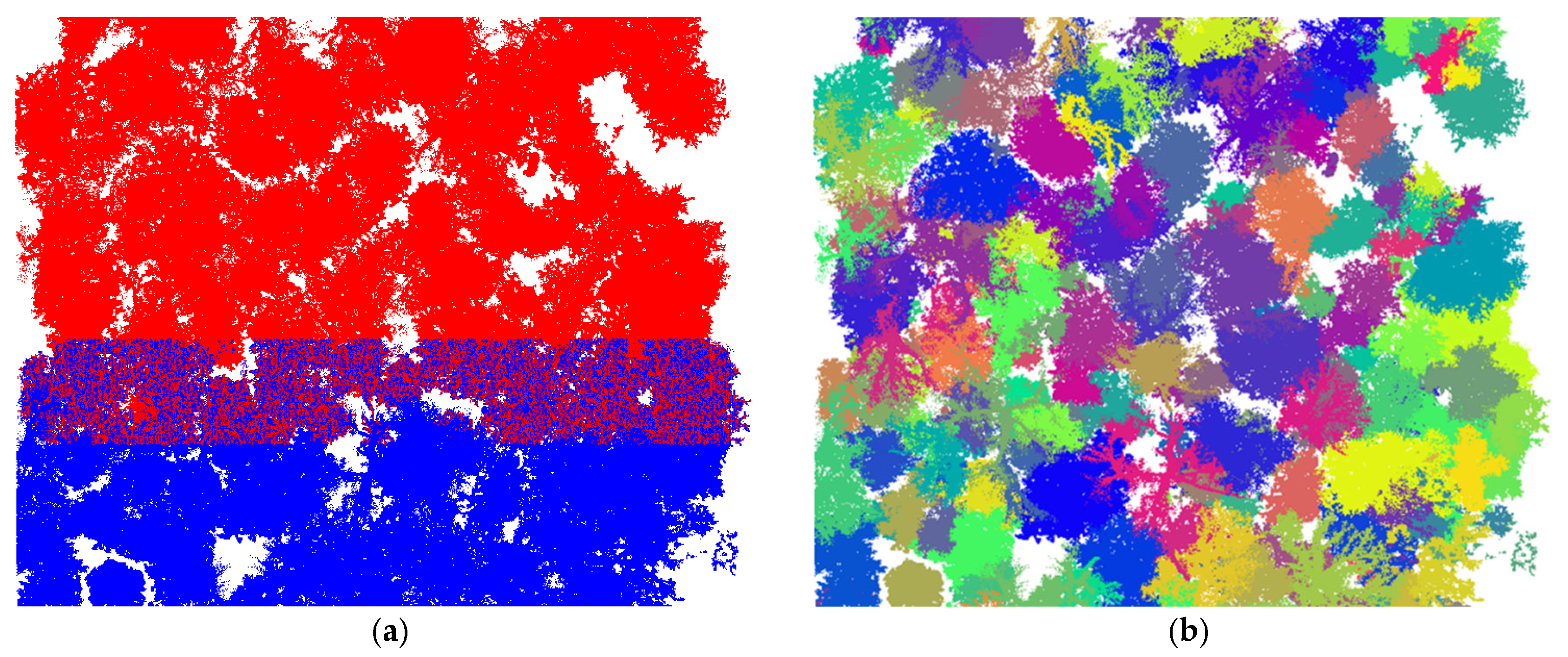
Figure 7.
An illustration of classified point cloud into overstory trees (in red) and understory vegetation (in blue).
Figure 7.
An illustration of classified point cloud into overstory trees (in red) and understory vegetation (in blue).
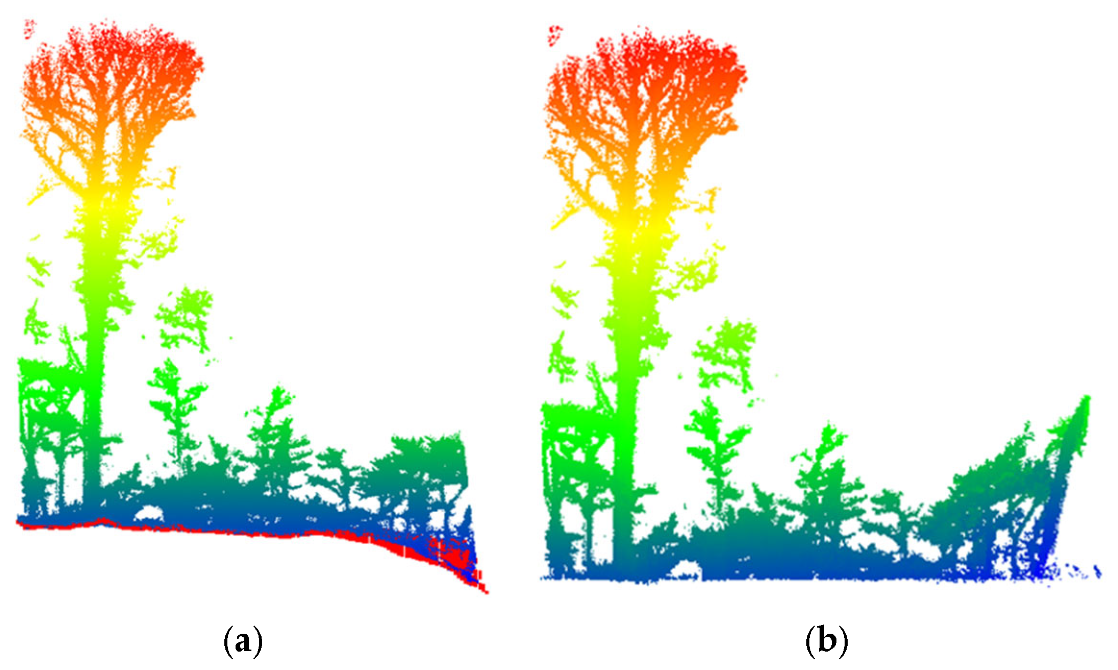
Figure 8.
An illustration of point cloud height normalization process: (a) original point cloud colored by height with the DTM in red, and (b) normalized height point cloud.
Figure 8.
An illustration of point cloud height normalization process: (a) original point cloud colored by height with the DTM in red, and (b) normalized height point cloud.
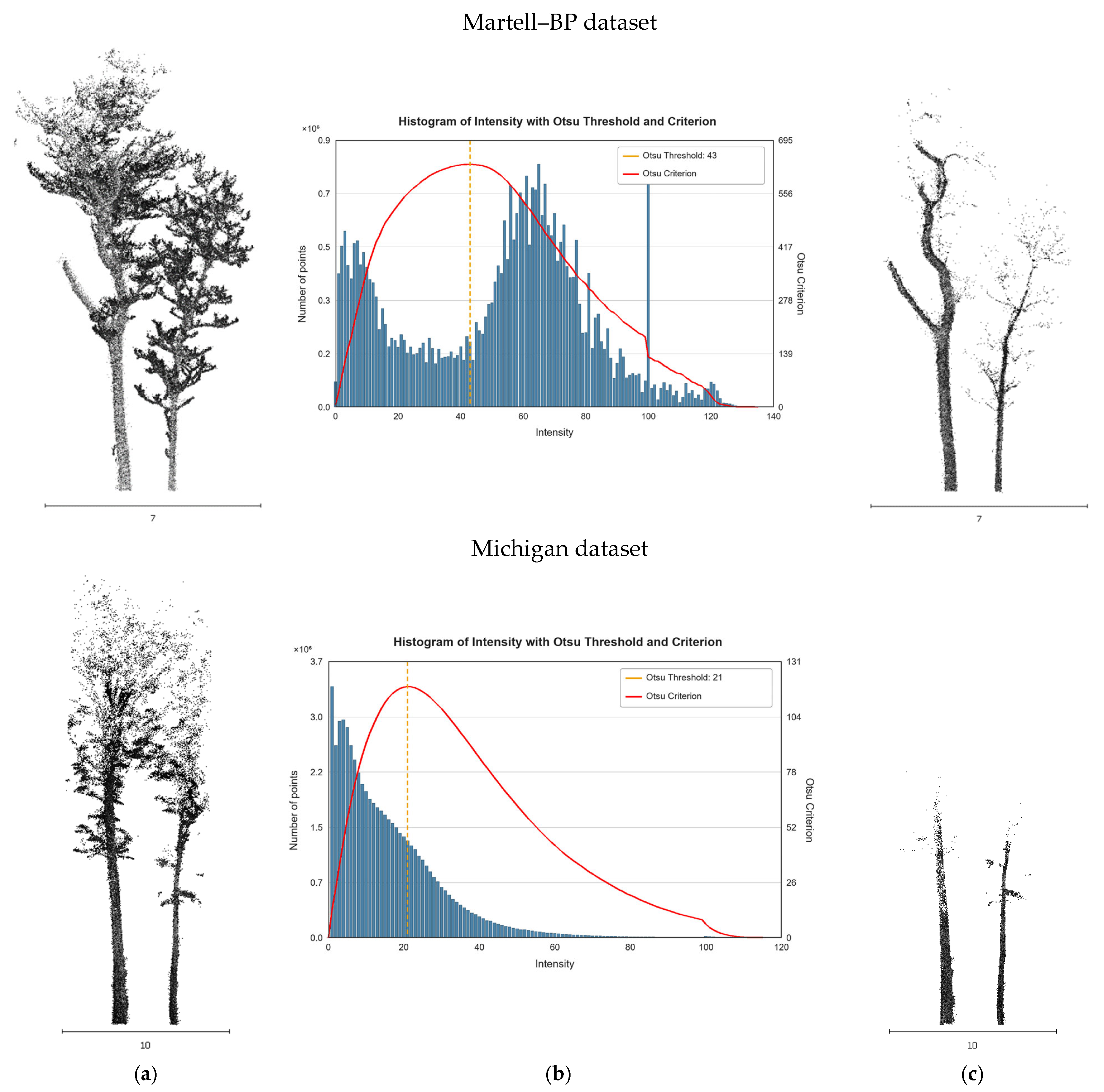
Figure 9.
An illustration of automated intensity thresholding for separating woody parts from foliage for the Martell–BP dataset (top row) and Michigan dataset (bottom row), where the point clouds visualizations are colored by intensity: (a) original tree before filtering, (b) intensity histogram with the Otsu threshold used to separate woody parts from foliage, and (c) isolated woody parts after intensity filtering.
Figure 9.
An illustration of automated intensity thresholding for separating woody parts from foliage for the Martell–BP dataset (top row) and Michigan dataset (bottom row), where the point clouds visualizations are colored by intensity: (a) original tree before filtering, (b) intensity histogram with the Otsu threshold used to separate woody parts from foliage, and (c) isolated woody parts after intensity filtering.
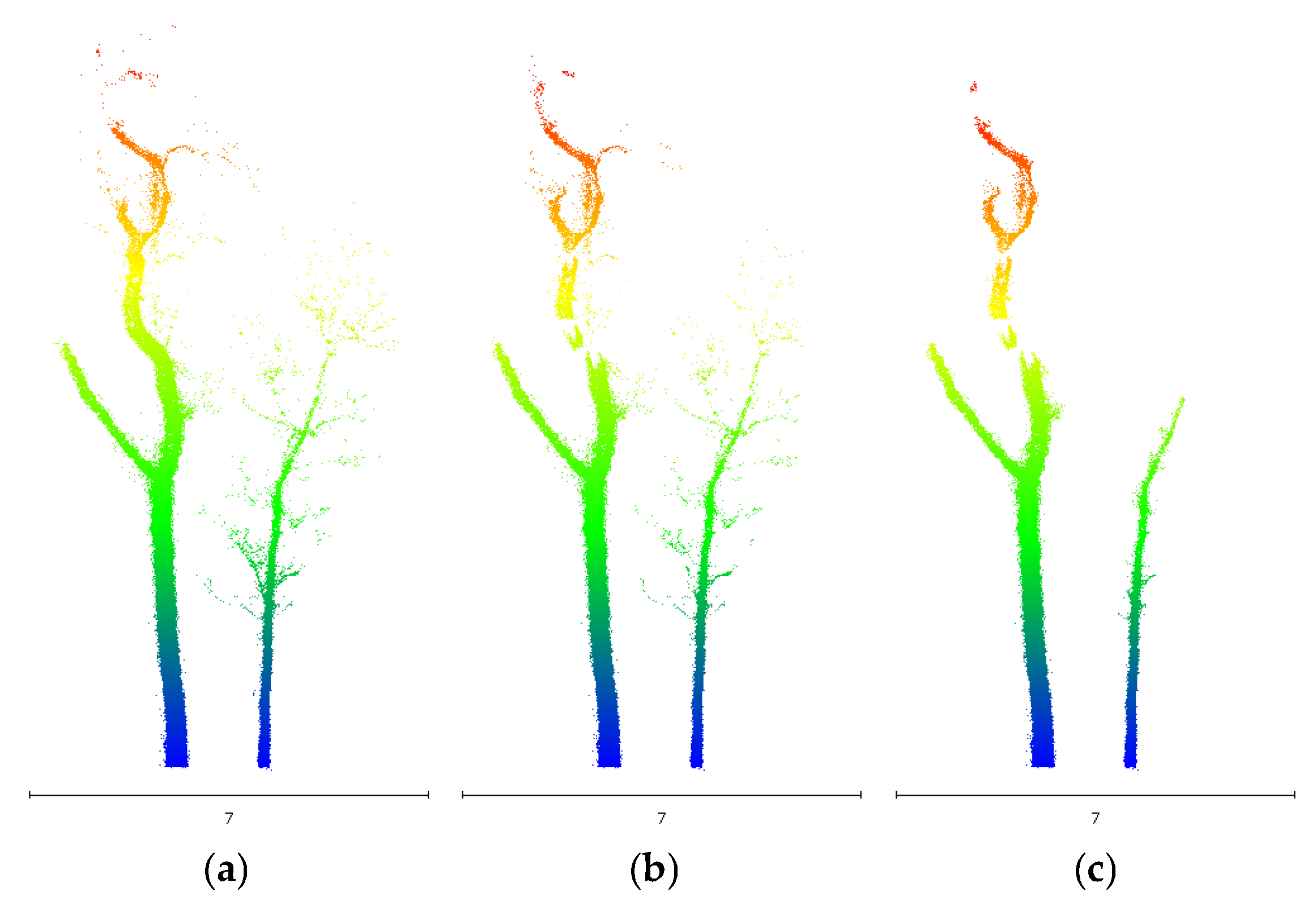
Figure 10.
An illustration of sequential woody part isolation results where the point cloud visualizations are colored by height: (a) isolated tree woody parts after intensity filtering, (b) isolated points with a high linearity metric, and (c) after SOR denoising.
Figure 10.
An illustration of sequential woody part isolation results where the point cloud visualizations are colored by height: (a) isolated tree woody parts after intensity filtering, (b) isolated points with a high linearity metric, and (c) after SOR denoising.
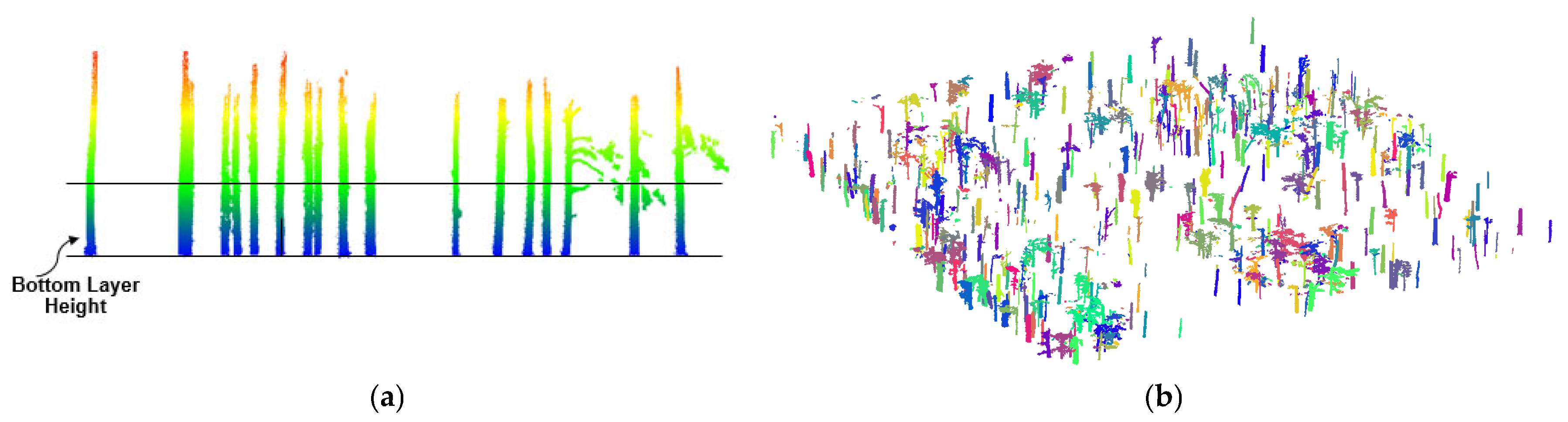
Figure 11.
Illustration of point cloud clustering process: (a) point cloud after all filtering steps applied colored by height, and (b) potential tree trunk clusters colored by cluster id.
Figure 11.
Illustration of point cloud clustering process: (a) point cloud after all filtering steps applied colored by height, and (b) potential tree trunk clusters colored by cluster id.
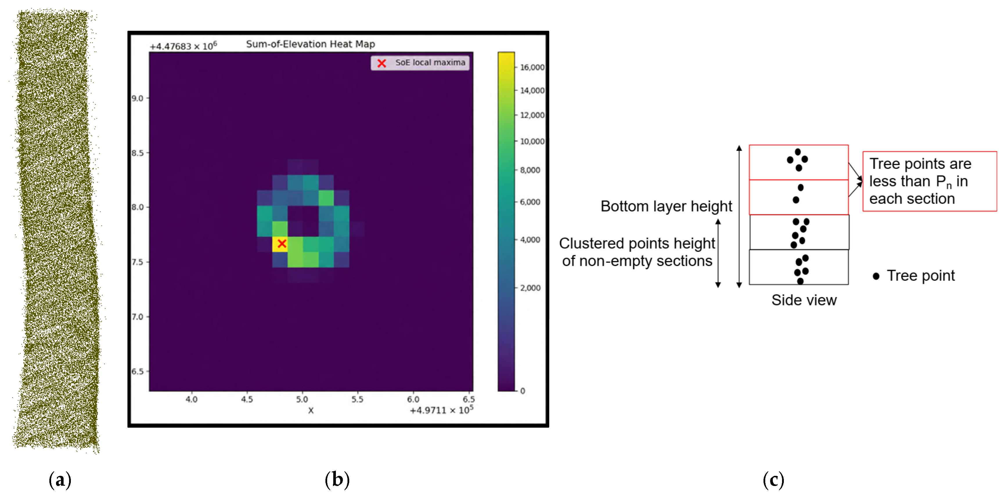
Figure 12.
An illustration of the SoE-based tree localization process: (a) sample tree trunk cluster used for tree detection colored by cluster id, (b) SoE heat maps generated for the sample cluster, where yellow indicates higher accumulated elevation values, and (c) partitioned clusters used for continuity and height checks.
Figure 12.
An illustration of the SoE-based tree localization process: (a) sample tree trunk cluster used for tree detection colored by cluster id, (b) SoE heat maps generated for the sample cluster, where yellow indicates higher accumulated elevation values, and (c) partitioned clusters used for continuity and height checks.
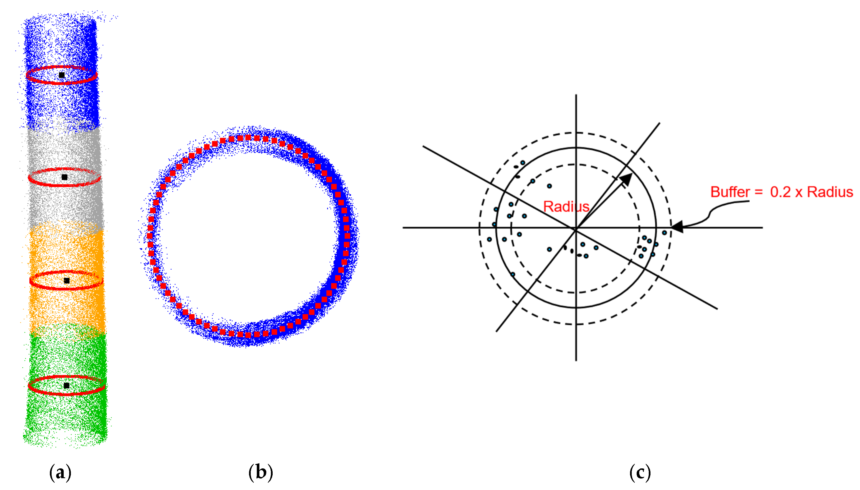
Figure 13.
An illustration of the RANSAC-based circle fitting localization method: (a) vertically sliced sections randomly colored with fitted circle (in red) and circle center (in black), (b) sample cross-section with fitted circle (in red), and (c) angular sectors used for cross-section completeness estimation.
Figure 13.
An illustration of the RANSAC-based circle fitting localization method: (a) vertically sliced sections randomly colored with fitted circle (in red) and circle center (in black), (b) sample cross-section with fitted circle (in red), and (c) angular sectors used for cross-section completeness estimation.
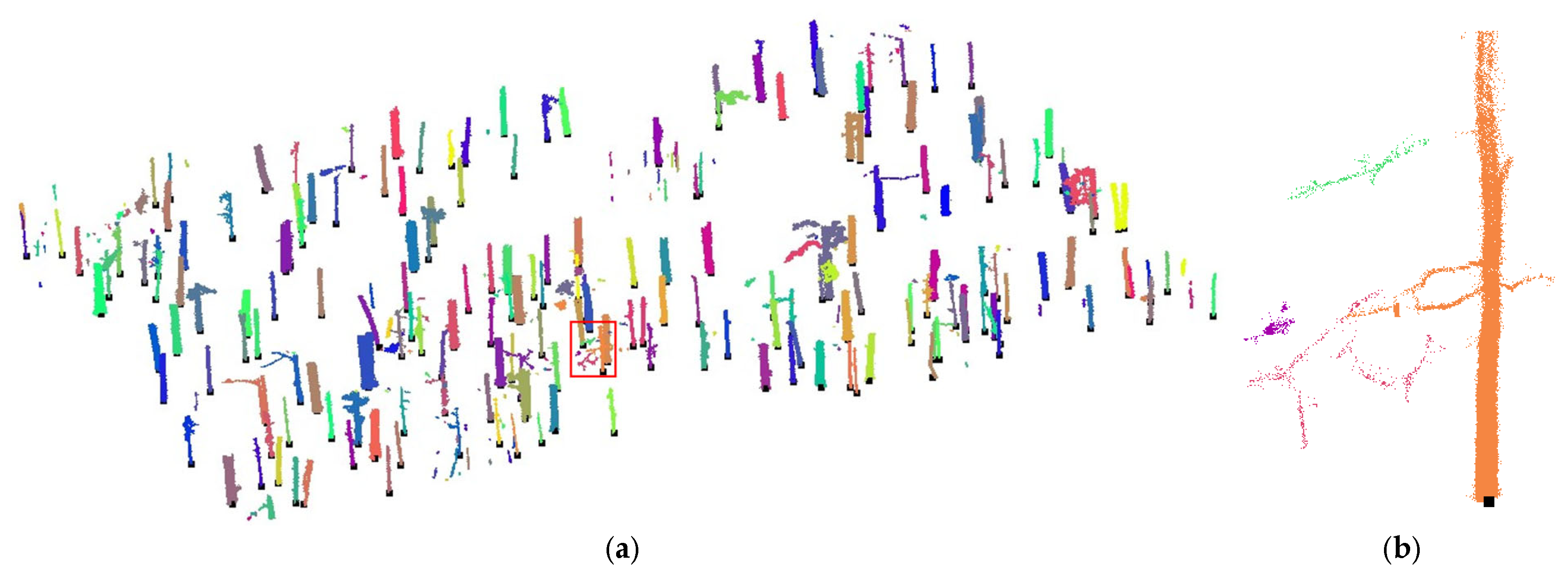
Figure 14.
An illustration of the quality control step for over-segmentation: (a) initial stem clusters overlaid with detected tree locations (in black); the red box indicates the region enlarged in panel (b) with zoom-in view for an over-segmented tree cluster.
Figure 14.
An illustration of the quality control step for over-segmentation: (a) initial stem clusters overlaid with detected tree locations (in black); the red box indicates the region enlarged in panel (b) with zoom-in view for an over-segmented tree cluster.
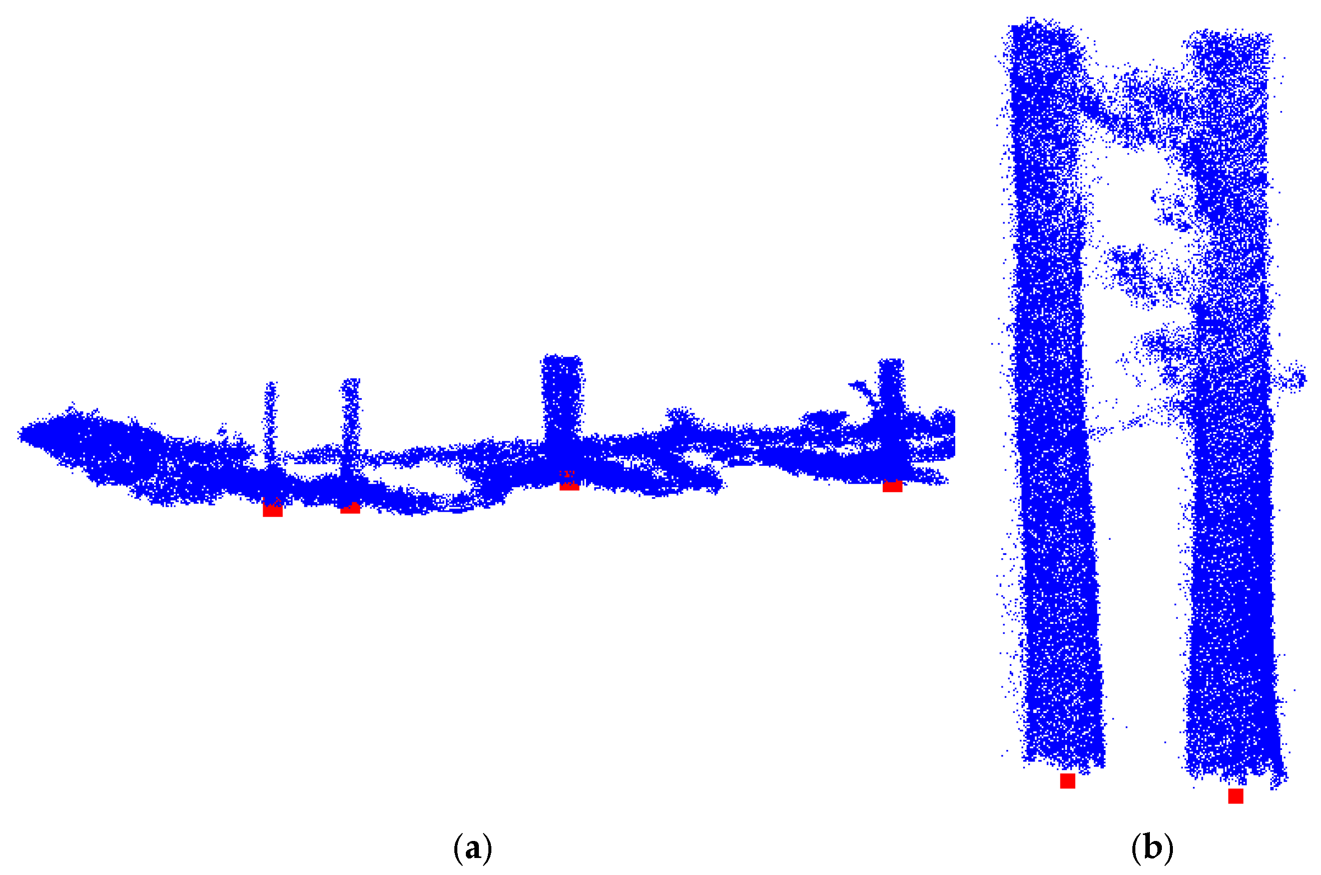
Figure 15.
Illustration of under-segmentation cases with large 2D extents (in blue) and multiple detected tree locations (in red): (a) an example of multiple trees grouped within a single cluster, and (b) an example where neighboring trunks become connected in the upper section.
Figure 15.
Illustration of under-segmentation cases with large 2D extents (in blue) and multiple detected tree locations (in red): (a) an example of multiple trees grouped within a single cluster, and (b) an example where neighboring trunks become connected in the upper section.
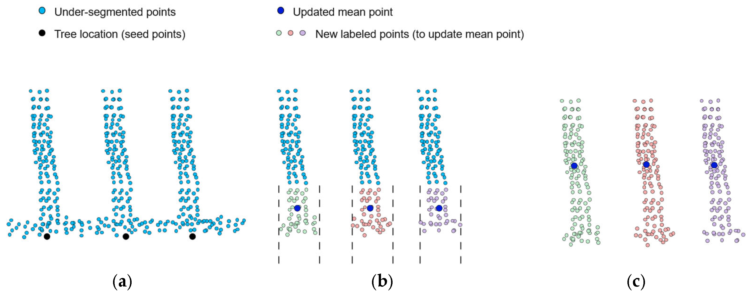
Figure 16.
An illustration of the bottom–up splitting process for an under-segmented cluster: (a) an under-segmented cluster with tree locations (in black), (b) the iterative process for splitting the cluster, and (c) the final clustered tree trunks.
Figure 16.
An illustration of the bottom–up splitting process for an under-segmented cluster: (a) an under-segmented cluster with tree locations (in black), (b) the iterative process for splitting the cluster, and (c) the final clustered tree trunks.
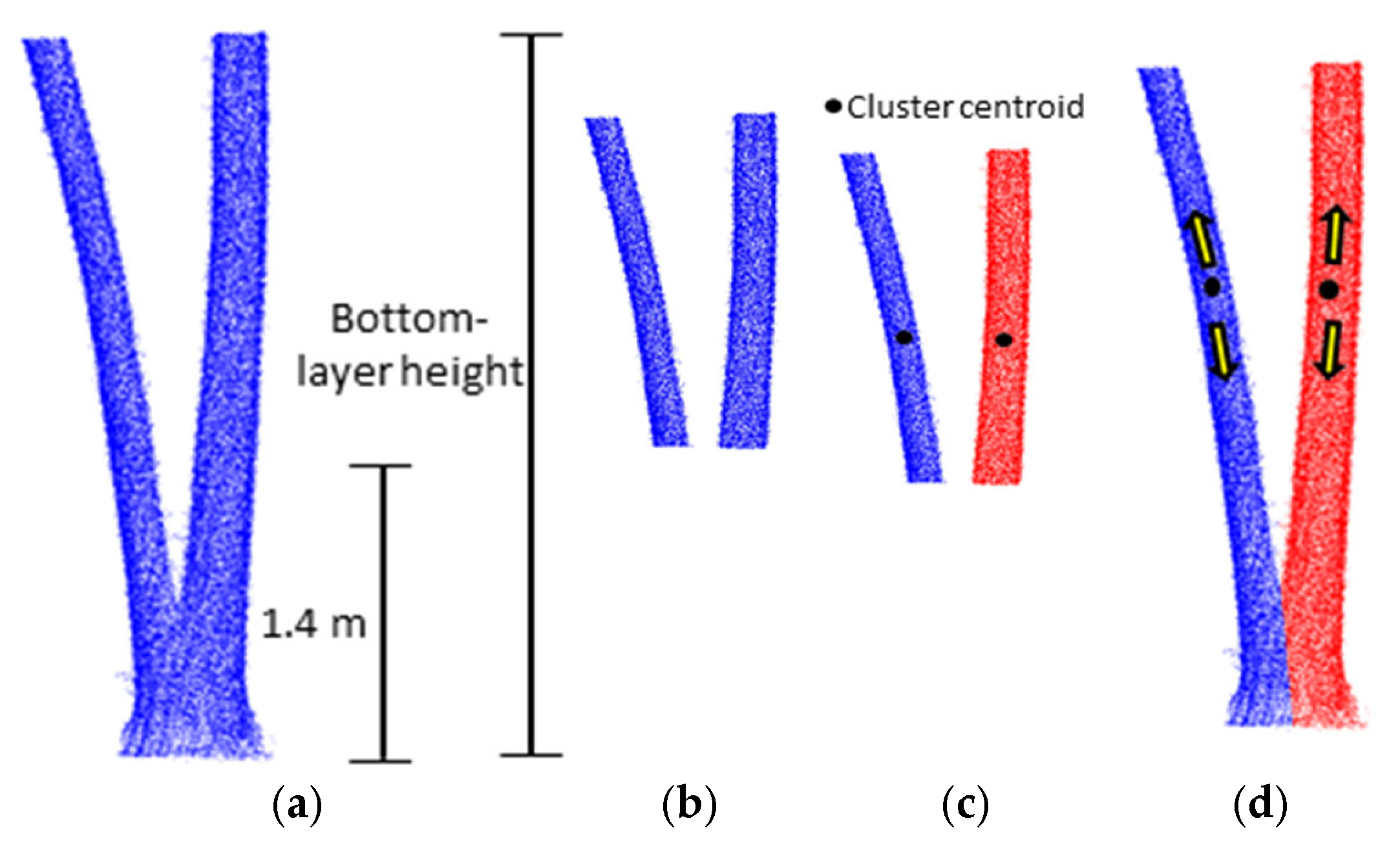
Figure 17.
Illustration of multi-stem quality control steps: (a) sample multi-stemmed tree, (b) cropped section for DBSCAN clustering, (c) clustered section with centroids (in black), and (d) isolated tree trunks after region growing with arrows showing bidirectional growth from each centroid.
Figure 17.
Illustration of multi-stem quality control steps: (a) sample multi-stemmed tree, (b) cropped section for DBSCAN clustering, (c) clustered section with centroids (in black), and (d) isolated tree trunks after region growing with arrows showing bidirectional growth from each centroid.
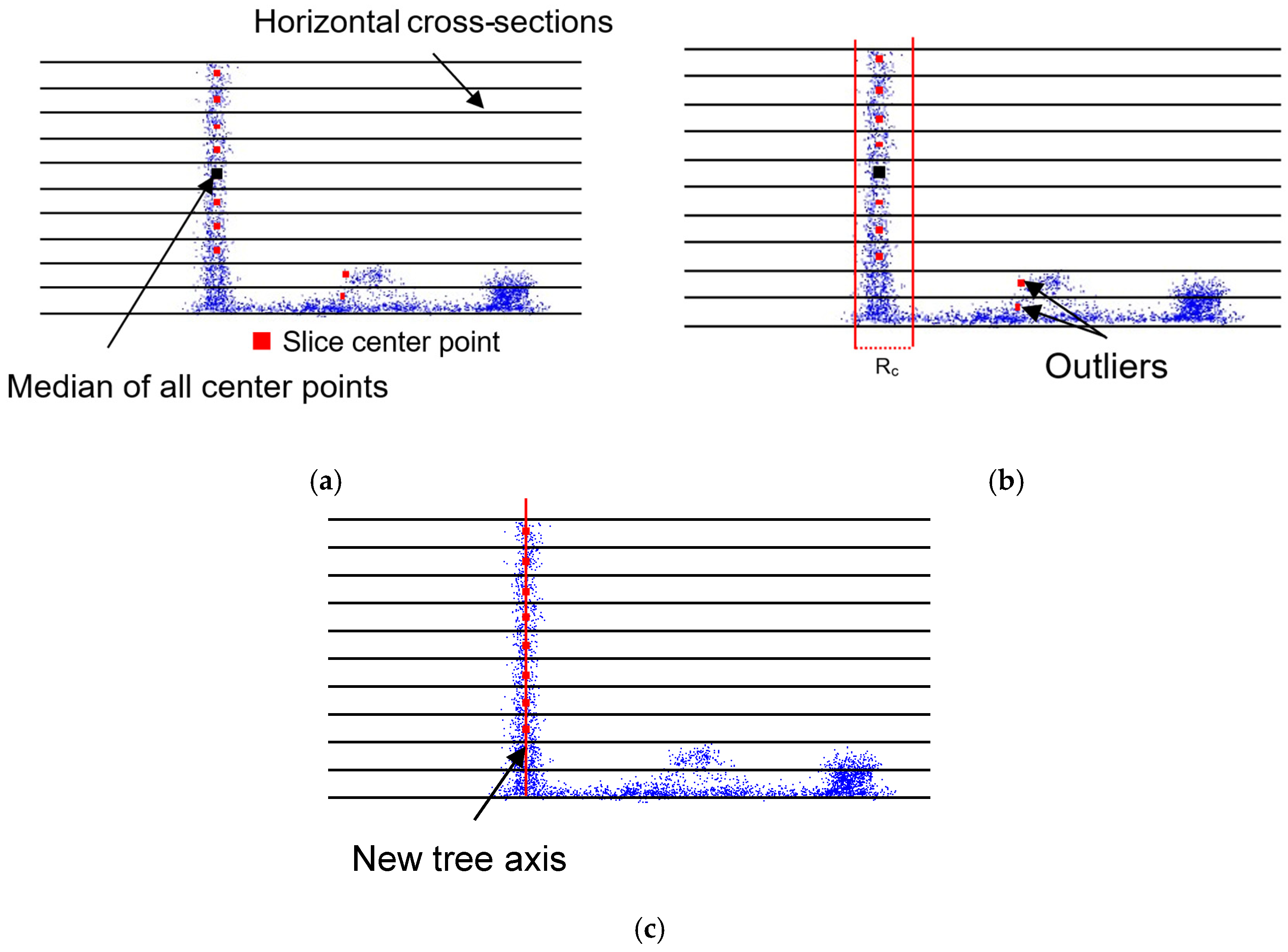
Figure 18.
An illustration of the trunk axis refinement process: (a) slice center (in red) estimates obtained from the horizontal cross-sections, with the median point (in black), (b) identification of outlier centers, where the two red lines indicate the threshold boundaries and (c) the final tree axis defined from the remaining inlier centers (in red).
Figure 18.
An illustration of the trunk axis refinement process: (a) slice center (in red) estimates obtained from the horizontal cross-sections, with the median point (in black), (b) identification of outlier centers, where the two red lines indicate the threshold boundaries and (c) the final tree axis defined from the remaining inlier centers (in red).
Figure 19.
An illustration of the filtered-point retrieval process with clustered stem (in black) and filtered points (in green): (a) vertical slicing used for filtered point retrieval, and (b) incremental retrieval of filtered points for neighboring interlocked trees.
Figure 19.
An illustration of the filtered-point retrieval process with clustered stem (in black) and filtered points (in green): (a) vertical slicing used for filtered point retrieval, and (b) incremental retrieval of filtered points for neighboring interlocked trees.
Figure 20.
Illustration of boundary cleaning step for abnormal retrieved trees: (a) point cloud with the abnormal tree example highlighted by the red box, and (b) the corresponding abnormal retrieved tree shown in detail.
Figure 20.
Illustration of boundary cleaning step for abnormal retrieved trees: (a) point cloud with the abnormal tree example highlighted by the red box, and (b) the corresponding abnormal retrieved tree shown in detail.
Figure 21.
An illustration of the abnormal-tree refinement step: (a) the height-dependent growing filter method used, and (b) an example showing the abnormal retrieved tree before refinement (left), isolating trunk points (in red) from foliage (in blue) (middle), and the final cluster after refinement (right).
Figure 21.
An illustration of the abnormal-tree refinement step: (a) the height-dependent growing filter method used, and (b) an example showing the abnormal retrieved tree before refinement (left), isolating trunk points (in red) from foliage (in blue) (middle), and the final cluster after refinement (right).
Figure 22.
Illustration of tile-overlap duplicate tree removal: (a) two overlapped tiles colored by tile id, and (b) tiles after removing duplicated trees colored by tree id.
Figure 22.
Illustration of tile-overlap duplicate tree removal: (a) two overlapped tiles colored by tile id, and (b) tiles after removing duplicated trees colored by tree id.
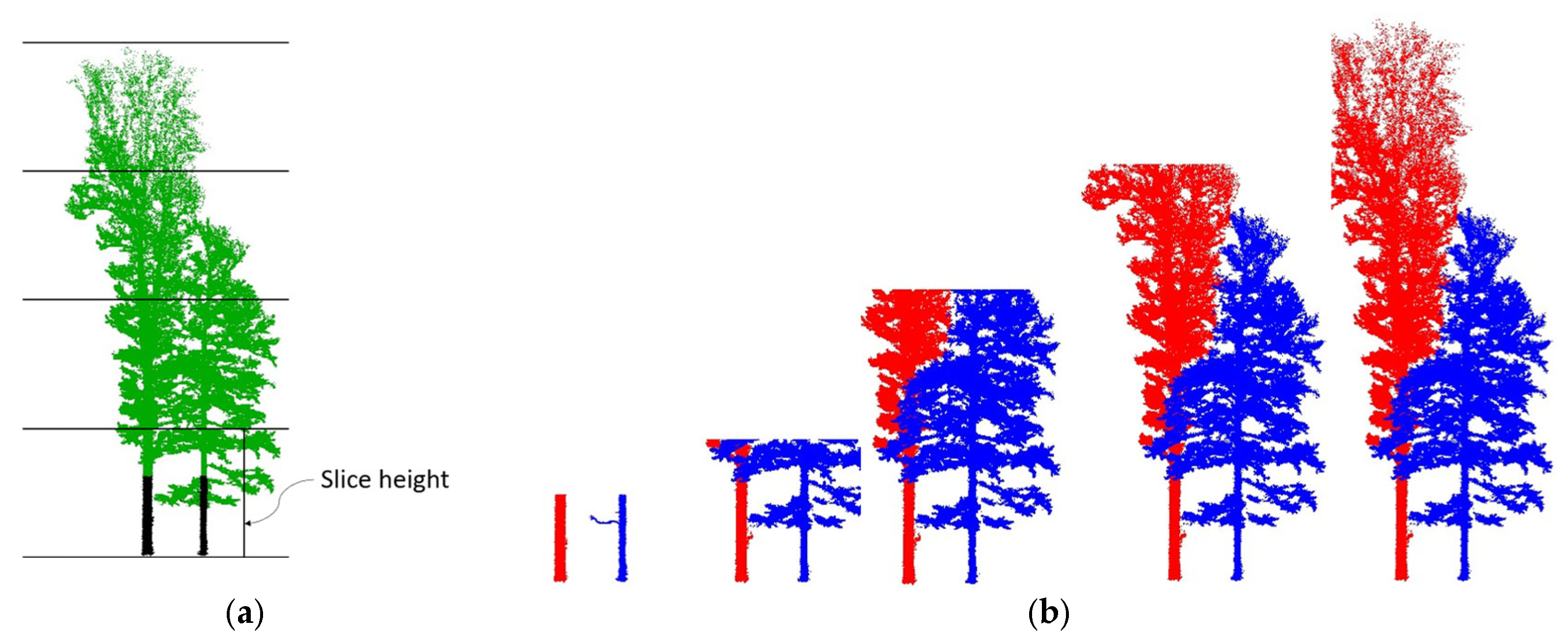
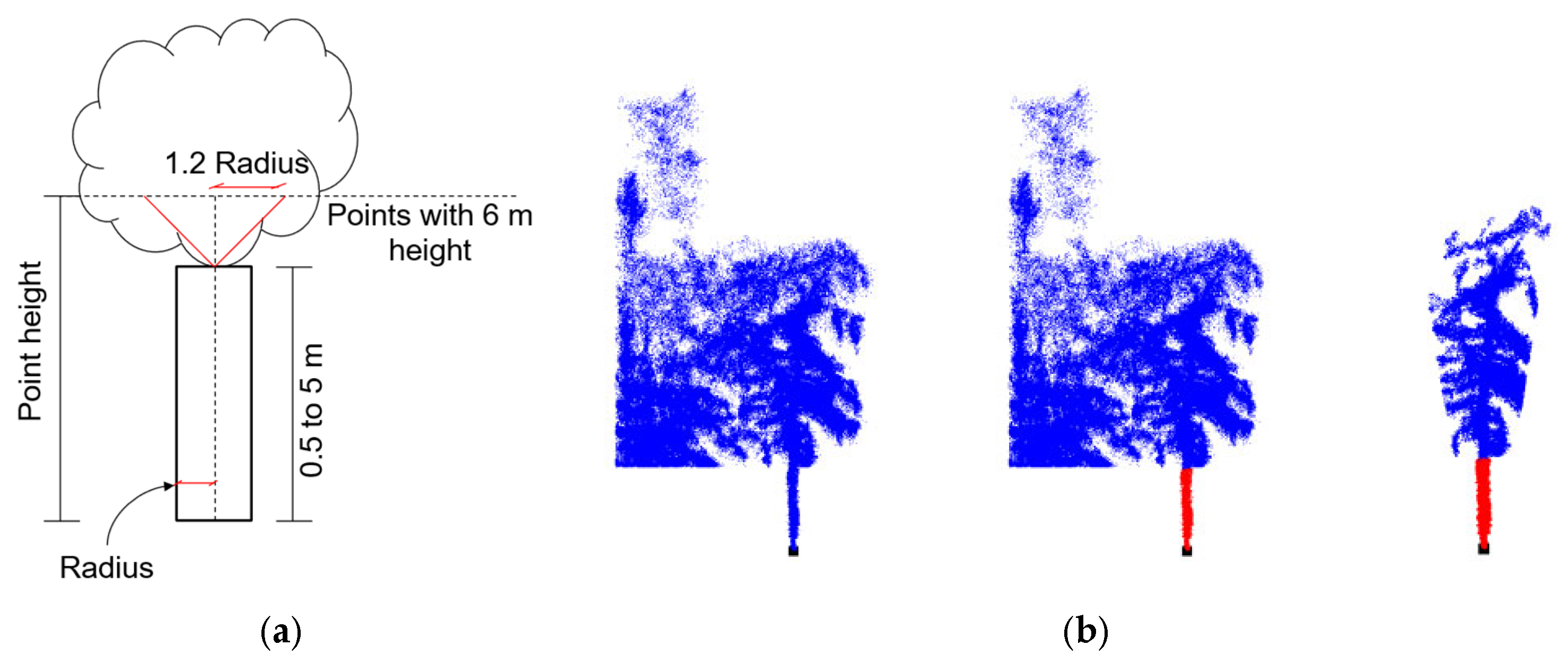
Figure 23.
Workflow for generating reference stem dataset and associated tree locations.
Figure 23.
Workflow for generating reference stem dataset and associated tree locations.
Figure 24.
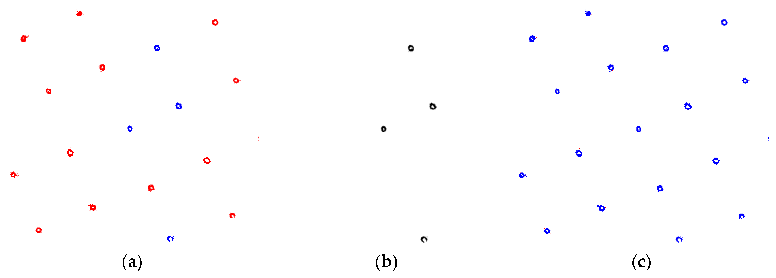
Normalized breast height slice used for initial stem clustering: (a) original sliced data colored by height with trajectory in blue, (b) sliced point cloud after ROI cropping using trajectory buffer, and (c) initial stem clusters (in red) and outlier clusters (in blue) shown in zoom-in window (d).
Figure 24.
Normalized breast height slice used for initial stem clustering: (a) original sliced data colored by height with trajectory in blue, (b) sliced point cloud after ROI cropping using trajectory buffer, and (c) initial stem clusters (in red) and outlier clusters (in blue) shown in zoom-in window (d).
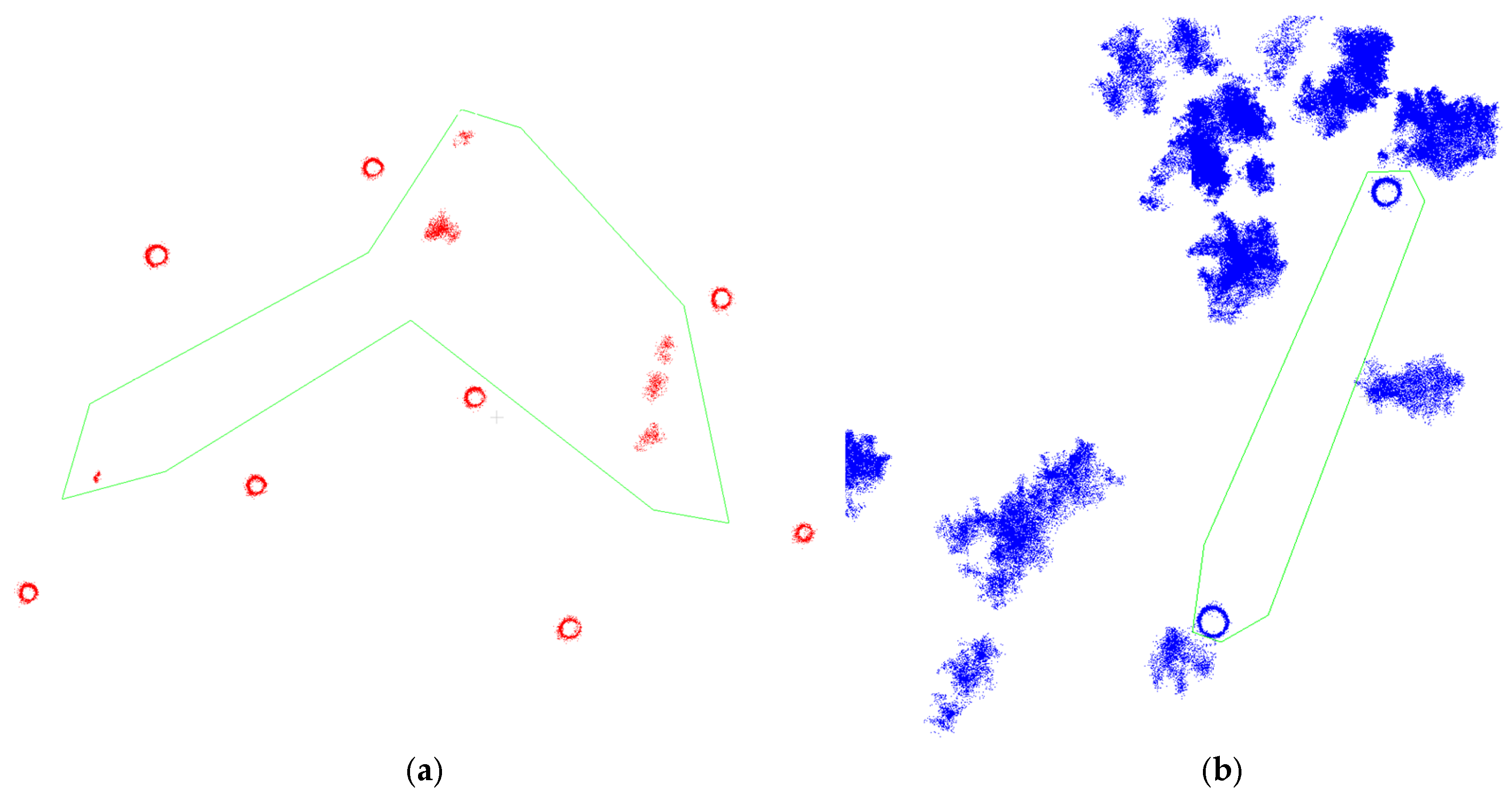
Figure 25.
An illustration of the manual inspection step, where the green polygon indicates the manual selected region: (a) outlier point removal, and (b) manual cropping identified missing stems.
Figure 25.
An illustration of the manual inspection step, where the green polygon indicates the manual selected region: (a) outlier point removal, and (b) manual cropping identified missing stems.
Figure 26.
Final check with the normalized height interval: (a) combined refined stems with the identified missing stems (in blue), (b) stems filtered out during clustering step (in black), and (c) the final reference stem map.
Figure 26.
Final check with the normalized height interval: (a) combined refined stems with the identified missing stems (in blue), (b) stems filtered out during clustering step (in black), and (c) the final reference stem map.
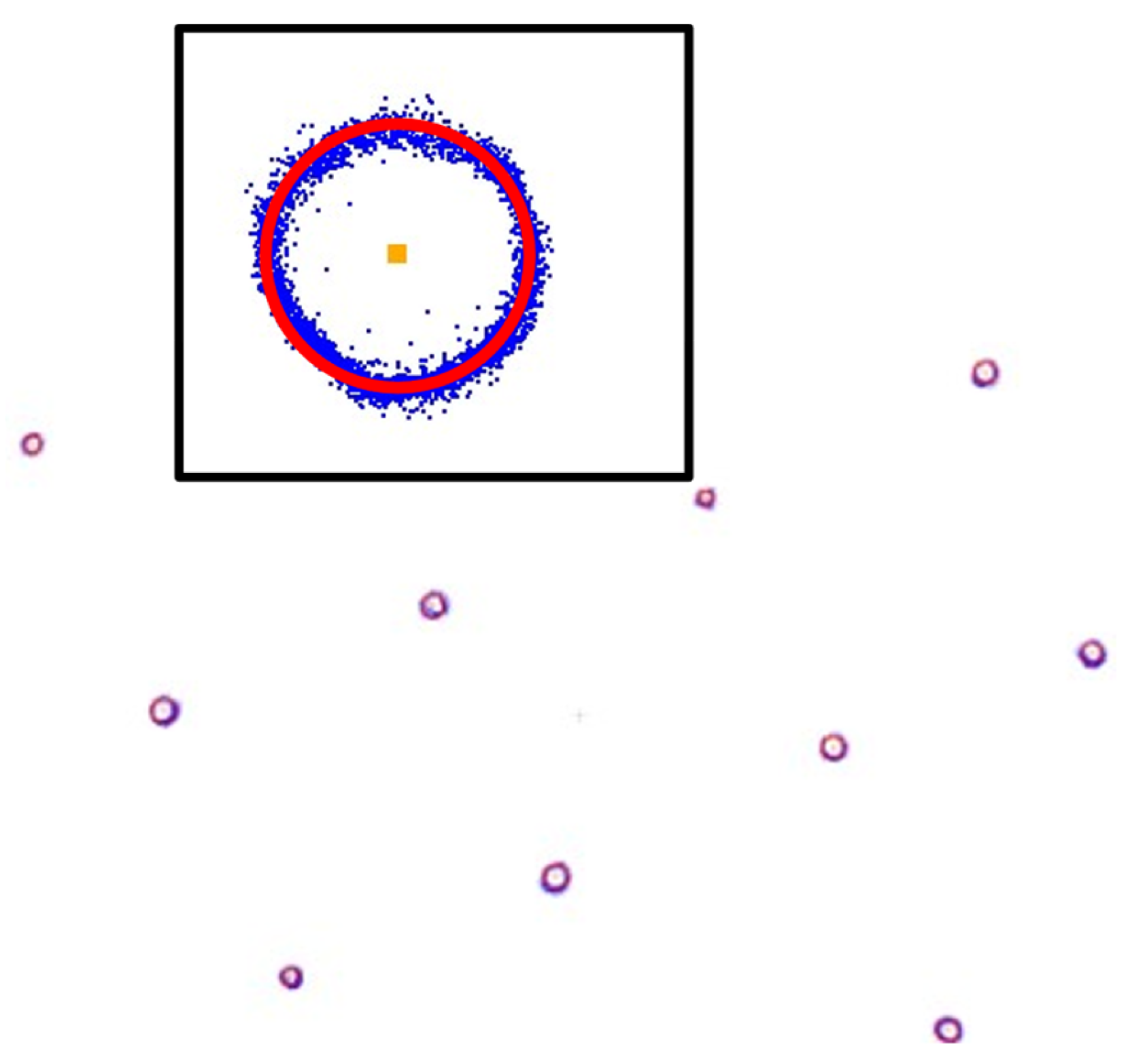
Figure 27.
Reference stem locations (in orange) with fitted circle (in red).
Figure 27.
Reference stem locations (in orange) with fitted circle (in red).
Figure 28.
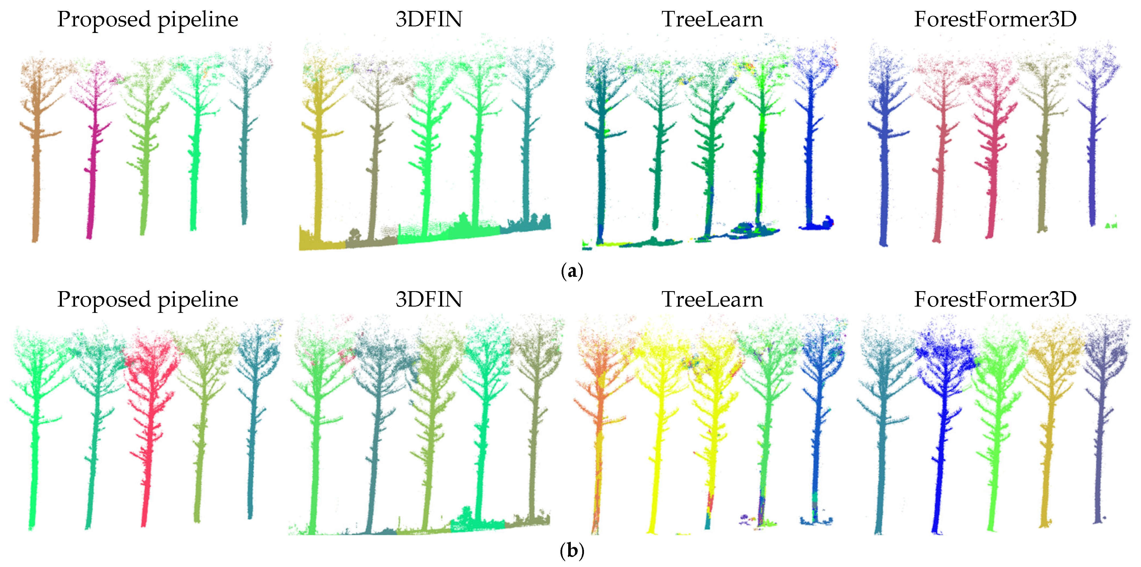
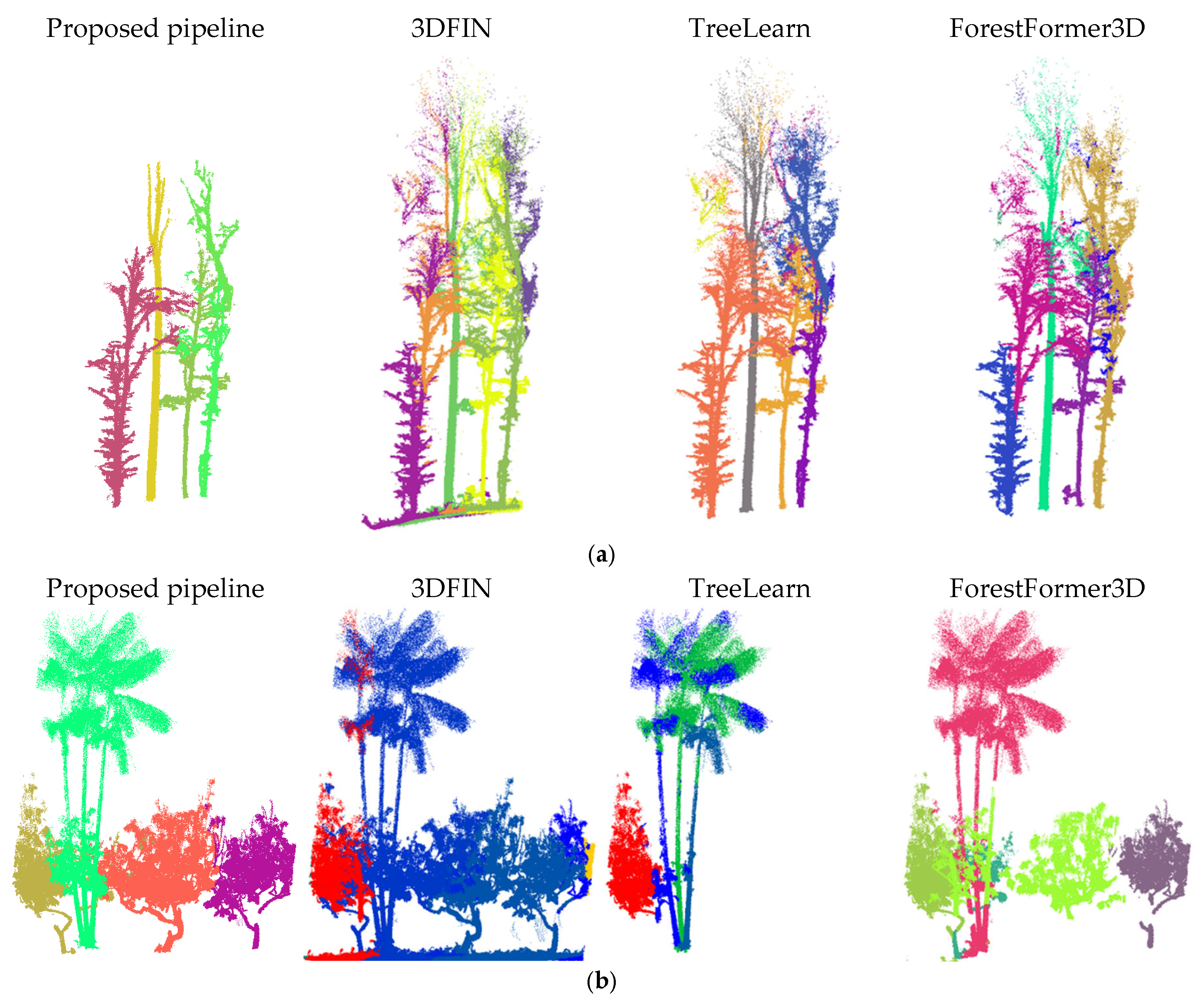
Qualitative comparison of tree- segmentation results colored by tree: (a) Whitehall–BackPack dataset, and (b) Whitehall–ATV dataset. TreeLearn shows visible over-segmentation, whereas the proposed pipeline maintains meaningful tree instances across both platforms.
Figure 28.
Qualitative comparison of tree- segmentation results colored by tree: (a) Whitehall–BackPack dataset, and (b) Whitehall–ATV dataset. TreeLearn shows visible over-segmentation, whereas the proposed pipeline maintains meaningful tree instances across both platforms.
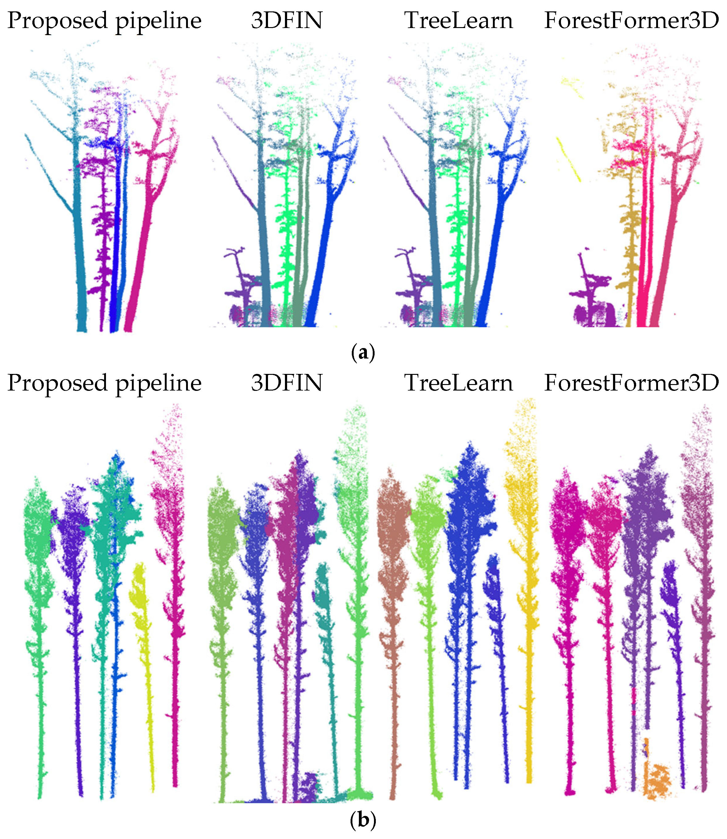
Figure 29.
Qualitative comparison of tree segmentation results colored by tree: (a) Martell–BackPack dataset, and (b) Martell–UAV dataset. The proposed pipeline and TreeLearn provide the clearest separation in the UAV case, while ForestFormer3D shows several missed or under-segmented trees.
Figure 29.
Qualitative comparison of tree segmentation results colored by tree: (a) Martell–BackPack dataset, and (b) Martell–UAV dataset. The proposed pipeline and TreeLearn provide the clearest separation in the UAV case, while ForestFormer3D shows several missed or under-segmented trees.
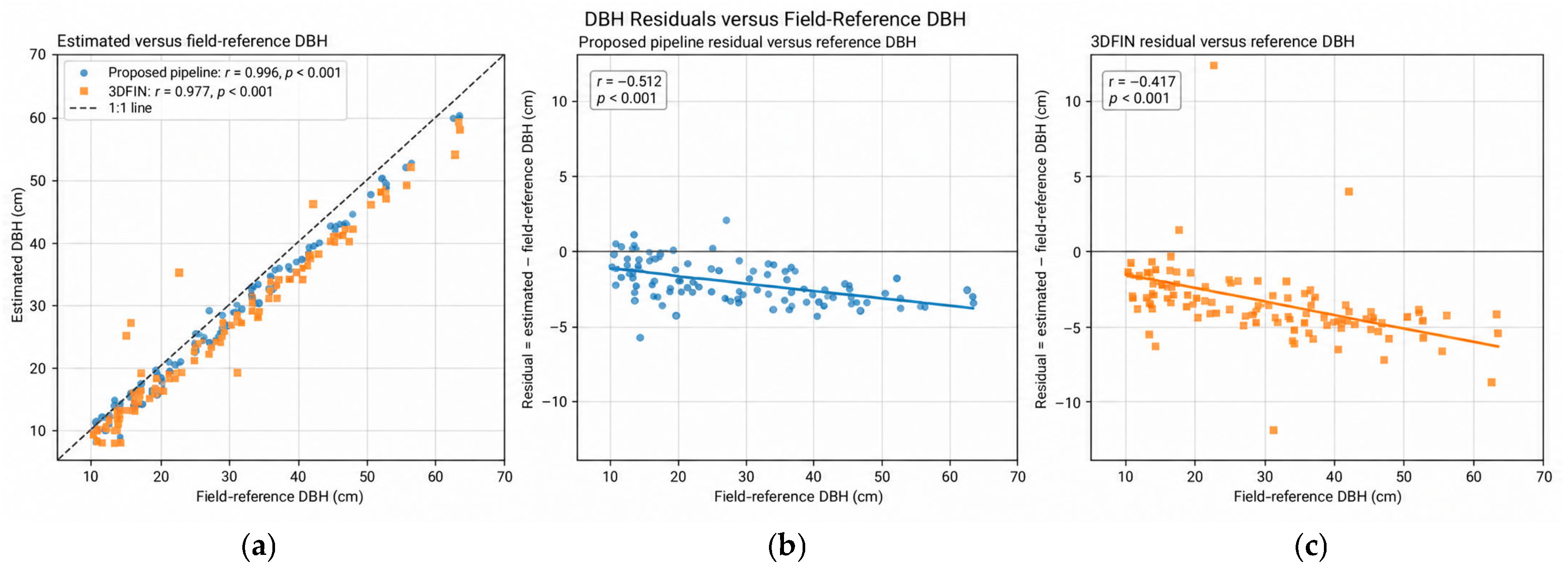
Figure 30.
DBH evaluation for the Martell–BackPack dataset: (a) comparison of estimated and field-reference DBH values for the proposed pipeline and 3DFIN; (b) DBH residuals as a function of field-reference DBH for the proposed pipeline; and (c) DBH residuals as a function of field-reference DBH for 3DFIN.
Figure 30.
DBH evaluation for the Martell–BackPack dataset: (a) comparison of estimated and field-reference DBH values for the proposed pipeline and 3DFIN; (b) DBH residuals as a function of field-reference DBH for the proposed pipeline; and (c) DBH residuals as a function of field-reference DBH for 3DFIN.
Figure 31.
Representative stem cross-sections and fitted circles for DBH estimation in the Martell–BackPack dataset: (a) a regular stem cross-section with the fitted circle and (b) a multi-stem cross-section illustrating a more challenging circle fitting condition.
Figure 31.
Representative stem cross-sections and fitted circles for DBH estimation in the Martell–BackPack dataset: (a) a regular stem cross-section with the fitted circle and (b) a multi-stem cross-section illustrating a more challenging circle fitting condition.
Figure 32.
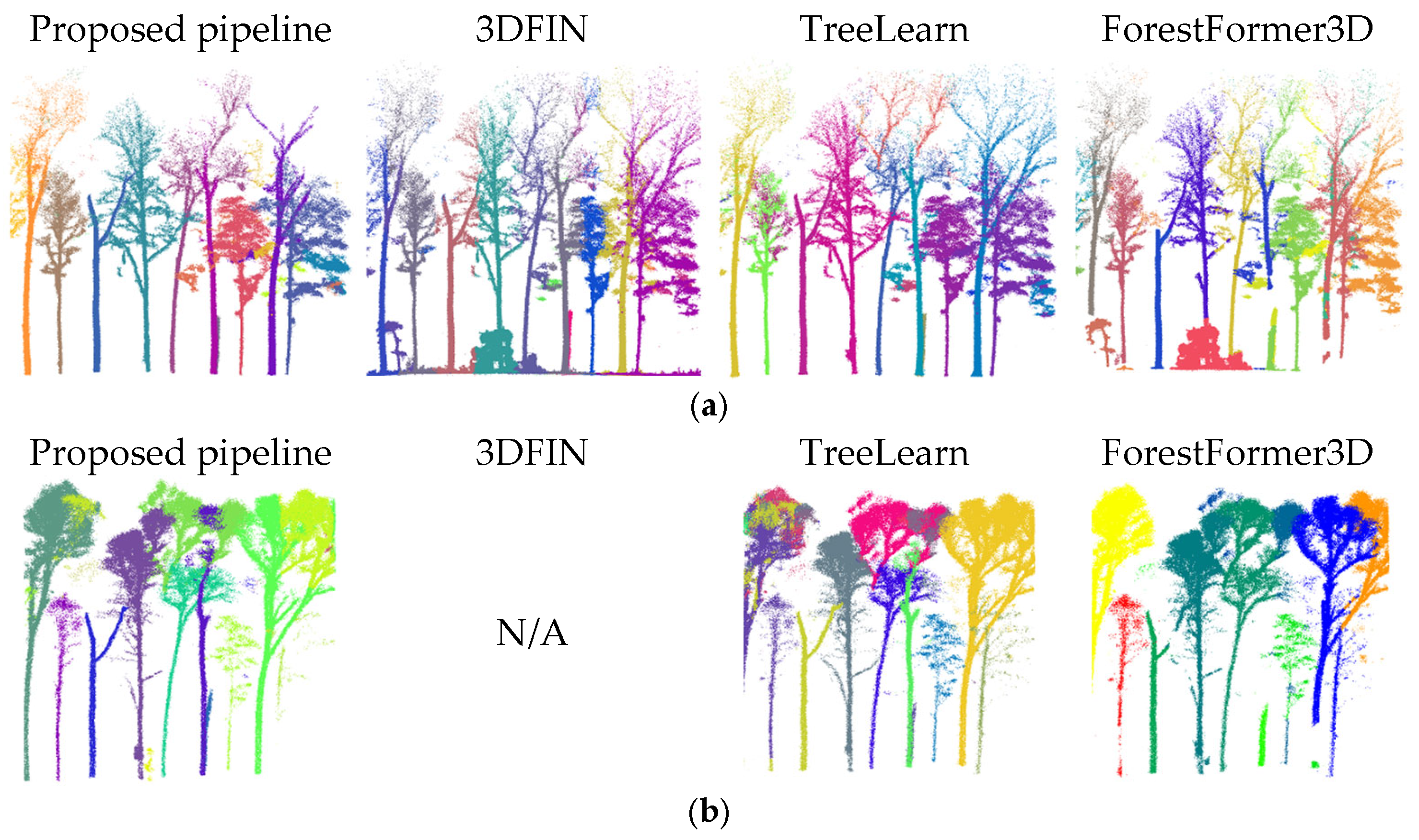
Qualitative comparison of tree segmentation results colored by tree: (a) Michigan–BackPack dataset, and (b) NIBIO–Handheld dataset. Sparse single-pass coverage affects all methods for the Michigan dataset, whereas the proposed pipeline provides more complete tree separation in the denser NIBIO dataset.
Figure 32.
Qualitative comparison of tree segmentation results colored by tree: (a) Michigan–BackPack dataset, and (b) NIBIO–Handheld dataset. Sparse single-pass coverage affects all methods for the Michigan dataset, whereas the proposed pipeline provides more complete tree separation in the denser NIBIO dataset.
Figure 33.
Qualitative comparison of tree segmentation results colored by tree: (a) SEPAC–BackPack dataset, and (b) Brazil–BackPack dataset. The proposed pipeline maintains clearer tree separation under dense understory and preserves smaller trees in the tropical dataset.
Figure 33.
Qualitative comparison of tree segmentation results colored by tree: (a) SEPAC–BackPack dataset, and (b) Brazil–BackPack dataset. The proposed pipeline maintains clearer tree separation under dense understory and preserves smaller trees in the tropical dataset.
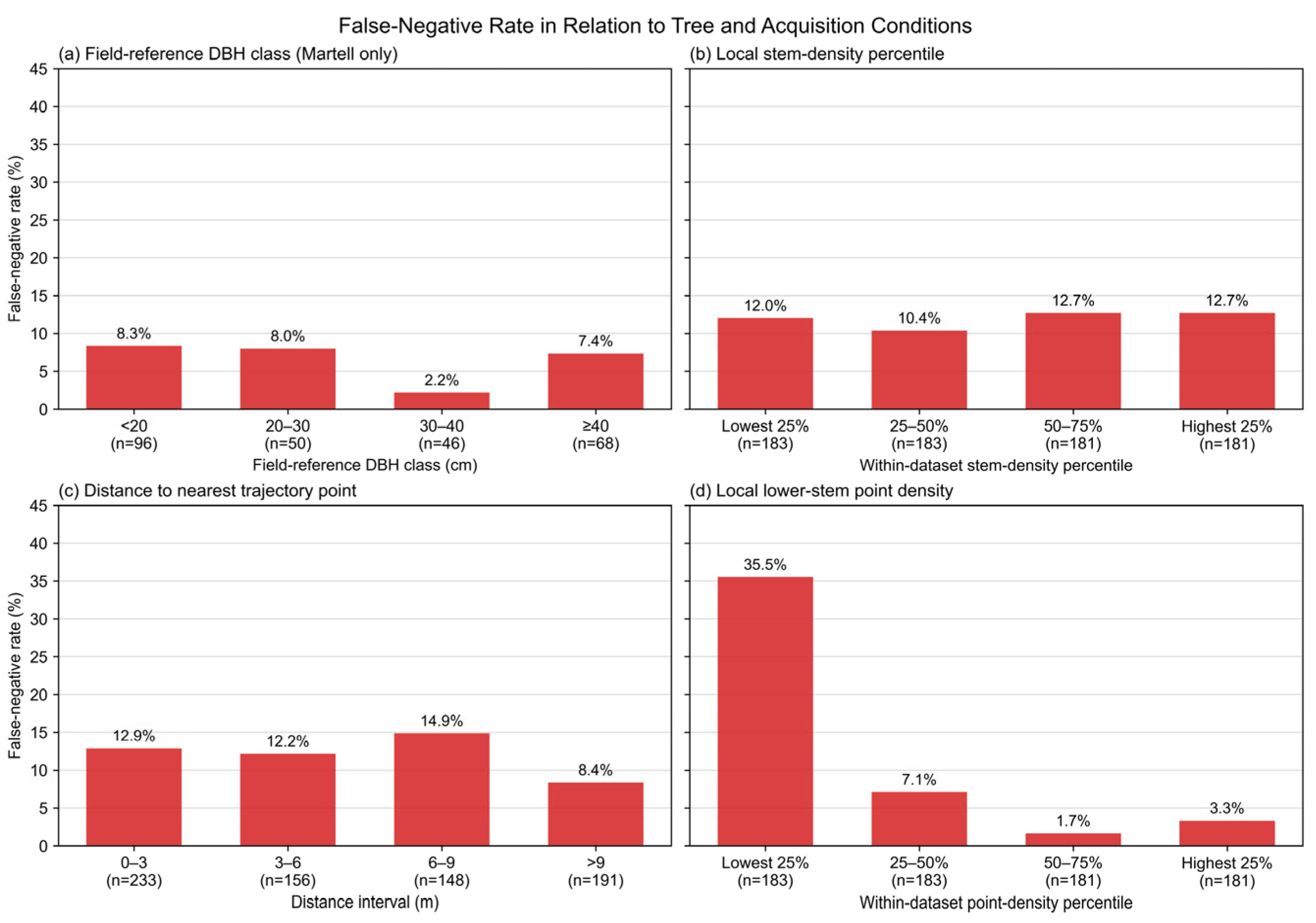
Figure 34.
The false negative rate according to (a) field-reference DBH class for the Martell datasets, (b) within-dataset local stem density percentile, (c) distance to the nearest trajectory point, and (d) within-dataset local lower-stem point density percentile.
Figure 34.
The false negative rate according to (a) field-reference DBH class for the Martell datasets, (b) within-dataset local stem density percentile, (c) distance to the nearest trajectory point, and (d) within-dataset local lower-stem point density percentile.
Figure 35.
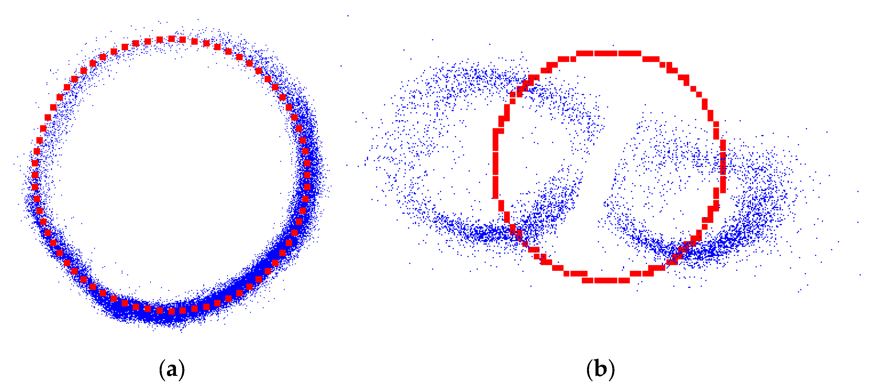
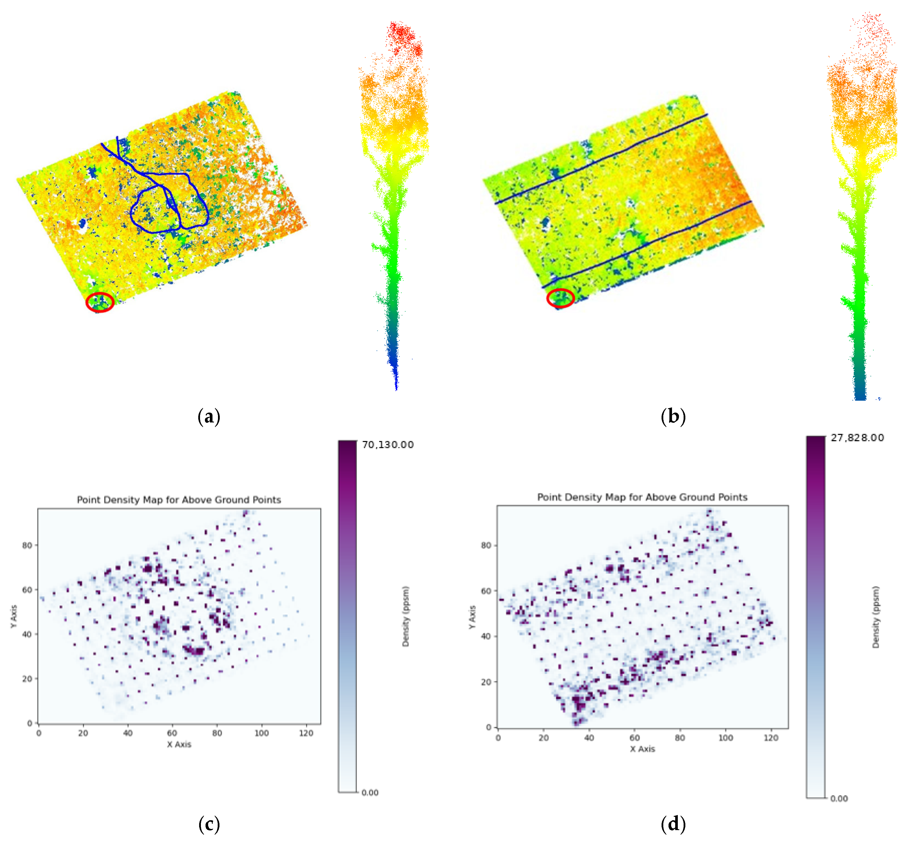
Illustration of trajectory pattern with sample border tree highlighted in red and point density maps for (a,c) Whitehall–BackPack dataset and (b,d) Whitehall–ATV dataset.
Figure 35.
Illustration of trajectory pattern with sample border tree highlighted in red and point density maps for (a,c) Whitehall–BackPack dataset and (b,d) Whitehall–ATV dataset.
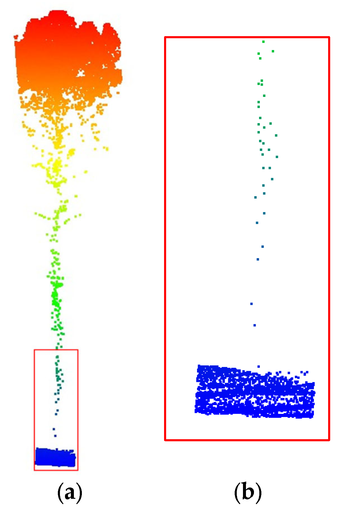
Figure 36.
An example of lower-stem discontinuity in the Martell–UAV point cloud colored by height: (a) the complete tree point cloud, and (b) a zoomed-in view of the lower stem highlighting gaps in stem observations caused by canopy occlusion.
Figure 36.
An example of lower-stem discontinuity in the Martell–UAV point cloud colored by height: (a) the complete tree point cloud, and (b) a zoomed-in view of the lower stem highlighting gaps in stem observations caused by canopy occlusion.
Figure 37.
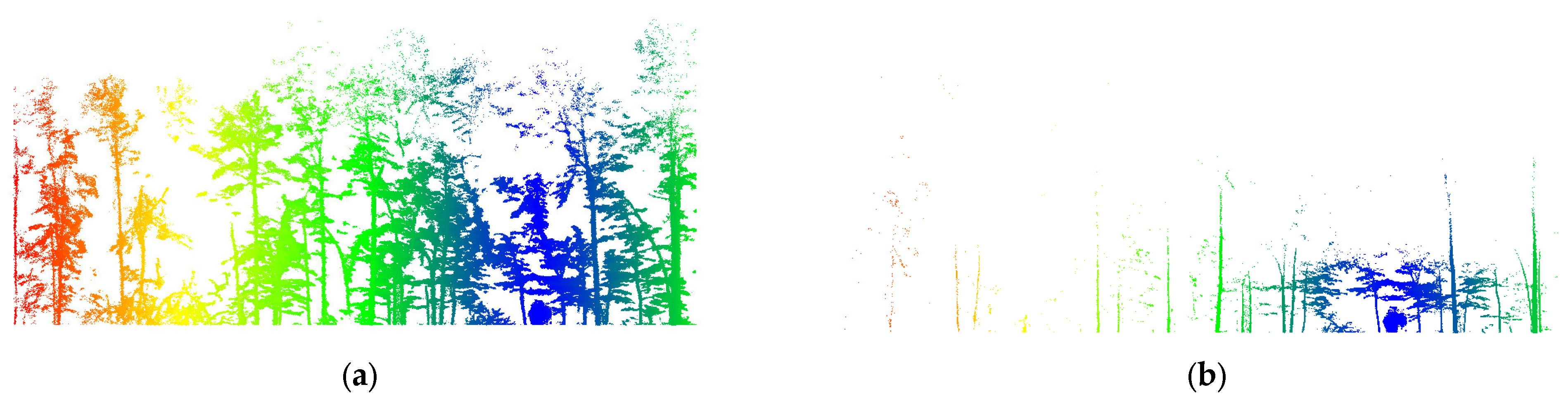
Illustration of intensity filtering effect on trees far from trajectory: (a) normalized height point cloud colored by distance from trajectory and (b) point cloud after intensity filtering.
Figure 37.
Illustration of intensity filtering effect on trees far from trajectory: (a) normalized height point cloud colored by distance from trajectory and (b) point cloud after intensity filtering.
Table 1.
LiDAR dataset description.
Table 1.
LiDAR dataset description.
| Site | Platform | Environment | Collection Date | Number of Total Points |
|---|
| Whitehall | BackPack-Knap-XP1 | Plantation forest | 11 May 2025 | 86,246,755 |
ATV-
Knap-XP1 | 15 May 2025 | 19,834,229 |
| Martell 4D | UAV-Altax | Natural forest | 27 February 2025 | 15,501,291 |
| BackPack-E2HDL32E | 4 December 2024 | 203,423,274 |
| Michigan | BackPack-Knap-XP1 | 28 May 2025 | 58,805,447 |
| NIBIO | Handheld-Horizon RT | Dense boreal forest | N/A | 40,525,844 |
| SEPAC | BackPack-E2HDL32E | Natural forest | 19 November 2024 | 82,282,252 |
| Brazil | Tropical forest | 5 November 2023 | 37,036,938 |
Table 2.
Implementation settings adopted for the comparative evaluation of the benchmark methods.
Table 2.
Implementation settings adopted for the comparative evaluation of the benchmark methods.
| Method | Software and Model Used | Main Configuration | Dataset Adjustment |
|---|
| 3DFIN | Official 3DFIN software, version 0.6.0 | Official default configuration, including stem detection, section extraction, and circle fitting settings | The same configuration was applied to all supported datasets |
| TreeLearn | Official TreeLearn implementation using the provided model_weights_20241213.pth pretrained model | Tree confidence threshold: 0.5; verticality threshold: 0.6; maximum offset: 4 m; minimum cluster size: 50; HDBSCAN grouping | The same pretrained model and inference settings were applied to all datasets |
| ForestFormer3D | Official ForestFormer3D implementation using the provided epoch_3000_fix.pth pretrained model | Cylinder radius: 16 m; voxel size: 0.20 m; number of queries: 300; score threshold: 0.4; official two-pass inference procedure | The same pretrained model and inference settings were applied to all datasets |
Table 3.
Point counts and total processing time for the proposed pipeline and benchmark methods.
Table 3.
Point counts and total processing time for the proposed pipeline and benchmark methods.
| Dataset | Number of Points | Processing Time in Minutes |
|---|
| Proposed Pipeline | 3DFIN | TreeLearn | ForestFormer3D |
|---|
| Whitehall–BackPack | 86,246,755 | 30 | 12 | 19 | 48 |
| Whitehall–ATV | 19,834,229 | 10 | 7 | 30 | 67 |
| Martell–UAV | 15,501,291 | 8 | - | 11 | 10 |
| Martell–BackPack | 203,423,274 | 102 | 14 | 24 | 116 |
| Michigan | 58,805,447 | 21 | 24 | 19 | 35 |
| NIBIO | 40,525,844 | 9 | 14 | 11 | 24 |
| SEPAC | 82,282,252 | 28 | 20 | 31 | 48 |
| Brazil | 37,036,938 | 12 | 14 | 12 | 41 |
Table 4.
A summary of tree detection performance and available biometric evaluation results for the proposed pipeline and benchmark methods across the evaluated datasets.
Table 4.
A summary of tree detection performance and available biometric evaluation results for the proposed pipeline and benchmark methods across the evaluated datasets.
| Approach | Site | Dataset | Reference Type | No. of Reference Trees | Precision | Recall | F1-Score | DBH RMSE | Basal Area Error |
|---|
| Proposed pipeline | Whitehall | Whitehall–BackPack | Point cloud-based reference measurements | 80 | 97.53% | 98.75% | 98.15% | - | - |
| 3DFIN | 95.18% | 98.75% | 96.93% | - | - |
| TreeLearn | 13.47% | 88.75% | 23.39% | - | - |
| ForestFormer3D | 88.88% | 100.00% | 94.11% | - | - |
| Proposed pipeline | Whitehall–ATV | 100.00% | 100.00% | 100.00% | - | - |
| 3DFIN | 93.67% | 92.5% | 93.08% | - | - |
| TreeLearn | 22.26% | 73.75% | 34.20% | - | - |
| ForestFormer3D | 76.92% | 100.00% | 86.95% | - | - |
| Proposed pipeline | Martell | Martell–BP | Field-based reference measurements | 164 | 97.55% | 96.95% | 97.25% | 2.5 cm | −1.88% |
| 3DFIN | 86.66% | 95.12% | 90.69% | 4 cm | −3.67% |
| TreeLearn | 87.15% | 95.12% | 90.96% | - | - |
| ForestFormer3D | 34.33% | 62.80% | 44.39% | - | - |
| Proposed pipeline | Martell–UAV | 92.72% | 85.37% | 88.89% | - | - |
| 3DFIN | - | - | - | - | - |
| TreeLearn | 99.27% | 85.37% | 91.80% | - | - |
| ForestFormer3D | 90.60% | 64.63% | 75.44% | - | - |
| Proposed pipeline | Michigan | Michigan–BackPack | Point cloud-based reference measurements | 182 | 91.21% | 74.17% | 81.82% | - | - |
| 3DFIN | 78.43% | 87.91% | 82.90% | - | - |
| TreeLearn | 74.46% | 76.92% | 75.67% | - | - |
| ForestFormer3D | 50.68% | 60.98% | 55.36% | - | - |
| Proposed pipeline | NIBIO | NIBIO–Handheld | 72 | 90.14% | 88.88% | 89.51% | - | - |
| 3DFIN | 100.00% | 66.66% | 80.00% | - | - |
| TreeLearn | 95.91% | 65.27% | 77.68% | - | - |
| ForestFormer3D | 90.47% | 79.16% | 84.44% | - | - |
| Proposed pipeline | SEPAC | SEPAC–BackPack | 58 | 86.44% | 87.93% | 87.18% | - | - |
| 3DFIN | 56.52% | 89.66% | 69.33% | - | - |
| TreeLearn | 80.32% | 84.48% | 82.35% | - | - |
| ForestFormer3D | 50.00% | 86.20% | 63.29% | - | - |
| Proposed pipeline | Brazil | Brazil–BackPack | 122 | 87.20% | 89.34% | 88.26% | - | - |
| 3DFIN | 82.53% | 42.62% | 56.21% | - | - |
| TreeLearn | 52.63% | 32.78% | 40.40% | - | - |
| ForestFormer3D | 70.00% | 40.16% | 51.04% | - | - |
Table 5.
Comparison of tree detection performance for the Whitehall–BackPack and ATV datasets.
Table 5.
Comparison of tree detection performance for the Whitehall–BackPack and ATV datasets.
| Approach | Site | Dataset | Reference Type | No. of Reference Trees | TP | FP | FN | Precision | Recall | F1-Score |
|---|
| Proposed pipeline | Whitehall | Whitehall–BackPack | Point cloud-based reference measurements | 80 | 79 | 2 | 1 | 97.53% | 98.75% | 98.15% |
| 3DFIN | 79 | 4 | 1 | 95.18% | 98.75% | 96.93% |
| TreeLearn | 71 | 456 | 9 | 13.47% | 88.75% | 23.39% |
| ForestFormer3D | 80 | 10 | 0 | 88.88% | 100.00% | 94.11% |
| Proposed pipeline | Whitehall–ATV | 80 | 0 | 0 | 100.00% | 100.00% | 100.00% |
| 3DFIN | 74 | 5 | 6 | 93.67% | 92.5% | 93.08% |
| TreeLearn | 59 | 206 | 21 | 22.26% | 73.75% | 34.20% |
| ForestFormer3D | 80 | 24 | 0 | 76.92% | 100.00% | 86.95% |
Table 6.
Statistics of tree detection results from different approaches for Martell–BackPack and UAV datasets.
Table 6.
Statistics of tree detection results from different approaches for Martell–BackPack and UAV datasets.
| Approach | Site | Dataset | Reference Type | No. of Reference Trees | TP | FP | FN | Precision | Recall | F1-Score |
|---|
| Proposed pipeline | Martell 4D | Martell–BackPack | Field-based reference measurements | 164 | 159 | 4 | 5 | 97.55% | 96.95% | 97.25% |
| 3DFIN | 156 | 24 | 8 | 86.66% | 95.12% | 90.69% |
| TreeLearn | 156 | 23 | 8 | 87.15% | 95.12% | 90.96% |
| ForestFormer3D | 103 | 197 | 61 | 34.33% | 62.80% | 44.39% |
| Proposed pipeline | Martell–UAV | 140 | 11 | 24 | 92.72% | 85.37% | 88.89% |
| TreeLearn | 140 | 1 | 24 | 99.27% | 85.37% | 91.80% |
| ForestFormer3D | 106 | 11 | 58 | 90.60% | 64.63% | 75.44% |
Table 7.
Statistical comparison of estimated and field-measured DBH values for correctly detected trees in the Martell–BackPack dataset.
Table 7.
Statistical comparison of estimated and field-measured DBH values for correctly detected trees in the Martell–BackPack dataset.
| Approach | No. of Trees | Min (cm) | Max (cm) | Mean (cm) | Median (cm) | Std (cm) | RMSE (cm) | r | p-Value |
|---|
| Proposed pipeline | 156 | 0.0 | −5.7 | −2.1 | −2.3 | 1.2 | 2.5 | 0.996 | <0.001 |
| 3DFIN | 0.4 | 9.9 | 3.4 | 3.7 | 1.6 | 4.0 | 0.977 | <0.001 |
Table 8.
Inventory-level basal area comparison for the Martell–BackPack dataset.
Table 8.
Inventory-level basal area comparison for the Martell–BackPack dataset.
| Approach | Basal Area (m2) | Difference (m2) | Relative Difference |
|---|
| Field reference | 11.17 | - | - |
| Proposed pipeline | 10.96 | −0.21 | −1.88% |
| 3DFIN | 10.76 | −0.41 | −3.67% |
Table 9.
Tree detection performance for Michigan–BackPack and NIBIO–Handheld datasets.
Table 9.
Tree detection performance for Michigan–BackPack and NIBIO–Handheld datasets.
| Approach | Site | Dataset | Reference Type | No. of Reference Trees | TP | FP | FN | Precision | Recall | F1-Score |
|---|
| Proposed pipeline | Michigan | Michigan–BackPack | Point cloud-based reference measurements | 182 | 135 | 13 | 47 | 91.21% | 74.17% | 81.82% |
| 3DFIN | 160 | 44 | 22 | 78.43% | 87.91% | 82.90% |
| TreeLearn | 140 | 48 | 42 | 74.46% | 76.92% | 75.67% |
| ForestFormer3D | 111 | 108 | 71 | 50.68% | 60.98% | 55.36% |
| Proposed pipeline | NIBIO | NIBIO–Handheld | 72 | 64 | 7 | 8 | 90.14% | 88.88% | 89.51% |
| 3DFIN | 48 | 0 | 24 | 100.00% | 66.66% | 80.00% |
| TreeLearn | 47 | 2 | 25 | 95.91% | 65.27% | 77.68% |
| ForestFormer3D | 57 | 6 | 15 | 90.47% | 79.16% | 84.44% |
Table 10.
Tree detection performance of proposed pipeline and benchmark methods on SEPAC–BackPack and Brazil–BackPack datasets.
Table 10.
Tree detection performance of proposed pipeline and benchmark methods on SEPAC–BackPack and Brazil–BackPack datasets.
| Approach | Site | Dataset | Reference Type | No. of Reference Trees | TP | FP | FN | Precision | Recall | F1-Score |
|---|
| Proposed pipeline | SEPAC | SEPAC–BackPack | Point cloud-based reference measurements | 58 | 51 | 8 | 7 | 86.44% | 87.93% | 87.18% |
| 3DFIN | 52 | 40 | 6 | 56.52% | 89.66% | 69.33% |
| TreeLearn | 49 | 12 | 9 | 80.32% | 84.48% | 82.35% |
| ForestFormer3D | 50 | 50 | 8 | 50.00% | 86.20% | 63.29% |
| Proposed pipeline | Brazil | Brazil–BackPack | 122 | 109 | 16 | 13 | 87.20% | 89.34% | 88.26% |
| 3DFIN | 52 | 11 | 70 | 82.53% | 42.62% | 56.21% |
| TreeLearn | 40 | 36 | 82 | 52.63% | 32.78% | 40.40% |
| ForestFormer3D | 49 | 21 | 73 | 70.00% | 40.16% | 51.04% |
Table 11.
Ablation results for optional 3D U-Net understory–removal module.
Table 11.
Ablation results for optional 3D U-Net understory–removal module.
| Dataset | Understory Removal | TP | FP | FN | Precision | Recall | F1-Score |
|---|
| Martell–BackPack | Enabled | 159 | 4 | 5 | 97.55% | 96.95% | 97.25% |
| Disabled | 146 | 77 | 18 | 65.47% | 89.02% | 75.45% |
| Brazil–BackPack | Disabled | 109 | 16 | 13 | 87.20% | 89.34% | 88.26% |
| Enabled | 15 | 22 | 107 | 40.54% | 12.30% | 18.87% |
Table 12.
Tile size and overlap buffer sensitivity analysis.
Table 12.
Tile size and overlap buffer sensitivity analysis.
| Tile Size (m) | Buffer (m) | Number of Tiles | Processed Point Records | Processing Time (min) | Detected Trees in Common 30 × 30 m Area |
|---|
| 30 | 5.0 | 8 | 199,038,310 | 51.30 | 59 |
| 50 | 2.5 | 3 | 112,686,528 | 26.07 | 59 |
| 50 | 5.0 | 3 | 134,895,822 | 32.51 | 59 |
| 50 | 7.5 | 3 | 156,440,939 | 39.71 | 59 |
| 70 | 5.0 | 1 | 118,814,465 | 36.80 | 59 |