Article

A Unified Framework for Individual Tree Segmentation and Forest Biometrics Derivation from LiDAR Point Clouds Captured by Different Platforms in Diverse Forest Environments

1
Lyles School of Civil and Construction Engineering, Purdue University, West Lafayette, IN 47907, USA
2
Department of Forestry and Natural Resources, Purdue University, West Lafayette, IN 47907, USA
*
Author to whom correspondence should be addressed.
Remote Sens. 2026, 18(17), 3059; https://doi.org/10.3390/rs18173059
Submission received: 11 June 2026 / Revised: 11 August 2026 / Accepted: 3 September 2026 / Published: 7 September 2026

Highlights

What are the main findings?
  • A LiDAR workflow using parameter configurations fixed within each acquisition modality was developed for individual tree segmentation and the derivation of forest biometrics, including tree location and diameter at breast height.
  • The framework achieved consistent tree detection accuracy across eight heterogeneous forest datasets and improved DBH estimation compared with the benchmark method capable of deriving DBH.
What are the implication of the main finding?
  • The proposed workflow provides a scalable solution for LiDAR-based Forest inventory without site-specific parameter tuning within each acquisition modality or model retraining.
  • The confidence-guided quality control strategy enables reliable individual tree and stand-level biometrics extraction across diverse forest structures and acquisition platforms.

Abstract

Light Detection and Ranging (LiDAR)-based forest inventory increasingly relies on diverse platforms, ranging from proximal systems including BackPack, All-Terrain Vehicle (ATV), and terrestrial laser scanning (TLS) to near-proximal systems such as uncrewed aerial vehicles (UAVs). However, differences in point density, viewing geometry, and occlusions among these acquisition systems pose challenges for processing heterogeneous LiDAR datasets using a common workflow. Traditional geometric approaches often rely on parameter tuning. On the other hand, deep learning (DL) approaches can be constrained by domain shift when applied to different sensors or forest environments. This study proposes a forest inventory pipeline for individual tree segmentation and the derivation of key forest biometrics including tree location and diameter at breast height (DBH) across heterogeneous LiDAR datasets. The pipeline uses a confidence-guided, multi-stage quality control framework that evaluates agreement between complementary tree location estimates to reduce common segmentation errors. In addition, a semi-automated procedure is developed to generate reference data for datasets lacking field measurements. The proposed workflow was evaluated using eight diverse datasets representing different platforms, sensors, acquisition patterns, and forest environments and was compared with 3DFIN, TreeLearn, and ForestFormer3D. Field reference measurements were available for a natural forest site, while the remaining datasets were evaluated using semi-automatically generated and manually refined reference data. The proposed tree detection pipeline achieved Precision ranging from 86.44% to 100%, Recall from 74.17% to 100%, and F1-scores from 81.82% to 100% across the evaluated datasets. For the Martell–BackPack dataset with independent field reference measurements, Precision, Recall, and F1-score were 97.55%, 96.95%, and 97.25%, respectively. For correctly detected trees by the proposed approach in the natural forest dataset with field measurements, DBH estimates achieved an RMSE of 2.5 cm with the total basal area underestimated by 1.88%, compared with DBH RMSE and reduction in basal area of 4.0 cm and 3.67%, respectively, for 3DFIN. Although the proposed pipeline did not achieve the highest performance in every test case, it maintained strong and generally consistent tree detection performance for the evaluated datasets. The main limitation of the proposed pipeline is its dependence on sufficient lower-stem visibility, which reduced tree detection accuracy in sparsely sampled areas. The proposed framework provides a practical workflow for LiDAR-based individual tree segmentation and DBH estimation using a fixed parameter configuration for all datasets captured by a given acquisition system.

1. Introduction

Fine-resolution forest inventory, which quantifies individual tree metrics such as location, height, and diameter at breast height (DBH), underpins sustainable forest management, carbon accounting, and climate change mitigation [1]. These metrics are essential for estimating timber volume, assessing forest health, monitoring growth and mortality, and tracking how much carbon is stored in above-ground biomass. However, conventional plot-based field inventories are labor-intensive, costly, and difficult to employ, especially in remote or densely vegetated forests. As a result, traditional field methods struggle to meet the spatial and temporal demands of modern Precision forestry [2].
Light Detection and Ranging (LiDAR) has transformed forest inventory practices by enabling rapid, three-dimensional characterization of forest structure [3]. LiDAR data are now routinely acquired from traditional airborne systems, as well as from near-proximal platforms such as uncrewed aerial vehicles (UAVs) and proximal systems including terrestrial laser scanning (TLS) and terrestrial mobile mapping systems (MMSs), each with distinct point densities, occlusion patterns, and levels of detail [4]. This range of acquisition platforms has expanded forest inventory applications from large-area canopy assessment to detailed stem-level mapping. At the same time, it has introduced variation in point cloud structure and visibility, creating challenges for methods intended to operate consistently across several acquisition settings [5].
Near-proximal systems such as UAVs provide efficient coverage of large areas and are effective for capturing upper-canopy structure, including tree height and crown metrics [6]. However, their top–down perspective is affected by foliage occlusions, which can limit observations of the lower stem and forest floor and reduce the reliability of DBH estimation [2,7]. In contrast, proximal systems such as TLS and terrestrial MMS provide denser measurements of the forest floor and are commonly used for detailed stem mapping and DBH estimation [8]. However, proximal LiDAR systems mainly observe trees from below, which can limit the coverage of crowns and upper branches. Below-canopy mobile acquisitions may also produce uneven point densities and irregular sampling patterns. These differences between proximal and near-proximal point clouds make it difficult to process data captured by both acquisition modalities using the same workflow.
These platform-specific characteristics have directly influenced the design of individual tree segmentation (ITS) algorithms. Top–down approaches developed for aerial LiDAR commonly identify local maxima from canopy height models and delineate tree crowns using watershed or region-growing procedures [9]. Although these methods can perform well in relatively simple canopy conditions, they may miss subcanopy trees and under-segment neighboring crowns in mixed or structurally complex forests. Their performance can also be sensitive to parameter choices such as canopy-height-model smoothing level and window size [10,11].
Bottom–up approaches developed for proximal LiDAR typically identify stem candidates using horizontal projections, clustering, or cylinder fitting before applying region growing to recover the complete tree [12]. These approaches can provide accurate stem locations and DBH estimates when the lower stem is sufficiently observed. However, dense understory, low branches, closely spaced trees, and incomplete stem coverage can produce false stem detections and under- or over-segmentation. Their dependence on sufficiently covered stem structures also limits their direct application to top–down point clouds, where lower-stem coverage is often sparse [8,13].
More advanced geometric ITS approaches combine multiple processing stages to improve segmentation consistency and address common errors. For example, TLS2trees integrates semantic classification, graph construction, and post-processing refinement. Treegraph reconstructs tree architecture from point cloud data, whereas Treeiso separates individual trees using graph-based optimization [14,15,16]. Point2Tree provides a modular framework for tuning segmentation parameters for mobile laser scanning data, while 3DFIN is designed for TLS-based tree detection and estimation of structural attributes [17,18]. In our previous work, intensity filtering and DBSCAN clustering were used to segment individual trees in plantation and mixed-coniferous environments [19]. However, the approach was affected by under-segmentation when high stem density or irregular tree structures caused neighboring trees to be merged. Overall, the performance and transferability of geometric ITS approaches remain influenced by point density, viewing geometry, sensor noise, and the selected processing parameters.
Recently, deep learning (DL)-based ITS has emerged as a promising alternative. Architectures such as PointNet [20] demonstrated that neural networks can learn global and local geometric features directly from unordered 3D point clouds without explicit voxelization. Building on these advances, forestry-oriented models now target tree instance segmentation rather than only semantic segmentation. ForAINet [7] jointly performs semantic and instance segmentation of UAV point clouds and derives per-tree height, crown, and DBH estimates across diverse forest types. ForestFormer3D [21] extends this approach through a transformer-based, end-to-end framework designed to improve generalization across complex forest structures. TreeLearn [22] provides fully automatic tree instance segmentation from ground-based LiDAR. SegmentAnyTree [5] and Point2Tree [17] are examples of efforts to improve applicability across terrestrial and mobile datasets.
However, DL models still face substantial generalization challenges. Supervised models require large labeled point cloud datasets that are costly to produce, while existing multi-platform datasets cover only a limited range of sensors, platforms, and forest conditions [2,23]. Models trained on a specific acquisition configuration may experience considerable domain shift when applied to different platforms, sensors, point densities, or forest structures, particularly when transferring from dense terrestrial to sparse airborne data [24]. Consequently, fine-tuning is often required when transferring between coniferous and broadleaf stands, different point densities, or ground-based and aerial LiDAR datasets [5,22].
Overall, the existing literature on individual tree segmentation remains fragmented and platform-dependent. Geometric pipelines such as 3DFIN are typically designed for specific LiDAR platforms and forest types, and their accuracy depends strongly on point density and heuristic parameters. DL models such as ForAINet, TreeLearn, ForestFormer3D and SegmentAnyTree achieve strong results within their training domain, but they often require substantial retraining when the forest type or sensor changes. Moreover, when large forest point clouds are tiled for scalable processing, non-overlapping or independently processed tiles can split trees near tile boundaries, leading to incomplete segmentation or duplicated detections. These limitations prevent current methods from functioning as a general forest inventory workflow. The pipeline proposed in this study is designed to overcome these limitations by using a stem-guided localization and segmentation strategy, an overlapped tiling scheme that preserves complete trees across tile boundaries, and a multi-stage quality control module that together provide consistent tree segmentation and biometrics estimates across heterogeneous LiDAR datasets.
In this work, we propose a scalable pipeline for ITS and biometrics derivation designed to process heterogeneous LiDAR datasets using fixed parameter configurations within each acquisition system. The objectives of this study are to (1) develop a generalized workflow for individual tree segmentation and biometrics derivation from heterogeneous LiDAR datasets; (2) develop a confidence-guided multi-stage quality control framework that uses complementary stem location evidence to mitigate common segmentation errors, including false detections, under-segmentation, over-segmentation, multi-stem cases, and duplicated trees near tile boundaries; (3) develop a semi-automated reference-data generation procedure for quantitative accuracy assessment in datasets lacking field reference measurements; and (4) validate the developed workflow through comprehensive testing across diverse forest environments, platforms, sensors, and acquisition patterns, while benchmarking its performance against existing approaches.
The framework is motivated by the fact that initial stem clusters generated from forest point clouds are often affected by several factors, such as understory, low branches, closely spaced stems, and multi-stem trees. If these initial clusters are treated directly as final tree segments, they can result in under-segmentation, over-segmentation, and duplicated trees. Therefore, the proposed framework uses the agreement between complementary stem-location estimates not only to detect trees, but also to guide subsequent decisions on whether clusters should be retained, removed, split, refined, or cleaned near tile boundaries. The remainder of this paper is organized as follows: Section 2 describes the LiDAR systems, while Section 3 describes the study sites and datasets. Section 4 details the proposed forest inventory pipeline for processing heterogeneous LiDAR datasets. Section 5 presents experimental results and comprehensive analysis, including comparisons with benchmark algorithms. Section 6 provides the discussion, while the conclusions are presented in Section 7.

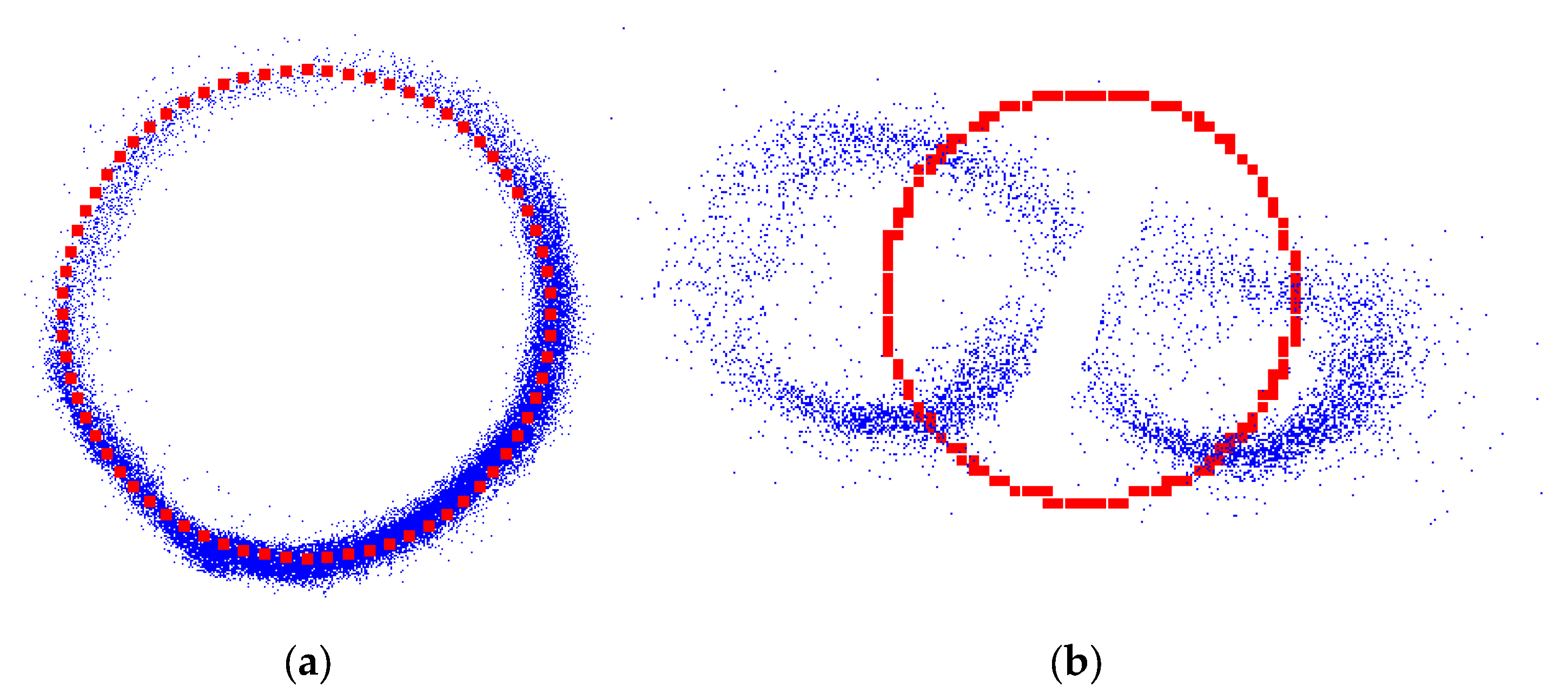
2. LiDAR Systems

This section describes the LiDAR systems and study sites used to evaluate the proposed pipeline. In total, eight datasets were collected across these platforms and sites. The datasets span both near-proximal and proximal acquisition systems, including UAV, BackPack, and vehicle-mounted LiDAR, and represent a range of forest structures and acquisition conditions.
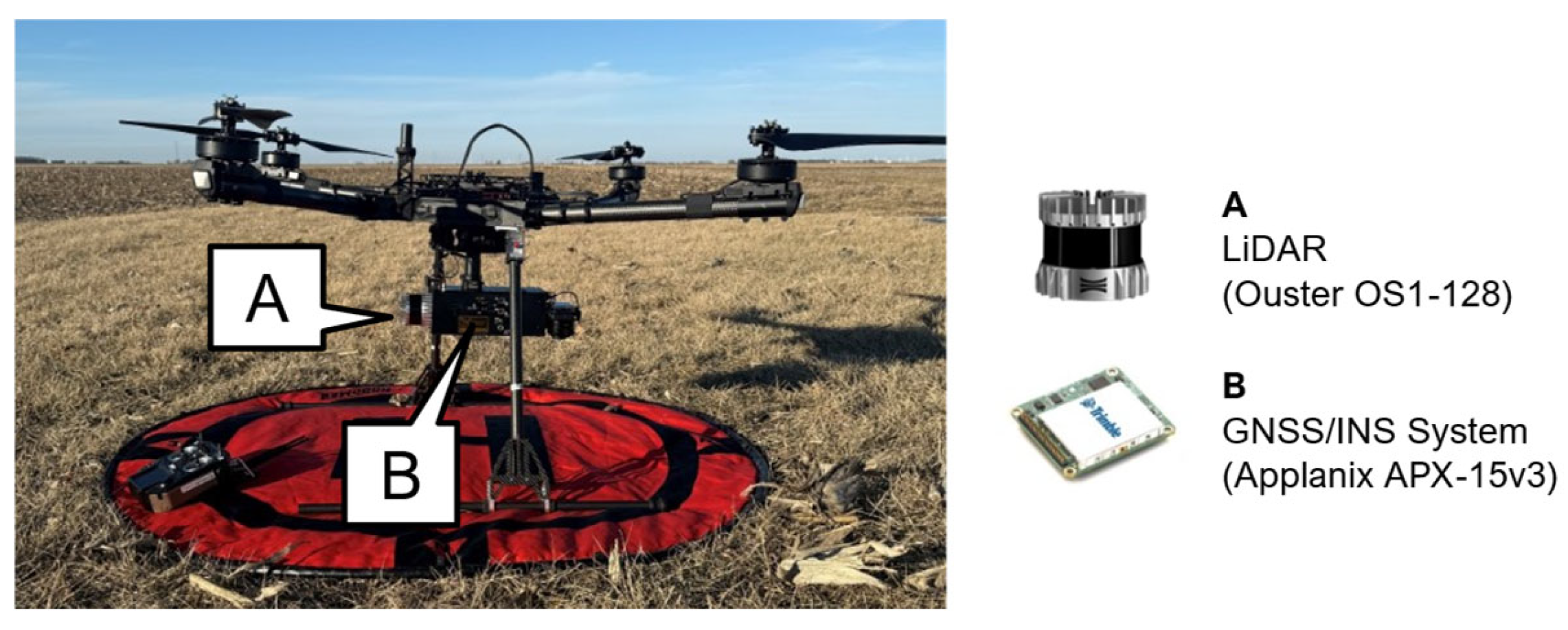
UAV LiDAR system: In this study, an in-house developed UAV LiDAR system is used for near-proximal data collection. The UAV shown in Figure 1 is equipped with an Ouster OS1-128 LiDAR sensor and an Applanix APX-15 v3 Global Navigation Satellite System/Inertial Navigation System (GNSS/INS) unit for georeferencing. The GNSS/INS records inertial measurement unit (IMU) data at 200 Hz [25]. After post-processing, the system achieves a positional accuracy of ±2 to ±5 cm under open-sky conditions, with angular accuracies of ±0.025° for roll and pitch and ±0.080° for heading, based on system provider specifications.
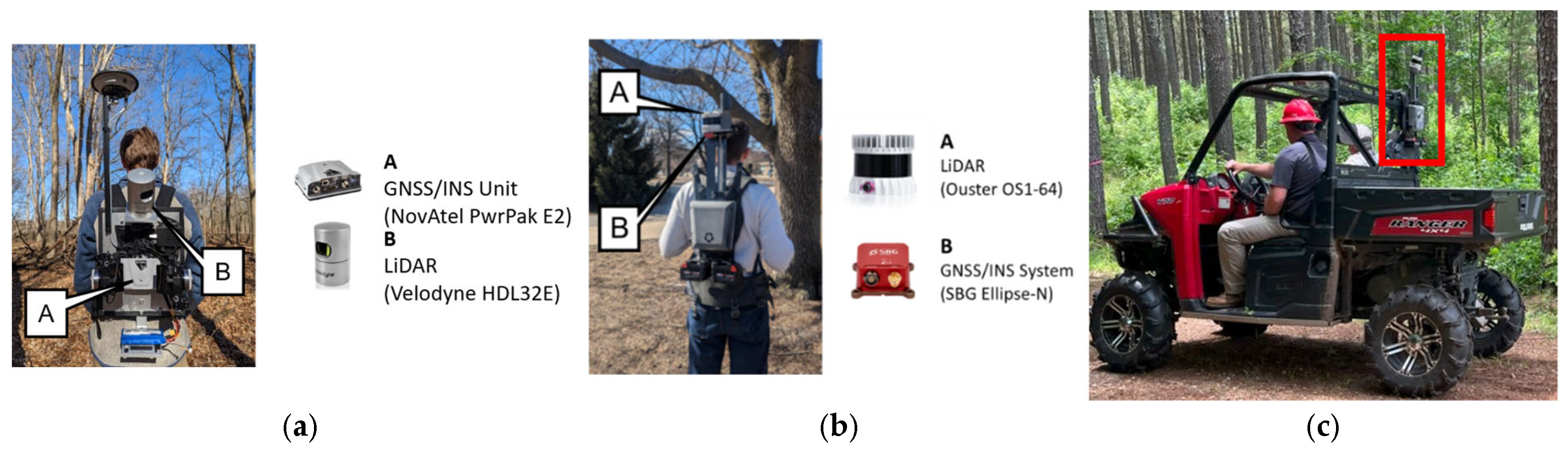
BackPack LiDAR Systems: Three in-house developed BackPack systems are used for proximal data collection. The first BackPack system, E2HDL32E shown in Figure 2a, consists of a Velodyne HDL-32E LiDAR sensor paired with a NovAtel PwrPak7-E2 GNSS/INS unit. The second BackPack system Knap-XP1 shown in Figure 2b includes an Ellipse-N GNSS/INS and an Ouster OS1-64 LiDAR sensor. The third ATV-Knap-XP1 system shown in Figure 2c utilizes the same hardware configuration as the Knap-XP1 but is mounted on an All-Terrain Vehicle (ATV). This setup allows for data collection over larger areas while maintaining the high-resolution capability of the OS1-64 LiDAR unit. The key specifications of the LiDAR and GNSS/INS units used in these systems are summarized in Table A1 in the Appendix. To ensure high geometric quality despite potential GNSS signal degradation under the canopy, the point clouds from these systems were processed using the trajectory enhancement algorithm (IS2-TEAM) described in Zhao et al. [26]. The IS2-TEAM approach uses existing geospatial data (e.g., a digital terrain model—DTM) as a reference during trajectory enhancement and point cloud reconstruction, thereby ensuring the alignment of datasets acquired by different systems over the same area.
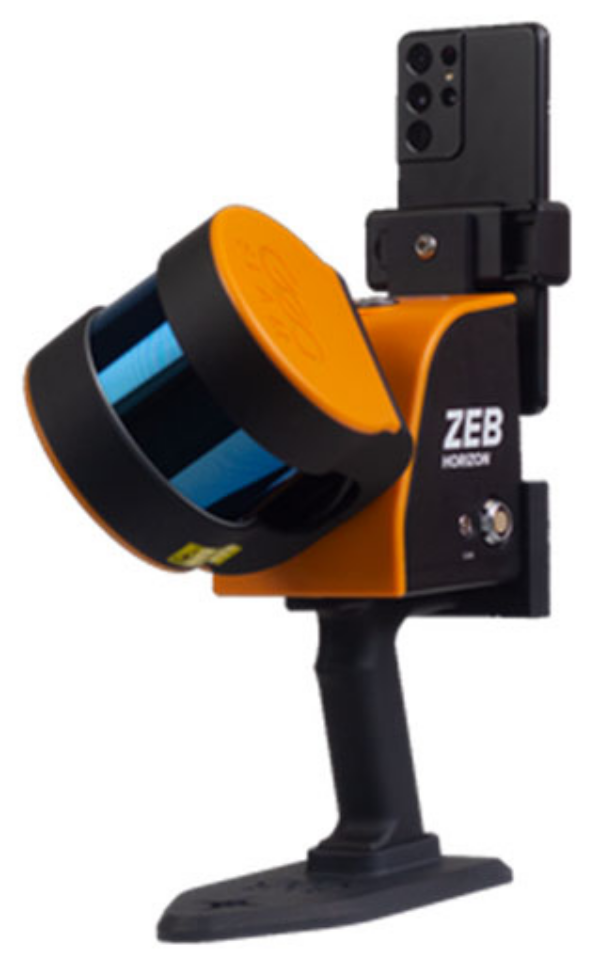
Handheld LiDAR System: The last system employed in this study is a handheld mobile laser scanning (MLS) system, specifically the GeoSLAM Horizon RT (FARO) shown in Figure 3. Unlike the UAV and BackPack systems that rely on GNSS/INS integration for direct georeferencing, this system utilizes a Simultaneous Localization and Mapping (SLAM) algorithm for trajectory estimation. The horizon sensor captures approximately 300,000 points per second with a range of up to 100 m, enabling rapid data acquisition in GPS-denied environments such as dense forest canopies. The raw data were processed using GeoSLAM Hub to generate the final point cloud.

3. Study Sites and Datasets Description

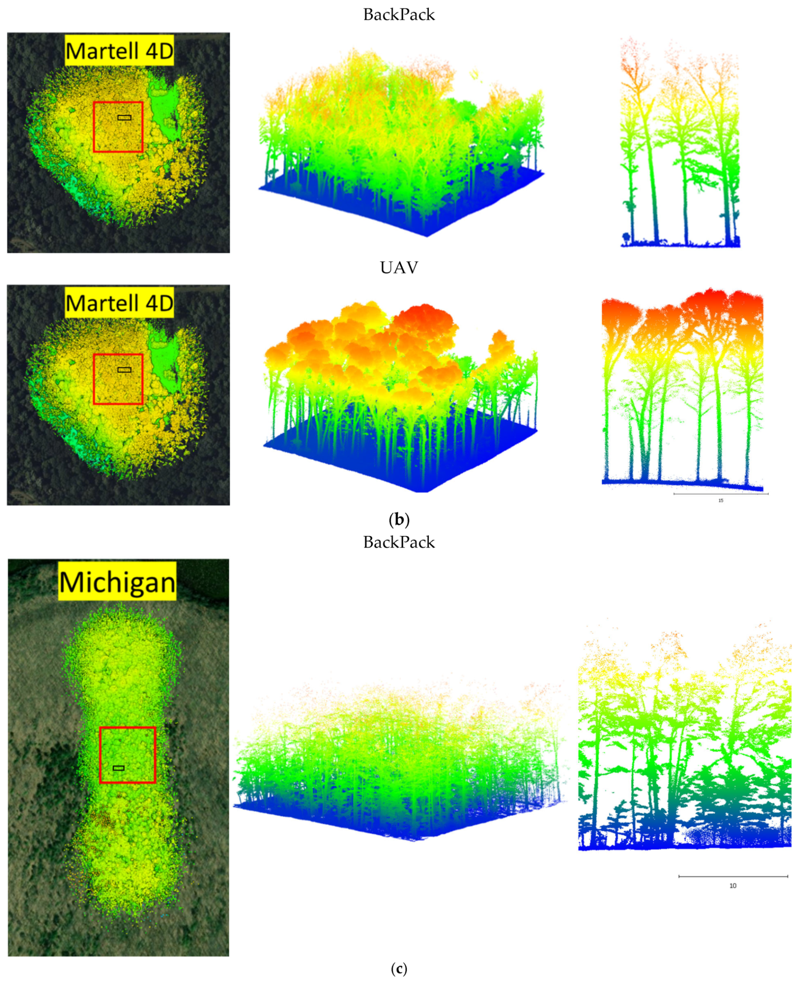
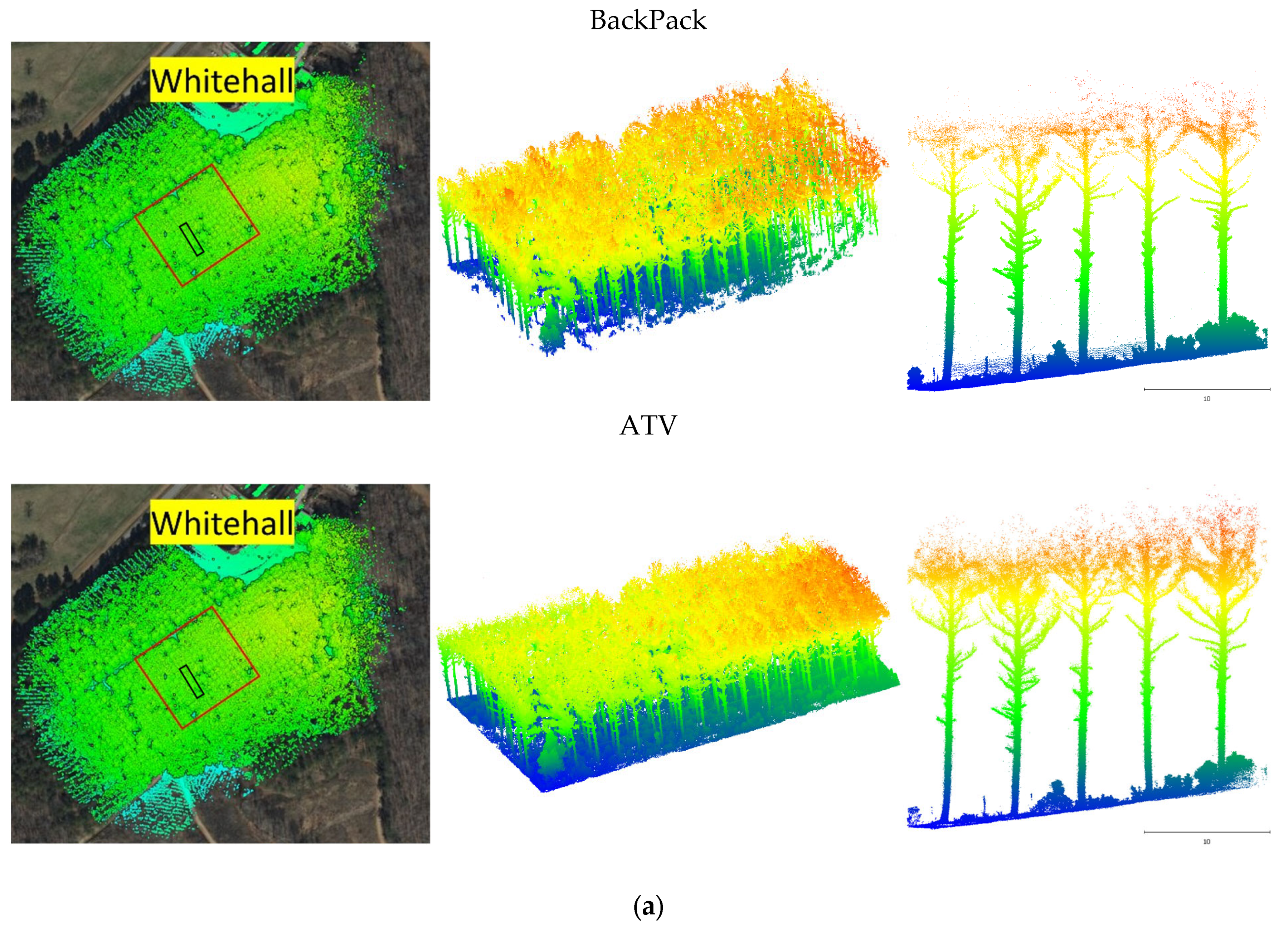
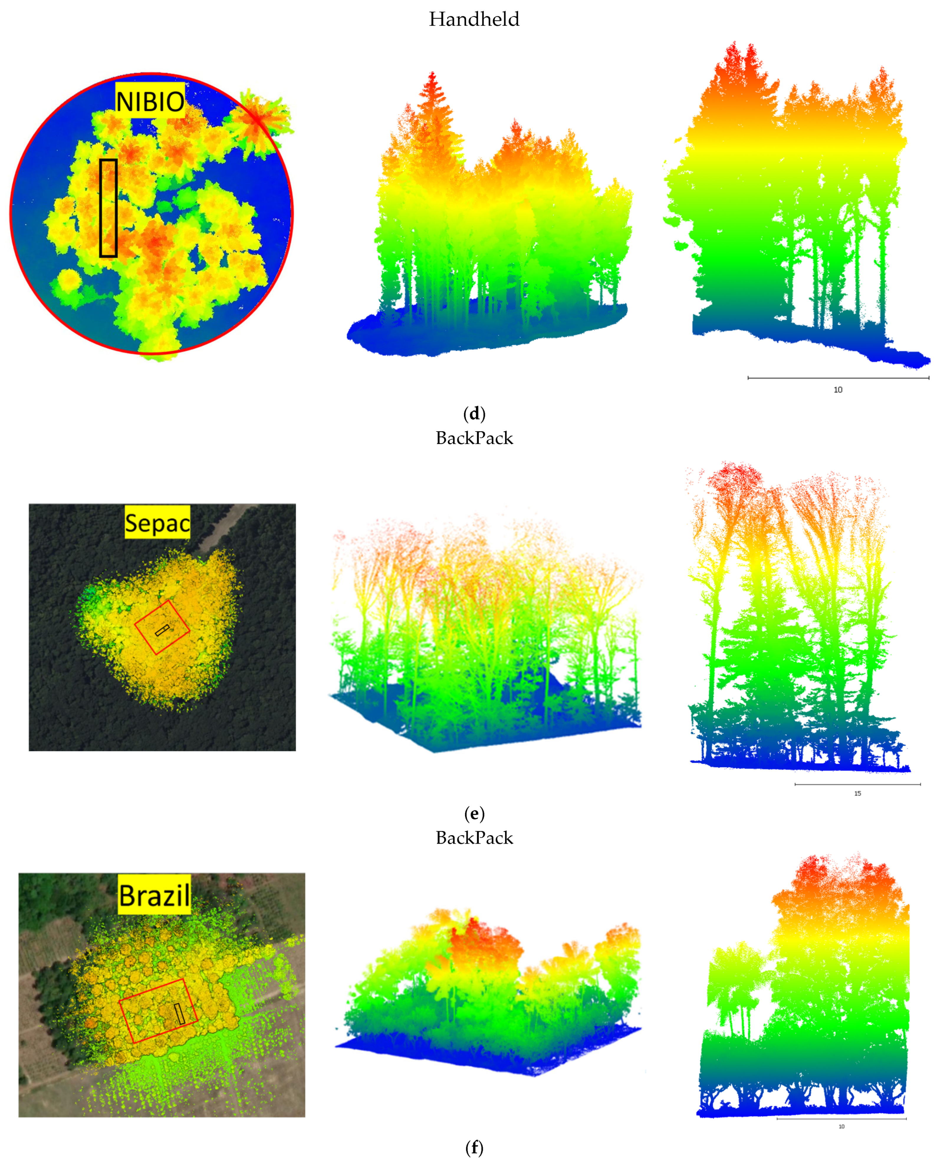
To evaluate the proposed pipeline under different forest structures and LiDAR acquisition conditions, eight ROI-level datasets collected from six study sites were assembled as diverse test cases. The sites span regularly spaced managed plantations, mixed-species temperate forests, a highly occluded single-pass transect, a dense boreal plot, a tropical environment, and natural forest with dense understory. Figure 4 shows the complete study sites and their region of interest (ROI) tiles used later for qualitative and quantitative analysis, while Table 1 summarizes key information on the datasets, including platform used, collection date, and total number of points.
Site 1: Whitehall Forest. Whitehall is a managed pine plantation located in Clarke County, Georgia, USA (33°53′04″N, 83°21′25″W). The ROI, highlighted in Figure 4a, is approximately 55 m × 50 m and is characterized by uniform tree spacing and minimal understory, providing a controlled setting for isolating platform effects. Two datasets were collected over the same ROI: (1) a pedestrian dataset acquired using the BackPack Knap-XP1 system, and (2) an ATV-based mobile mapping dataset acquired using the Knap-XP1-ATV configuration. Using two acquisition patterns, walking pace vs. vehicle-based, over the same plantation enables evaluation of the pipeline’s sensitivity to platform and trajectory variations in a low-complexity environment.
Site 2: Martell Forest. Martell 4D is a mixed-species natural forest located in West Lafayette, Indiana, USA (40°26′23″N, 87°02′01″W). The selected ROI, highlighted in Figure 4b, is approximately 55 m × 65 m and contains mature trees with heights in the range of ~24–28 m. Two datasets were acquired for cross-platform evaluation; a BackPack dataset collected using the E2HDL32E system and a UAV dataset. This site serves as the primary quantitative benchmark because it includes field reference measurements for individual tree locations and DBH, enabling rigorous assessment of detection and biometrics accuracy.
Site 3: Michigan Transect. This mixed forest site is located in Cheboygan County, near Pellston, Michigan, United States (45°33′54″N, 84°41′52″W). Situated in the transition zone between temperate and boreal forests, the site, highlighted in Figure 4c, contains a mixture of northern hardwood and conifer species within a 50 m × 50 m ROI. Knap-XP1 data were acquired to test the proposed pipeline’s performance on sparse, single-pass data with high occlusion.
Site 4: NIBIO Benchmark. This public benchmark dataset is provided by the Norwegian Institute of Bioeconomy Research (NIBIO). It represents a dense boreal forest environment dominated by coniferous species, highlighted in Figure 4d, within a circular plot of 25 m diameter. This dataset was acquired using MLS with a GeoSLAM Horizon RT sensor processed using GeoSLAM Hub. This dataset serves as the standard for testing the pipeline’s performance on high-density, handheld SLAM-based LiDAR data.
Site 5: SEPAC Forest. This natural forest is located within the Southeast Purdue Agricultural Center (SEPAC) in Jennings County, Indiana, USA (39°03′32″N, 85°32′31″W). Highlighted in Figure 4e, the site comprises a 50 m × 50 m ROI containing a diverse, complex mixture of hardwood species. Characterized by dense understory and difficult terrain, this site represents a structurally complex temperate forest environment. LiDAR data for the site was acquired using the BackPack system E2HDL32E.
Site 6: Brazil Açaí. This complex tropical site is located in the state of Pará, Brazil (2°21′52″S, 48°13′11″W). The study area, highlighted in Figure 4f, comprises a 40 m × 45 m ROI within an agroforestry system dominated by Açai palms. This site represents the most structurally challenging environment, featuring a multi-layered canopy with tall palms and an extremely dense, complex understory. The data were captured with the E2HDL32E system and serve as the primary test for the pipeline’s environment–agnostic capabilities in difficult tropical conditions.

4. Methodology

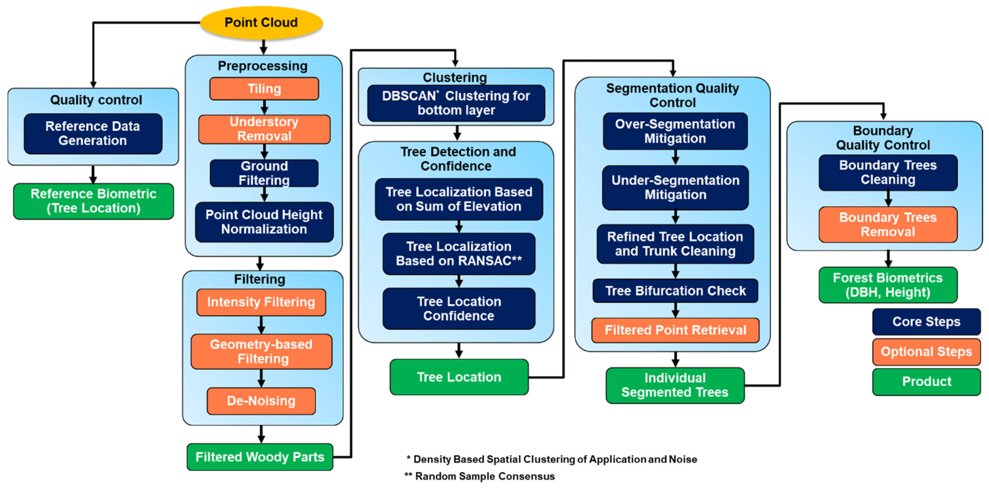
Figure 5 summarizes the two main branches of the proposed framework. The core processing branch converts the input point cloud into individual tree segments and derives forest biometrics through four principal stages: namely, preprocessing and woody point isolation, dual-method for tree localization, confidence-guided segmentation quality control, and filtered-point retrieval with boundary cleaning. The second branch provides a semi-automated procedure for generating reference tree locations for accuracy assessment when field measurements are unavailable. The following sections describe the implementation of these stages in detail.

4.1. Preprocessing

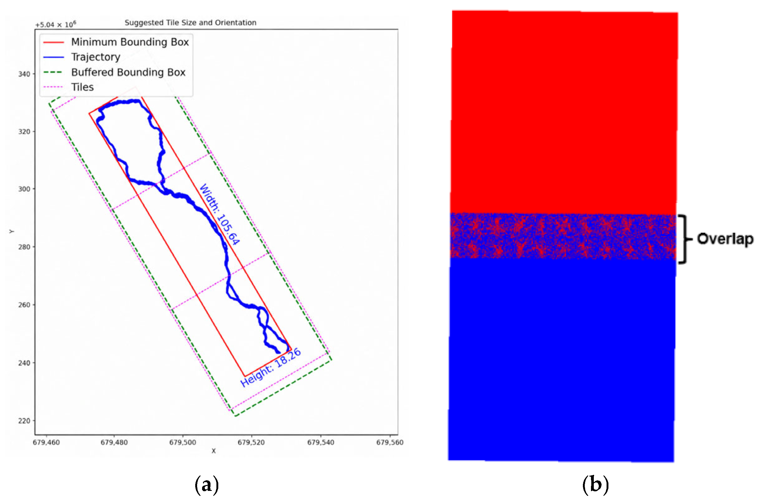
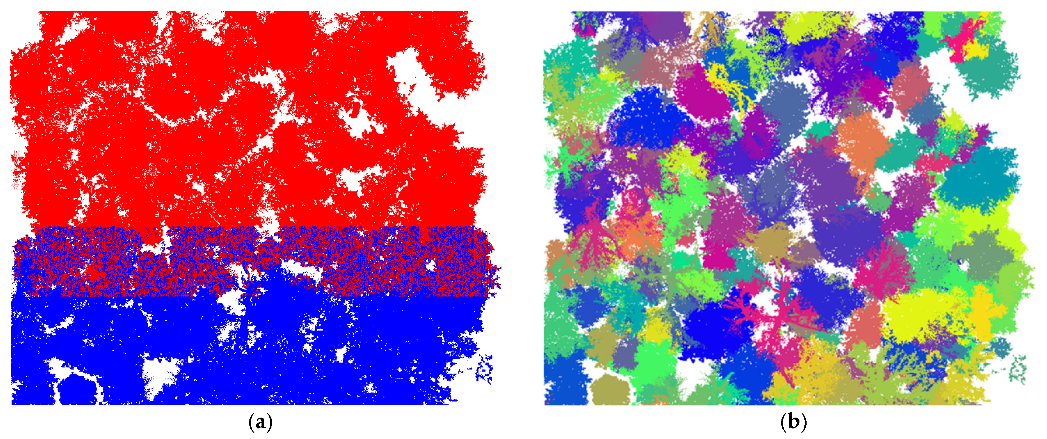
The preprocessing phase begins with point cloud tiling to ensure computational efficiency and enable the processing of large-scale datasets. The pipeline first partitions the full point cloud into tiles. This process begins by defining an ROI considering the system trajectory to exclude sparse, incomplete tree structures in the far field. An oriented minimum bounding box is generated around the trajectory and expanded by a user-defined trajectory buffer ( T b ), as shown in Figure 6a. For study sites containing datasets acquired by multiple platforms, the same trajectory was used to define the buffered ROI for all overlapping datasets. The resulting ROI extent and tile boundaries were therefore identical, ensuring that the cross-platform evaluations were conducted over the same area. The buffered ROI was then subdivided into a set of tiles, where the tile size was automatically selected from a predefined range between 30 m and 100 m to minimize the extension of the tiling beyond the ROI, and tiles were generated with a user-defined overlap distance ( O d ), as shown in Figure 6b. This overlap ensures that any tree located on or near a tile boundary is captured in its entirety within at least one tile.
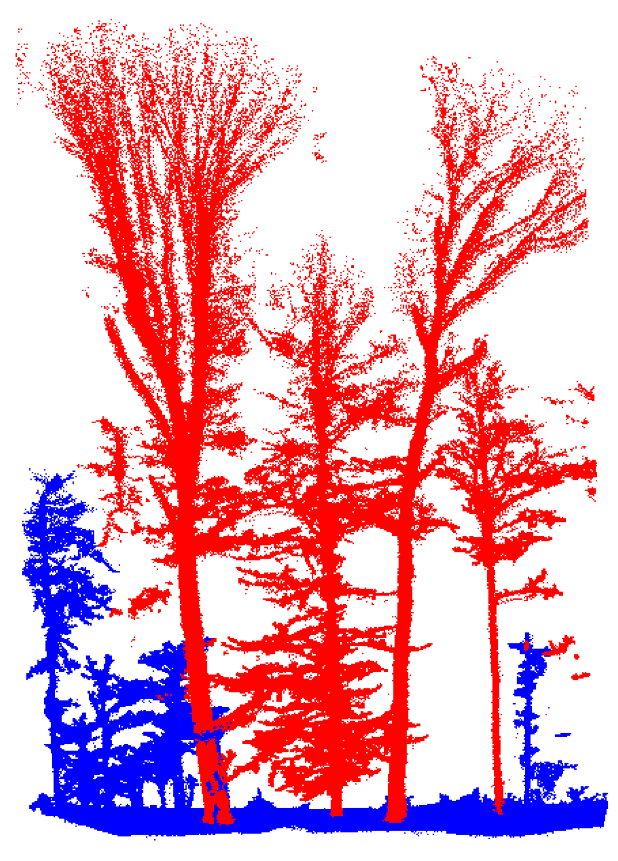
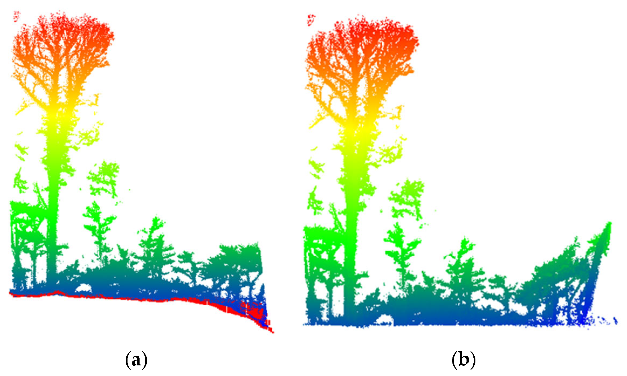
Following the tiling process, an optional understory removal step can be applied. The pipeline employs a sparse-convolution 3D U-Net to classify overstory tree points and understory vegetation, as shown in Figure 7. The model was pretrained on a large-scale 3D dataset [27] and subsequently adapted to forestry data by Shao et al. [28]. The forestry-adapted model was developed and evaluated using mobile LiDAR data from temperate natural forests with complex understory. Therefore, the temperate Martell-4D Forest used in this study is more similar to its original application domain. However, the plantation, boreal, and tropical datasets represent different forest structures. This difference is one reason the understory removal module is treated as an optional component rather than being applied universally. In the forestry training annotations, trees with DBH larger than 12 cm were classified as overstory trees, whereas ground, shrubs, and trees with DBH less than 12 cm were classified as understory. The same forestry-adapted model was used for all datasets in which understory removal was enabled, without dataset-specific retraining. Accordingly, the module is intended for inventories targeting larger or merchantable stems when dense low vegetation produces false stem candidates or connections between neighboring trees. The understory removal step should be disabled when small-diameter trees constitute valid inventory targets. No tree height threshold is used because the model classification was defined primarily according to DBH. Following understory classification, ground filtering is performed using an adaptive cloth simulation filter (CSF) to separate ground and non-ground points [29]. The cloth simulation generates a digital terrain model (DTM), which is used as a reference surface to normalize the heights of all above-ground points, converting absolute elevations to height above ground as shown in Figure 8.

4.2. Point Cloud Filtering

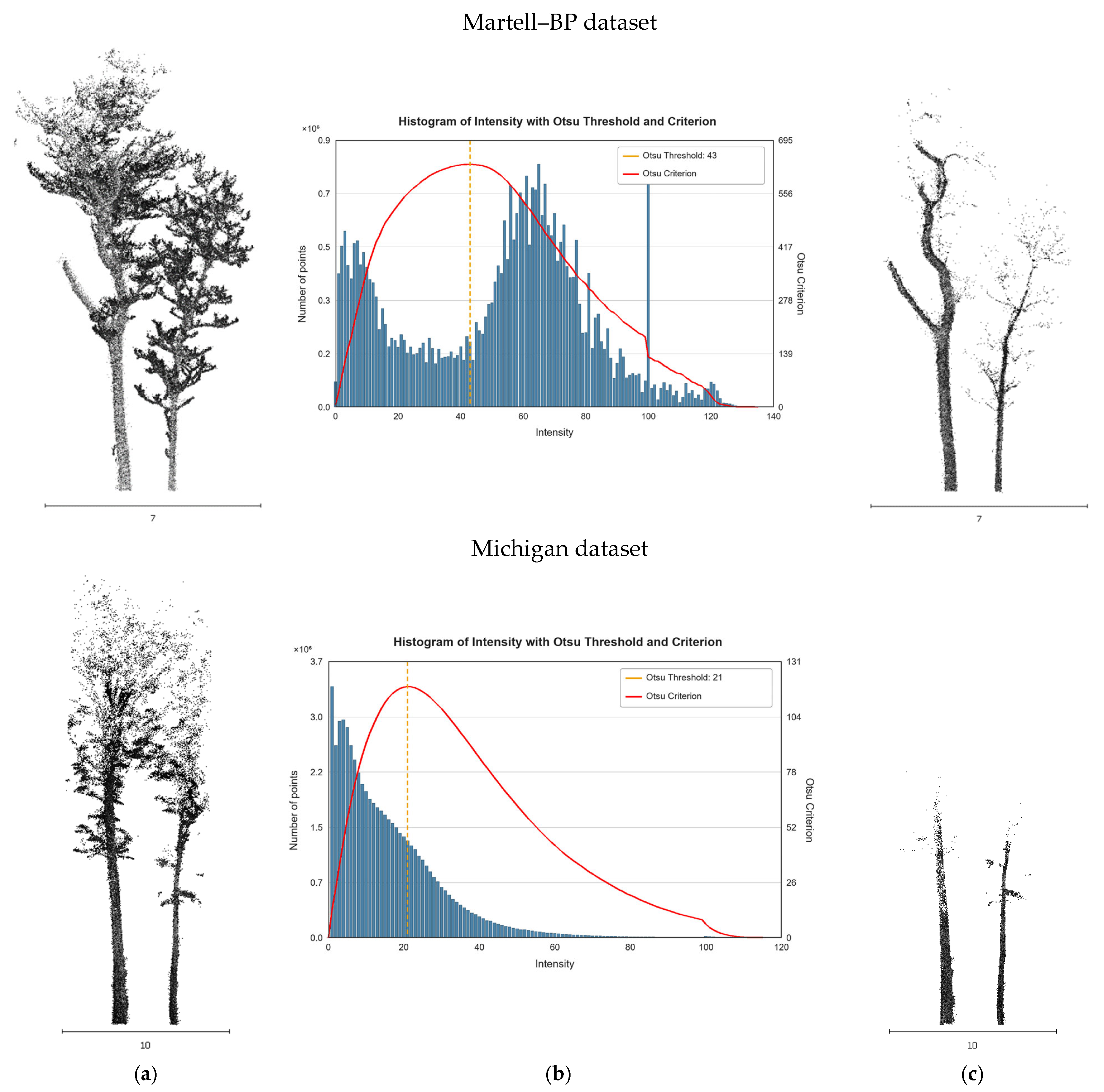
Following height normalization, three sequential filters are applied to isolate candidate woody points and reduce connections between neighboring trees before stem clustering. Specifically, intensity filtering, geometry-based filtering, and Statistical Outlier Removal (SOR) are discussed. First, Otsu’s method is applied independently to the intensity distribution of each dataset to separate candidate woody points from foliage [30]. Raw intensity values are not normalized or compared directly across sensors or datasets, and no universal threshold is used. Points below the dataset-specific threshold are flagged as filtered foliage points for later reassociation with the segmented trees, as shown in Figure 9.
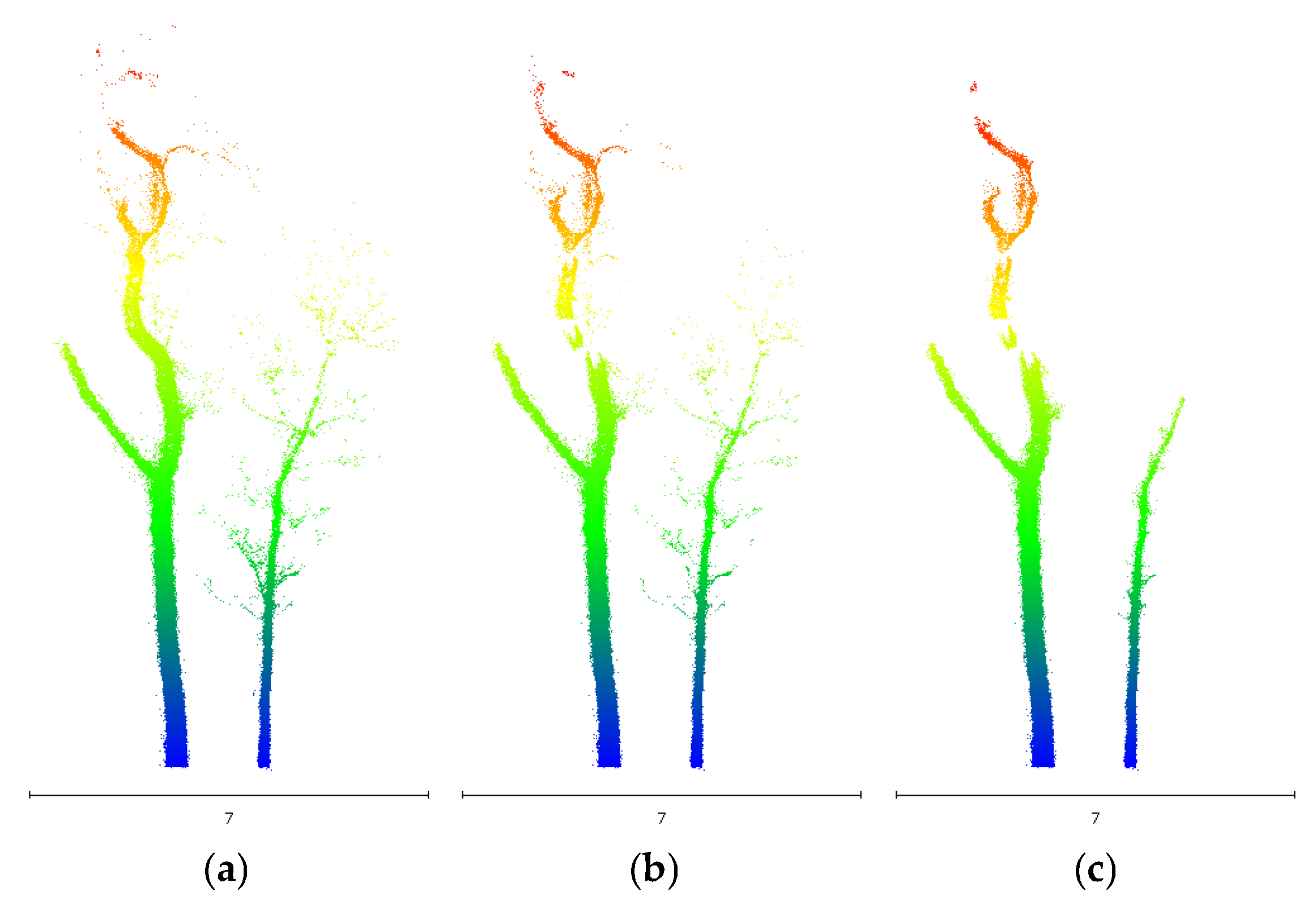
Next, the retained points are partitioned into prisms of size ( P l , P w , P h ), and a linearity measure is calculated from the eigenvalues of the local covariance matrix. Prisms below the defined linearity threshold are removed, preserving elongated structures associated with stems and major branches. Finally, SOR removes isolated points that are inconsistent with the local woody structure. Figure 10 shows the progressive output of these three filtering stages, while the corresponding parameter values are reported in Table A2.

4.3. Initial Stem Clustering

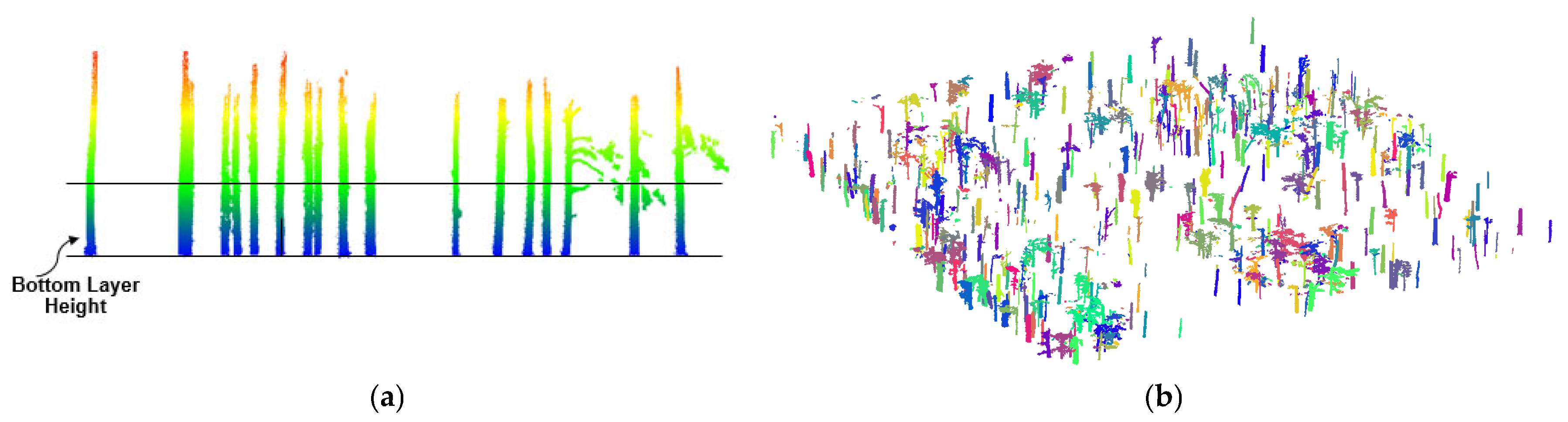
Following the filtering stage, the denoised, height-normalized point cloud of woody components is used to generate initial stem clusters. Clustering is performed using the Density-Based Spatial Clustering of Applications with Noise (DBSCAN) algorithm [31], as shown in Figure 11. This strategy focuses on the tree trunks, which are the most geometrically distinct and separated features. This reduces interference from interlocking branches and upper-canopy structures. Using the neighborhood radius (epsilon) and minimum point count (MinPts), DBSCAN groups spatially connected woody points into candidate trunk clusters, as shown in Figure 11b. These clusters are then passed to the dual-method tree localization stage.

4.4. Tree Detection and Localization

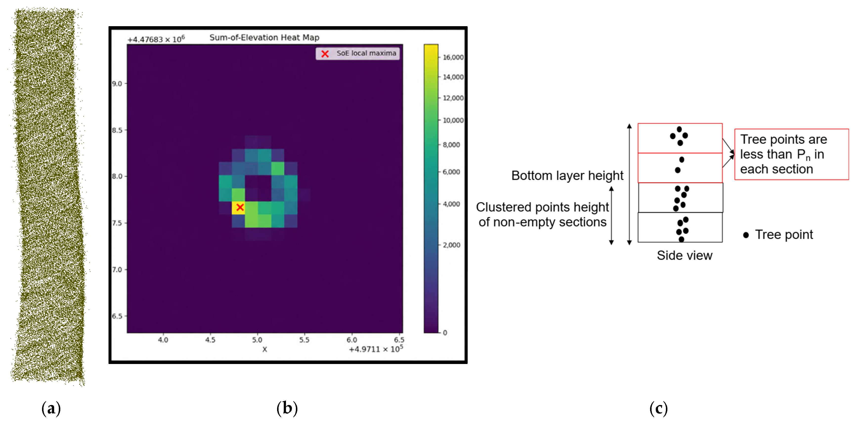
Once the initial trunk clusters have been generated, the proposed tree detection strategy executes two algorithms in parallel to identify tree locations. These methods focus on different tree attributes, specifically vertical structure and cylindrical shape, to assign a confidence level to the detected tree locations. The first localization method is the Sum of Elevation (SoE) approach. For each candidate trunk cluster, the points are projected onto a two-dimensional horizontal grid, and the normalized heights of all points within each grid cell are summed. A vertically continuous stem contributes points at the same horizontal coordinates over multiple heights, producing a high accumulated value and a distinct local peak in the SoE heat map. In contrast, branches and understory points are generally more horizontally dispersed or less vertically continuous and therefore produce weaker or less spatially consistent responses. The grid cell corresponding to each retained peak is taken as a candidate tree location, as shown in Figure 12a,b. To suppress false positives, which are often caused by low shrubs that may pass the initial filtering, a trunk continuity check is applied. The full cluster is partitioned vertically into several sections ( N s ), as shown in Figure 12c. A section is considered empty if it contains fewer than a predefined minimum number of points ( P n ). A candidate location is rejected as a false positive if it fails to exhibit sufficient vertical continuity. Specifically, rejection occurs if the maximum height of contiguous non-empty sections falls below a minimum threshold ( C h ) or the empty ratio (empty sections/total sections) exceeds a maximum tolerance ( E r ). Candidate peaks that satisfy these continuity criteria are retained as initial tree locations.
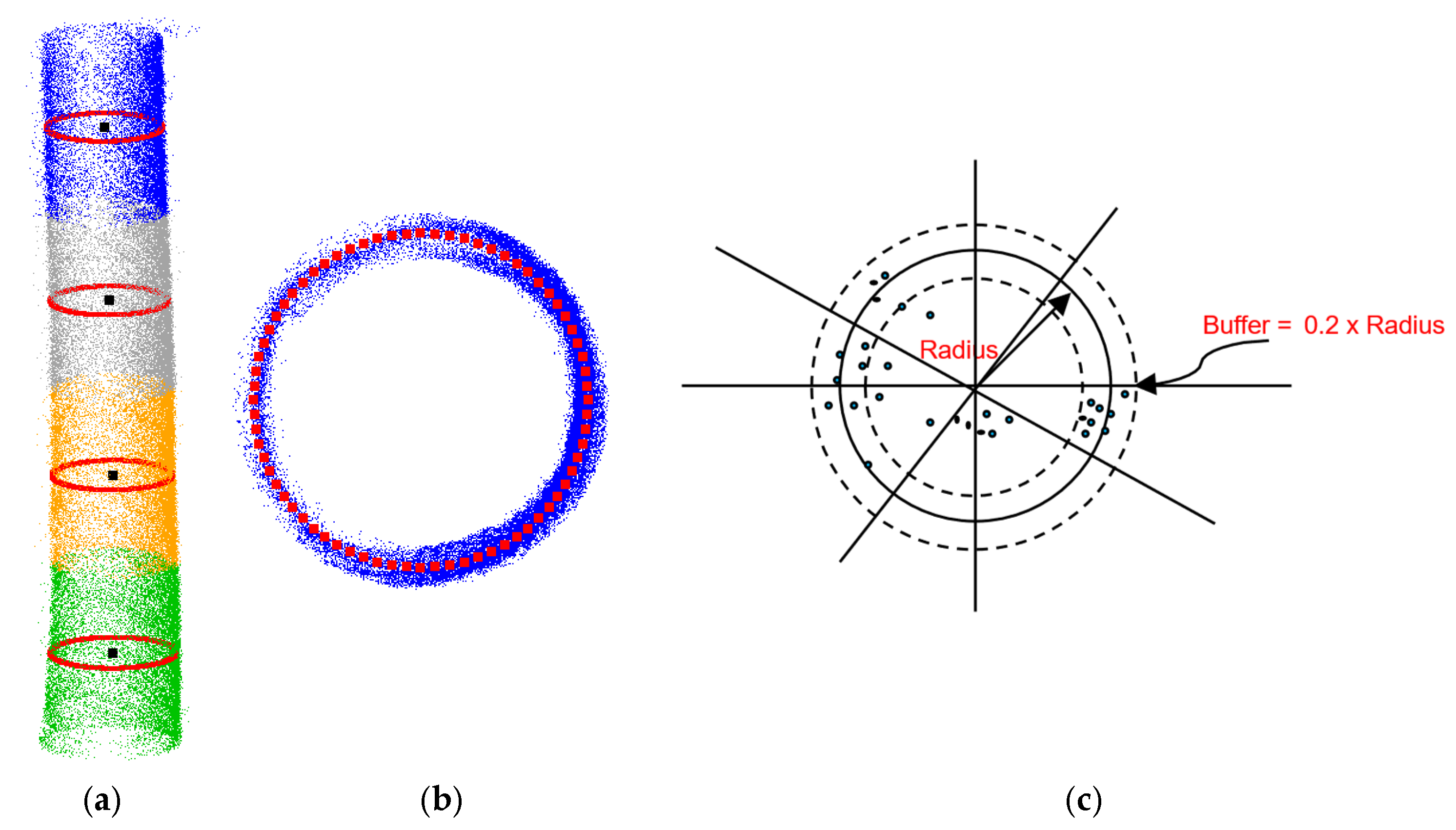
In parallel, the second localization method in the dual stem detection framework is then applied to the same DBSCAN trunk clusters. This approach uses a RANSAC-based circle fitting algorithm [32] to identify and validate the cylindrical shape of the stems. Each cluster is partitioned vertically into multiple sections ( N s ), as shown in Figure 13a. For each section, points are projected onto the horizontal plane, and a circle is iteratively fitted. To improve robustness against noise and occlusion, each fitted circle is evaluated using several quality control criteria. These include the permissible radius range [ T m i n , T m a x ], the maximum allowable fitting RMSE ( T f ), the minimum number of points within the section ( P n ), and a cross-sectional completeness percentage ( C p ) to reject partial arcs caused by occlusion. Completeness ( C p ) is quantified by defining a buffer (e.g., 20% of the radius) around the fitted circle and subdividing this buffer into angular sectors, as shown in Figure 13b. The algorithm checks for point existence within each angular sector and counts the largest number of continuously occupied sectors to determine the final completeness percentage. This process yields a set of high-confidence 2D circle centers from the sections that pass all quality checks. Because each trunk cluster is divided into multiple vertical sections, multiple circle centers are typically obtained for the same stem in the (X, Y) plane. These centers are then clustered using DBSCAN to merge spatially consistent centers. If multiple spatially distinct centers are found within the same DBSCAN trunk cluster, more than one initial tree location is retained, allowing potential under-segmentation cases to be identified. The mean location of each cluster containing at least a minimum number of centers (e.g., more than 2) is accepted as an initial tree location.
The pipeline combines the outputs of the SoE- and RANSAC-based localization methods to assign a detection confidence value, under the hypothesis that detections from both methods are more reliable. A location is considered matched when the 2D Euclidean distance between the two location estimates is smaller than a predefined matching threshold ( M t h ). Matched detections are assigned an agreement level of 2, while detections identified by only one method are assigned an agreement level of 1. If both methods detect a tree within the same cluster but estimated locations diverge beyond the matching threshold ( M t h ), the RANSAC-derived location is retained with assigned agreement level of 1. Both agreement levels are retained for the subsequent quality control steps, while the assigned value indicates the strength of the supporting stem location evidence.
Matched detections from both SoE- and RANSAC-based localization are considered high-confidence tree locations because they are supported by both vertical continuity and cross-sectional stem geometry. In contrast, detections identified by only one approach are retained as lower-confidence tree location evidence. These lower-confidence detections are not removed automatically; instead, they are treated as indicators of potential segmentation ambiguity and are passed to the subsequent quality control stage for further evaluation.

4.5. Clustered Stem Quality Control

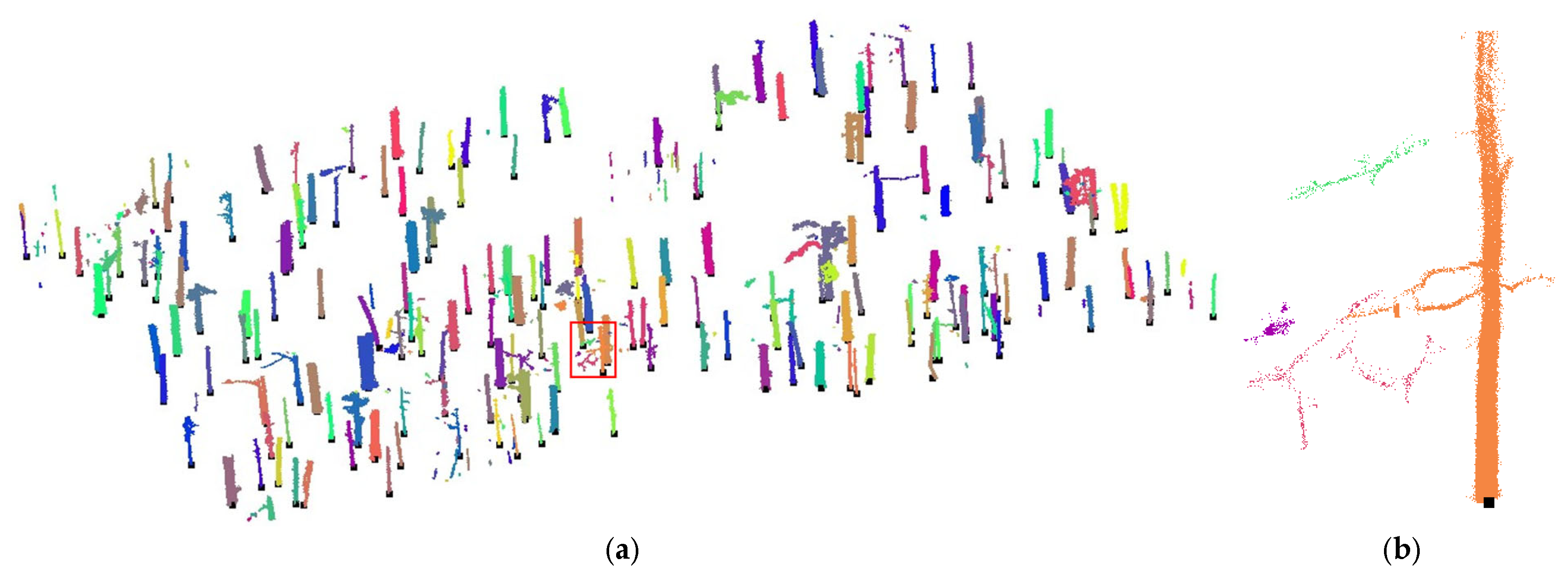
Following the dual tree detection phase, the detected tree locations and their assigned confidence levels are used to guide a multi-stage quality control module for correcting common clustered-stem errors that are prevalent in forest data. The first stage targets over-segmentation, where dense branching structures or residual noise persist through the filtering phase and are clustered by DBSCAN as distinct objects. As illustrated in Figure 14a, the detected tree locations are overlaid on the initial stem clusters. This constraint ensures that only clusters containing a stem detection with high confidence are retained. Clusters with no corresponding tree location are flagged as filtered points (Figure 14b).
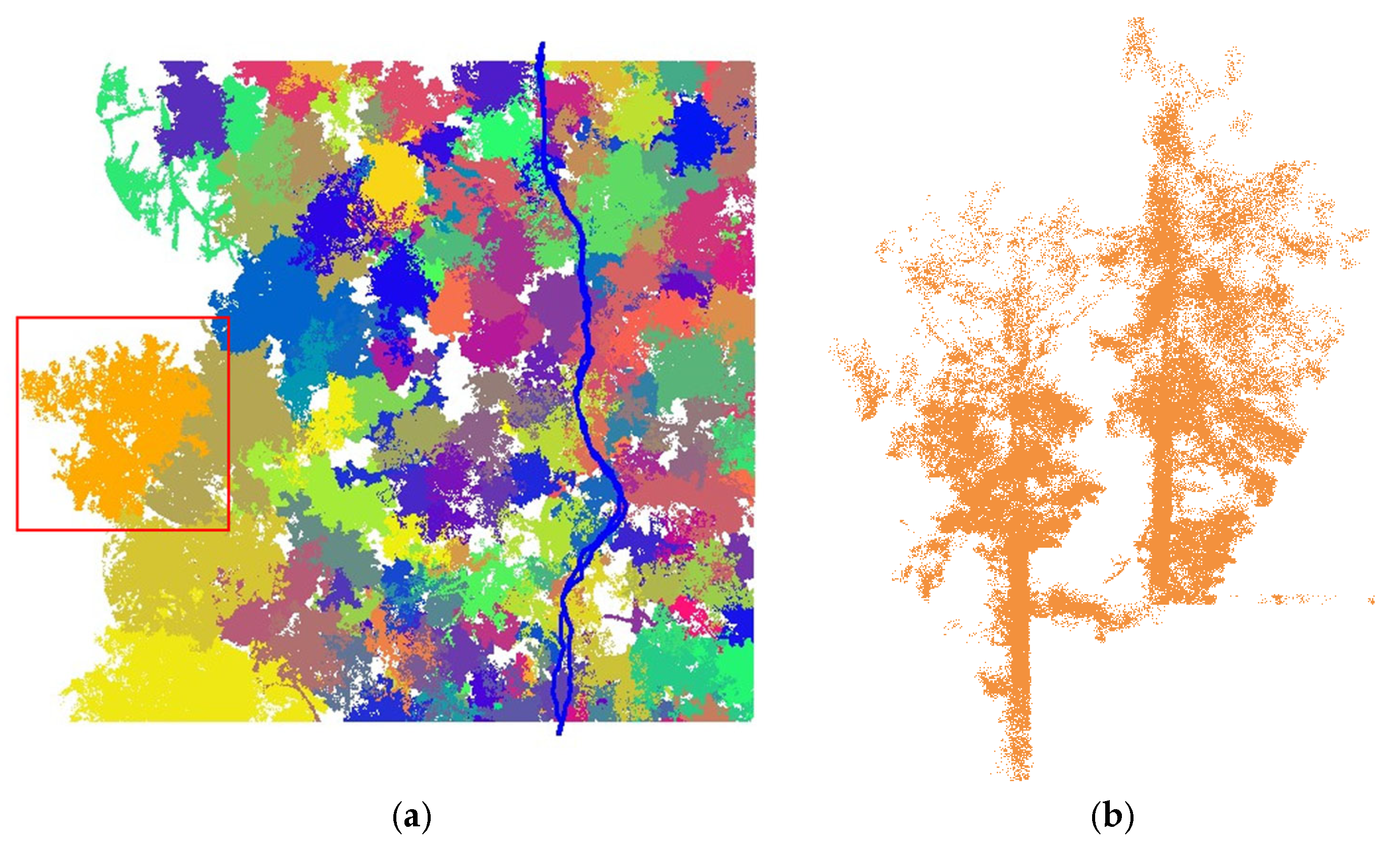
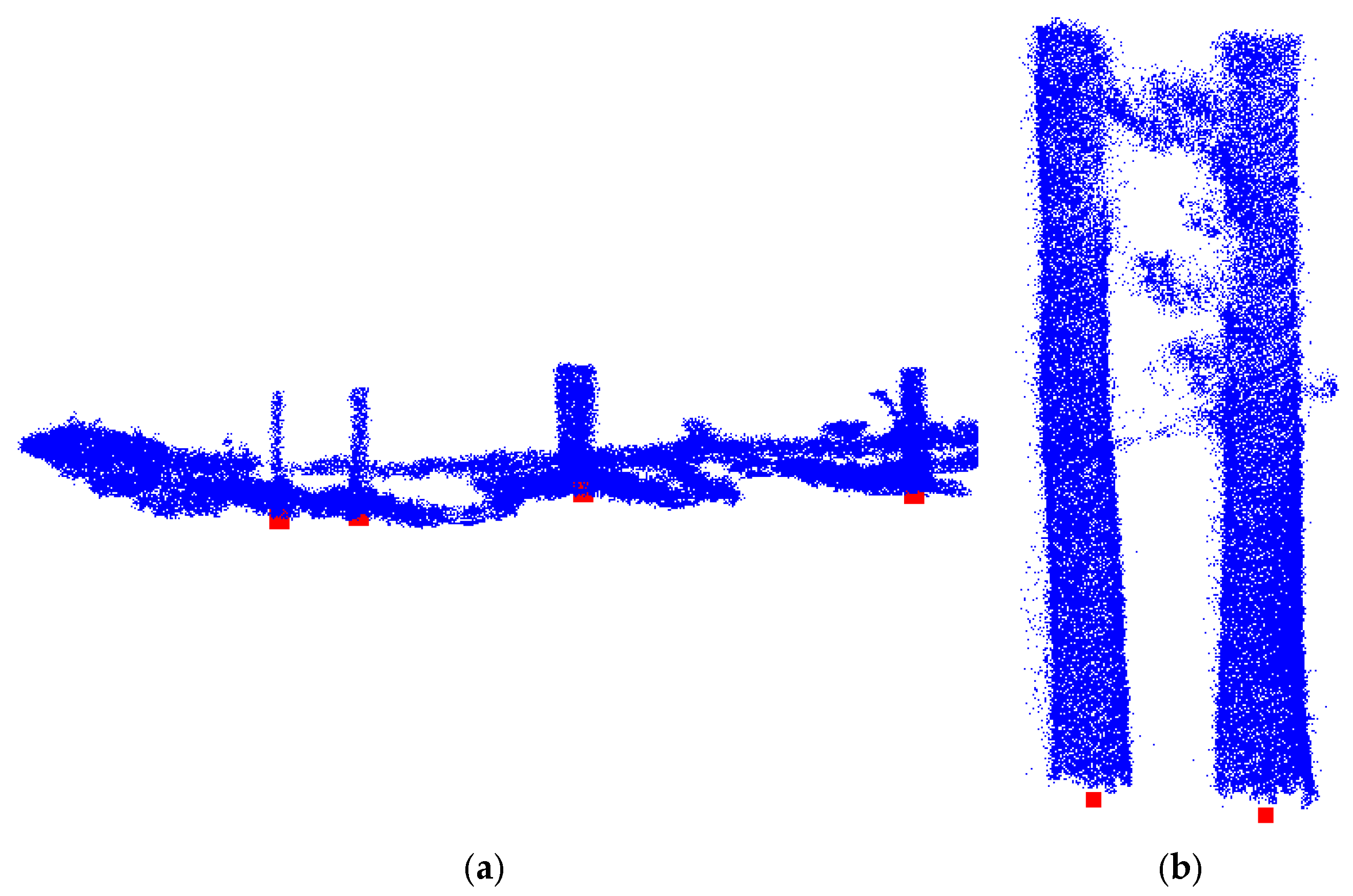
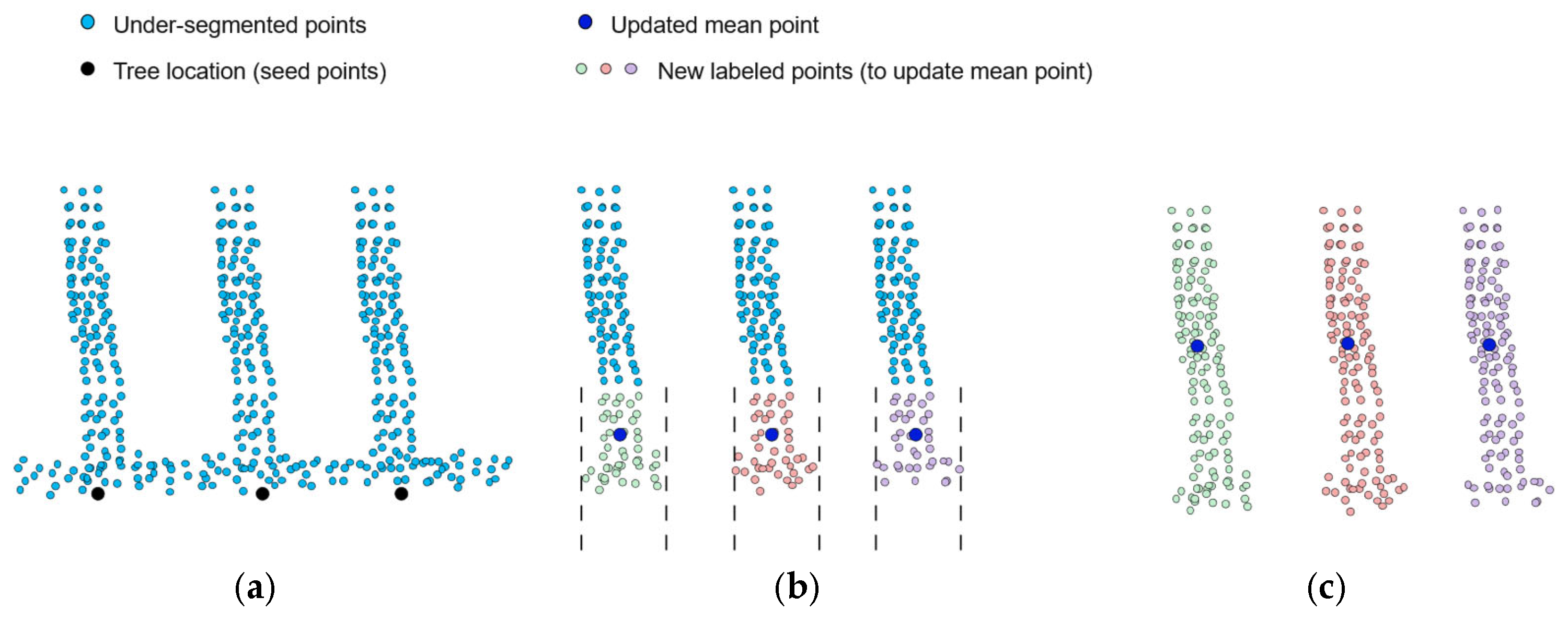
The next quality control step addresses under-segmentation, which occurs when a single DBSCAN cluster incorrectly contains multiple trees. The hypothesis is that these clusters have a large 2D extent and contain more than one confirmed tree location from the dual-tree detection stage. To identify these cases, the 2D minimum-bounding rectangle area is calculated for all clusters. A cluster is flagged as under-segmented only when both following conditions are satisfied: (1) its 2D area is large, and (2) it contains multiple tree locations, as shown in Figure 15. Once an under-segmented cluster is identified, a modified distance-based region growing algorithm is employed to split it [19]. The procedure initiates by sorting the cluster’s points by Z-coordinate to facilitate a bottom–up segmentation approach. A bottom–up strategy is adopted because the detected tree locations provide high-confidence seed points near the stem base, whereas a top–down approach is less reliable because neighboring trunks can converge or become connected in the upper section and make seed point definition ambiguous, as shown in Figure 15b. The detected tree locations serve as the initial seed points. To prioritize stem geometry, a spatial constraint is imposed wherein points exceeding a maximum 2D Euclidean distance (e.g., 0.5 m) from the seed points are excluded as illustrated in Figure 16b. The algorithm then iterates through the sorted list, assigning each point to the cluster of its nearest seed point. To accommodate stem curvature and lean, the cluster centroids are dynamically updated after a defined batch of point assignments. This adaptive mechanism ensures that the growth direction accurately follows the trunk structure, effectively resolving the fused cluster into distinct tree instances, as shown in Figure 16c.
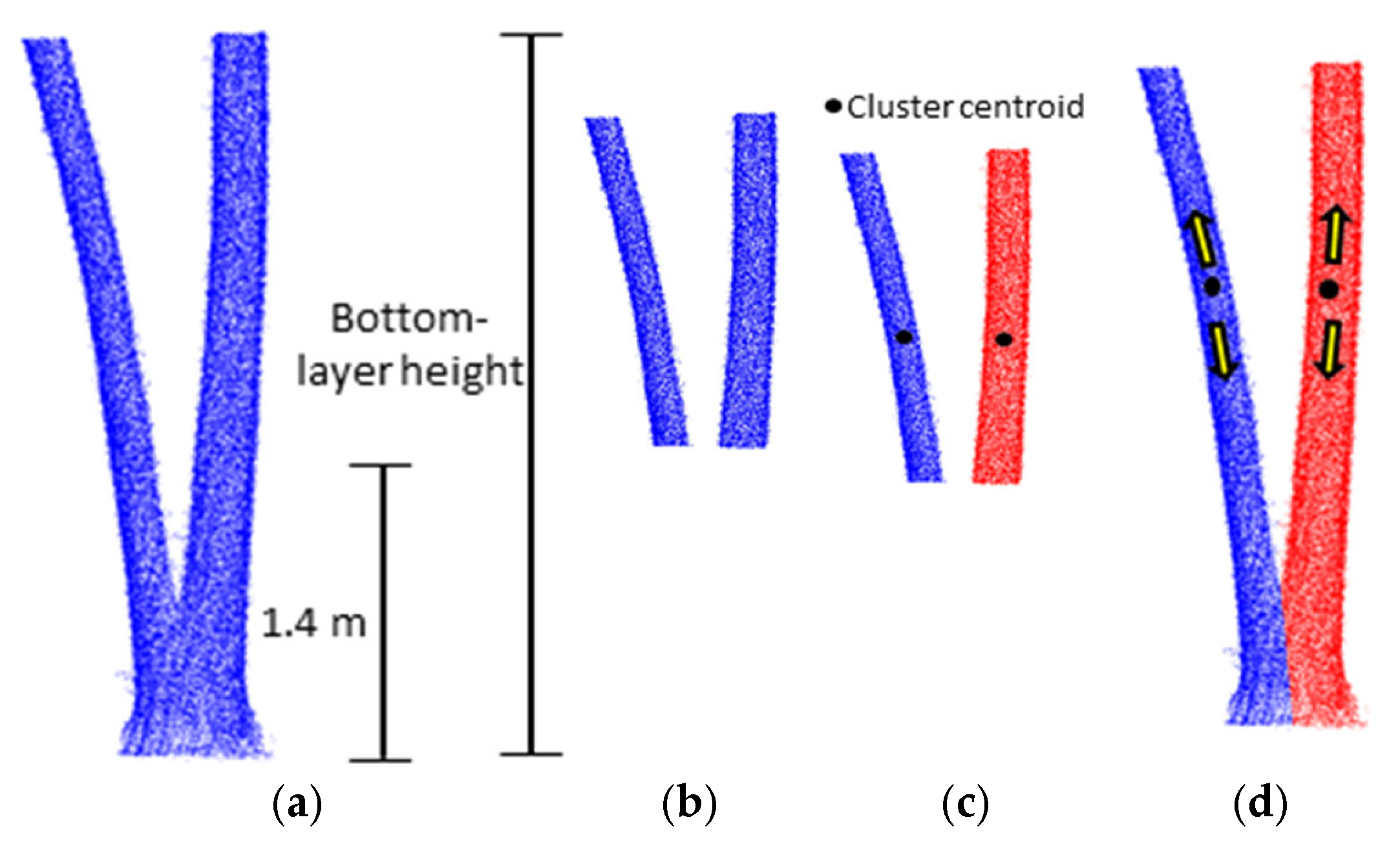
The next quality control step deals with multi-stemmed trees by isolating points within the height interval from 1.4 m to the same bottom-layer height previously used for DBSCAN clustering, as shown in Figure 17. DBSCAN clustering is then applied to this upper-trunk section to assess structural continuity. If a single cluster is identified, the tree is classified as single-stemmed; conversely, the emergence of multiple clusters indicates a multi-stemmed structure. These distinct stems are then segmented using the centroids of the identified DBSCAN clusters as new seed points. From each centroid, region growing proceeds bidirectionally, extending both upward and downward through the point set to separate the individual stems.
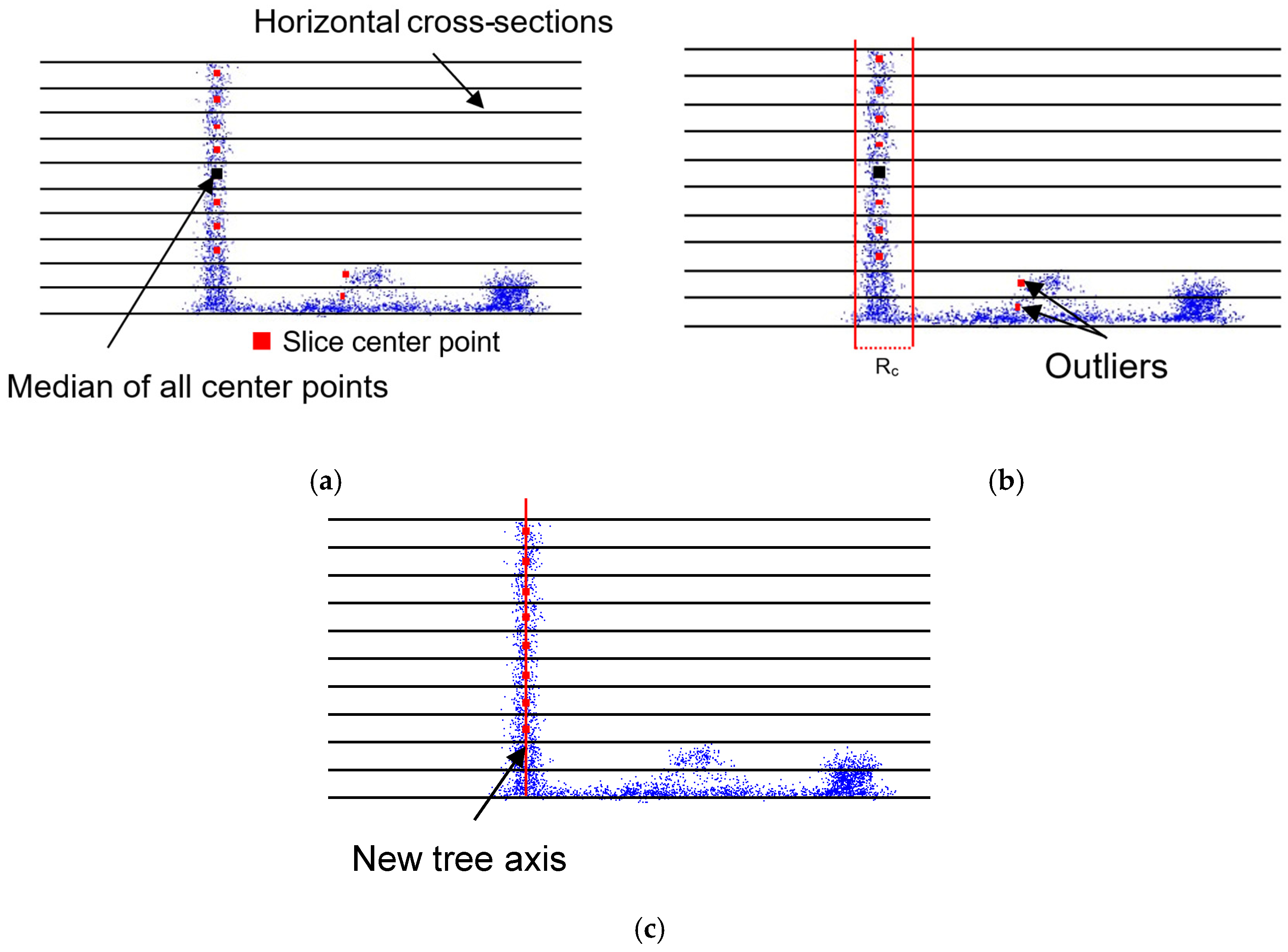
After stem segmentation, each trunk undergoes a final cleaning and refinement process. This step is essential to define a single, precise axis for the tree and remove small branches that may be attached to the trunk. The process starts by slicing the clustered tree trunks into multiple horizontal cross-sections ( S c ), as shown in Figure 18a. The slice localization process first uses circle fitting when the cross-section of the slice is sufficiently well defined, and otherwise uses a median-based estimate for sparse or incomplete data. The algorithm first attempts to fit a RANSAC circle to the points within the horizontal slice. If the cross-section confidence exceeds the threshold C t h , the center of the fitted circle is adopted as the slice location. Conversely, if the confidence falls below this threshold due to insufficient or fragmented point coverage, the RANSAC result is discarded. In such instances, the algorithm uses the median (X, Y) coordinate of the slice points as an approximation of the stem center. As shown in Figure 18b, the median (X, Y) location is computed from all retained slice center estimates, including both RANSAC-derived circle centers and median-based slice centers. Subsequently, any slice center whose 2D distance from this median point exceeds a defined threshold ( R c ) is classified as an outlier and discarded. This step effectively removes outlier centers caused by attached branches. The remaining inlier centers are then used to define the axis of the tree, as shown in Figure 18c.

4.6. Filtered Point Retrieval

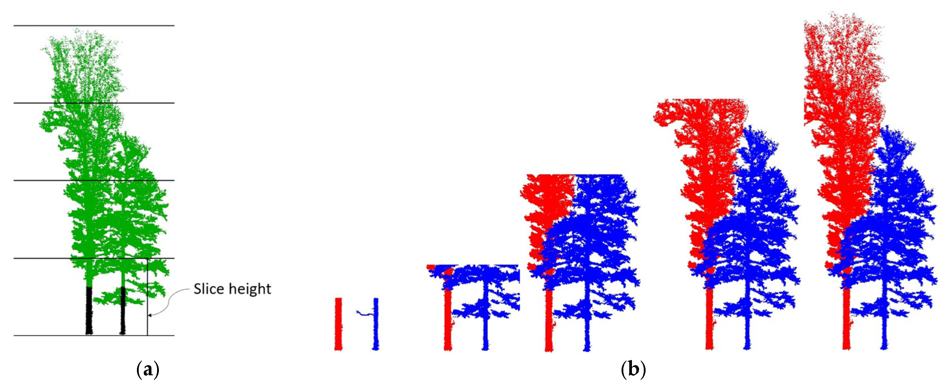
Following the isolation and refinement of the tree trunks, the pipeline proceeds to the filtered point retrieval stage. The objective of this step is to recover the non-woody points (foliage and small branches) that are removed during the initial filtering and reassociate them with their corresponding segmented trunks. This is critical for deriving total tree height and crown dimensions. To optimize the processing efficiency for large datasets, the entire filtered point cloud is first voxelized with a defined resolution ( V s ). This process allows the algorithm to perform distance queries using voxel centers rather than raw points, substantially reducing the search space. Furthermore, to avoid constructing a massive, memory-intensive KD tree for the entire voxelized scene, the point cloud is partitioned into horizontal slices of a defined height ( S h ) and each section is processed sequentially, as shown in Figure 19a. The retrieval process itself is implemented as an iterative region growing operation that begins with the validated trunk points as the initial seed. Within each vertical slice, a KD tree is built from voxel centers, and the algorithm queries all filtered points that are within a small search radius ( R i ) of the current seed points. These retrieved points are assigned the corresponding tree ID and added to the seed points for the next iteration. The segmentation expands outward dynamically, capturing attached foliage and branches through a continuous growing process, as illustrated in Figure 19b. The iteration for a given slice stops when a full pass retrieves no new points, or when a maximum iteration cap is reached. This process is then repeated for the next horizontal slice, efficiently growing the full tree structure from the bottom up.

4.7. Tile Boundary Quality Control

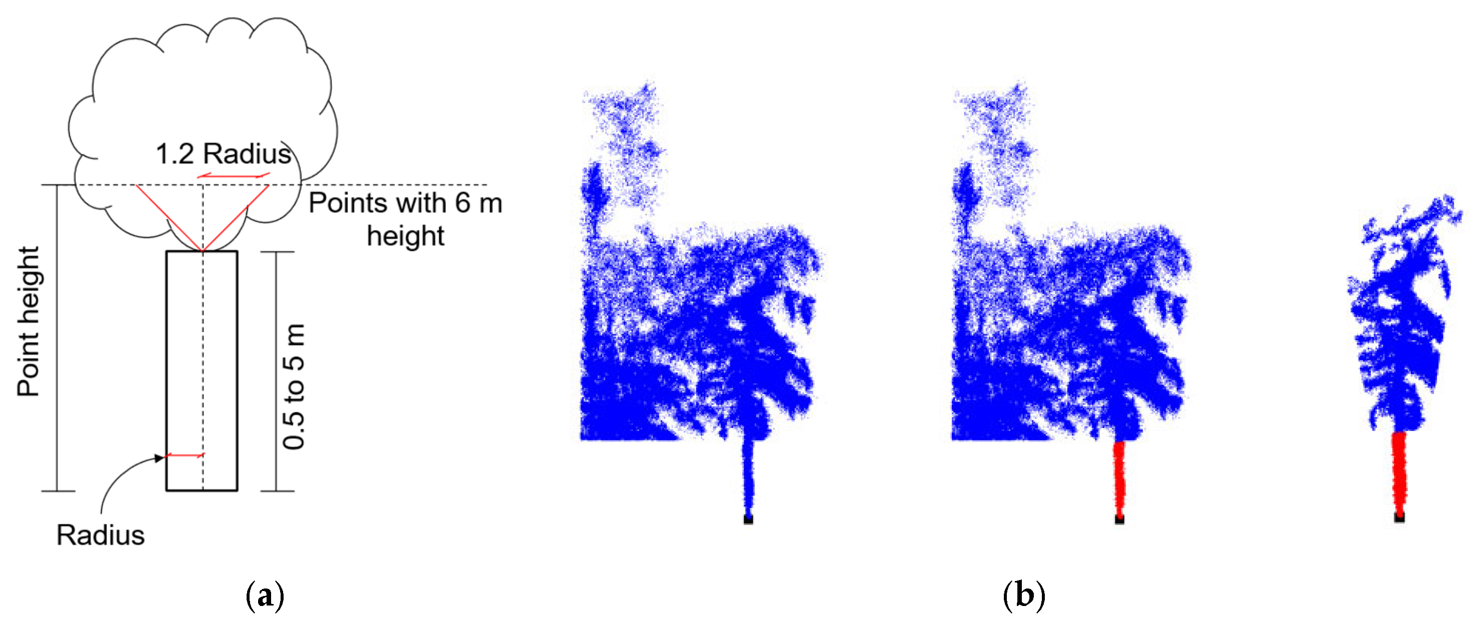
The final processing stage involves quality control steps to remove redundant trees arising from the tile overlap zones (Section 4.1). It begins with a boundary cleaning step designed to handle a specific type of under-segmentation common in sparse and incomplete data, particularly for trees far from the sensor trajectory, as shown in Figure 20. Abnormal trees are identified using the same logic for under-segmentation check discussed in Section 4.5. After the filtered point retrieval step, the 2D minimum-bounding rectangle extent is calculated for all segmented trees, and the median 2D extent is determined. A tree is flagged as abnormal if the following conditions are satisfied: (1) its 2D foliage footprint exceeds the median value, and (2) it contains only one detected trunk location. This combination identifies cases in which sparse foliage from adjacent, undetected sparse tree trunks have been erroneously merged into a single retrieved tree during the filtered-point retrieval step. To correct this, the foliage is refined using a height-dependent growing filter, as illustrated in Figure 21a. This method defines a maximum horizontal distance ( D t h ) that increases with the normalized height of each point ( h p ), mimicking the natural widening shape of a tree crown. The relation is mathematically defined by Equation (1). As a result, the filter preserves valid points near the trunk while removing distant points belonging to neighboring trees, as shown in Figure 21b, producing a clean individual tree.
D t h = R a d i u s , 0.5 h p 5 R a d i u s     1 + h p 5   0.2 , h p > 5  
The final step removes duplicate trees generated by the overlapping tile buffer size ( T b s ). As shown in Figure 22, trees located within adjacent tile-overlap zones are compared spatially, and detections falling within a defined proximity threshold are treated as duplicates. For each duplicate group, only the tree with the largest number of points is retained, assuming that it represents the most complete capture of the tree. This step ensures that each tree appears only once in the final inventory.

4.8. Generation of Reference Data for Accuracy Assessment

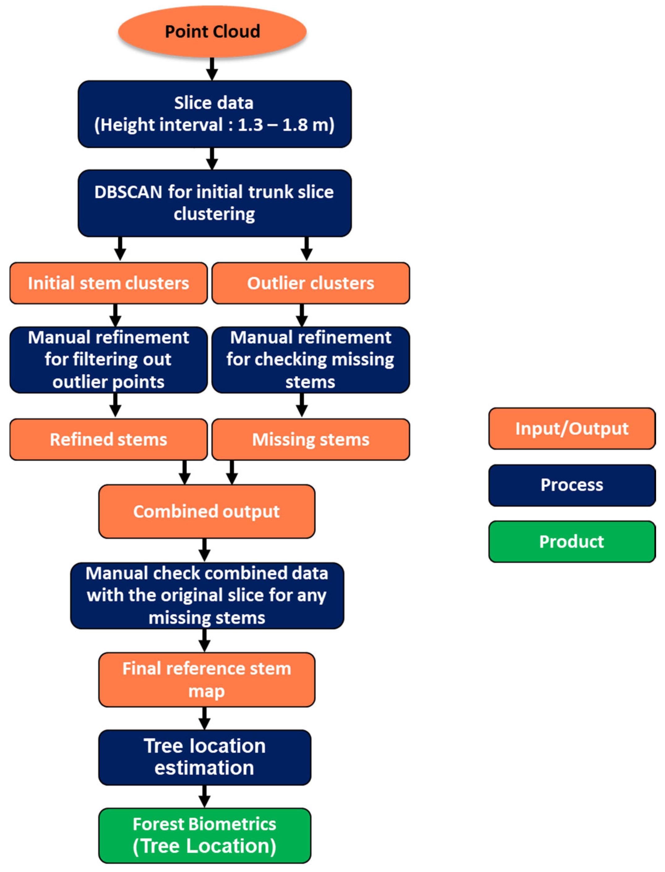
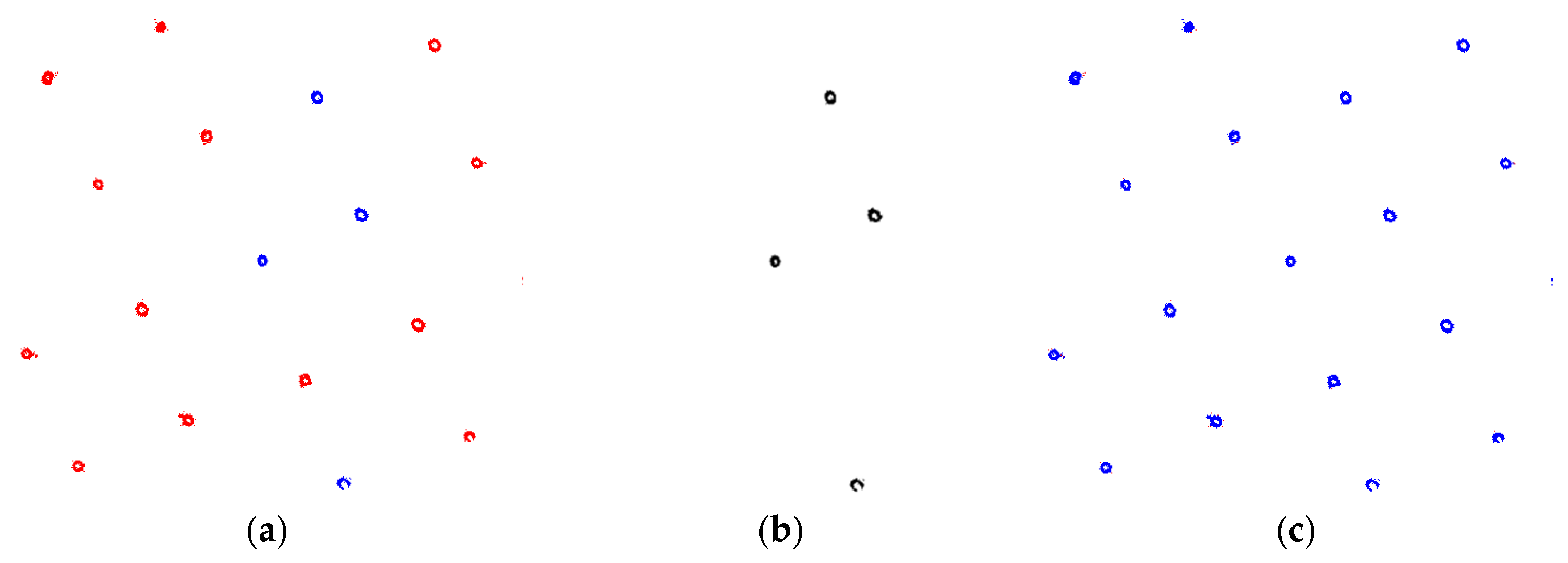
For datasets without field measurements, a reference dataset was generated using the semi-automated workflow shown in Figure 23. This procedure derives tree locations directly from the reconstructed point cloud through automated stem isolation followed by manual refinement. The resulting reference data were reviewed by three operators, and any disagreements were resolved through consensus. This procedure supports quantitative evaluation where field measurements are unavailable. It is not equivalent to independent field validation as the reference data have been generated from the same point cloud used for testing. The procedure is executed through three sequential steps: (1) an automated stem isolation using horizontal cross-section slicing and density-based clustering, (2) manual refinement of the detection results, and (3) final estimation of tree locations.
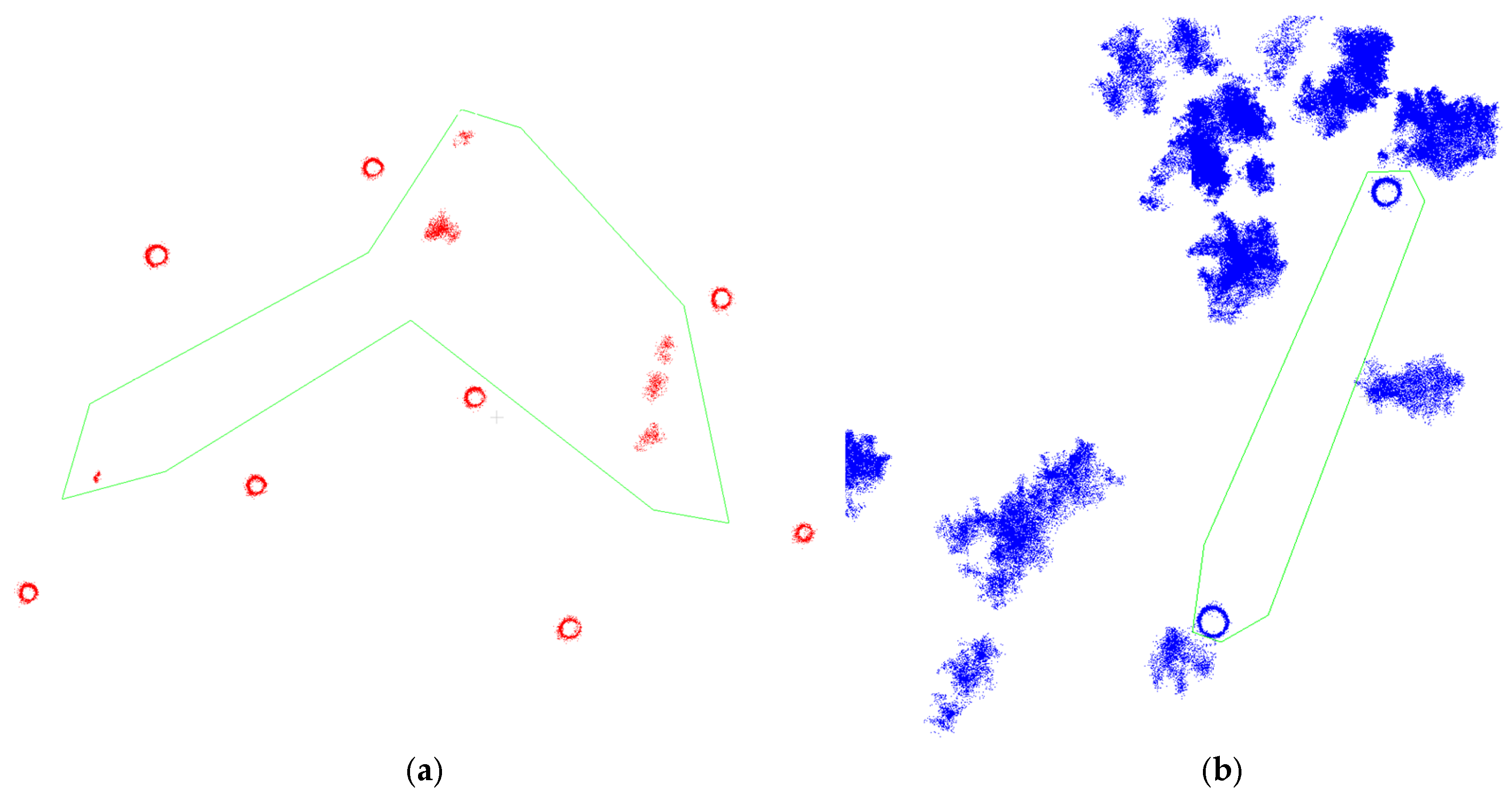
Figure 24 illustrates the procedure used to generate reference biometrics. The process begins with the isolation of a horizontal cross-section of the input point cloud at the standard breast height interval (normalized height between 1.3 m and 1.8 m), as shown in Figure 24a. This slice is then cropped using the same trajectory buffer principle described earlier, so that sparse trees far from the trajectory are excluded, as shown in Figure 24b, by using a distance buffer around the trajectory. To isolate potential stem candidates, the DBSCAN algorithm is applied to the sliced data. The resulting clusters are preliminarily categorized based on geometric extent; clusters with a 2D extent exceeding 1.5 m are flagged as outlier clusters, representing potential noise or undergrowth, while the remaining clusters are designated as initial stem clusters, as shown in Figure 24c.
Following the automated clustering, a manual quality control phase is conducted to ensure the integrity of the initial stem clusters. This refinement is performed via visual inspection and follows a two-step workflow. First, the initial stem clusters are reviewed to filter out noise points, resulting in a dataset of refined stems, as shown in Figure 25a. Simultaneously, the flagged outlier clusters are inspected to recover any valid stems that were incorrectly rejected by the geometric threshold, as shown in Figure 25b. A candidate is retained as a valid reference stem when a distinct stem cross-section can be visually identified in the original breast height slice and separated from surrounding vegetation or noise. Candidates that cannot be clearly associated with a stem are excluded.
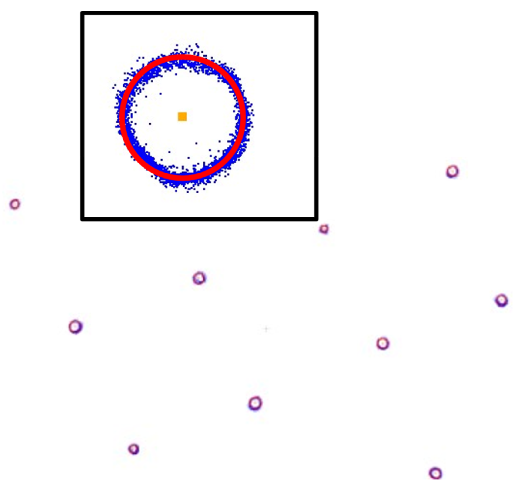
The primary objective of this stage is to generate a spatially accurate reference stem map for the quantitative assessment of the proposed method. To achieve this, the refined stems are merged with the manually recovered missing stems to form a complete reference dataset, as illustrated in Figure 26. During the previous visual inspection stage, multi-stemmed trees are identified and their stems are separated so that each valid stem is assigned an individual reference location. Following a final visual check against the raw slice data to ensure completeness, a circle fitting algorithm is applied to the points within each validated cluster. This calculation explicitly estimates the stem center coordinates (X, Y), which are used here as the reference tree location at 1.5 m height, as shown in Figure 27.
These point cloud-derived reference tree locations were used only for tree detection evaluation. The quantitative DBH evaluation was conducted separately using the field-measured DBH values available for the Martell–BackPack dataset.

5. Evaluation Criteria and Experimental Results

This section presents the evaluation criteria and experimental validation of the proposed pipeline across the datasets described in Section 3. This evaluation includes the parameter settings, evaluation metrics, tree detection results, qualitative assessment of individual tree segmentation, and derived biometrics evaluation.

5.1. Parameter Configuration

The proposed pipeline contains both globally fixed and acquisition modality-dependent parameters. One fixed parameter configuration was applied to all proximal datasets, including BackPack, ATV, and handheld acquisitions, regardless of the forest environment or sensor brand. A second configuration was applied to the UAV dataset to account for its lower point density, top–down viewing geometry, and reduced lower-stem visibility. No parameter adjustment was performed for individual forest environments within either acquisition modality. A complete list of these parameters is provided in Table A2.

5.2. Evaluation Metrics

The proposed pipeline was evaluated using the eight datasets described in Section 3, which encompass varying platforms (BackPack, ATV, Handheld, UAV), sensor specifications, and forest environments. Additionally, the method is benchmarked against the geometric algorithm 3DFIN and two state-of-the-art deep learning models: TreeLearn [22] and ForestFormer3D [21]. The benchmark methods were evaluated using their publicly available implementations. Table 2 summarizes their versions, input preprocessing, principal settings, and model adaptation status. 3DFIN was applied using its default parameter configuration for all datasets without dataset-specific tuning. TreeLearn and ForestFormer3D were evaluated using their publicly available pretrained models without fine-tuning on the study datasets. The input point clouds were prepared according to the preprocessing requirements of each implementation, and no dataset-specific adaptation was performed. Therefore, the deep learning results represent direct inference using pretrained models rather than performance after model adaptation to the evaluated datasets. No benchmark parameters were optimized or fine-tuned before conducting the evaluation of the study datasets. Therefore, the deep learning results represent direct inference using pretrained models rather than performance after model adaptation to the evaluated datasets. The performance of the pipeline on these datasets was assessed through experiments focused on tree detection, individual tree segmentation, and biometrics estimation.
Tree detection accuracy was quantitatively evaluated by matching the detected tree locations with the reference tree locations for each dataset. Detected and reference tree locations were matched based on their 2D Euclidean distance in the horizontal plane using a maximum matching distance of 0.25 m. Each reference tree was matched to only one detected tree. A matched pair was considered a TP, while unmatched detections and reference trees were counted as FP or FN, respectively. The same matching criterion was applied to all evaluated methods and datasets. Two reference data types were used in this study. Tree detection results for the Martell datasets were evaluated using independent field-measured tree locations, while DBH accuracy was evaluated using field measurements for correctly detected trees. The remaining datasets were evaluated using semi-automatically generated and manually refined reference data from the available point clouds. True positives (TPs) represent detected trees that correctly match reference trees, false positives (FPs) represent detected trees with no counterpart in the reference data, and false negatives (FNs) represent reference trees that were not detected. These counts were used to calculate Precision, Recall, and the F1-score (Equations (2)–(4)).
Individual tree segmentation refers to the assignment of point cloud points to separate tree instances after tree detection. Segmentation quality was assessed through qualitative comparisons of tree completeness, separation between neighboring trees, and representative over-segmentation and under-segmentation cases. Therefore, the reported Precision, Recall, and F1-score values quantify tree detection rather than point-level segmentation accuracy.
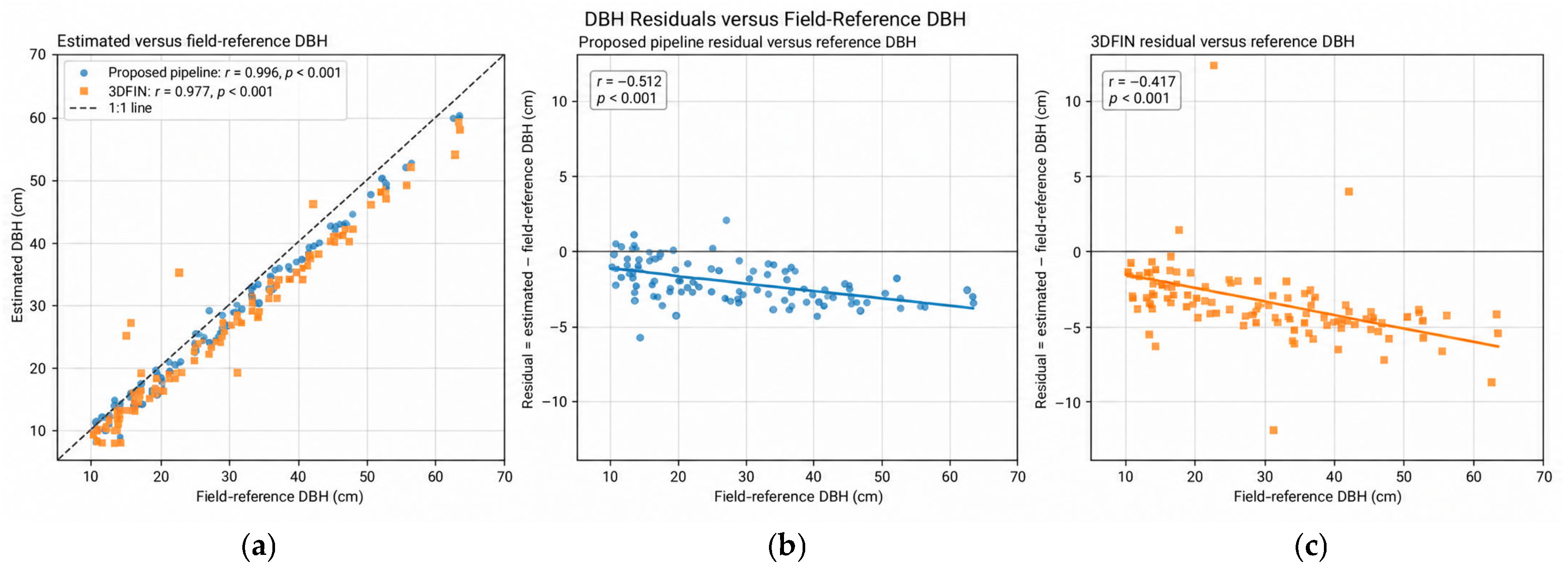
DBH accuracy was assessed only for the Martell–BackPack trees that were successfully detected by the pipeline and had corresponding field-measured values. Pearson’s correlation coefficient (r), its corresponding p-value, RMSE, and error statistics were reported for this tree-level comparison. To determine whether DBH errors were related to tree size, residuals were calculated as the difference between the estimated and field-measured DBH values. These residuals are then correlated with field-measured DBH values using Pearson’s correlation coefficient and the corresponding p-value for both the proposed pipeline and 3DFIN. Negative residuals indicate underestimation. Moreover, the statistically significant negative correlation between DBH residuals and field-measured DBH values indicates that the residuals depend on tree size, with larger trees showing greater underestimation. Since DBH error statistics do not account for trees that were missed during detection, an inventory-level basal area comparison was performed to account for the combined effects of missed trees, false detections, and DBH estimation errors.
P r e c i s i o n = T P T P + F P  
R e c a l l = T P T P + F N  
F 1 s c o r e = 2 P r e c i s i o n R e c a l l P r e c i s i o n + R e c a l l

5.3. Computational Efficiency

The proposed pipeline and 3DFIN were executed on a workstation equipped with an Intel Core i7-13700 processor, 32 GB of RAM, and an NVIDIA GeForce RTX 3070 GPU with 8 GB of memory. TreeLearn and ForestFormer3D were executed on a server equipped with two Intel Xeon Silver 4316 processors, 256 GB of RAM, and eight NVIDIA RTX A5000 GPUs with 24 GB of memory per GPU. Table 3 summarizes the input point count and total processing time for each dataset and method. Because the methods were executed on different hardware configurations, the reported runtimes provide an indication of computational requirements rather than a strictly controlled head-to-head efficiency comparison.
The proposed pipeline processed all datasets within 8–102 min, with the longest processing time observed for the Martell–BackPack dataset, which contained the largest number of points. Although processing time generally increased with dataset size, the results also indicate that runtime was affected by the processing strategy of each method. 3DFIN was faster for several proximal datasets, whereas ForestFormer3D generally required the longest processing time. Considering the different hardware configurations, these results demonstrate that the proposed pipeline provides practical processing times across datasets with different sizes and acquisition characteristics.

5.4. Comparative Results Across Study Sites

This section presents the experimental results of the proposed pipeline and benchmark methods across the evaluated datasets. The results are organized by forest condition and acquisition setting to highlight performance under different environments and platform characteristics.
Table 4 provides a compact summary of the quantitative tree detection results across all evaluated datasets and methods. The table distinguishes evaluations based on independent field measurements from those based on point cloud-derived reference data and reports the available biometric errors for the Martell–BackPack dataset. The following subsections provide qualitative comparisons and site-specific interpretations of the principal trends and failure cases.

5.5. Performance in Plantation Environments

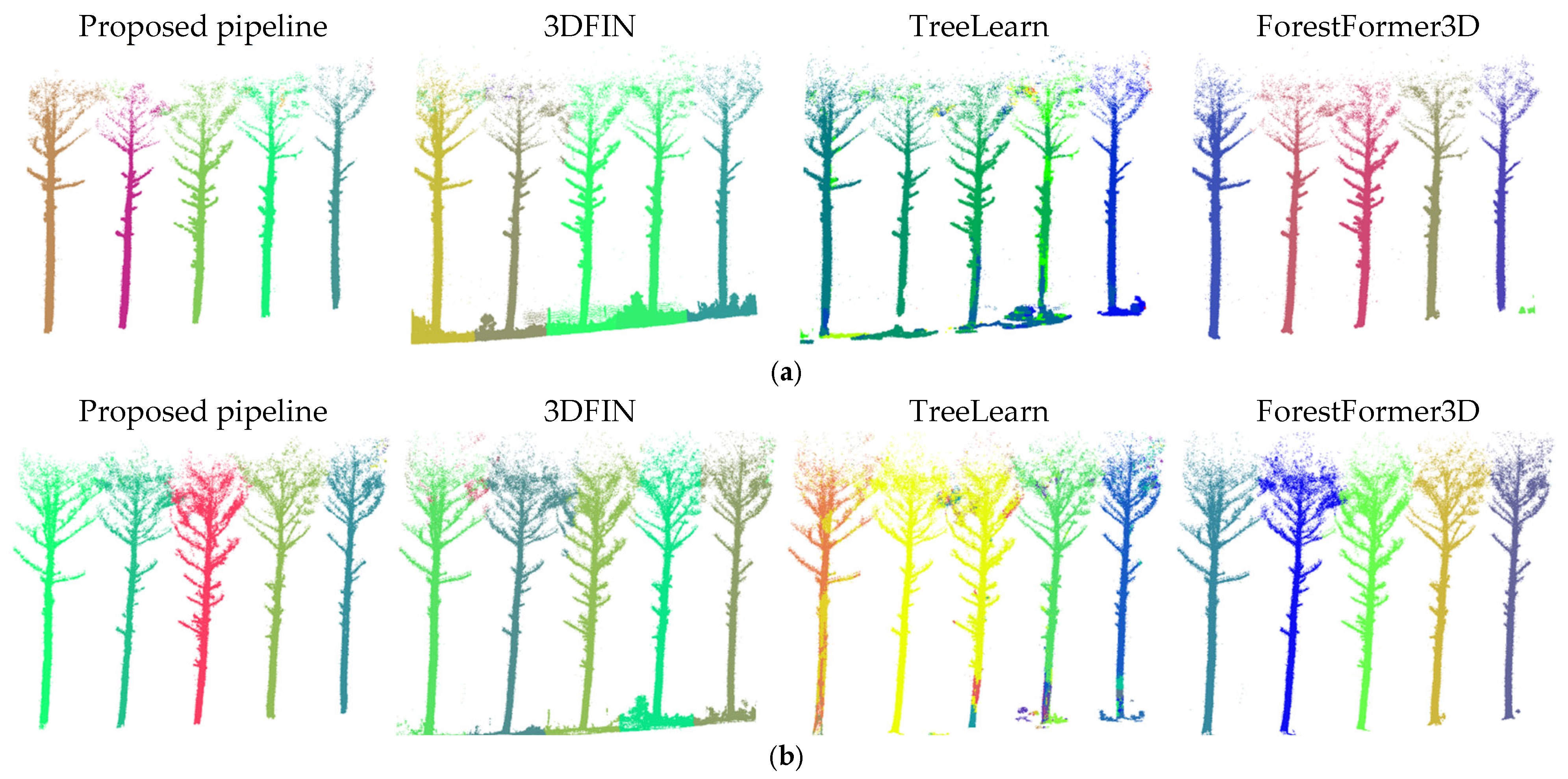
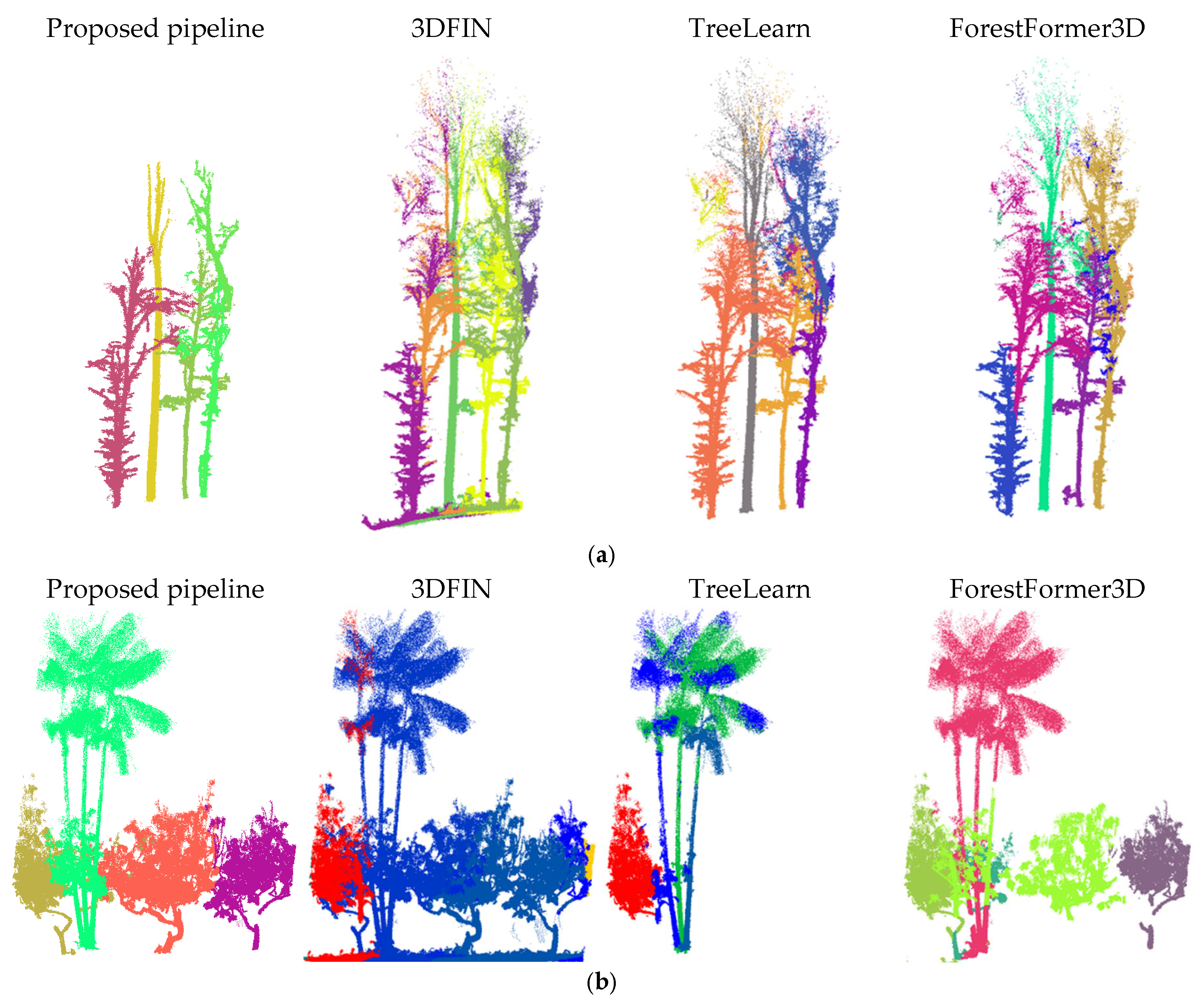
This test focuses on the Whitehall plantation datasets for validating the cross-platform robustness under controlled stand conditions. Whitehall plantation was captured with two platforms: a BackPack-Knap-XP1 and an ATV-Knap-XP1. Specifically, this comparison tests the pipeline’s robustness to varying point densities caused by distinct acquisition dynamics: the pedestrian-paced walking trajectory of the BackPack unit versus the higher-speed, vehicle-based trajectory of the ATV system. Figure 28 presents a qualitative comparison of the final segmentation results for the Whitehall–BackPack and Whitehall–ATV datasets across the proposed pipeline and the benchmark approaches. The plantation structure was generally well segmented by most methods, with clear separation between individual trees. However, TreeLearn produced several over-segmentation errors, where single trees were split into multiple segments.
Table 5 summarizes the tree detection performance for the Whitehall–BackPack and Whitehall–ATV datasets. Bold values indicate the highest Precision, Recall, and F1-score within each dataset The proposed pipeline achieved the highest overall performance, with an F1-score of 98.15% for the BackPack dataset and 100.00% for the ATV dataset. 3DFIN also performed well, but its F1-scores were slightly lower, particularly for the ATV dataset, where missed detections and false positives reduced its performance. TreeLearn showed the weakest performance, mainly because of the large number of false positives, which is consistent with the over-segmentation observed in Figure 28. ForestFormer3D achieved complete Recall on both datasets, but its lower Precision indicates that it also introduced extra detections. Overall, these results show that the proposed pipeline maintained stable performance across the two acquisition platforms while reducing both missed trees and false detections.

5.6. Performance in a Mixed-Species Natural Forest with Field Reference Data

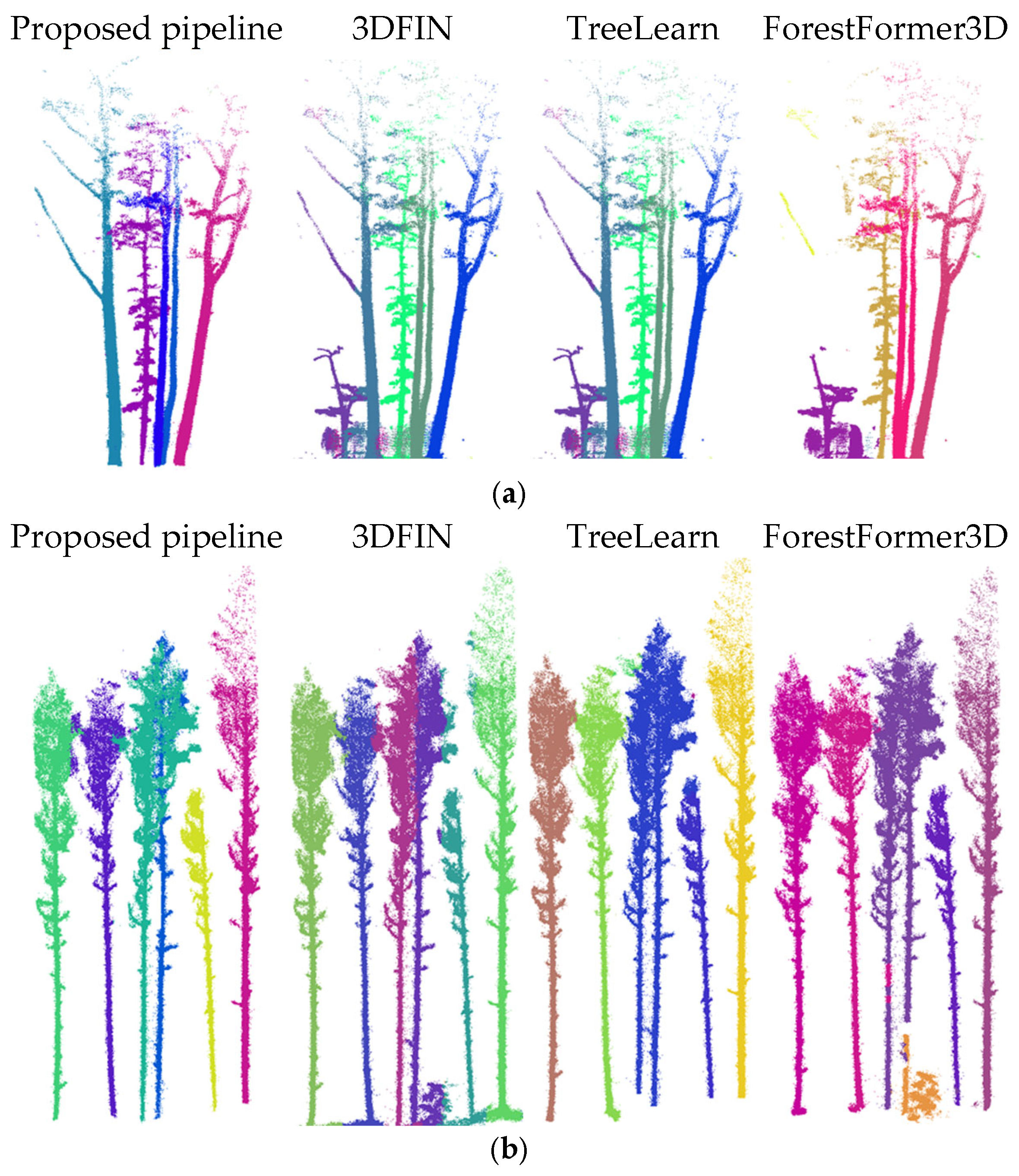
The Martell 4D site serves as the main benchmark for quantitative evaluation because it includes field reference measurements for both tree detection and DBH estimation. This subsection compares the proposed pipeline against benchmark approaches on both the Martell–BackPack and UAV datasets in order to assess performance under contrasting proximal and near-proximal acquisition conditions. Figure 29 presents a qualitative comparison of segmentation results across all tested methods. Overall, the qualitative results show that the proposed pipeline, 3DFIN, and TreeLearn produced more coherent segmentation outputs for the BackPack dataset, while TreeLearn and the proposed pipeline showed clearer tree separation in the UAV dataset. In contrast, ForestFormer3D produced poorer segmentation results in both acquisition settings, with several missed trees.
Table 6 reports the quantitative tree detection results for the Martell–BackPack and Martell–UAV datasets using the field reference data, where bold values indicate the highest Precision, Recall, and F1-score within each dataset For the Martell–BackPack dataset, the proposed pipeline achieved the highest F1-score of 97.25%, with a strong balance between PPrecision (97.55%) and RRecall (96.95%). This indicates that the pipeline was able to detect most reference trees while producing only a limited number of false positives. In comparison, 3DFIN and TreeLearn produced lower but still comparable F1-scores of 90.69% and 90.96%, respectively. Their performance was mainly limited by higher false positive counts, rather than missed detections. ForestFormer3D showed the weakest result on this dataset, with an F1-score of 44.39%, reflecting substantial segmentation errors under the mixed-species natural forest conditions.
For the Martell–UAV dataset, the results followed a different trend. TreeLearn achieved the highest F1-score of 91.80%, mainly due to its very high Precision. The proposed pipeline achieved an F1-score of 88.89%, with the same Recall as TreeLearn but lower Precision. This suggests that the proposed method remained effective on the UAV data, but the sparse lower-stem observations increased the number of false detections compared with TreeLearn. ForestFormer3D again showed lower performance, with an F1-score of 75.44%, mainly because of reduced Recall. The 3DFIN implementation failed to produce meaningful results for the UAV point cloud and was therefore excluded, likely because the UAV data did not provide a sufficiently continuous lower-stem structure for its stem-based processing. Overall, the results show that the proposed pipeline performed best on the proximal BackPack dataset and remained competitive on the near-proximal UAV dataset, while TreeLearn achieved the strongest result for the UAV case.
Table 7 summarizes the DBH estimation results for the proposed pipeline and 3DFIN. The comparison is limited to these two methods since 3DFIN was the only benchmark method that produced DBH estimates. The analysis considered correctly detected Martell–BackPack trees with corresponding field measurements. The DBH evaluation included 156 correctly detected trees with corresponding field measurement in the Martell–BackPack dataset. Based on the field-measured DBH values, the sample included 6 trees below 20 cm, 40 trees between 20 and 30 cm, 35 trees between 30 and 40 cm, and 75 trees with DBH ≥ 40 cm. Estimation performance was evaluated using error statistics, Pearson’s correlation coefficient, and the associated p-value. Figure 30a compares the estimated and field-measured DBH values, while Figure 30b,c show how the estimation residuals vary with tree size for the proposed pipeline and 3DFIN, respectively. Residuals were calculated as the difference between the estimated and field-measured DBH values, with negative values indicating underestimation.
Because the preceding tree-level DBH evaluation was restricted to correctly detected trees, an inventory-level basal area comparison was conducted to account for the combined effects of missed trees, false detections, and DBH estimation errors, as reported in Table 8. The field-reference basal area for the Martell–BackPack ROI was 11.17 m2. The proposed pipeline estimated 10.96 m2, corresponding to an underestimation of 0.21 m2 (1.88%), whereas 3DFIN estimated 10.76 m2, corresponding to an underestimation of 0.41 m2 (3.67%). Therefore, the proposed pipeline provided an inventory-level basal area estimate closer to the field reference.
The proposed pipeline achieved an RMSE of 2.5 cm and a strong positive relationship between the estimated and field-measured DBH values (r = 0.996, p < 0.001). In comparison, 3DFIN achieved an RMSE of 4.0 cm, with a correlation of r = 0.977 (p < 0.001). The residual analysis showed a statistically significant negative relationship between DBH residuals and field-reference DBH values for both the proposed pipeline (r = −0.512, p < 0.001) and 3DFIN (r = −0.417, p < 0.001). Thus, the residuals became increasingly negative as tree size increased, indicating that both methods tend to underestimate larger trees. This systematic trend may be partly explained by the difference between the field and LiDAR measurement principles. The field-measured DBH was derived from measurements of the stem’s outer circumference, including the outer bark, whereas the LiDAR-based DBH was estimated by fitting a circle to the visible points in the stem cross-section. When the outer stem surface is incompletely or unevenly sampled, the fitted circle may lie inside the actual outer stem boundary and consequently underestimate DBH. Although both methods exhibited this size-dependent trend, the proposed pipeline maintained the lower overall DBH estimation error. Representative stem cross-sections and fitted circles are shown in Figure 31.

5.7. Performance Under Sparse Single-Pass Trajectory Pattern and Dense Handheld Acquisition

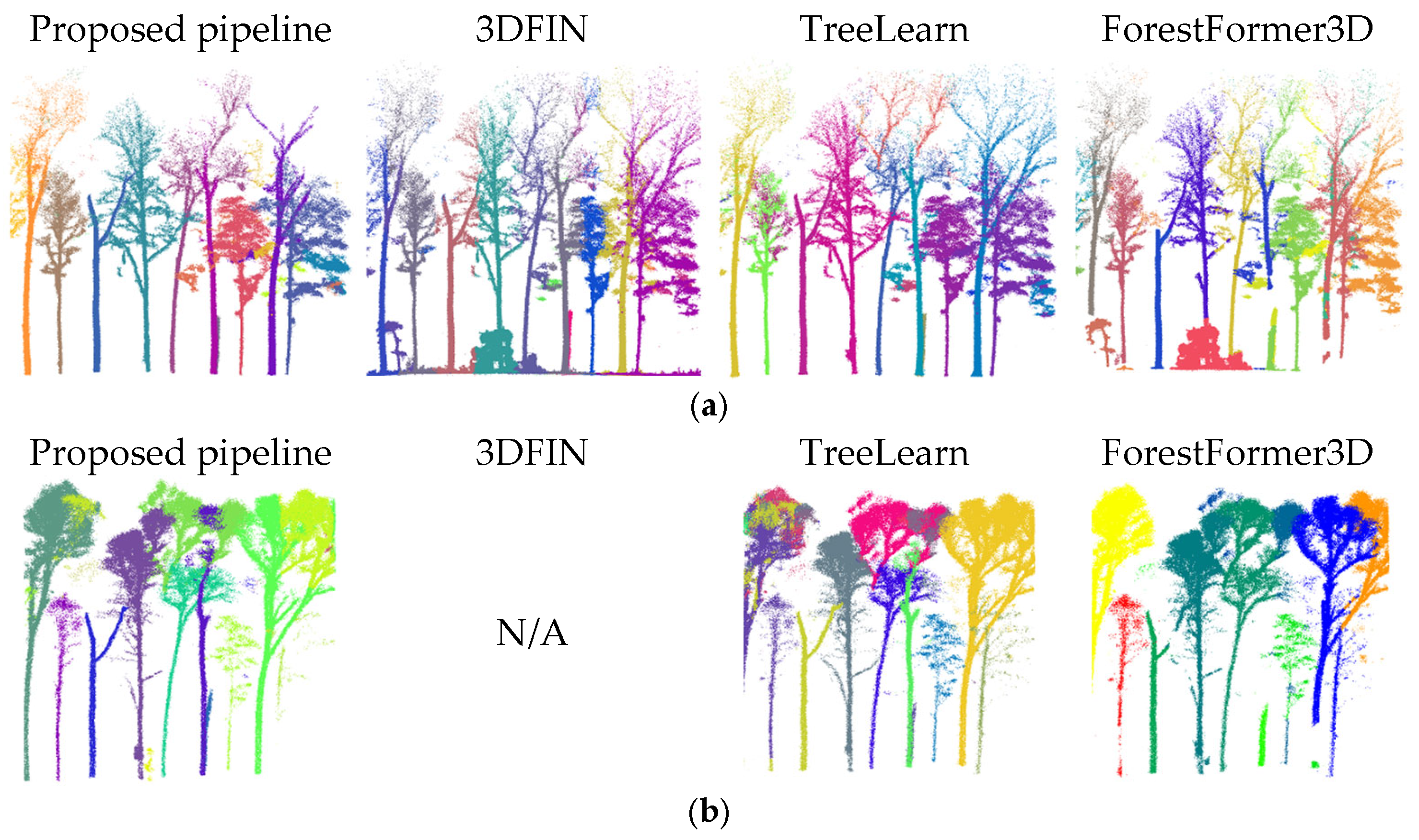
Two datasets were used to evaluate the proposed pipeline under contrasting point cloud sampling conditions. The Michigan–BackPack dataset represents a challenging single-pass trajectory scenario, where limited coverage and distance-dependent sparsity led to sparse stem sampling. In contrast, the NIBIO–Handheld dataset represents a dense boreal dataset acquired with a handheld MLS system, providing substantially higher and more continuous point coverage. Presenting these datasets together allows the pipeline to be assessed under two opposing acquisition conditions, from sparse and incomplete single-pass data to dense handheld LiDAR data. Figure 32 presents a qualitative comparison of segmentation results across all tested methods for the Michigan and NIBIO datasets.
Table 9 summarizes the tree detection results for both datasets. Within each dataset, bold values indicate the best performing method for Precision, Recall, and F1-score among the tested approaches. In the Michigan–BackPack dataset, all methods were challenged by the incomplete coverage associated with the single-pass trajectory. The proposed pipeline achieved an F1-score of 81.82%, which was slightly lower than that of 3DFIN (82.90%), but with substantially fewer false positives. By contrast, the slightly higher F1-score of 3DFIN was accompanied by lower Precision, indicating a greater tendency toward commission errors. TreeLearn showed lower overall performance, with a Recall of 76.92%, while ForestFormer3D performed worst, with Recall dropping to 60.98%. Overall, the proposed pipeline maintained the highest Precision and a better balance between omission and commission errors under these conditions.
In the NIBIO–Handheld dataset, the proposed pipeline achieved the highest F1-score (89.51%), outperforming 3DFIN (80.00%), TreeLearn (77.68%), and ForestFormer3D (84.44%). Its performance was supported by strong Recall (88.88%), indicating that the pipeline remained effective under dense boreal conditions.

5.8. Performance in Challenging Environments (Tropical and Dense Understory)

Two datasets were used to evaluate the proposed pipeline under particularly challenging forest conditions. The SEPAC–BackPack dataset represents a dense-understory temperate forest, where stem detection is complicated by irregular spacing and abundant understory vegetation. In contrast, the Brazil–BackPack dataset represents a tropical agroforestry environment with a multi-layered canopy and dense vegetation, making the separation of smaller trees from surrounding vegetation especially difficult. Figure 33 presents a qualitative comparison of segmentation results across all tested methods for the SEPAC–BackPack and Brazil–BackPack datasets. For the Brazil–BackPack dataset, the optional 3D U-Net understory removal module was disabled because small-diameter Açaí trees were valid inventory targets and could be classified as understory according to the model’s original DBH-based training definition. The effect of enabling this module is quantitatively evaluated in Section 5.9.
Table 10 summarizes the tree detection results for both datasets. Within each dataset, bold values indicate the best performing method for Precision, Recall, and F1-score among the tested approaches. In the dense-understory SEPAC–BackPack dataset, the proposed pipeline achieved an F1-score of 87.18%, with Precision and Recall of 86.44% and 87.93%, respectively, outperforming 3DFIN (69.33%), TreeLearn (82.35%), and ForestFormer3D (63.29%). In the Brazil–BackPack dataset, the proposed pipeline achieved an F1-score of 88.26%, successfully identifying 109 trees. By comparison, the competing methods showed substantially lower Recall values of 42.62% for 3DFIN, 32.78% for TreeLearn, and 40.16% for ForestFormer3D, indicating that many trees were missed under these tropical conditions. Overall, these results indicate that the proposed pipeline remained effective in both dense-understory temperate forest and tropical conditions. The SEPAC results show that the method retained a good balance between omission and commission errors in cluttered understory conditions, while the Brazil results highlight its ability to preserve smaller valid trees even without the optional understory removal module.

5.9. Ablation of the Optional Understory Removal Module

To quantify the contribution of the optional understory removal step, the complete pipeline was executed with and without this module for the Martell–BackPack and Brazil–BackPack datasets, while all remaining processing stages and parameters were kept unchanged, as presented in Table A2. The same forestry-adapted 3D U-Net was used without dataset-specific retraining. Martell–BackPack represents a natural forest in which dense low vegetation can generate false stem candidates, whereas Brazil–BackPack contains small valid Açaí trees that may exhibit structural characteristics similar to understory vegetation, as reported in Table 11.
For the Martell–BackPack dataset, disabling understory removal increased the number of false positives from 4 to 77 and reduced the F1-score from 97.25% to 75.45%. In contrast, enabling the module for the Brazil–BackPack dataset reduced the number of true positives from 109 to 15 and increased the number of false negatives from 13 to 107, resulting in an F1-score reduction from 88.26% to 18.87%. Visual inspection indicated that many valid small Açaí trees were classified as understory and removed.
These contrasting results confirm that the module is condition-dependent rather than universally beneficial. It is appropriate when the inventory targets larger or merchantable stems and small woody vegetation represents an unwanted source of false detections. It should be disabled or retrained with task-specific labels when trees below approximately 12 cm DBH are valid inventory targets. The selection is therefore based on the inventory objective and vegetation composition rather than a universal understory density or tree height threshold.

5.10. Error Analysis Based on Tree and Acquisition Conditions

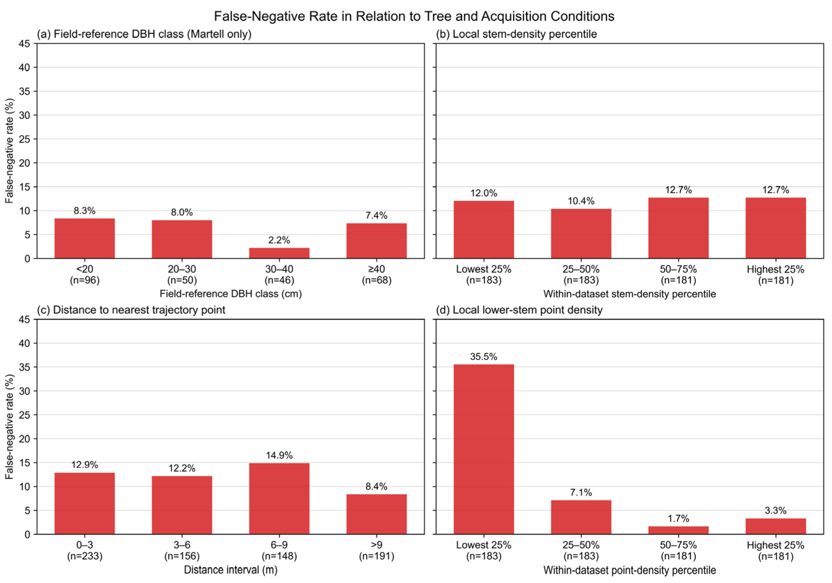
To further investigate the conditions associated with missed tree detections, the false negative rate was analyzed in relation to tree size, local stem density, distance from the acquisition trajectory, and local lower-stem point density. Tree size analysis was limited to the Martell datasets because independent field-reference DBH measurements were available only for this site. The reference trees were grouped into four DBH classes: less than 20 cm, 20–30 cm, 30–40 cm, and at least 40 cm. Local stem density was calculated as the number of neighboring reference stems within a 5 m radius and was expressed using within-dataset quartiles. For each reference tree, the horizontal distance to the nearest trajectory point was also calculated. Local lower-stem point density was determined from points within a horizontal radius of 0.5 m and a normalized height interval of 0.5–5 m around each reference stem. Stem density and point density percentiles were calculated independently within each dataset to account for differences among forest conditions and acquisition systems. The false negative rate for each group was calculated as the number of missed reference trees divided by the total number of reference trees in that group.
Figure 34 compares the false negative rate across four tree- and acquisition-related factors. Tree size did not show a consistent relationship with missed detections. For the Martell field-reference trees, the false negative rates were 8.3%, 8.0%, 2.2%, and 7.4% for the four DBH classes. The lower rate observed for the 30–40 cm class was not sustained in the largest DBH class, indicating that DBH alone was not a consistent predictor of detection success. Local stem density also showed limited variation in detection performance. The false negative rates were 12.0%, 10.4%, 12.7%, and 12.7% from the lowest to the highest stem density quartile. Therefore, increasing local stem density did not produce a clear monotonic increase in missed detections across the evaluated datasets. Similarly, the false negative rate did not exhibit a consistent monotonic relationship with distance from the acquisition trajectory. The rates were 12.9%, 12.2%, 14.9%, and 8.4% for the different distance intervals. This indicates that trajectory distance alone did not adequately explain missed detections. In contrast, local lower-stem point density showed a substantially clearer relationship with tree detection performance. The false negative rate was 35.5% in the lowest point density quartile and decreased to 7.1%, 1.7%, and 3.3% in the remaining quartiles. These results indicate that adequate sampling of the lower stem is more directly associated with successful detection than tree size, local stem density, or trajectory distance alone.

5.11. Tiling Sensitivity Analysis

A sensitivity analysis was conducted to evaluate the influence of tile size and overlap buffer on computational efficiency and tree detection consistency for the Martell–BackPack dataset. The full ROI was processed using each tiling configuration, while a fixed 30 × 30 m evaluation window within the ROI was used to compare the resulting tree detections. This window was used only for evaluation and was not the area being tiled. All tested configurations detected the same 59 trees within this evaluation window. The number of processed point records and processing time varied according to tile and overlap buffer size, as reported in Table 12. For a fixed tile size of 50 m, increasing the buffer from 2.5 to 7.5 m increased the processed point records from 112.7 million to 156.4 million and the processing time from 26.07 to 39.71 min.

6. Discussion

The experimental results across the evaluated datasets indicate that the proposed pipeline can provide accurate and reliable individual tree detection and segmentation under the tested forest structures, platforms, and acquisition systems. Relative to 3DFIN, TreeLearn, and ForestFormer3D, the method generally maintained a better balance between false positives and false negatives, suggesting that the confidence-guided quality control strategy helps reduce common failure modes such as spurious detections from understory shrubs, missed stems, under-segmentation, and over-segmentation in cluttered stands. The evaluation across these contrasting ROI-level datasets demonstrates the behavior of the proposed workflow under different platform, sensors, trajectory, and forest structure conditions; however, it should be interpreted as a multi-case technical evaluation rather than evidence of universal environmental transferability. The results should also be interpreted according to the scope of each evaluation. Tree detection has the broadest quantitative assessment, with Precision, Recall, and F1-score reported across all eight datasets. Individual tree segmentation was assessed qualitatively through tree completeness, separation between neighboring trees, and representative over- and under-segmentation cases. Biometric extraction was quantitatively evaluated using field-measured DBH and inventory-level basal area for the Martell–BackPack dataset. Therefore, the quality of DBH and basal area results, as well as tree detection for the Martell–BackPack dataset, has been validated by field-based reference data. On the other hand, the tree detection performance of the proposed pipeline for the remaining datasets has been evaluated using semi-automatically generated, manually refined reference data from the same point clouds.
However, since the reference data have been generated from the same point cloud processed by the proposed approach, such data may favor trees that are clearly represented in the data and should not be considered equivalent to independent field validation. Independent field-reference measurements were available only for the Martell site, while the remaining datasets relied on reference data derived from the point cloud processed by the proposed approach. Future work should therefore extend the evaluation using independent field measurements across additional forest environments and acquisition platforms.
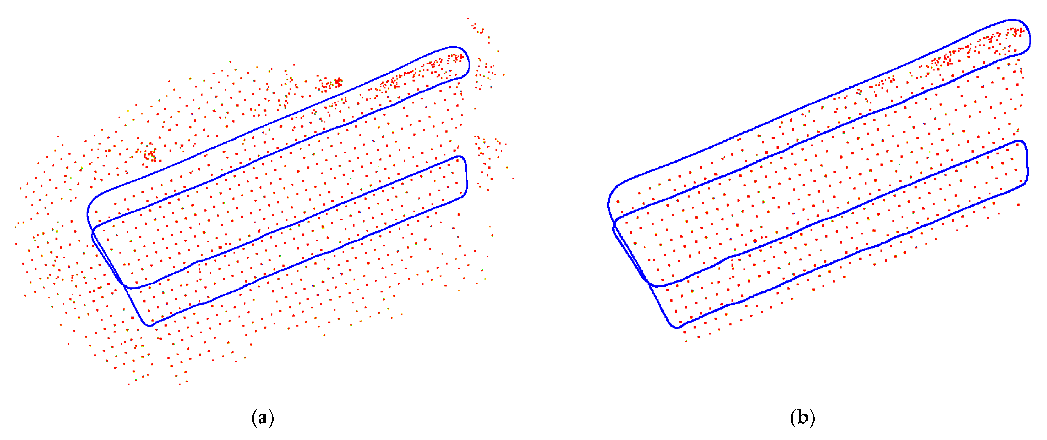
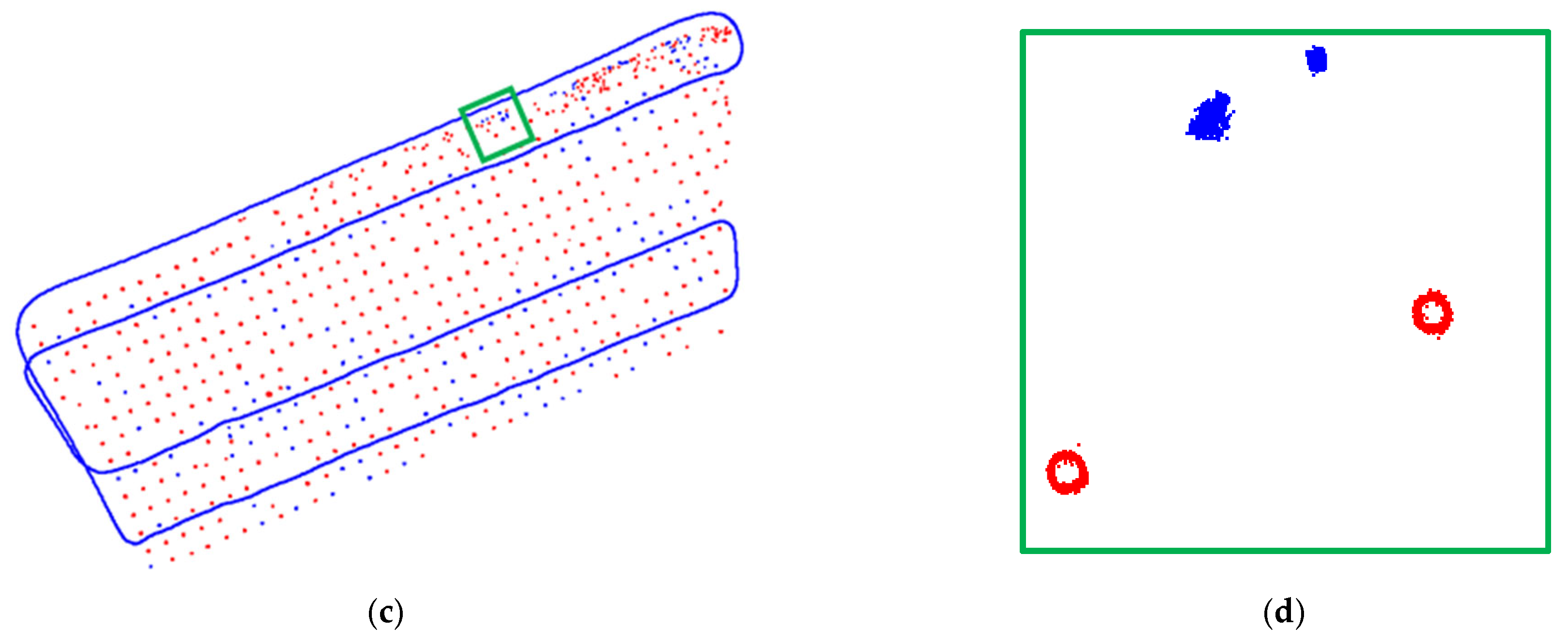
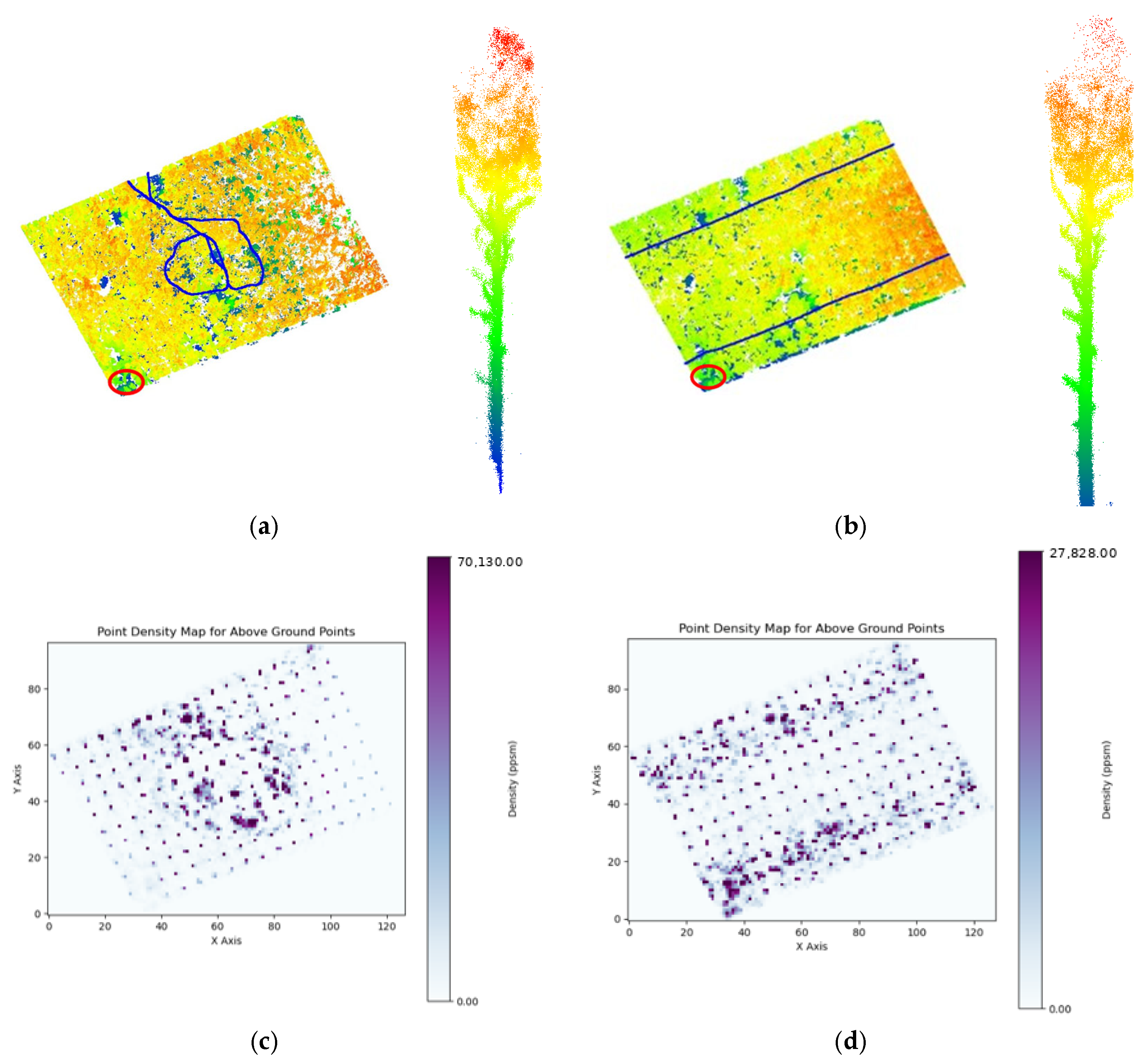
The Whitehall plantation experiments provide the clearest assessment of cross-platform robustness under relatively controlled stand conditions. The proposed pipeline achieved near-perfect detection on both Whitehall datasets. However, one tree was missed in the BackPack dataset. This omission appears to be related to overall point density and coverage reduction near the ROI boundary. In the BackPack acquisition, the walking trajectory and turning behavior produced a locally sparse region near the plot edge, reducing the continuity of stem evidence available to the filtering and stem validation stages. In contrast, the ATV acquisition produced more uniform coverage along the stand boundaries and resulted in complete detection. This interpretation is supported by the trajectory visualization and above-ground point density maps in Figure 35, where the missed tree coincides with a localized low-density region at the ROI border. These results emphasize that trajectory design directly influences boundary tree completeness.
Beyond plantation conditions, the Martell 4D experiments further support the robustness of the proposed pipeline across contrasting acquisition platforms, including proximal BackPack data and near-proximal UAV data. On the BackPack dataset, the proposed pipeline achieved the highest overall F1-score among the tested methods and also produced the most accurate DBH estimates. Across the temperate natural forest datasets, particularly Martell 4D and SEPAC sites, the benchmark methods more often exhibited the familiar trade-off between merging neighboring trees and generating excess false positives from cluttered woody structures and understory vegetation. By contrast, the proposed pipeline maintained a better balance between omission and commission errors, consistent with the qualitative comparisons and FP/FN examples presented in Section 5.5, Section 5.6, Section 5.7, and Section 5.8.
The DBH residual analysis demonstrated a statistically significant size-dependent underestimation for both the proposed pipeline and 3DFIN. This pattern can partly be explained by the difference between the field and point cloud measurement principles. Field-reference DBH represents the outer circumference of the stem, including the outer bark, whereas point cloud DBH is estimated by fitting a circle to the visible stem points. LiDAR observations may represent only part of the outer stem surface because of occlusion, scanning geometry, understory vegetation, or irregular stem structure. Under these conditions, the fitted circle may lie within the actual outer stem boundary, producing increasingly negative residuals for larger trees. Representative regular and irregular cross-sections shown in Figure 31 illustrate this geometric effect. The residual analysis quantitatively confirms the relationship with tree size, while multi-stem structure and local understory are interpreted as possible contributing factors rather than independently verified causes. The DBH error analysis was not separately stratified by tree species or stem visibility conditions. Differences in stem geometry among species and variations in the completeness of the observed stem cross-section may influence circle fitting accuracy. Future field-based evaluation should therefore include species information and explicit stem visibility or occlusion classes to quantify their effects on DBH estimation.
The tropical and boreal case studies, Brazil–BackPack and NIBIO–Handheld, further evaluate the pipeline under canopy structures and visibility conditions that differ substantially from the temperate sites. Within these two test cases, the proposed pipeline outperformed the benchmark approaches, indicating that its core processing stages remained effective under the tested multi-layered tropical agroforestry and dense boreal conditions.
However, the remaining false negatives in heavily occluded areas highlight a practical limitation common to near-proximal LiDAR acquisitions. When the lower stem and understory are insufficiently observed, missing structural information cannot be reliably recovered through post-processing.
The understory removal ablation further demonstrates that this learned module should be treated as an optional, inventory-dependent component. Disabling the module for the Martell–BackPack dataset increased false positives from 4 to 77 and reduced the F1-score from 97.25% to 75.45%. In contrast, enabling it for the Brazil–BackPack dataset reduced the F1-score from 88.26% to 18.87% by removing many valid small Açaí trees. These contrasting results are consistent with the model’s original DBH-based training definition and indicate that the module is appropriate when larger or merchantable stems are the inventory objective, but should be disabled or retrained when small-diameter trees constitute valid inventory targets.
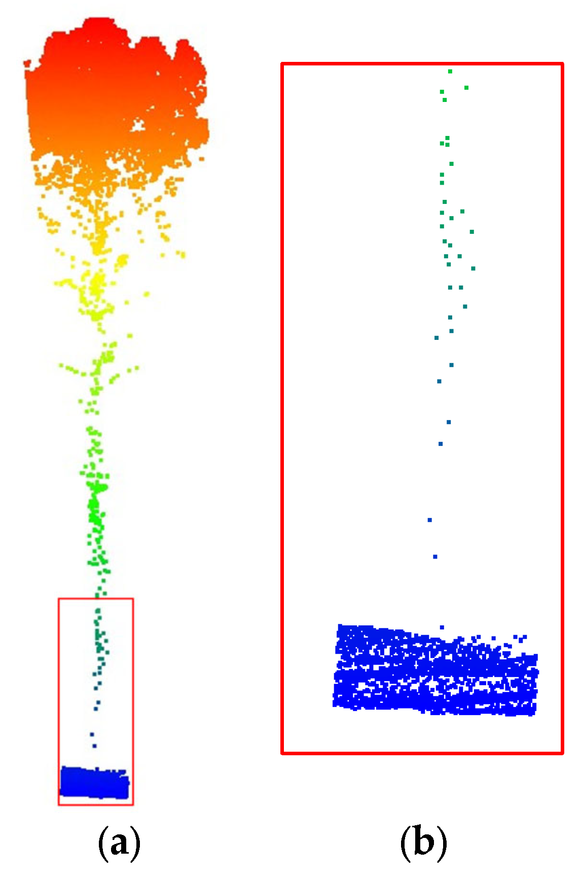
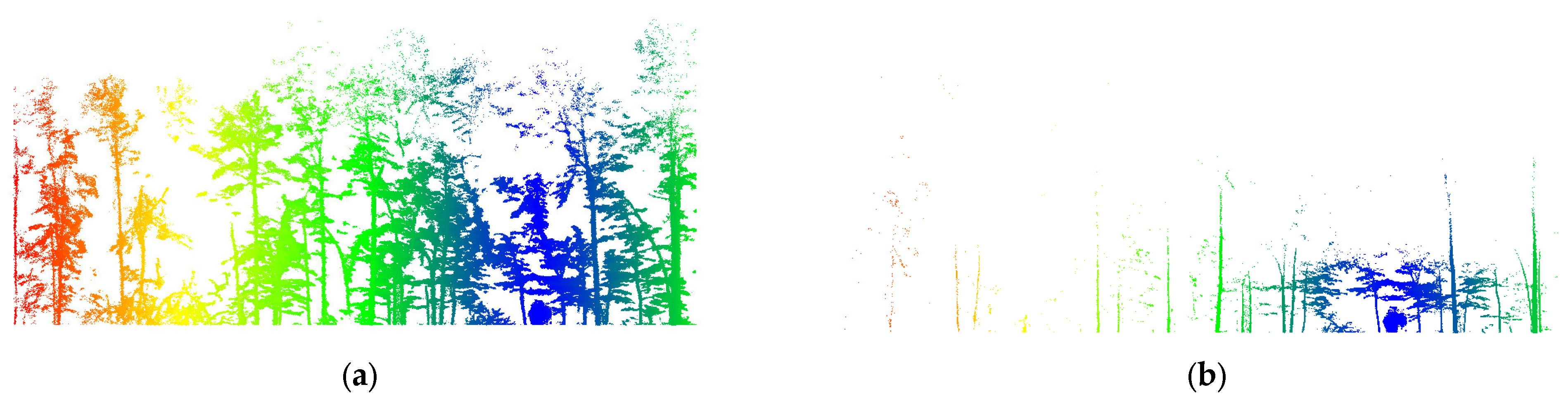
A related modality-specific effect is apparent in the UAV component of the Martell experiments, where reduced Recall is influenced by the trunk continuity check. While this module is effective for suppressing false positives from understory in proximal scans, it can become overly restrictive for top–down aerial data because UAV laser pulses are frequently occluded by the upper canopy, producing discontinuities and gaps in the lower-stem observations, as shown in Figure 36. This behavior highlights an important design trade-off: rules that improve Precision for cluttered ground-based scans may need to be relaxed or made view-adaptive for aerial acquisitions to avoid rejecting valid but fragmented stems.
Finally, the Michigan dataset highlights a limitation associated more with trajectory geometry than with forest type. In this dataset, the straight-line acquisition produces distance-dependent sparsity, so stems farther from the trajectory are sampled with lower point density [33]. These sparse observations are more vulnerable to removal during the filtering stage (Section 4.2), which prioritizes strong woody signatures, and valid but weakly represented stems may therefore be discarded as noise, as illustrated in Figure 37. In contrast, TreeLearn relies more heavily on learned semantic cues and can therefore retain valid stem hypotheses even under sparse observations, while 3DFIN achieved higher Recall by operating directly on the original point cloud without the same filtering constraints. From a practical perspective, these results show that acquisition design can be as important as algorithm choice. Integrating scan-planning strategies and online path tracking to maintain more uniform coverage could reduce distance-driven sparsity and improve segmentation completeness [34]. The expanded error analysis indicates that local lower-stem point density was the factor most clearly associated with missed detections. Tree size, local stem density, and distance from the trajectory did not exhibit consistent monotonic relationships with the false negative rate. This does not imply that these factors have no influence; rather, their effects are mediated by acquisition geometry, occlusions, trajectory overlap, vegetation structure, and line-of-sight conditions. For example, a tree located farther from the trajectory may still receive sufficient lower-stem observations, whereas a nearby tree may remain poorly sampled because of surrounding vegetation. Similarly, densely spaced trees do not necessarily lead to missed detections when their lower stems remain sufficiently visible. The false negative rate of 35.5% in the lowest point density quartile, compared with 1.7–3.3% in the upper two quartiles, demonstrates that the proposed bottom–up detection strategy primarily depends on the adequate local coverage of the lower stem.

7. Conclusions and Recommendations for Future Work

This study introduced a forest inventory pipeline evaluated across eight datasets captured using different sensors, platforms, acquisition patterns, and forest conditions, with parameter configurations fixed within each acquisition system. The proposed pipeline maintained strong and generally consistent tree detection performance across the evaluated cases, although it was not the highest performing method in every dataset. It achieved near-perfect F1-scores for the Whitehall plantation datasets, 97.25% for the Martell–BackPack dataset, 89.51% for the NIBIO–Handheld dataset, 87.18% for the SEPAC–BackPack dataset, and 88.26% for the Brazil–BackPack dataset. TreeLearn achieved the highest F1-score for the Martell–UAV dataset, while 3DFIN slightly exceeded the proposed pipeline for the Michigan–BackPack dataset.
The confidence-guided quality control strategy reduced common errors associated with false detections, merged clusters, multi-stem structures, and duplicated boundary trees. Tree detection received the broadest quantitative evaluation, while individual tree segmentation was assessed qualitatively. Field-based biometric validation was conducted for Martell–BackPack, where the proposed pipeline achieved a DBH RMSE of 2.5 cm and underestimated total basal area by 1.88%, compared with an RMSE of 4.0 cm and a basal area underestimation of 3.67% for 3DFIN. The remaining case studies were evaluated using point cloud-derived references and should therefore be interpreted as multi-case technical evaluations rather than independent field validation.
The results also identify important operational limitations. Reliable tree detection depends on sufficient lower-stem sampling, with a false negative rate of 35.5% observed in the lowest point density quartile. In addition, the optional understory removal module was beneficial for the Martell–BackPack dataset but removed many valid small Açaí trees in the Brazil dataset, confirming that its use should depend on the inventory objective and vegetation structure. Future work will focus on integrating top–down evidence, adaptive continuity criteria, and improved scan-planning strategies to mitigate sparse, occluded, or closely spaced tree trunks.
Furthermore, the pipeline’s reliance on automated intensity thresholding to isolate woody parts presents a challenge in sparse data scenarios. As observed in the Michigan dataset, trees located far from the sensor trajectory exhibit lower point density, which can cause the filtering module to misidentify valid stem points as noise and remove them, thereby reducing Recall. Future work should focus on mitigating these bottom–up dependencies by integrating “top–down” information, such as a parallel CHM detection method. Fusing the results from both approaches could create an even more robust consensus. Additionally, under-segmentation can still occur in cases of extreme proximity, such as when fallen trees lean against live stems or when multiple trunks are physically touching. Future research will address these spatial relationships. In addition, integrating optimal scan planning is expected to improve scan overlap, reduce distance-driven sparsity, and increase segmentation completeness in operational deployments. Finally, these individually segmented point clouds can be used for tree species identification by using their detailed geometric features. Moreover, the pipeline’s output is ideal for detailed stem reconstruction, which will enable the precise estimation of merchantable volume.

Author Contributions

Conceptualization, H.H., S.F. and A.H.; methodology, H.H., S.P. and A.H.; software, H.H. and S.P.; validation, H.H., S.P. and A.H.; writing—original draft preparation, H.H.; writing—review and editing, H.H., S.P., S.F. and A.H.; supervision, S.F. and A.H. All authors have read and agreed to the published version of the manuscript.

Funding

The authors acknowledge funding support from the PERSEUS grant, #2023-68012-38992, USDA NIFA USDA Awards, #2024-67021-42879 and NSF Award 2411273.

Data Availability Statement

The raw data supporting the conclusions of this article will be made available by the authors on request.

Conflicts of Interest

The authors declare no conflicts of interest.

Appendix A

Table A1. BackPack specifications.
SystemE2HDL32EKnap-XP1
LiDAR Specifications
Number of laser beams3264
Horizontal FOV360°360°
Vertical FOV (angle range from sensor’s horizon)41.33°
(−30.76° to +10.67°)
42.4°
(−22.5° to +22.5°)
Pulse per second~695,000~1,310,000
GNSS/INS Specifications
IMU data rate200 Hz200 Hz
Positional accuracy *1–2 cm1–2 cm
Attitude accuracy (roll/pitch) *0.005°0.1°
Attitude accuracy (heading) *0.010°0.5°
* After GNSS/INS post-processing in open-sky conditions.
The parameter values were selected by considering tree spacing, stem dimensions, and point cloud sampling density rather than by optimizing them separately for each dataset. For example, a minimum distinguishable stem-axis spacing of approximately 0.25 m was assumed for closely spaced trees. Accordingly, the DBSCAN neighborhood radius was selected to be smaller than this spacing so that points from adjacent stems were less likely to be connected within the same cluster. Parameters related to RANSAC circle fitting were defined according to the expected range of forest stem radii while the minimum point support is chosen to form a reliable cross-section. Similarly, vertical-layer and continuity parameters were selected according to the expected representation of the lower stem and difference in sampling density between proximal and UAV acquisitions. These values were kept fixed across forest environments within each acquisition system. The system-dependent configuration was changed to account for the substantially lower point density and top–down viewing geometry of the UAV data. Table A2 summarizes the parameter categories, values, physical rationale, and conditions under which adjustment may be required for new datasets.
Table A2. Parameters and threshold values used in experimental results.
VariableDescriptionThreshold/ParameterParameter Tuning
BackPackUAV
TbBuffer distance around the trajectory used to define the ROI25 mFixed
OdTile overlap distance5 mFixed
I f Otsu’s intensity filtering thresholdAutomatically derived
P l , P w , P h Prism dimensions for eigenvalue calculation0.5 × 0.5 × 4 mFixed
L t h Linearity threshold value for geometry filtering0.5Fixed
N p SOR number of nearest neighbors considered for distance calculation at each point100Fixed
α SOR multiplication factor for outlier removal2Fixed
ε DBSCAN neighborhood radius used for initial stem clustering0.2 mFixed
MinPtsMinimum number of points for DBSCAN grouping205Modality dependent
N s Number of sections along the tree trunk used for continuity check4Fixed
C s Grid cell size for sum of elevation approach0.1 mFixed
C h Minimum cluster height threshold3 m1 mModality dependent
P n Minimum number of points inside a section for trunk continuity check5Fixed
E r Tree trunk empty sections ratio to total sections25%Fixed
H m i n Min height used to isolate the normalized point cloud0.5 mFixed
H m a x Max height used to isolate the normalized point cloud5 mFixed
S d Number of slices used for RANSAC-based-tree detection4Fixed
T c Threshold used to filter cross-sections based on radius<5 cm or >80 cmFixed
T f Threshold for fitted circle RMSE for accepted sections0.1 mFixed
C p Cross-section completeness percentage for accepted cross-sections50%Fixed
S c Number of slices used for tree trunk cleaning10Fixed
R c Threshold used to assess the consistency for cross-section radii0.2 mFixed
V d Size used to voxelize point cloud before filtered points retrieval0.4 mFixed
R i Radius used for retrieving filtered points0.4 mFixed
I Number of iterations for filtered point retrieval1Fixed
T b s Buffer size for removing trees at tile boundaries5 mFixed
E Tree 2D extent used to identify abnormal tree clusters during point retrieval15 mFixed

References

  1. White, J.C.; Coops, N.C.; Wulder, M.A.; Vastaranta, M.; Hilker, T.; Tompalski, P. Remote sensing technologies for enhancing forest inventories: A review. Can. J. Remote Sens. 2016, 42, 619–641. [Google Scholar] [CrossRef] [Scilit]
  2. Weiser, H.; Schäfer, J.; Winiwarter, L.; Krašovec, N.; Fassnacht, F.E.; Höfle, B. Individual tree point clouds and tree measurements from multi-platform laser scanning in German forests. Earth Syst. Sci. Data 2022, 14, 2989–3012. [Google Scholar] [CrossRef] [Scilit]
  3. Fassnacht, F.E.; White, J.C.; Wulder, M.A.; Næsset, E. Remote sensing in forestry: Current challenges, considerations and directions. Forestry 2024, 97, 11–37. [Google Scholar] [CrossRef] [Scilit]
  4. Holvoet, J.; Eichhorn, M.P.; Giannetti, F.; Kükenbrink, D.; Liang, X.; Mokroš, M.; Novotný, J.; Pitkänen, T.P.; Puliti, S.; Skudnik, M.; et al. Terrestrial and mobile laser scanning for national forest inventories: From theory to implementation. Remote Sens. Environ. 2025, 329, 114947. [Google Scholar] [CrossRef] [Scilit]
  5. Wielgosz, M.; Puliti, S.; Xiang, B.; Schindler, K.; Astrup, R. SegmentAnyTree: A sensor and platform agnostic deep learning model for tree segmentation using laser scanning data. Remote Sens. Environ. 2024, 313, 114367. [Google Scholar] [CrossRef] [Scilit]
  6. Dalla Corte, A.P.; Souza, D.V.; Rex, F.E.; Sanquetta, C.R.; Mohan, M.; Silva, C.A.; Zambrano, A.A.; Prata, G.; de Almeida, D.R.A.; Trautenmüller, J.W.; et al. Forest inventory with high-density UAV-Lidar: Machine learning approaches for predicting individual tree attributes. Comput. Electron. Agric. 2020, 179, 105815. [Google Scholar] [CrossRef] [Scilit]
  7. Xiang, B.; Wielgosz, M.; Kontogianni, T.; Peters, T.; Puliti, S.; Astrup, R.; Schindler, K. Automated forest inventory: Analysis of high-density airborne LiDAR point clouds with 3D deep learning. Remote Sens. Environ. 2024, 305, 114078. [Google Scholar] [CrossRef] [Scilit]
  8. Calders, K.; Adams, J.; Armston, J.; Bartholomeus, H.; Bauwens, S.; Bentley, L.P.; Chave, J.; Danson, F.M.; Demol, M.; Disney, M.; et al. Terrestrial laser scanning in forest ecology: Expanding the horizon. Remote Sens. Environ. 2020, 251, 112102. [Google Scholar] [CrossRef] [Scilit]
  9. Castanheiro, L.F.; Campos, M.B.; da Silva, M.F.; da Silva, R.M.; dos Santos, R.C.; Galo, M.; Tommaselli, A.M.G. Assessment of tree detection and segmentation pipelines for terrestrial laser scanning dataset of orange orchards. Int. Arch. Photogramm. Remote Sens. Spat. Inf. Sci. 2025, XLVIII-2/W11-2025, 39–46. [Google Scholar] [CrossRef] [Scilit]
  10. Pu, Y.; Xu, D.; Wang, H.; Li, X.; Xu, X. A new strategy for individual tree detection and segmentation from leaf-on and leaf-off UAV-LiDAR point clouds based on automatic detection of seed points. Remote Sens. 2023, 15, 1619. [Google Scholar] [CrossRef] [Scilit]
  11. Nemmaoui, A.; Aguilar, F.J.; Aguilar, M.A. Benchmarking of individual tree segmentation methods in Mediterranean forest based on point clouds from unmanned aerial vehicle imagery and low-density airborne laser scanning. Remote Sens. 2024, 16, 3974. [Google Scholar] [CrossRef] [Scilit]
  12. Burt, A.; Disney, M.; Calders, K. Extracting individual trees from lidar point clouds using treeseg. Methods Ecol. Evol. 2019, 10, 438–445. [Google Scholar] [CrossRef] [Scilit]
  13. Liang, X.; Kankare, V.; Hyyppä, J.; Wang, Y.; Kukko, A.; Haggren, H.; Yu, X.; Kaartinen, H.; Jaakkola, A.; Guan, F.; et al. Terrestrial laser scanning in forest inventories. ISPRS J. Photogramm. Remote Sens. 2016, 115, 63–77. [Google Scholar] [CrossRef] [Scilit]
  14. Wilkes, P.; Disney, M.; Armston, J.; Bartholomeus, H.; Bentley, L.; Brede, B.; Burt, A.; Calders, K.; Chavana-Bryant, C.; Clewley, D.; et al. TLS2trees: A scalable tree segmentation pipeline for TLS data. Methods Ecol. Evol. 2023, 14, 3083–3099. [Google Scholar] [CrossRef] [Scilit]
  15. Yang, W.; Wilkes, P.; Vicari, M.B.; Hand, K.; Calders, K.; Disney, M. Treegraph: Tree architecture from terrestrial laser scanning point clouds. Remote Sens. Ecol. Conserv. 2024, 10, 755–774. [Google Scholar] [CrossRef] [Scilit]
  16. Xi, Z.; Hopkinson, C. 3D graph-based individual-tree isolation (Treeiso) from terrestrial laser scanning point clouds. Remote Sens. 2022, 14, 6116. [Google Scholar] [CrossRef] [Scilit]
  17. Wielgosz, M.; Puliti, S.; Wilkes, P.; Astrup, R. Point2Tree (P2T)—Framework for parameter tuning of semantic and instance segmentation used with mobile laser scanning data in coniferous forest. Remote Sens. 2023, 15, 3737. [Google Scholar] [CrossRef] [Scilit]
  18. Laino, D.; Cabo, C.; Prendes, C.; Janvier, R.; Ordonez, C.; Nikonovas, T.; Doerr, S.; Santin, C. 3DFin: A software for automated 3D forest inventories from terrestrial point clouds. Forestry 2024, 97, 479–496. [Google Scholar] [CrossRef] [Scilit]
  19. Zhao, C.; Hanafy, H.; Eissa, A.M.; Hany, Y.; Shao, J.; Fei, S.; Habib, A. Integration of near-proximal and proximal lidar sensing for fine-resolution forest inventory. Photogramm. Eng. Remote Sens. 2026, 92, 189–211. [Google Scholar] [CrossRef] [Scilit]
  20. Qi, C.R.; Su, H.; Mo, K.; Guibas, L.J. PointNet: Deep learning on point sets for 3D classification and segmentation. In Proceedings of the IEEE Conference on Computer Vision and Pattern Recognition (CVPR), Honolulu, HI, USA, 21–26 July 2017; pp. 77–85. [Google Scholar] [CrossRef] [Scilit]
  21. Xiang, B.; Wielgosz, M.; Puliti, S.; Král, K.; Krůček, M.; Missarov, A.; Astrup, R. ForestFormer3D: A unified framework for end-to-end segmentation of forest LiDAR 3D point clouds. In Proceedings of the IEEE/CVF International Conference on Computer Vision (ICCV), Honolulu, HI, USA, 19–23 October 2025; pp. 24717–24727. [Google Scholar] [CrossRef] [Scilit]
  22. Henrich, J.; van Delden, J.; Seidel, D.; Kneib, T.; Ecker, A.S. TreeLearn: A deep learning method for segmenting individual trees from ground-based LiDAR forest point clouds. Ecol. Inform. 2024, 84, 102888. [Google Scholar] [CrossRef] [Scilit]
  23. Puliti, S.; Pearse, G.D.; Surový, P.; Wallace, L.; Hollaus, M.; Wielgosz, M.; Astrup, R. FOR-instance: A UAV laser scanning benchmark dataset for semantic and instance segmentation of individual trees. arXiv 2023, arXiv:2309.01279. [Google Scholar] [CrossRef] [Scilit]
  24. Henrich, J.; van Delden, J. Towards general deep-learning-based tree instance segmentation models. arXiv 2024, arXiv:2405.02061. [Google Scholar] [CrossRef] [Scilit]
  25. Applanix. Trimble APX-15 EI UAV: GNSS-Inertial Solution with Dual IMU [Data Sheet]; Trimble: Westminster, CO, USA, 2025; Available online: https://assets.ctfassets.net/9k5dj5b59lqq/33AjmrJkAlgSiAyaoZEsJR/6967c2756e45f8a7bb2cba31ef289a86/022520-056A-en-US-Trimble_APX_15_EI_UAV_DS_USL_0525_LR.pdf (accessed on 6 May 2026).
  26. Zhao, C.; Fei, S.; Habib, A. Integrated scan simultaneous trajectory enhancement and mapping (IS2-TEAM) for fine resolution forest inventory using backpack LiDAR. Remote Sens. Environ. 2026, 334, 115212. [Google Scholar] [CrossRef] [Scilit]
  27. Dai, A.; Chang, A.X.; Savva, M.; Halber, M.; Funkhouser, T.; Nießner, M. ScanNet: Richly-annotated 3D reconstructions of indoor scenes. In Proceedings of the IEEE Conference on Computer Vision and Pattern Recognition (CVPR), Honolulu, HI, USA, 21–26 July 2017; pp. 2432–2443. [Google Scholar] [CrossRef] [Scilit]
  28. Shao, J.; Choi, D.H.; Liu, J.; Tian, X.; Thapa, B.; Lee, S.; Habib, A.; Fei, S. A three-stage framework for stand-level automated stem volume estimation in temperate forests using mobile laser scanning. Remote Sens. Environ. 2026, 335, 115246. [Google Scholar] [CrossRef] [Scilit]
  29. Lin, Y.-C.; Liu, J.; Fei, S.; Habib, A. Leaf-off and leaf-on UAV LiDAR surveys for single-tree inventory in forest plantations. Drones 2021, 5, 115. [Google Scholar] [CrossRef] [Scilit]
  30. Otsu, N. A threshold selection method from gray-level histograms. IEEE Trans. Syst. Man Cybern. 1979, 9, 62–66. [Google Scholar] [CrossRef] [Scilit]
  31. Ester, M.; Kriegel, H.-P.; Sander, J.; Xu, X. A density-based algorithm for discovering clusters in large spatial databases with noise. In Proceedings of the Second International Conference on Knowledge Discovery and Data Mining (KDD-96), Portland, OR, USA, 2–4 August 1996; pp. 226–231. [Google Scholar]
  32. Fischler, M.A.; Bolles, R.C. Random sample consensus: A paradigm for model fitting with applications to image analysis and automated cartography. Commun. ACM 1981, 24, 381–395. [Google Scholar] [CrossRef] [Scilit]
  33. Bai, J.; Niu, Z.; Wang, L. A theoretical demonstration on the independence of distance and incidence angle effects for small-footprint hyperspectral LiDAR: Basic physical concepts. Remote Sens. Environ. 2024, 315, 114452. [Google Scholar] [CrossRef] [Scilit]
  34. Park, S.; Fei, S.; Habib, A. UAV-assisted scan planning for improved forest inventory using a mobile backpack LiDAR system. Comput. Electron. Agric. 2025, 239, 111147. [Google Scholar] [CrossRef] [Scilit]
Figure 1. UAV LiDAR system with its sensing and georeferencing components.
Remotesensing 18 03059 g001
Figure 2. Illustration of BackPack systems with their sensing and georeferencing components: (a) E2HDL32E, (b) Knap-XP1, and (c) ATV Knap-XP1 systems.
Remotesensing 18 03059 g002
Figure 3. Handheld (GeoSLAM Horizon RT) LiDAR system.
Remotesensing 18 03059 g003
Figure 4. Illustrations of the study sites and evaluation ROIs. For each site, (left) shows the point cloud colored by height with the ROI boundary in red and the location of the representative profile in black, (middle) the extracted ROI point cloud, (right) and the corresponding profile with a scale bar: (a) Whitehall, (b) Martell 4D, (c) Michigan, (d) NIBIO, (e) SEPAC, and (f) Brazil.
Remotesensing 18 03059 g004aRemotesensing 18 03059 g004bRemotesensing 18 03059 g004c
Figure 5. Workflow for proposed forest biometrics derivation pipeline.
Remotesensing 18 03059 g005
Figure 6. An illustration of the tiling process: (a) the trajectory with the defined minimum bounding box and tile orientation, and (b) two adjacent tiles with their overlapping region highlighted.
Remotesensing 18 03059 g006
Figure 7. An illustration of classified point cloud into overstory trees (in red) and understory vegetation (in blue).
Remotesensing 18 03059 g007
Figure 8. An illustration of point cloud height normalization process: (a) original point cloud colored by height with the DTM in red, and (b) normalized height point cloud.
Remotesensing 18 03059 g008
Figure 9. An illustration of automated intensity thresholding for separating woody parts from foliage for the Martell–BP dataset (top row) and Michigan dataset (bottom row), where the point clouds visualizations are colored by intensity: (a) original tree before filtering, (b) intensity histogram with the Otsu threshold used to separate woody parts from foliage, and (c) isolated woody parts after intensity filtering.
Remotesensing 18 03059 g009
Figure 10. An illustration of sequential woody part isolation results where the point cloud visualizations are colored by height: (a) isolated tree woody parts after intensity filtering, (b) isolated points with a high linearity metric, and (c) after SOR denoising.
Remotesensing 18 03059 g010
Figure 11. Illustration of point cloud clustering process: (a) point cloud after all filtering steps applied colored by height, and (b) potential tree trunk clusters colored by cluster id.
Remotesensing 18 03059 g011
Figure 12. An illustration of the SoE-based tree localization process: (a) sample tree trunk cluster used for tree detection colored by cluster id, (b) SoE heat maps generated for the sample cluster, where yellow indicates higher accumulated elevation values, and (c) partitioned clusters used for continuity and height checks.
Remotesensing 18 03059 g012
Figure 13. An illustration of the RANSAC-based circle fitting localization method: (a) vertically sliced sections randomly colored with fitted circle (in red) and circle center (in black), (b) sample cross-section with fitted circle (in red), and (c) angular sectors used for cross-section completeness estimation.
Remotesensing 18 03059 g013
Figure 14. An illustration of the quality control step for over-segmentation: (a) initial stem clusters overlaid with detected tree locations (in black); the red box indicates the region enlarged in panel (b) with zoom-in view for an over-segmented tree cluster.
Remotesensing 18 03059 g014
Figure 15. Illustration of under-segmentation cases with large 2D extents (in blue) and multiple detected tree locations (in red): (a) an example of multiple trees grouped within a single cluster, and (b) an example where neighboring trunks become connected in the upper section.
Remotesensing 18 03059 g015
Figure 16. An illustration of the bottom–up splitting process for an under-segmented cluster: (a) an under-segmented cluster with tree locations (in black), (b) the iterative process for splitting the cluster, and (c) the final clustered tree trunks.
Remotesensing 18 03059 g016
Figure 17. Illustration of multi-stem quality control steps: (a) sample multi-stemmed tree, (b) cropped section for DBSCAN clustering, (c) clustered section with centroids (in black), and (d) isolated tree trunks after region growing with arrows showing bidirectional growth from each centroid.
Remotesensing 18 03059 g017
Figure 18. An illustration of the trunk axis refinement process: (a) slice center (in red) estimates obtained from the horizontal cross-sections, with the median point (in black), (b) identification of outlier centers, where the two red lines indicate the threshold boundaries and (c) the final tree axis defined from the remaining inlier centers (in red).
Remotesensing 18 03059 g018
Figure 19. An illustration of the filtered-point retrieval process with clustered stem (in black) and filtered points (in green): (a) vertical slicing used for filtered point retrieval, and (b) incremental retrieval of filtered points for neighboring interlocked trees.
Remotesensing 18 03059 g019
Figure 20. Illustration of boundary cleaning step for abnormal retrieved trees: (a) point cloud with the abnormal tree example highlighted by the red box, and (b) the corresponding abnormal retrieved tree shown in detail.
Remotesensing 18 03059 g020
Figure 21. An illustration of the abnormal-tree refinement step: (a) the height-dependent growing filter method used, and (b) an example showing the abnormal retrieved tree before refinement (left), isolating trunk points (in red) from foliage (in blue) (middle), and the final cluster after refinement (right).
Remotesensing 18 03059 g021
Figure 22. Illustration of tile-overlap duplicate tree removal: (a) two overlapped tiles colored by tile id, and (b) tiles after removing duplicated trees colored by tree id.
Remotesensing 18 03059 g022
Figure 23. Workflow for generating reference stem dataset and associated tree locations.
Remotesensing 18 03059 g023
Figure 24. Normalized breast height slice used for initial stem clustering: (a) original sliced data colored by height with trajectory in blue, (b) sliced point cloud after ROI cropping using trajectory buffer, and (c) initial stem clusters (in red) and outlier clusters (in blue) shown in zoom-in window (d).
Remotesensing 18 03059 g024aRemotesensing 18 03059 g024b
Figure 25. An illustration of the manual inspection step, where the green polygon indicates the manual selected region: (a) outlier point removal, and (b) manual cropping identified missing stems.
Remotesensing 18 03059 g025
Figure 26. Final check with the normalized height interval: (a) combined refined stems with the identified missing stems (in blue), (b) stems filtered out during clustering step (in black), and (c) the final reference stem map.
Remotesensing 18 03059 g026
Figure 27. Reference stem locations (in orange) with fitted circle (in red).
Remotesensing 18 03059 g027
Figure 28. Qualitative comparison of tree- segmentation results colored by tree: (a) Whitehall–BackPack dataset, and (b) Whitehall–ATV dataset. TreeLearn shows visible over-segmentation, whereas the proposed pipeline maintains meaningful tree instances across both platforms.
Remotesensing 18 03059 g028
Figure 29. Qualitative comparison of tree segmentation results colored by tree: (a) Martell–BackPack dataset, and (b) Martell–UAV dataset. The proposed pipeline and TreeLearn provide the clearest separation in the UAV case, while ForestFormer3D shows several missed or under-segmented trees.
Remotesensing 18 03059 g029
Figure 30. DBH evaluation for the Martell–BackPack dataset: (a) comparison of estimated and field-reference DBH values for the proposed pipeline and 3DFIN; (b) DBH residuals as a function of field-reference DBH for the proposed pipeline; and (c) DBH residuals as a function of field-reference DBH for 3DFIN.
Remotesensing 18 03059 g030
Figure 31. Representative stem cross-sections and fitted circles for DBH estimation in the Martell–BackPack dataset: (a) a regular stem cross-section with the fitted circle and (b) a multi-stem cross-section illustrating a more challenging circle fitting condition.
Remotesensing 18 03059 g031
Figure 32. Qualitative comparison of tree segmentation results colored by tree: (a) Michigan–BackPack dataset, and (b) NIBIO–Handheld dataset. Sparse single-pass coverage affects all methods for the Michigan dataset, whereas the proposed pipeline provides more complete tree separation in the denser NIBIO dataset.
Remotesensing 18 03059 g032
Figure 33. Qualitative comparison of tree segmentation results colored by tree: (a) SEPAC–BackPack dataset, and (b) Brazil–BackPack dataset. The proposed pipeline maintains clearer tree separation under dense understory and preserves smaller trees in the tropical dataset.
Remotesensing 18 03059 g033
Figure 34. The false negative rate according to (a) field-reference DBH class for the Martell datasets, (b) within-dataset local stem density percentile, (c) distance to the nearest trajectory point, and (d) within-dataset local lower-stem point density percentile.
Remotesensing 18 03059 g034
Figure 35. Illustration of trajectory pattern with sample border tree highlighted in red and point density maps for (a,c) Whitehall–BackPack dataset and (b,d) Whitehall–ATV dataset.
Remotesensing 18 03059 g035
Figure 36. An example of lower-stem discontinuity in the Martell–UAV point cloud colored by height: (a) the complete tree point cloud, and (b) a zoomed-in view of the lower stem highlighting gaps in stem observations caused by canopy occlusion.
Remotesensing 18 03059 g036
Figure 37. Illustration of intensity filtering effect on trees far from trajectory: (a) normalized height point cloud colored by distance from trajectory and (b) point cloud after intensity filtering.
Remotesensing 18 03059 g037
Table 1. LiDAR dataset description.
SitePlatformEnvironmentCollection DateNumber of Total Points
WhitehallBackPack-Knap-XP1Plantation forest11 May 202586,246,755
ATV-
Knap-XP1
15 May 202519,834,229
Martell 4DUAV-AltaxNatural forest27 February 202515,501,291
BackPack-E2HDL32E4 December 2024203,423,274
MichiganBackPack-Knap-XP128 May 202558,805,447
NIBIOHandheld-Horizon RTDense boreal forestN/A40,525,844
SEPACBackPack-E2HDL32ENatural forest19 November 202482,282,252
BrazilTropical forest5 November 202337,036,938
Table 2. Implementation settings adopted for the comparative evaluation of the benchmark methods.
MethodSoftware and Model UsedMain ConfigurationDataset Adjustment
3DFINOfficial 3DFIN software, version 0.6.0Official default configuration, including stem detection, section extraction, and circle fitting settingsThe same configuration was applied to all supported datasets
TreeLearnOfficial TreeLearn implementation using the provided model_weights_20241213.pth pretrained modelTree confidence threshold: 0.5; verticality threshold: 0.6; maximum offset: 4 m; minimum cluster size: 50; HDBSCAN groupingThe same pretrained model and inference settings were applied to all datasets
ForestFormer3DOfficial ForestFormer3D implementation using the provided epoch_3000_fix.pth pretrained modelCylinder radius: 16 m; voxel size: 0.20 m; number of queries: 300; score threshold: 0.4; official two-pass inference procedureThe same pretrained model and inference settings were applied to all datasets
Table 3. Point counts and total processing time for the proposed pipeline and benchmark methods.
DatasetNumber of PointsProcessing Time in Minutes
Proposed Pipeline3DFINTreeLearnForestFormer3D
Whitehall–BackPack86,246,75530121948
Whitehall–ATV19,834,2291073067
Martell–UAV15,501,2918-1110
Martell–BackPack203,423,2741021424116
Michigan58,805,44721241935
NIBIO40,525,8449141124
SEPAC82,282,25228203148
Brazil37,036,93812141241
Table 4. A summary of tree detection performance and available biometric evaluation results for the proposed pipeline and benchmark methods across the evaluated datasets.
ApproachSiteDatasetReference TypeNo. of Reference TreesPrecisionRecallF1-ScoreDBH RMSEBasal Area Error
Proposed pipelineWhitehallWhitehall–BackPackPoint cloud-based reference measurements8097.53%98.75%98.15%--
3DFIN95.18%98.75%96.93%--
TreeLearn13.47%88.75%23.39%--
ForestFormer3D88.88%100.00%94.11%--
Proposed pipelineWhitehall–ATV100.00%100.00%100.00%--
3DFIN93.67%92.5%93.08%--
TreeLearn22.26%73.75%34.20%--
ForestFormer3D76.92%100.00%86.95%--
Proposed pipelineMartellMartell–BPField-based reference measurements16497.55%96.95%97.25%2.5 cm−1.88%
3DFIN86.66%95.12%90.69%4 cm−3.67%
TreeLearn87.15%95.12%90.96%--
ForestFormer3D34.33%62.80%44.39%--
Proposed pipelineMartell–UAV92.72%85.37%88.89%--
3DFIN-----
TreeLearn99.27%85.37%91.80%--
ForestFormer3D90.60%64.63%75.44%--
Proposed pipelineMichiganMichigan–BackPackPoint cloud-based reference measurements18291.21%74.17%81.82%--
3DFIN78.43%87.91%82.90%--
TreeLearn74.46%76.92%75.67%--
ForestFormer3D50.68%60.98%55.36%--
Proposed pipelineNIBIONIBIO–Handheld7290.14%88.88%89.51%--
3DFIN100.00%66.66%80.00%--
TreeLearn95.91%65.27%77.68%--
ForestFormer3D90.47%79.16%84.44%--
Proposed pipelineSEPACSEPAC–BackPack5886.44%87.93%87.18%--
3DFIN56.52%89.66%69.33%--
TreeLearn80.32%84.48%82.35%--
ForestFormer3D50.00%86.20%63.29%--
Proposed pipelineBrazilBrazil–BackPack12287.20%89.34%88.26%--
3DFIN82.53%42.62%56.21%--
TreeLearn52.63%32.78%40.40%--
ForestFormer3D70.00%40.16%51.04%--
Bold values indicate the highest Precision, Recall, and F1-score within each dataset. The DBH RMSE was calculated for correctly detected Martell–BackPack trees with valid field-measured and estimated DBH measurements. The basal- rea error represents the relative difference from the field-reference total basal area within the Martell–BackPack ROI. A dash indicates that the corresponding biometric output was not available.
Table 5. Comparison of tree detection performance for the Whitehall–BackPack and ATV datasets.
ApproachSiteDatasetReference TypeNo. of Reference TreesTPFPFNPrecisionRecallF1-Score
Proposed pipelineWhitehallWhitehall–BackPackPoint cloud-based reference measurements80792197.53%98.75%98.15%
3DFIN794195.18%98.75%96.93%
TreeLearn71456913.47%88.75%23.39%
ForestFormer3D8010088.88%100.00%94.11%
Proposed pipelineWhitehall–ATV8000100.00%100.00%100.00%
3DFIN745693.67%92.5%93.08%
TreeLearn592062122.26%73.75%34.20%
ForestFormer3D8024076.92%100.00%86.95%
Table 6. Statistics of tree detection results from different approaches for Martell–BackPack and UAV datasets.
ApproachSiteDatasetReference TypeNo. of Reference TreesTPFPFNPrecisionRecallF1-Score
Proposed pipelineMartell 4DMartell–BackPackField-based reference measurements1641594597.55%96.95%97.25%
3DFIN15624886.66%95.12%90.69%
TreeLearn15623887.15%95.12%90.96%
ForestFormer3D1031976134.33%62.80%44.39%
Proposed pipelineMartell–UAV140112492.72%85.37%88.89%
TreeLearn14012499.27%85.37%91.80%
ForestFormer3D106115890.60%64.63%75.44%
Table 7. Statistical comparison of estimated and field-measured DBH values for correctly detected trees in the Martell–BackPack dataset.
ApproachNo. of TreesMin (cm)Max (cm)Mean (cm)Median (cm)Std (cm)RMSE (cm)rp-Value
Proposed pipeline1560.0−5.7−2.1−2.31.22.50.996<0.001
3DFIN0.49.93.43.71.64.00.977<0.001
Table 8. Inventory-level basal area comparison for the Martell–BackPack dataset.
ApproachBasal Area (m2)Difference (m2)Relative Difference
Field reference11.17--
Proposed pipeline10.96−0.21−1.88%
3DFIN10.76−0.41−3.67%
Table 9. Tree detection performance for Michigan–BackPack and NIBIO–Handheld datasets.
ApproachSiteDatasetReference TypeNo. of Reference TreesTPFPFNPrecisionRecallF1-Score
Proposed pipelineMichiganMichigan–BackPack Point cloud-based reference measurements182135134791.21%74.17%81.82%
3DFIN160442278.43%87.91%82.90%
TreeLearn140484274.46%76.92%75.67%
ForestFormer3D1111087150.68%60.98%55.36%
Proposed pipelineNIBIONIBIO–Handheld72647890.14%88.88%89.51%
3DFIN48024100.00%66.66%80.00%
TreeLearn4722595.91%65.27%77.68%
ForestFormer3D5761590.47%79.16%84.44%
Table 10. Tree detection performance of proposed pipeline and benchmark methods on SEPAC–BackPack and Brazil–BackPack datasets.
ApproachSiteDatasetReference TypeNo. of Reference TreesTPFPFNPrecisionRecallF1-Score
Proposed pipelineSEPACSEPAC–BackPackPoint cloud-based reference measurements58518786.44%87.93%87.18%
3DFIN5240656.52%89.66%69.33%
TreeLearn4912980.32%84.48%82.35%
ForestFormer3D5050850.00%86.20%63.29%
Proposed pipelineBrazilBrazil–BackPack122109161387.20%89.34%88.26%
3DFIN52117082.53%42.62%56.21%
TreeLearn40368252.63%32.78%40.40%
ForestFormer3D49217370.00%40.16%51.04%
Table 11. Ablation results for optional 3D U-Net understory–removal module.
DatasetUnderstory RemovalTPFPFNPrecisionRecallF1-Score
Martell–BackPackEnabled1594597.55%96.95%97.25%
Disabled146771865.47%89.02%75.45%
Brazil–BackPackDisabled109161387.20%89.34%88.26%
Enabled152210740.54%12.30%18.87%
Table 12. Tile size and overlap buffer sensitivity analysis.
Tile Size (m)Buffer (m)Number of TilesProcessed Point RecordsProcessing Time (min)Detected Trees in Common 30 × 30 m Area
305.08199,038,31051.3059
502.53112,686,52826.0759
505.03134,895,82232.5159
507.53156,440,93939.7159
705.01118,814,46536.8059
Disclaimer/Publisher’s Note: The statements, opinions and data contained in all publications are solely those of the individual author(s) and contributor(s) and not of MDPI and/or the editor(s). MDPI and/or the editor(s) disclaim responsibility for any injury to people or property resulting from any ideas, methods, instructions or products referred to in the content.