Auditable Knowledge-Graph Screening of Landslides for River Blockage and Dammed-Lake Assessment

Highlights

What are the main findings?

• A mechanism-oriented knowledge graph converts 10,842 mapped landslides into 193 auditable assessment units for river-blockage and dammed-lake screening.
• The Mechanism-Balanced Evidence Index provides a relative inspection priority while retaining eligibility rules, provenance, evidence paths, and interpretation limits.

What are the implications of the main findings?

• The framework supports reproducible triage before high-resolution image interpretation, field inspection, and hydraulic or hydrodynamic assessment.
• Correlation-aware and percentile-clipped checks retain most or all Top-20 priorities, while explicit evidence gaps identify objects requiring expert follow-up.

Abstract

Remote-sensing landslide inventories identify mapped slope failures, but follow-up assessment must decide which objects warrant earlier inspection for river blockage, landslide-dammed lake potential, or downstream disaster-chain effects. We address this post-inventory prioritization problem in the Ludian-Zhaotong-Niulanjiang alpine-gorge region of Yunnan, Southwest China. A mechanism-oriented knowledge graph (KG) links mapped landslides with material supply, terrain setting, local waterway proximity, standardized river-network context, provenance, and post-scoring contextual evidence. Predefined screening rules reduce 10,842 inventory polygons to 193 reference assessment units. The graph contains 11,590 nodes and 170,800 typed relations, and the retained units are ordered using the Mechanism-Balanced Evidence Index (MBEI), a non-optimized equal-weight score that expresses relative inspection priority rather than blockage probability. Contextual-label diagnostics show that hydrologic setting accounts for much of the observed ordering. For MBEI, the normalized discounted cumulative gain at rank 20 (NDCG@20) is 0.852 and is interpreted as a contextual-ordering diagnostic rather than a validated performance metric. A four-domain score that reduces repeated weighting of correlated variables has a Spearman rank correlation of 0.966 with MBEI and retains 16 of its Top-20 units, while 1st–99th percentile-clipped normalization gives a correlation of 0.999 and retains all 20. The numerical ranking can be reproduced from an exported table; the added role of the KG is to keep eligibility rules, score components, source datasets, evidence status, audit paths, and interpretation limits connected to each unit. The resulting shortlist is intended to guide high-resolution image interpretation, field inspection, and hydraulic assessment, not to provide polygon-level event confirmation.

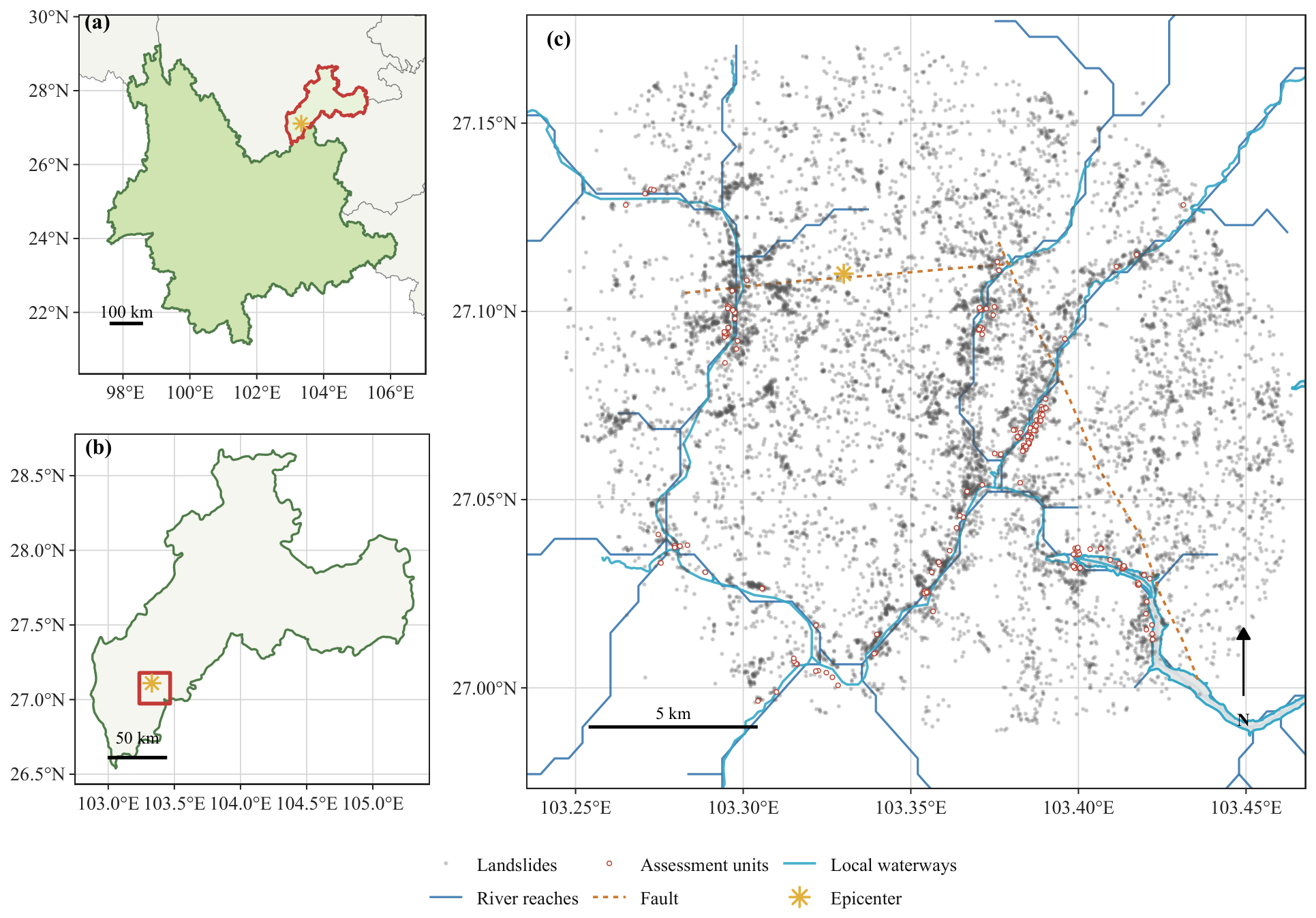
1. Introduction

Large landslides in high-relief gorge regions can become part of a disaster chain when failed material interacts with a river channel. Remote-sensing inventories document these slope failures, but they do not by themselves indicate which mapped objects should be examined first for river blockage or dammed-lake relevance. After mapping, the scientific question changes from locating landslides to prioritizing objects that warrant closer inspection for channel-coupled consequences [1,2,3,4,5].

This task begins after the inventory has been made. Inventory mapping asks where landslides occurred; susceptibility mapping estimates where failures may occur in the future. Post-inventory river-blockage prioritization asks a different question: among mapped failures, which objects have enough material, terrain, waterway, and river-network evidence to justify closer secondary-hazard review?

This distinction matters because reference evidence for disaster-chain relevance is geographically sparse and heterogeneous. Public reports, remote-sensing indicators, waterway mapping, and standardized river-network attributes record different signals at different spatial supports. A table note can record a missing value, but it cannot systematically distinguish absent evidence from evidence that a source did not observe or report. The knowledge graph (KG) addresses this gap by attaching provenance and post-scoring evidence status to relations, so that both prioritization decisions and missing evidence remain inspectable after ranking.

A conventional table can store the variables used for a final score, including area, estimated volume, slope, river distance, discharge, upstream area, and river order. The KG also records how a landslide becomes assessable by the typed eligibility relations, the source of each relation, and the public event context attached only after scoring. This route remains explicit while the final score can still be exported as a table.

We frame the problem as remote-sensing post-inventory disaster-chain prioritization. The framework occupies the step between inventory production and detailed secondary-hazard assessment. It does not replace susceptibility mapping, image interpretation, field investigation, dam-geometry reconstruction, or hydraulic modeling. Event-specific physics-based models for rainfall-triggered shallow-landslide initiation and movement, such as dynamic coupling of the Transient Rainfall Infiltration and Grid-Based Regional Slope-Stability (TRIGRS) and Rapid Mass Movement Simulation (RAMMS) models, are complementary analyses outside the present graph-based ranking [6]. Instead, it converts mapped landslides into assessment units whose material, terrain, waterway, river-network, and provenance context can be inspected together, allowing limited expert resources to be directed to a transparent shortlist. Its contribution is traceability: the graph preserves evidence chains and evidence gaps that a static score table or spreadsheet can only summarize after export.

Accordingly, this study has three objectives: (1) to define reproducible assessment units from a mapped inventory using explicit mechanism-oriented rules; (2) to provide a conservative relative-priority score and test its sensitivity to thresholds, correlated variables, normalization, and spatial concentration; (3) to retain queryable provenance and interpretation boundaries for every ranked unit. No score is interpreted as a probability of river blockage or as an independent confirmation of a landslide-dammed lake.

2. Related Work

Remote-sensing landslide inventories provide the object basis for post-event analysis. Machine-learning and deep-learning studies have improved the detection of landslides from remote-sensing images, and broader reviews show how central these methods have become in image interpretation [7,8,9]. In the Ludian case, the mapped inventory defines where slope failures occurred and makes object-level analysis possible [10]. River-blockage and dammed-lake assessment then requires evidence beyond the inventory polygon, including channel coupling, hydrologic position, rainfall and seismic context, and regional river-network structure. Open datasets such as the Advanced National Seismic System (ANSS) Comprehensive Earthquake Catalog (ComCat), Climate Hazards Group InfraRed Precipitation with Station data (CHIRPS), HydroRIVERS, and OpenStreetMap can provide this context, but they differ in spatial support, provenance, and uncertainty [11,12,13,14,15,16].

For the present problem, mapped landslide objects are already available. The harder step is to keep polygon geometry, material supply, channel coupling, hydrologic relevance, and contextual evidence connected after the inventory has been produced. Recent data-driven studies examine landslide susceptibility with optimized machine-learning models and with TRIGRS-based physical information introduced into machine learning [17,18]. These prediction-oriented approaches estimate susceptibility or event-process behavior, whereas post-inventory screening orders already mapped objects for a different follow-up task. Susceptibility models and inventory products therefore provide important inputs, and a graph-based representation extends them by retaining eligibility rules and evidence lineage for post-inventory river-blockage assessment [3].

The landslide-dam literature provides the physical basis for this prioritization. Classic and recent studies indicate that natural-dam formation and failure depend on coupled slope-channel processes. Relevant factors include material supply, valley geometry, river discharge, dam geometry, and failure mechanism [1,2,4,5]. Geographic information system (GIS)-based damming-susceptibility and dammed-lake studies further require joint consideration of landslide source areas, runout or deposition potential, and channel or lake-forming settings [19,20,21]. Regional studies of the Hongshiyan landslide dam provide context for landslide-river coupling, mitigation, and dam-development feasibility in the Niulanjiang setting [22,23,24,25].

These studies motivate the variables used here, but conventional GIS and index-based procedures generally combine layers into a susceptibility class, score, or map. They are effective for spatial screening, yet the final output does not necessarily retain the full chain from source polygon to threshold, waterway relation, river-reach linkage, score component, provenance, and later contextual evidence. This is not a numerical deficiency of GIS; it is an audit and data-lineage limitation when evidence sources have different spatial supports and when the assessment must be revisited after ranking.

KGs offer a way to represent entities, semantic classes, evidence sources, and typed relations as explicit analytical objects [26,27]. This matters for geospatial disaster-chain screening because inventory polygons, river reaches, rainfall grids, seismic records, local waterways, and literature-derived contextual evidence do not share the same provenance or validation status. Geographic KG studies emphasize formal representation of spatial entities, relations, states, and processes. Remote-sensing and disaster KG studies further show how heterogeneous geospatial evidence can be organized as queryable knowledge [28,29,30,31]. A typed graph model can preserve these distinctions while supporting evidence-path queries through standard graph representations and query languages [32,33].

The remaining gap is therefore representational and operational. Existing index or map outputs rarely keep eligibility rules, relation alignment, scoring evidence, provenance, post-scoring contextual evidence, and claim boundaries connected after ranking. A KG is appropriate for this task because the objects to be prioritized are mapped landslides linked to channels, river reaches, source datasets, and contextual flags, and because these links must remain queryable when an expert reviews an individual case. The KG is not claimed to improve the arithmetic of the score. We assess it as an audit structure by constructing units under typed mechanism rules, ordering them with a conservative score, checking contextual agreement without direct label leakage, and retrieving the evidence path behind each result.

3. Study Area and Data

The study focuses on the Ludian-Zhaotong-Niulanjiang alpine-gorge setting in northeastern Yunnan, Southwest China. The area lies in a plateau-to-gorge transition characterized by strong local relief, steep and deeply incised valleys, active seismic deformation, and slopes affected by fractured rock and surficial deposits. The Niulanjiang river system creates narrow channel settings in which earthquake-induced slope failures can interact with valley-floor infrastructure and river flow. The 2014 Ludian earthquake generated a dense landslide inventory, and the Hongshiyan landslide dam demonstrated the regional relevance of coupled slope-channel processes and emergency dam-risk management [22,23,24].

These characteristics make the area suitable for post-inventory screening, but they also create spatial dependence. Nearby polygons may represent related failures, share the same river reach, or repeatedly sample the same named regional context. Apparent agreement with public evidence can therefore be inflated if each polygon is treated as independent. The landslide inventory is derived from the Ludian dataset [10], and post-scoring disaster-chain context is drawn from Hongshiyan and Niulanjiang studies [22,24,25]. Cluster-level checks are used later to make this dependence explicit.

The data design separates construction inputs from contextual indicators attached only after scoring. Landslide, terrain, seismic, rainfall, local waterway, and standardized river-network data are used to build and score assessment units. Three regional terms derived from public Hongshiyan/Niulanjiang materials are then matched against the nearest-waterway name field to assign the external-context flag. We use “silver” for an internally defined multi-evidence consistency label, not externally verified ground truth. The name field is not used in the Mechanism-Balanced Evidence Index (MBEI), but it comes from the same OpenStreetMap (OSM) extract as the local-waterway screen; the flag is therefore not source-independent polygon-level evidence.

Table 1. Data sources, spatial support, analytical roles, and principal uncertainties. Post-scoring contextual evidence is excluded from screening and scoring.

Data Source	Spatial Support/Resolution	KG Layer	Use	Main Uncertainty
Ludian inventory (Zenodo)	Object polygons with polygon-derived attributes; source-image pixel size is not supplied with the archived polygons	Inventory and terrain context	Build and score	Mapping, boundary, and attribute uncertainty are inherited from the published inventory; object-level positional accuracy is not reported, and polygons are not river-blockage labels.
USGS ComCat	Event points and catalog attributes	Seismic context	Context construction	Location, magnitude, and completeness vary by event and catalog period.
CHIRPS daily rainfall	Daily 0.${05}^{\circ }$ grid	Rainfall context	Context construction	Gridded rainfall smooths orographic and local convective extremes.
OpenStreetMap Overpass extract	Vector waterways and water polygons extracted on 5 July 2026	Local waterway context	Build and screen	OSM provides no uniform positional-accuracy guarantee; small or unmapped channels may be missed.
HydroRIVERS river network	Reach centerlines derived from 15 arc-second hydrography	Standardized river-network context	Build and score	Generalized centerlines and modeled attributes do not resolve local channel width, banks, or hydraulic controls.
Hongshiyan/Niulanjiang contextual terms	Three regional name strings matched to the nearest OSM waterway name	Post-scoring contextual indicator	Diagnostic check only	The indicator is geographically concentrated, shares the OSM source with the waterway layer, and cannot provide positive or negative polygon-level attribution.

Abbreviations: KG, knowledge graph; USGS, U.S. Geological Survey; ComCat, Comprehensive Earthquake Catalog; CHIRPS, Climate Hazards Group InfraRed Precipitation with Station data; OSM, OpenStreetMap.

summarizes the data sources and their analytical roles.

Figure 1 shows the multi-scale location and mapped spatial evidence used in the study.

4. Methods

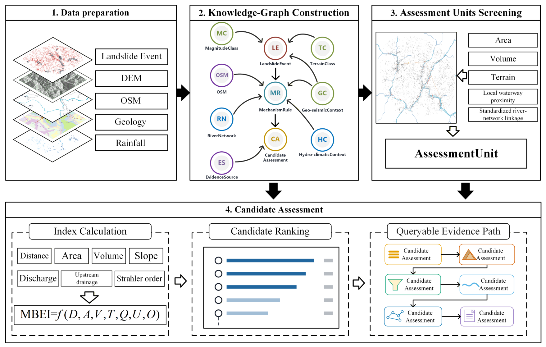
The method follows the sequence in Figure 2. Data preparation converts the landslide inventory and open environmental layers into spatial records, and KG construction represents those records as typed nodes, relations, and properties. In this paper, screening refers to filtering inventory objects into assessment units, whereas ranking or prioritization refers to ordering those retained units with MBEI. Audit and evaluation refer to post-ranking checks, evidence-path retrieval, contextual-evidence diagnostics, and interpretation-limit records. These terms separate construction of the assessment universe from the numerical shortlist and from later evidence inspection.

Figure 2. Overall analytical route. The method separates data preparation, KG construction, assessment-unit screening, evidence indexing, priority ranking, and evidence-path audit; the abbreviated KG nodes are defined in Table 2 and expanded in Figure 3. DEM denotes digital elevation model, OSM denotes OpenStreetMap, and MBEI denotes Mechanism-Balanced Evidence Index.

Figure 2. Overall analytical route. The method separates data preparation, KG construction, assessment-unit screening, evidence indexing, priority ranking, and evidence-path audit; the abbreviated KG nodes are defined in Table 2 and expanded in Figure 3. DEM denotes digital elevation model, OSM denotes OpenStreetMap, and MBEI denotes Mechanism-Balanced Evidence Index.

Table 2. KG construction and operation protocol. Numeric measurements remain properties, while reusable mechanism evidence and audit information are represented as typed graph objects or relations.

KG Element	Construction Rule	Analytical Use
LandslideEvent	Mapped polygon with area, volume, slope, date, and distance properties.	Core object for reference-set construction and ranking.
TerrainClass and MagnitudeClass	Thresholded slope, area, and volume link to shared classes.	Represent reusable mechanism evidence.
OSMWaterway and HydroRIVERSReach	Proximity and nearest-reach rules create channel links.	Encode channel-coupling and hydrologic support.
MechanismRule	Requires supply, terrain, waterway, and river-reach evidence.	Construct eligible assessment units.
CandidateAssessment	Assessment unit materialized after screening; stores score and rank after MBEI calculation.	Connects the retained unit to queryable evidence paths.
EvidenceSource and interpretation-limit notes	Contextual flags and interpretation limits are attached after scoring.	Support provenance, contextual-evidence checking, and audit.

Abbreviation: MBEI, Mechanism-Balanced Evidence Index.

Table 2. KG construction and operation protocol. Numeric measurements remain properties, while reusable mechanism evidence and audit information are represented as typed graph objects or relations.

KG Element	Construction Rule	Analytical Use
LandslideEvent	Mapped polygon with area, volume, slope, date, and distance properties.	Core object for reference-set construction and ranking.
TerrainClass and MagnitudeClass	Thresholded slope, area, and volume link to shared classes.	Represent reusable mechanism evidence.
OSMWaterway and HydroRIVERSReach	Proximity and nearest-reach rules create channel links.	Encode channel-coupling and hydrologic support.
MechanismRule	Requires supply, terrain, waterway, and river-reach evidence.	Construct eligible assessment units.
CandidateAssessment	Assessment unit materialized after screening; stores score and rank after MBEI calculation.	Connects the retained unit to queryable evidence paths.
EvidenceSource and interpretation-limit notes	Contextual flags and interpretation limits are attached after scoring.	Support provenance, contextual-evidence checking, and audit.

Abbreviation: MBEI, Mechanism-Balanced Evidence Index.

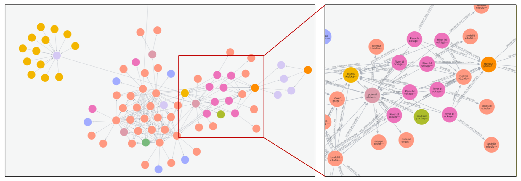
Figure 3. Illustrative Neo4j display subset of the constructed KG. The displayed subset shows representative relation types and evidence-path structure linking landslide events, mechanism rules, CandidateAssessment nodes, waterway and river-network context, and post-scoring evidence sources.

Figure 3. Illustrative Neo4j display subset of the constructed KG. The displayed subset shows representative relation types and evidence-path structure linking landslide events, mechanism rules, CandidateAssessment nodes, waterway and river-network context, and post-scoring evidence sources.

4.1. Data Preparation and Evidence Layers

The input layer starts with mapped landslide polygons rather than raw image detection. For each landslide, the KG record stores a stable identifier and derives or joins variables that describe material supply, terrain setting, local channel opportunity, standardized river-network context, and broader triggering background. Area (${\mathrm{m}}^2$), estimated volume (${\mathrm{m}}^3$), slope (degrees), river-network distance ($\mathrm{m}$), discharge (${\mathrm{m}}^3{\mathrm{s}}^{-1}$), upstream drainage area (${\mathrm{km}}^2$), and Strahler order (a dimensionless ordinal integer) are retained as numeric fields for scoring.

The environmental layers have distinct roles. OpenStreetMap provides locally mapped channels and water bodies and is used for the operational near-waterway screen. HydroRIVERS provides a standardized, topologically consistent reach association and supplies discharge, upstream drainage area, and river order for ranking and audit. The two products are complementary rather than interchangeable: OSM can retain local features that are absent from a generalized global network, whereas HydroRIVERS offers consistent hydrologic attributes but does not represent local channel geometry. Rainfall and seismic records provide regional hydroclimatic and seismic context. Lithologic information remains outside the final MBEI score, while geological or fault information is used as background context where available.

4.2. Knowledge-Graph Construction

KG construction transforms the prepared records into typed entities and relations. Each mapped polygon becomes a LandslideEvent node. Shared mechanism nodes represent magnitude, terrain setting, local waterway context, standardized river-network reach, hydroclimatic context, seismic context, and the rule schema used for later assessment. Continuous measurements remain node or relation properties so that the final score can still be exported and reproduced as a table.

Typed relations are created from deterministic spatial or attribute rules. A landslide is linked to magnitude and terrain classes by thresholded attributes, to local waterway context by proximity, and to a standardized river reach by nearest-reach association. Rainfall and seismic context are attached as background relations rather than score terms. The MechanismRule schema is used later to materialize assessment units as CandidateAssessment nodes.

The KG is used as an assessment structure rather than a graphical restatement of tabular variables. It records the typed relations available for later screening and ranking, and it keeps the source of each relation attached to the graph. A table can hold the seven exported score values; the KG additionally encodes the eligibility path from LandslideEvent to MechanismRule to CandidateAssessment. Table 2 lists the construction elements, and Figure 3 illustrates the Neo4j display subset used for evidence-path inspection.

4.3. Assessment-Unit Screening

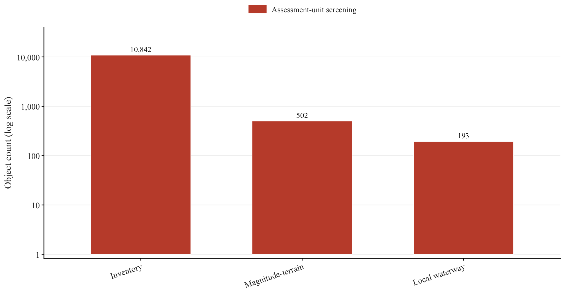
Assessment-unit screening creates CandidateAssessment nodes from KG relations already constructed. The screening rules are predefined operational screens rather than fitted physical failure thresholds. The area threshold of 13,446.6 m² is the 95th percentile of the complete 10,842-object inventory, and the volume threshold of 55,389.2 m³ is the corresponding 90th percentile. They retain the upper tail of mapped material supply. A minimum slope of ${20}^{\circ }$ excludes very gentle settings without implying a universal critical angle, and the 300 m OSM-waterway distance is a screening buffer for possible channel or water-body interaction rather than a runout or blockage-distance criterion. The standardized river-network linkage then adds hydrologic attributes and a river-reach relation to the retained units. When the pre-ranking evidence requirements are satisfied, the MechanismRule node connects to a CandidateAssessment node for that assessment unit.

These thresholds are applied to the original variables before the log transformation used for ranking. They are defined independently of the Hongshiyan/Niulanjiang reports. The strict setting uses the area 95th percentile, volume 95th percentile, slope $\ge {25}^{\circ }$, and waterway distance $\le 200$ m; the loose setting uses the area 90th percentile, volume 80th percentile, slope $\ge {20}^{\circ }$, and waterway distance $\le 500$ m. These alternatives test selection dependence and are not tuned definitions.

The 193 retained units form a reference screening set, not an exhaustive inventory of landslides capable of blocking rivers. Objects outside the set fail at least one open-data screening condition, but their exclusion does not establish the absence of channel interaction or damming potential. Smaller, more mobile, poorly mapped, or locally channel-connected landslides may still matter; those cases require expert interpretation, high-resolution imagery, field evidence, runout and dam geometry, river hydraulics, or hydrodynamic modeling.

The relation-constrained screening step can be summarized as an indicator over four mechanism requirements: material supply, terrain setting, local waterway proximity, and standardized river-reach linkage. Specifically, ${\mathrm{Supply}}_i=1$ when the original area and volume satisfy the reference thresholds, ${\mathrm{Terrain}}_i=1$ when slope is at least ${20}^{\circ }$, ${\mathrm{Waterway}}_i=1$ when the nearest OSM waterway or water polygon is within 300 m, and ${\mathrm{RiverReach}}_i=1$ when a nearest HydroRIVERS reach is available. The OSM relation is used for the near-waterway screen, whereas HydroRIVERS supplies the river-network distance and hydrologic attributes used for ranking.

$$R_i=I[{\mathrm{Supply}}_i\wedge {\mathrm{Terrain}}_i\wedge {\mathrm{Waterway}}_i\wedge {\mathrm{RiverReach}}_i]$$

(1)

Table 3. Screening protocol from inventory objects to the reference assessment set. Area and volume are inventory percentiles; slope and waterway distance are operational screens rather than universal physical thresholds. HydroRIVERS linkage enriches the 193 units after the count-reducing stages.

Stage	Rule	Physical Meaning	Count
Remote-sensing landslide inventory	All mapped landslide objects in the Ludian inventory	Starting inventory of mapped slope failures	10,842
Large-landslide screening rule	area ≥ 13,446.6 m2 (95th percentile); volume ≥ 55,389.2 m3 (90th percentile); slope ≥ ${20}^{\circ }$	Upper-tail material supply and minimum operational terrain screen	502
Near-waterway relation constraint	distance to nearest OSM waterway or water polygon ≤ 300 m	Operational opportunity screen for channel or water-body interaction	193

includes only the steps that change the number of retained landslides. After the near-waterway screen, the same 193 landslides are linked to standardized river-network context and represented as assessment units. The table therefore contains one 193-object reference set rather than a second 193-object filtering stage. In this dataset, every near-waterway object could be linked to a HydroRIVERS reach; RiverReach is required for scoring and audit enrichment in the reference graph and serves as an enrichment relation rather than a count-reducing filter.

4.4. MBEI Calculation and Ranking

The primary ranking score is the Mechanism-Balanced Evidence Index (MBEI), a conservative equal-weight score over seven standardized mechanism-relevant variables. Equal weights are used as a transparent, non-optimized default because the available contextual labels are incomplete and unsuitable for weight fitting. This choice does not assert that the seven variables are physically independent or equally important. The same MBEI score is used for ranking, ablation, relation-alignment controls, and sensitivity checks so that the reported method has a single numerical identity.

For assessment unit i, the Mechanism-Balanced Evidence Index is:

$$S_{\mathrm{MBEI},i}={\displaystyle \frac{z_{iD}+z_{iA}+z_{iV}+z_{iT}+z_{iQ}+z_{iU}+z_{iO}}{7}}$$

(2)

Here $d_i$ is the distance from assessment unit i to its associated HydroRIVERS reach, measured in meters. The term $z_{iD}$ is the inverted standardized distance, $z_{iA}$ is standardized landslide area, $z_{iV}$ is standardized estimated volume, $z_{iT}$ is standardized slope, $z_{iQ}$ is standardized discharge, $z_{iU}$ is standardized upstream drainage area, and $z_{iO}$ is standardized Strahler order. Area, volume, discharge, and upstream area are log-transformed before min–max normalization using their numerical values in the stated units; all minima and maxima are calculated over the set S being ranked.

All seven variables are normalized to the unit interval after the stated transformations; the distance term is inverted so that shorter river-network distance receives a larger score. Log transformation reduces the leverage of strongly right-skewed area and hydrologic variables, whereas min–max normalization preserves their ordering but remains sensitive to sample extremes. Retained assessment units are sorted by descending MBEI, and the score and rank are stored on the CandidateAssessment node. The result is a relative priority within the selected reference set, not a probability, susceptibility value, or event prediction.

For positive-direction variables $j\in \{A,V,T,Q,U,O\}$, define the transformed value exactly as implemented:

$${\overline{x}}_{ij}=\left\{\begin{array}{cc}\ln \left(1+\max \{x_{ij},0\}\right),\hfill & j\in \{A,V,Q,U\},\hfill \\ x_{ij},\hfill & j\in \{T,O\}.\hfill \end{array}\right.$$

(3)

The $\log (1+x)$ form is defined at zero and matches the nonnegative clipping used in the analysis code. The standardized component is then:

$$z_{ij}={\displaystyle \frac{{\overline{x}}_{ij}-{\min }_{r\in S}\left({\overline{x}}_{rj}\right)}{{\max }_{r\in S}\left({\overline{x}}_{rj}\right)-{\min }_{r\in S}\left({\overline{x}}_{rj}\right)}}$$

(4)

For river-network distance, the standardized distance component is inverted:

$$z_{iD}=1-{\displaystyle \frac{d_i-{\min }_{r\in S}\left(d_r\right)}{{\max }_{r\in S}\left(d_r\right)-{\min }_{r\in S}\left(d_r\right)}}$$

(5)

After all variables and assessment units are exported, a full-feature table can reproduce the numerical ranking. For the reference ranking and its weight, correlation, and normalization diagnostics, S is the 193-unit reference set. For the strict and loose screening checks, S is the corresponding retained set, so the reported values in Table 10 are within-set diagnostics rather than directly comparable score magnitudes. The KG preserves the retained relations that create, rank, contextualize, and qualify each assessment unit.

Two additional diagnostics address redundancy and normalization sensitivity. First, Spearman correlations are calculated among the seven normalized components. The group-balanced four-domain score is defined as

$$S_{4,i}={\displaystyle \frac{1}{4}}\left[z_{iD}+{\displaystyle \frac{z_{iA}+z_{iV}}{2}}+z_{iT}+{\displaystyle \frac{z_{iQ}+z_{iU}+z_{iO}}{3}}\right].$$

(6)

It gives equal weight to river distance, combined material supply, slope, and combined hydrologic background, so strongly correlated variables do not automatically receive repeated domain weight. Second, a robust MBEI clips all seven components before min–max normalization. Let $v_{iD}=d_i$ and $v_{ij}={\overline{x}}_{ij}$ for $j\in \{A,V,T,Q,U,O\}$; with $q_{p,j}$ denoting the pth quantile over S, the clipped value is

$$v_{ij}^{\left(c\right)}=\min \left\{\max \left(v_{ij},q_{0.01,j}\right),q_{0.99,j}\right\}.$$

(7)

The clipped distance is then min–max normalized and inverted, while the other six clipped variables are normalized in the positive direction. Both alternatives use the same set-specific transformation boundaries and are compared with the reference MBEI using Spearman rank correlation and Top-20 overlap; they are diagnostics rather than replacement models selected against contextual labels.

4.5. Post-Ranking Evidence-Path Audit and Evaluation

Evaluation begins only after assessment units have been screened and ranked. The post-ranking checks examine contextual agreement, dependence on mechanism relations, robustness to spatial and weighting choices, and recoverability of evidence paths.

The external-context label is assigned after ranking from the nearest-waterway name field. A regular-expression match checks for any of three curated Chinese name strings corresponding to Hongshiyan, Niulanjiang, or dammed lake; a match sets $E_i=1$, while a missing or unmatched name sets $E_i=0$. The waterway name is excluded from screening and MBEI scoring. In the reference set, 83 of the 193 units carry this named regional-context flag. The remaining 110 units are unlabeled because no match was found; they are not negative cases. Because the flag uses an OSM name attribute, it is a post-scoring contextual indicator rather than source-independent event evidence.

Because these contextual terms are concentrated around known river settings, cluster-level evaluation is used as a conservative check against inflation from repeated nearby assessment units.

The multi-evidence consistency label uses nine binary dimensions: HydroRIVERS distance within 300 m and within 100 m; area, volume, slope, discharge, and upstream drainage area at or above their respective upper quartiles in S; Strahler order at least 6; and the named regional-context flag $E_i$. If these indicators are $b_{im}$, then

$$M_i=I\left({\displaystyle \sum _{m=1}^9}{b}_{im}\ge 6\right).$$

(8)

Composite relevance for normalized discounted cumulative gain (NDCG) is defined as twice the external-context indicator plus this multi-evidence indicator. It is a contextual-evidence ordering diagnostic, not an independent event-confirmation metric. External precision at rank K (P@K) reports the fraction of the top-K units with $E_i=1$, whereas Silver P@K reports the fraction with $M_i=1$. Because $M_i$ includes normalized mechanism variables and $E_i$ among its nine dimensions, Silver P@K is a consistency diagnostic rather than independent validation.

The contextual composite relevance used by NDCG is:

$$re{l}_i=2E_i+M_i$$

(9)

Discounted cumulative gain at rank K (DCG@K) and ideal discounted cumulative gain at rank K (IDCG@K) are used to calculate NDCG@K:

$$DCG@K={\displaystyle \sum _{i=1}^K}{\displaystyle \frac{2^{re{l}_i}-1}{{\log }_2(i+1)}},NDCG@K=DCG@K/IDCG@K$$

(10)

where $IDCG@K$ is obtained by sorting the relevance values of all units $i\in S$ in descending order and taking the first K positions.

$$ExternalP@K={\displaystyle \frac{1}{K}}{\displaystyle \sum _{i=1}^K}I(E_i=1),SilverP@K={\displaystyle \frac{1}{K}}{\displaystyle \sum _{i=1}^K}I(M_i=1).$$

(11)

For evidence-layer tests, the seven MBEI components are grouped into three layers. The river-entry layer contains the inverted standardized river-network distance $z_{iD}$. The supply-mobility layer combines the standardized area, volume, and slope components ($z_{iA}$, $z_{iV}$, and $z_{iT}$). The hydrologic-background layer combines the standardized discharge, upstream drainage area, and Strahler-order components ($z_{iQ}$, $z_{iU}$, and $z_{iO}$). The equal-layer, removed-layer, and single-layer tests examine whether these groups are necessary or sufficient under contextual-evidence evaluation; they serve as diagnostic variants rather than additional proposed scoring methods.

The reduced-feature comparators use the same set S and normalized components. The area–river-distance score is $0.5z_{iA}+0.5z_{iD}$; the hydrologic-context score is $0.30z_{iD}+0.25z_{iQ}+0.25z_{iU}+0.20z_{iO}$; the river-network-distance comparator is $z_{iD}$; and the local-waterway-distance comparator is the inverted min–max normalized distance to the nearest OSM waterway or water polygon. These definitions keep the comparison transparent and separate the HydroRIVERS and OSM distance roles.

For the alternative-weight sensitivity experiment, a sampled weight vector produces

$$S_i^{\left(w\right)}=\sum _{j\in \{D,A,V,T,Q,U,O\}}{w}_j{z}_{ij}.$$

(12)

Equal weights are locally perturbed and renormalized rather than refitted to contextual-evidence labels:

$$w_j^{\left(0\right)}=1/7,{\tilde{w}}_j={\displaystyle \frac{w_j^{\left(0\right)}(1+{ϵ}_j)}{{\sum }_{k=1}^7{w}_k^{\left(0\right)}(1+{ϵ}_k)}},{ϵ}_j\sim U(-0.2,0.2).$$

(13)

For the broad positive-weight experiment, the normalized vector is drawn as $w^{\left(b\right)}\sim \mathrm{Dirichlet}\left(25w^{\left(0\right)}\right)$. All seven weights are positive and sum to one; the concentration parameter preserves the equal-weight vector as the center of the draw distribution.

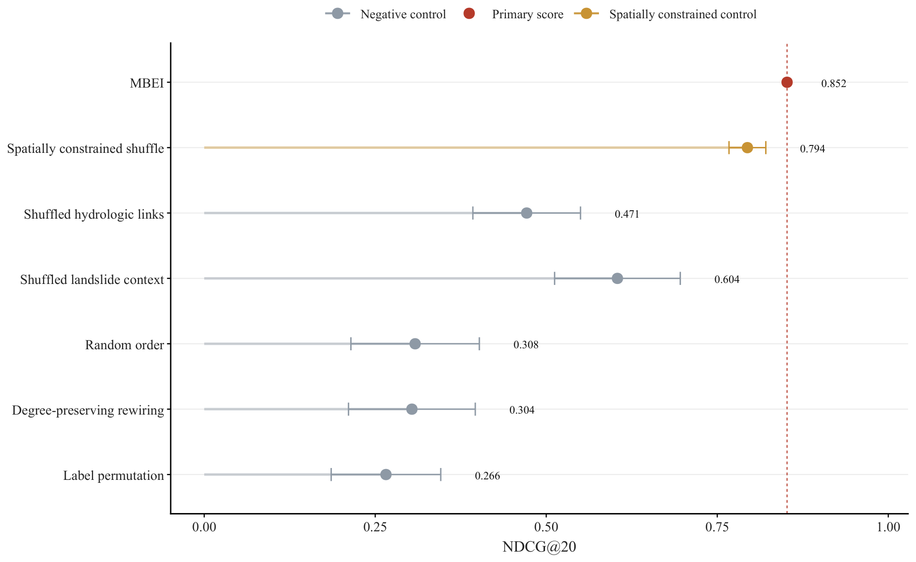
Relation-alignment controls include random ordering, shuffled hydrologic links, shuffled landslide-context links, degree-preserving rewiring, spatially constrained shuffling, and label permutation. Random ordering and label permutation test the reference set and contextual labels alone. Shuffled links and degree-preserving rewiring test whether relation alignment matters beyond graph density. The spatially constrained shuffle keeps nearby geographic context while disrupting object-level relation alignment. It is treated as a strong geographic-control case rather than a trivial failure case.

The screening-rule sensitivity uses three predefined sets of assessment units. The reference setting follows Table 3. The strict setting tightens the waterway distance to 200 m and uses a stricter volume and slope screen. The loose setting relaxes the magnitude and waterway-distance screens to include a broader set of objects. These settings test threshold dependence and are predefined before external-context labels are evaluated.

Cluster-level evaluation groups assessment units by standardized river reach and a 250 m Universal Transverse Mercator (UTM) grid cell before evaluation. The evidence-source exclusion check keeps Hongshiyan/Niulanjiang contextual evidence out of assessment-unit construction and scoring, then uses it only for post-scoring consistency checks. Traceability is also evaluated after ranking. For each ranked assessment unit, the graph retrieves the entry rule, score components, source datasets, local waterway relation, standardized river-reach relation, post-scoring contextual-evidence status, and interpretation-limit notes. Native KG traceability is the fraction of ranked units for which this chain is stored as linked graph relations. For a Top-K set, if $c_i$ is the number of the eight audit-path elements retrievable for unit i, reconstructed audit elements are $K^{-1}{\sum }_i{c}_i$, reconstructed coverage is ${\left(8K\right)}^{-1}{\sum }_i{c}_i$, and complete reconstruction is $K^{-1}{\sum }_{i}I(c_i=8)$. Evidence dims is the mean count of nine predefined evidence dimensions: HydroRIVERS support within 300 m and 100 m, upper-quartile area, upper-quartile volume, upper-quartile slope, upper-quartile discharge, upper-quartile upstream area, high Strahler order, and named hazard or waterway context.

Ranking, ablation, and negative controls evaluate the ordered shortlist against contextual labels. Robustness, exclusion-check, evidence-path, and case analyses test whether the ranking remains inspectable as a KG-based assessment representation.

5. Results

Across the tests, the ranking is driven largely by spatial-hydrologic context, while the KG keeps that ranking traceable. The subsections below move from the retained assessment units to ranking behavior, relation dependence, robustness, and evidence-path audit.

5.1. Screened Assessment Units and Primary Ranking

The reference set was fixed before ranking. Relation-constrained screening retained mapped landslides with material-supply potential, a basic topographic setting, local waterway proximity, and standardized river-network linkage. Hongshiyan/Niulanjiang contextual evidence was used only after ranking, so public-report matches did not enter the screening rules or MBEI calculation. Table 3 summarizes the screening protocol, and Figure 4 illustrates the corresponding reduction in object count.

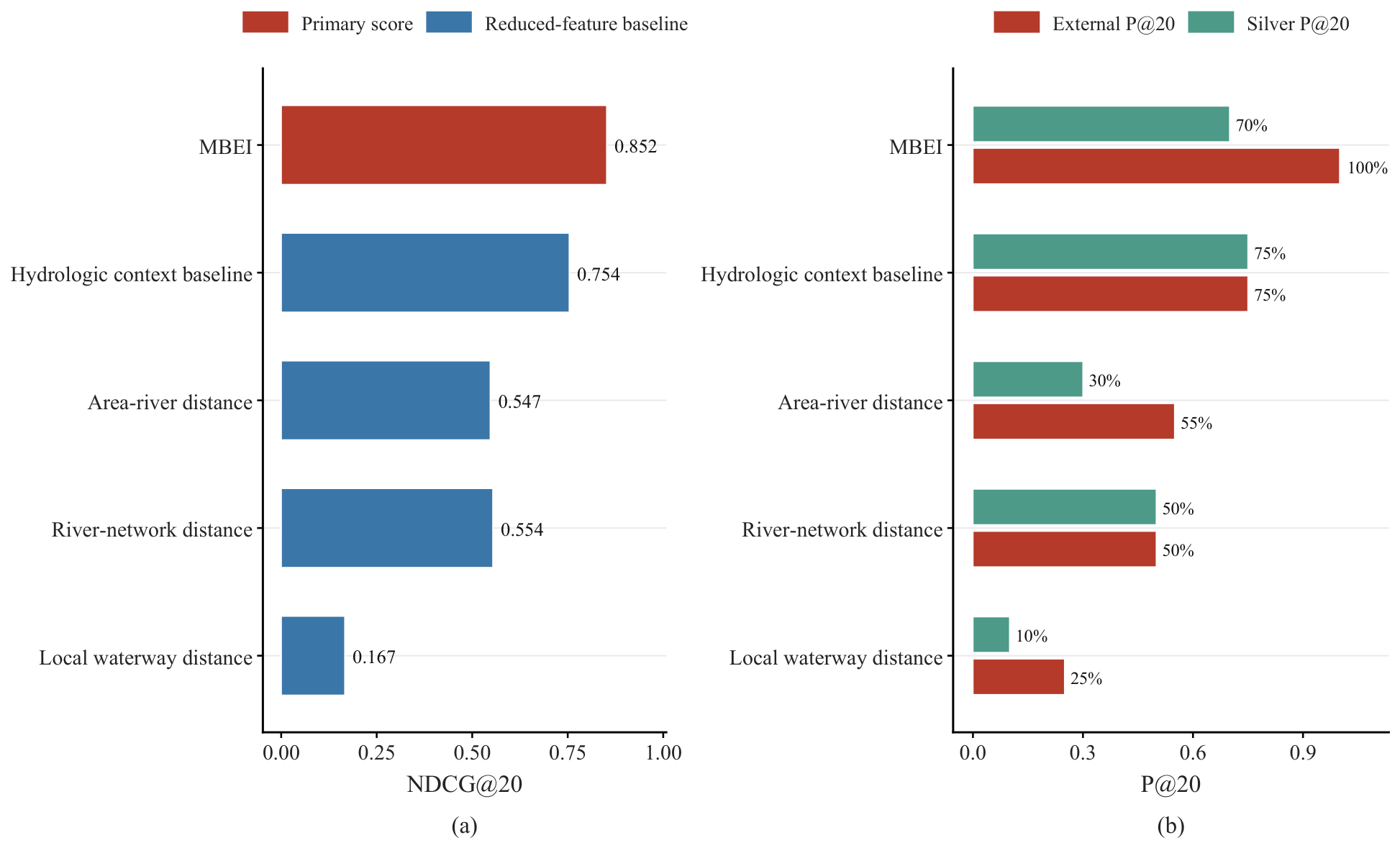
In the reference setting, MBEI placed many units carrying contextual-evidence flags near the top of the shortlist. Its NDCG@20 and External P@20 were higher than those of the tested reduced-feature comparators, while its Silver P@20 was slightly lower than the hydrologic comparator. These values describe agreement with incomplete regional-context and internal-consistency labels, not predictive accuracy.

Table 4. Main Top-20 contextual-agreement comparison. Higher NDCG@20 indicates earlier placement of units carrying the composite contextual flag; External P@20 is the fraction with a named regional-context match, and Silver P@20 is an internal mechanism-consistency diagnostic. None is polygon-level predictive accuracy.

Method	NDCG@20	External P@20	Silver P@20
MBEI	0.852	100.0%	70.0%
Hydrologic context baseline	0.754	75.0%	75.0%
Area-river distance	0.547	55.0%	30.0%
River-network distance	0.554	50.0%	50.0%
Local waterway distance	0.167	25.0%	10.0%

Abbreviations: NDCG@20, normalized discounted cumulative gain at rank 20; P@20, precision at rank 20.

summarizes the comparison, with the same diagnostic values shown in Figure 5.

MBEI is retained as the primary ranking output because it avoids assigning additional prior weight to one mechanism group under contextual-evidence evaluation. All main-text ranking, ablation, relation-alignment, and sensitivity results use the same primary score.

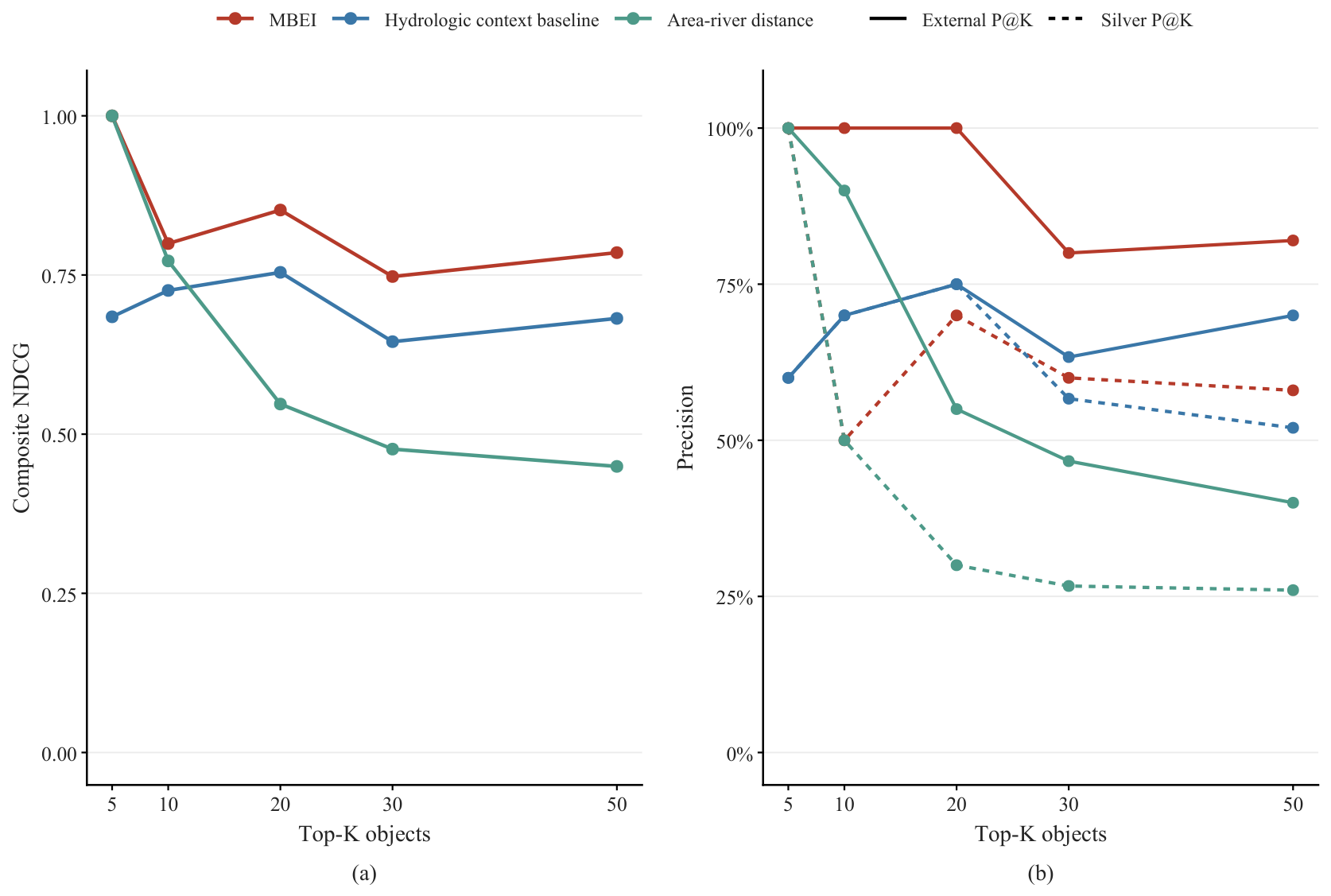
Across cutoffs, the output behaves as an ordered shortlist rather than a binary classifier. MBEI retained a high External P@K at the smaller cutoffs, followed by a lower value when the shortlist broadened to 50 units. Silver P@K was non-monotonic across the same cutoffs, so it is interpreted as an internal consistency diagnostic rather than a simple dilution curve.

Table 5. Cutoff stability for MBEI and reduced-feature baselines. Increasing K broadens the inspection list; NDCG@K describes contextual ordering, External P@K describes named regional-context matches, and Silver P@K describes internal mechanism consistency as defined in Section 4.5.

Method	K	NDCG@K	External P@K	Silver P@K
MBEI	10	0.799	100.0%	50.0%
MBEI	20	0.852	100.0%	70.0%
MBEI	50	0.785	82.0%	58.0%
Area-river distance	10	0.772	90.0%	50.0%
Area-river distance	20	0.547	55.0%	30.0%
Area-river distance	50	0.449	40.0%	26.0%
Hydrologic context baseline	10	0.726	70.0%	70.0%
Hydrologic context baseline	20	0.754	75.0%	75.0%
Hydrologic context baseline	50	0.682	70.0%	52.0%

summarizes this cutoff-dependent pattern, with the same values shown in Figure 6.

5.2. Mechanism Evidence and Relation Dependence

Material supply, terrain setting, local waterway proximity, and standardized river-network support contributed unevenly to the Top-20 ordering. The evidence-layer tests compare their combinations, the ablation tests remove or isolate graph layers, and the negative controls disrupt relation alignment while preserving parts of the object set or spatial context.

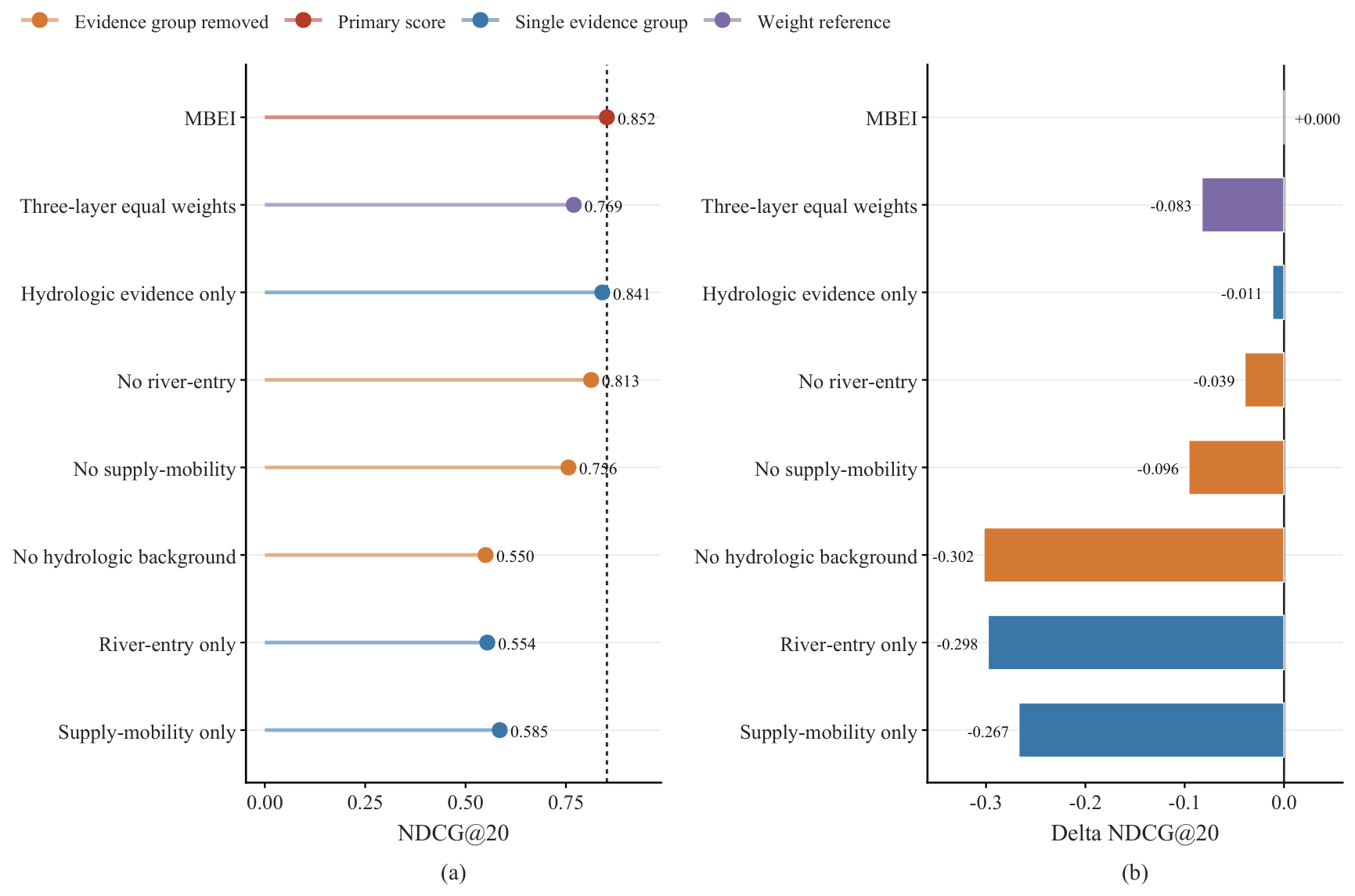
Hydrologic evidence accounted for most of the diagnostic signal in the mechanism-layer tests. The hydrologic-evidence-only test retained high contextual agreement, indicating that channel setting is a major source of the observed ordering in this case study. The other layers remained relevant for assessment traceability because they record whether material supply, terrain, and waterway relations support or weaken the hydrologic signal for a ranked unit.

Table 6. Contextual-agreement diagnostics for mechanism-evidence groups. Delta is relative to MBEI; negative values indicate lower NDCG@20 after changing or isolating a group. Silver P@20 remains an internal consistency measure as defined in Section 4.5.

Evidence Setting	Type	NDCG@20	Delta	External P@20	Silver P@20
MBEI	Primary score	0.852	+0.000	100.0%	70.0%
Three-layer equal weights	Alternative weighting	0.769	−0.083	85.0%	60.0%
No river-entry layer	Removed evidence group	0.813	−0.039	100.0%	60.0%
No supply-mobility layer	Removed evidence group	0.756	−0.096	75.0%	75.0%
No hydrologic-background layer	Removed evidence group	0.550	−0.302	55.0%	30.0%
River-entry only	Single evidence group	0.554	−0.298	50.0%	50.0%
Supply-mobility only	Single evidence group	0.585	−0.267	60.0%	35.0%
Hydrologic evidence only	Single evidence group	0.841	−0.011	100.0%	65.0%

summarizes the evidence-group tests, with Top-20 differences shown in Figure 7.

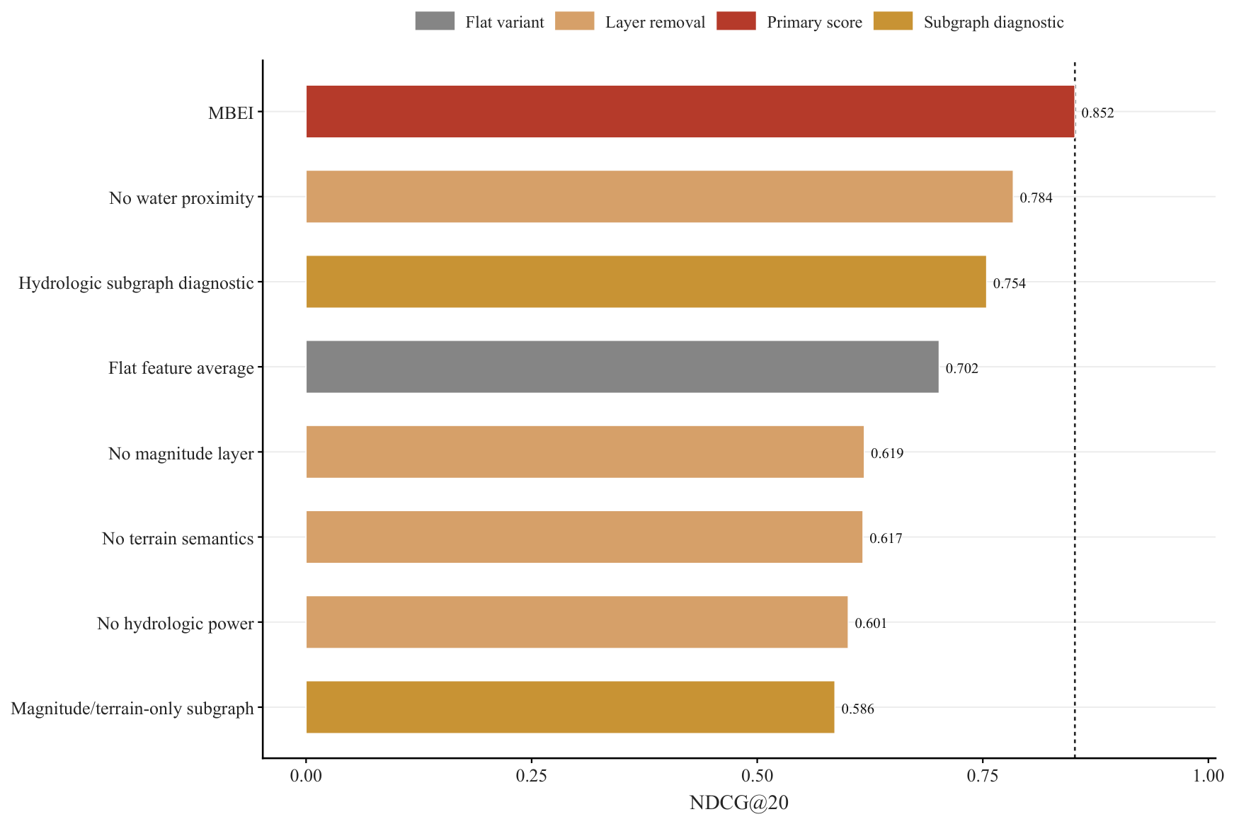
The layer-removal tests point in the same direction. Removing hydrologic background produced the largest decrease among the tested removals, while magnitude, terrain, and local waterway layers had smaller individual effects. This pattern reinforces the physical role of river-network position and discharge-related context. The KG preserves the material-supply, terrain, waterway, river-network, provenance, and interpretation-limit paths behind this signal for each assessment unit.

Table 7. Effect of removing evidence layers or restricting the available graph substructure. Lower NDCG@20 indicates weaker agreement with the composite contextual label after a layer is removed; Silver P@20 is the internal diagnostic defined in Section 4.5.

Variant	NDCG@20	Delta	External P@20	Silver P@20
MBEI	0.852	+0.000	100.0%	70.0%
Hydrologic subgraph only	0.754	−0.098	75.0%	75.0%
Magnitude/terrain-only subgraph	0.586	−0.266	60.0%	35.0%
No magnitude layer	0.619	−0.233	55.0%	55.0%
No terrain semantics	0.617	−0.235	70.0%	35.0%
No hydrologic power	0.601	−0.251	65.0%	35.0%
No water proximity	0.784	−0.068	90.0%	60.0%
Flat feature average	0.702	−0.150	75.0%	50.0%

summarizes the layer-removal and subgraph variants, while Figure 8 shows their NDCG@20 differences.

The negative controls separate relation alignment from background geography. Random order, label permutation, degree-preserving rewiring, and shuffled relations reduced contextual agreement. The spatially constrained shuffle stayed relatively high, showing that nearby geographic and hydrologic context already explains much of the observed label alignment. Typed graph relations therefore organize a strong spatial-hydrologic background while keeping the evidence inspectable.

Table 8. Sensitivity to relation alignment. Repeated controls are reported as mean ± standard deviation, and MBEI is a fixed reference. High values indicate stronger contextual agreement; the relatively high spatially constrained result shows how much local geography is retained. Silver P@20 follows Section 4.5.

Control	Runs	NDCG@20	External P@20	Silver P@20
MBEI	1	0.852	100.0%	70.0%
Random order	100	0.308 ± 0.094	43.5% ± 11.0%	21.9% ± 8.6%
Shuffled hydrologic links	100	0.471 ± 0.079	47.9% ± 9.2%	29.2% ± 7.1%
Shuffled landslide context	100	0.604 ± 0.092	76.3% ± 8.2%	48.6% ± 10.1%
Degree-preserving rewiring	100	0.304 ± 0.093	41.7% ± 10.5%	21.6% ± 8.2%
Spatially constrained shuffle	100	0.794 ± 0.027	95.1% ± 3.7%	59.8% ± 4.7%
Label permutation	100	0.266 ± 0.080	42.9% ± 11.8%	21.4% ± 7.7%

summarizes the relation-alignment controls, with NDCG@20 distributions shown in Figure 9.

5.3. Robustness to Weight, Screening Rules, and Spatial Effects

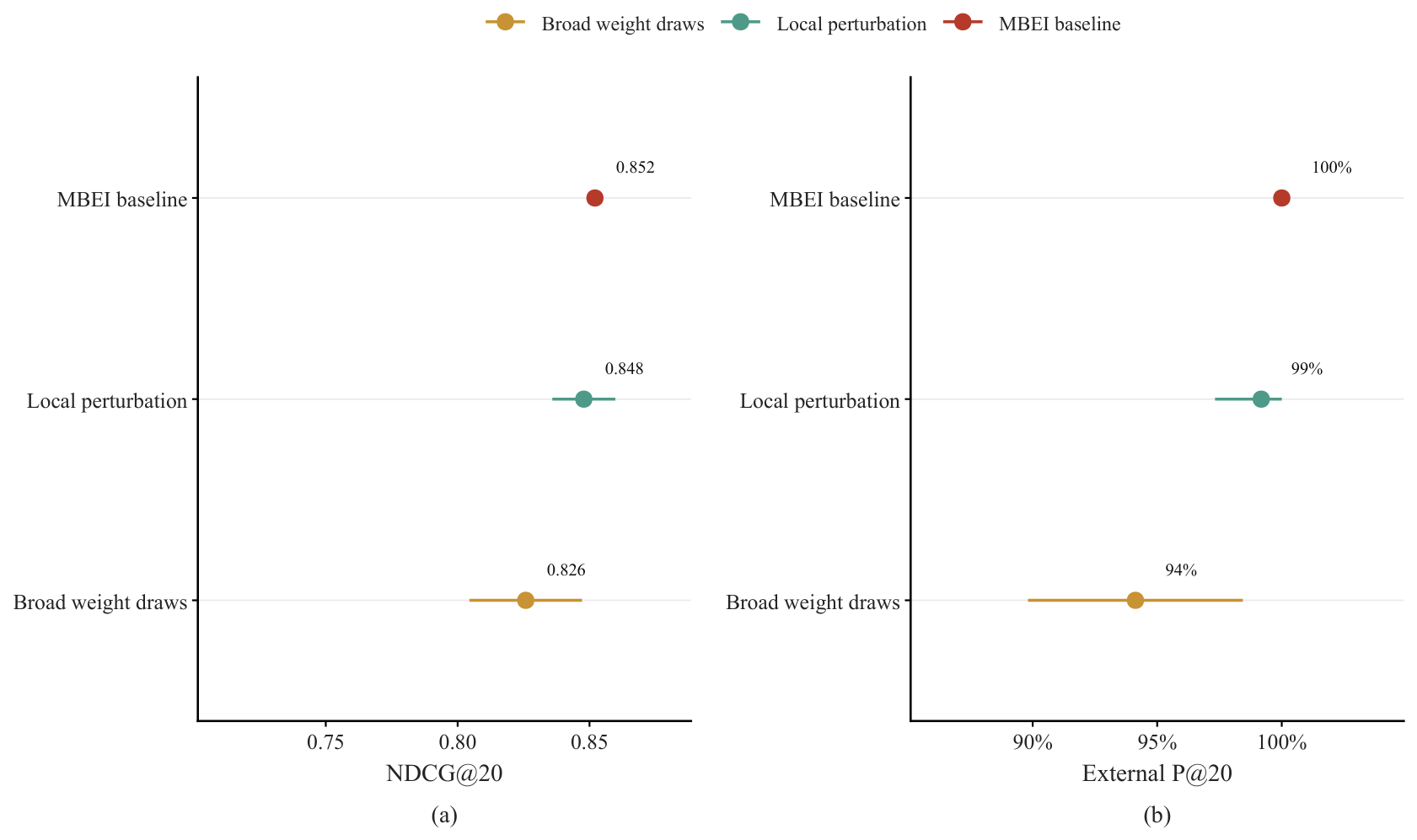
The robustness tests targeted three possible sources of overstatement: weight sensitivity, dependence on one screening-rule setting, and inflation from spatial clustering or contextual-evidence leakage. Weight perturbation asked whether random local changes and broad positive weight draws kept the contextual-ordering diagnostic close to the MBEI value. The local draws follow the bounded perturbation equation above, and the broad draws follow the stated Dirichlet distribution.

Weight perturbation produced only small changes around the MBEI baseline. The Top-20 ordering was stable under local and broad positive weight variations. Because the weights were defined independently of contextual labels, this analysis is a stability check rather than an optimization exercise.

Table 9. Alternative-weight sensitivity on the 193-unit reference set. The mean and standard deviation summarize repeated draws; values near the MBEI reference indicate that contextual ordering is not determined by one exact equal-weight vector.

Scenario	Runs	NDCG@20	External P@20
MBEI	1	0.852	100.0%
Random ± 20% local perturbation	200	0.848 ± 0.012	99.2% ± 1.9%
Broad positive weight draws	200	0.826 ± 0.021	94.1% ± 4.3%

and Figure 10 summarize the resulting spread around the MBEI reference.

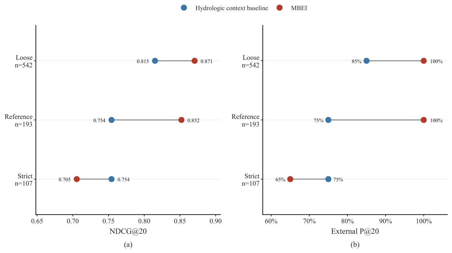
Screening-rule sensitivity showed that the diagnostic ordering changes when the retained unit set changes. The hydrologic comparator had the higher NDCG@20 under the strict setting, whereas MBEI had the higher value under the reference and loose settings. This transition indicates that apparent method differences depend on how much spatial-hydrologic context is already captured by the retained units. The reference set is used as a predefined assessment universe, and the strict and loose sets test how the interpretation responds to screening choices.

Table 10. Screening-rule sensitivity. The strict (107 units), reference (193), and loose (542) sets change the assessment universe rather than re-optimize the score. Higher values indicate stronger contextual agreement within each set; Silver P@20 follows Section 4.5.

Set	Count	Method	NDCG@20	External P@20	Silver P@20
Strict	107	MBEI	0.705	65.0%	55.0%
Strict	107	Hydrologic context baseline	0.754	75.0%	75.0%
Reference	193	MBEI	0.852	100.0%	70.0%
Reference	193	Hydrologic context baseline	0.754	75.0%	75.0%
Loose	542	MBEI	0.871	100.0%	75.0%
Loose	542	Hydrologic context baseline	0.815	85.0%	75.0%

compares the three settings, and Figure 11 visualizes the same sensitivity test.

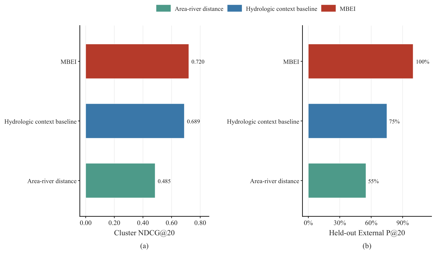
Cluster-level evaluation made the ranking more conservative. Nearby objects were grouped by standardized river reach and a 250 m UTM grid, reducing the effect of dense local inventories. After clustering, MBEI and the hydrologic comparator converged, consistent with nearby landslides sharing the same river setting and contextual evidence.

Table 11. Cluster-level and external-context exclusion checks. Clustering reduces repeated representation of nearby objects on the same river setting; the exclusion-check rows document procedural exclusion of named context from screening and scoring rather than independent validation. Silver P@20 follows Section 4.5.

Check	Method	NDCG@20	External P@20	Silver P@20
Cluster-level evaluation	MBEI	0.720	75.0%	60.0%
Cluster-level evaluation	Area-river distance	0.485	50.0%	35.0%
Cluster-level evaluation	Hydrologic context baseline	0.689	70.0%	65.0%
External-context exclusion check	MBEI	0.852	100.0%	70.0%
External-context exclusion check	Area-river distance	0.547	55.0%	30.0%
External-context exclusion check	Hydrologic context baseline	0.754	75.0%	75.0%

reports the cluster-level and external-context exclusion checks, and Figure 12 separates the two robustness views.

The external-context exclusion check documents procedural exclusion of Hongshiyan/Niulanjiang contextual evidence from screening and scoring. It is not an independent spatial evaluation. Residual geographic dependence remains possible because nearby assessment units may share the same river setting, but the check addresses the most direct leakage pathway.

5.4. Evidence-Path Audit and Representative Assessment Cases

The evidence-path analysis asks whether ranked assessment units retain their mechanism chain after scoring. For the Top-20 units, the KG stores the assessment rule, relation path, data source, external-evidence exclusion status, and interpretation-limit notes as linked audit information.

For example, a top-ranked CandidateAssessment node can retrieve the LandslideEvent identifier, the satisfied MechanismRule, the local waterway relation, the standardized river-reach link, the MBEI component values, the source datasets, and whether any contextual flag was attached after scoring.

Evidence-path completeness was near-complete for the Top-20 objects ranked by MBEI, and native traceability was retained through the graph schema. For each Top-20 assessment unit, the graph preserves the entry rule, supporting mechanism evidence, post-scoring contextual status, and the stated boundary of interpretation.

All retained assessment units can be audited through the KG after ranking.

Table 12. Native graph traceability and post hoc reconstruction of eight audit-path elements for the Top-20 units. Mean element count, coverage, and complete-path rate use the definitions in Section 4.5. The eight elements describe linked provenance and assessment relations; they are not the seven numeric MBEI score variables.

Method	Native Traceability	Reconst. Audit Elements	Reconst. Coverage	Complete Reconst.	Evidence Dims
MBEI	100.0%	7.95	99.4%	95.0%	6.30
Area-river distance	0.0%	7.70	96.2%	70.0%	4.85
Hydrologic context baseline	0.0%	7.95	99.4%	95.0%	5.75
Full-feature table	0.0%	8.00	100.0%	100.0%	6.10

compares whether the ranking output itself carries linked evidence paths or whether audit elements must be reconstructed after export. The eight audit-path elements are area class, volume class, slope class, OSM-waterway relation, HydroRIVERS-reach relation, CandidateAssessment relation, HydroRIVERS-support relation, and post-scoring external-context status. They are distinct from the seven numeric MBEI variables. For reduced-feature and full-feature table rankings, the audit-element counts are reconstructed from exported records rather than stored as native graph paths. Thus, the 75.0% path completeness reported for the example in Table 14 corresponds to six of eight retrievable elements.

The full-feature table row marks the boundary of the numerical claim. It can reproduce complete score components after export, while the KG stores assessment eligibility, post-scoring evidence status, provenance, and interpretation limits as queryable graph paths.

The representative cases show what the audit adds beyond a score. They are interpreted as assessment examples rather than verified river-blockage sources. Each case can be traced through material-supply indicators, terrain setting, local waterway context, standardized river-network support, CandidateAssessment records, post-scoring contextual flags, and interpretation-limit flags.

Table 13. Representative evidence-path cases. Scores and paths summarize evidence used for prioritized assessment under incomplete contextual-evidence conditions.

Case Type	Object ID	Score	Key Evidence	Evidence Path	Boundary
Complete high-priority path	05_201607:00459	0.931	A = 547196 m2; V = $11.31\times {10}^6 {\mathrm{m}}^3$; slope = ${66.5}^{\circ }$.	8 audit elements; 100.0%.	High-priority assessment unit
Date-context flag	02_201408:00230	0.900	A = 365958 m2; V = $6.95\times {10}^6 {\mathrm{m}}^3$; slope = ${56.9}^{\circ }$.	8 audit elements; 100.0%.	Date-context flag
Boundary-type case	07_201808:00142	0.832	A = 596126 m2; V = $12.54\times {10}^6 {\mathrm{m}}^3$; slope = ${33.3}^{\circ }$.	8 audit elements; 100.0%.	Complete path with weaker component evidence

lists high-priority assessment units, spatial duplicates, externally flagged low-ranked units, and incomplete evidence paths that require expert inspection.

Failure patterns are treated as assessment flags. Missing external support may reflect incomplete public reporting, while externally supported low-ranked units may reflect contextual evidence broader than the mapped polygon.

Table 14. Uncertainty and assessment-priority patterns. These examples are assessment flags, not verified errors.

Pattern	Example	Observation	Assessment Implication
High-ranked without external support	08_201908:00069	Score 0.659; no external-context label.	Assess public-record incompleteness.
Low-ranked with external support	01_201404:00044	Score 0.285; external support exists.	Boundary of deterministic scoring.
Spatial duplicate	02_201408:00377	Cluster 40850986_1360_11981 contains 12 objects.	Motivates cluster-level evaluation.
Incomplete evidence path	03_201410:00202	Path completeness 75.0%.	Flagged for expert assessment.

identifies units and river settings where expert interpretation is most valuable.

5.5. Correlation and Normalization Diagnostics

The component analysis confirms that equal weighting does not imply statistical independence. Area and estimated volume are perfectly rank-correlated in the retained set ($\rho =1.000$), as are HydroRIVERS discharge and upstream drainage area ($\rho =1.000$). Discharge and river order, and upstream area and river order, are also strongly correlated ($\rho =0.856$). These relationships mean that the reference MBEI gives repeated numerical representation to material-supply and hydrologic-background information.

The correlation-aware diagnostic nevertheless preserves most of the practical shortlist. Giving equal weight to four domains—river distance, combined material supply, slope, and combined hydrologic background—produces a Spearman rank correlation of 0.966 with the reference MBEI and retains 16 of the same Top-20 units (80%). The percentile-clipped normalization produces a rank correlation of 0.999 and retains all 20 reference units.

Table 15. Correlation, grouped-weight, and robust-normalization diagnostics for the 193 assessment units. Correlations describe redundancy among MBEI components; rank correlation and Top-20 overlap compare alternative diagnostic scores with the reference MBEI.

Diagnostic	Result	Top-20 Overlap	Interpretation
Area versus estimated volume	Spearman $\rho =1.000$	Not applicable	Material-supply variables are rank-redundant in this set.
Discharge versus upstream area	Spearman $\rho =1.000$	Not applicable	Two hydrologic attributes carry the same rank ordering.
Discharge/upstream area versus river order	Spearman $\rho =0.856$	Not applicable	Hydrologic-background variables are strongly related.
Four-domain group-balanced score	Rank $\rho =0.966$	16/20 (80%)	Most priorities persist after reducing repeated variable weight.
1st–99th percentile-clipped MBEI	Rank $\rho =0.999$	20/20 (100%)	The Top-20 is insensitive to the tested extreme-value treatment.

summarizes these results. They support the stability of the shortlist to extreme-value treatment, while the four-unit change under domain balancing shows that correlated variables should remain an explicit interpretation limit.

6. Discussion

6.1. Interpretation of the Ranking and KG Contribution

The ranking results show a strong hydrologic signal. The Hydrologic context baseline, hydrologic-evidence-only test, and spatially constrained shuffle indicate that river distance, upstream area, discharge-related context, and local spatial clustering are first-order controls on agreement with the available contextual labels. MBEI is designed to work with that physical setting rather than overwrite it. Its role is to organize the hydrologic signal together with non-hydrologic evidence, so that slope, material supply, terrain, waterway, provenance, and missing-evidence status can be inspected for each prioritized assessment unit.

The KG contribution is therefore not a claim of higher predictive performance. Once all variables are exported, a complete table can reproduce the numerical ranking. The graph instead supports native audit operations: it retrieves why an assessment unit was created, which score components were used, which source datasets supplied the relations, which local waterway and standardized river-reach links support the unit, whether contextual evidence was attached only after scoring, and which interpretation limits apply. Supervised machine-learning, graph-neural-network, and KG-embedding baselines are not used as primary comparisons because, without exhaustive polygon-level event labels, training would mainly test separation of incomplete public evidence rather than traceable mechanism representation.

6.2. Limitations and Future Verification

The first limitation is reference evidence. The 83 external-context flags are nearest-waterway name matches against three geographically concentrated regional terms; they are not polygon-level confirmations. The 110 unmatched units are unlabeled rather than negative. The name flag shares the OSM source with the local-waterway layer, although the name itself is excluded from screening and scoring. The multi-evidence consistency label also includes MBEI-related dimensions and the name flag, so NDCG, External P@K, and Silver P@K can only be interpreted as contextual-agreement or consistency diagnostics.

Second, the assessment universe inherits inventory completeness, polygon delineation, and attribute uncertainty. The percentile, slope, and distance screens exclude many mapped objects and may omit smaller but mobile failures or landslides connected to channels that are absent from OSM. OSM completeness varies locally, while HydroRIVERS centerlines and modeled reach attributes cannot resolve channel width, valley constrictions, deposition geometry, or local hydraulic conditions. The strict, reference, and loose sets show that the shortlist interpretation depends partly on these screening choices.

Third, MBEI is a transparent relative score rather than a calibrated physical model. Min–max scaling depends on the retained sample, and area–volume and hydrologic variables are strongly correlated. The percentile-clipped result is stable, but the four-domain diagnostic changes four Top-20 objects, showing that repeated variable representation can influence individual priorities. Spatial clustering and shared river reaches further reduce the effective independence of assessment units.

Independent verification should therefore proceed through blind expert review of the Top-K units, high-resolution image interpretation of landslide-channel contact and possible deposition zones, field checking where feasible, and hydraulic or hydrodynamic assessment of channel obstruction and impoundment. Transfer to other alpine-gorge basins should re-evaluate inventory quality, waterway completeness, river-network support, thresholds, and local evidence rather than reuse the present values unchanged.

7. Conclusions

This work presents a mechanism-oriented KG workflow for converting a remote-sensing landslide inventory into a traceable shortlist for follow-up river-blockage and dammed-lake assessment. Predefined rules reduced 10,842 mapped polygons to a 193-unit reference set, and MBEI ordered those units by relative inspection priority. The graph links each unit with material supply, terrain setting, local waterway proximity, standardized river-network support, provenance, post-scoring contextual evidence, and interpretation-limit notes.

The diagnostic results show that hydrologic and spatial context explain much of the observed label agreement. The Top-20 remains unchanged under 1st–99th percentile clipping, while correlation-aware domain balancing retains 16 of the 20 units. These checks support the shortlist as a stable screening aid but also show that correlated variables, selection rules, and spatial concentration affect the ordering.

The resulting shortlist identifies targets for expert assessment, high-resolution image interpretation, field checking, and later hydraulic or hydrodynamic analysis where appropriate. It does not estimate blockage probability or confirm dammed-lake causation. Its practical value lies in keeping the evidence basis, data source, and verification need explicit for each prioritized object.